Measurement 44 (2011) 46–54

Contents lists available at ScienceDirect

Measurement

journal homepage: www.elsevier .com/ locate /measurement

Feature extraction of AE characteristics in offshore structure modelusing Hilbert–Huang transform

Li Lin ⇑, Fulei ChuDepartment of Precision Instruments, Tsinghua University, Beijing 100084, People’s Republic of China

a r t i c l e i n f o

Article history:Received 19 November 2009Received in revised form 24 July 2010Accepted 1 September 2010Available online 7 September 2010

Keywords:Acoustic emissionOffshore structureHilbert–Huang transformFeature extraction

0263-2241/$ - see front matter � 2010 Elsevier Ltddoi:10.1016/j.measurement.2010.09.002

⇑ Corresponding author.E-mail address: julanda_lili@sina.com (L. Lin).

a b s t r a c t

This paper addresses an application of recently developed signal processing tool based on theHilbert–Huang transform (HHT) to characterize the acoustic emission (AE) signals releasedfrom the offshore structure model. The AE signals from the cracks in the welded steel nodesof the offshore structure model are collected during the tensile testing in water and the sim-ulated AE signals are also collected in the offshore structure model. Instantaneous frequencyand energy features based on local properties of the AE signals are then extracted using theHilbert–Huang transform method. In order to demonstrate the advantage of the AE featureextraction techniques based on Hilbert–Huang transform, the conventional AE analysis isalso provided side-by-side for comparison. The results verify that the method based onHHT better characterizes the AE signals than the classical AE techniques. It can be concludedthat the AE signal analysis based on HHT is an effective tool to extract the features and thisopens perspectives for crack recognition in offshore structures.

� 2010 Elsevier Ltd. All rights reserved.

1. Introduction

Acousticemission (AE) monitoring is potentially apowerfulmethod for crack detection in the fixed offshore structures [1].It detects and provides information on growing cracks underservice loading and environmental conditions, which is relateddirectly to defect severity and the associated risk to the off-shore structure, guiding inspection and repair work so as tominimize inspection and maintenance cost [2].

In the AE monitoring system, only a part of signalsdelivered by AE transducers is related to the existence ofthe crack. That means that feature extraction and identifi-cation is very important. In that way, a great effort hasbeen devoted to identification and characterization of sig-nals by numerical methods. AE parameters such as ring-down counts, event counts and peak amplitude have beenextensively used to recognize crack initiation and propaga-tion of the offshore structures. Dumousseau et al. [3] useda numerical data acquisition system which characterized

. All rights reserved.

AE events of offshore steel tubular T-joint by their mostsignificant parameters such as peak amplitude, energy,duration, rise-time, interval during experimental study ofacoustic emission monitoring for crack propagation in theoffshore steel tubular joint. Rogers et al. [4] used the 32-channel DE 1032D computerized source location systemto record the amplitude, rise-time, duration and ring-downcount of the event and stored with the delta-T values onthe test disc during the testing of a large scale offshoresteel double-T tubular welded joint with 1.8 m diameter,75 mm thick chord members and 0.9 m diameter, 36 mmthick interconnecting branch. Wang et al. [5] found thatAE count rate as the crack propagation rate showed a linearrelation with the stress intensity factor range on a logarith-mic graph which seemed to be one of the principal AEcharacteristics during fatigue crack propagation of A537offshore platform structural steel. Rogers [2] reported thatevident humps in the amplitude distribution could be seenwhen the crack grew steadily which extracted the AE sig-nal amplitude features. The monitoring measurementswere made using 140 kHz resonant sensors and the detec-tion threshold for data acquisition was 26 dB.

L. Lin, F. Chu / Measurement 44 (2011) 46–54 47

AE parameter techniques which carry a little informa-tion are relatively easy to perform, but they ignore AEwaveforms, which carry more useful information. The AEwave is a type of non-stationary stochastic signal. The Hil-bert–Huang transform is an adaptive and highly efficientmethod which is applicable to nonlinear and non-station-ary processes. With the Hilbert–Huang transform, instan-taneous frequencies based on local properties of thesignal can be obtained as functions of time and energy des-ignated as the Hilbert spectrum that give sharp identifica-tions of imbedded structures.

In this paper, a new method is presented. This methodintends to introduce a methodology of using the Hilbert–Huang transform into the area of AE monitoring of the off-shore structures. This approach is different from the exist-ing AE parameter analysis approach as the emitted signalsare adaptively resolved into both time and frequency do-mains. And the instantaneous frequency and energy infor-mation that give sharp identification of fundamentalproperties of crack AE signals can be extracted. This meth-od is then used to track the crack in the offshore structuremodel, including simulation AE signals.

2. AE analysis technique based on Hilbert–Huangtransform

The Hilbert–Huang transform developed by Huang et al.in late 1990s, was specially tailored for treating nonlinearand non-stationary data [6]. The essence of the Hilbert–Huang transform is to identify the intrinsic oscillationmodes by their characteristic time scales in the dataempirically, and then to decompose the data accordingly.Generally, the finest vibration mode or component of theshortest period at each instant will be identified anddecomposed into the first Intrinsic Mode Function (IMF).The components of longer periods will be identified anddecomposed into the following IMFs in sequence. TheIMF is a counter part to the simple harmonic function,but it is much more general: instead of constant amplitudeand frequency, IMF can have both variable amplitude andfrequency as functions of time. This frequency–time distri-bution of the amplitude is designated as the Hilbert ampli-tude spectrum, or simply the Hilbert spectrum. Contrary tothe other decomposing methods, the Hilbert–Huang trans-form is empirical, intuitive, direct, and adaptive.

In general, the AE signals collected from the offshorestructures are non-stationary and nonlinear. It is beneficialto be able to acquire adaptively the frequency–time distri-bution of the amplitude (the Hilbert spectrum) betweenthe time and frequency domains of different AE signalsfrom various possible failure modes in the offshore struc-tures. The AE data, depending on its complexity, may havemany different coexisting modes of oscillation at the sametime. Each of these oscillatory modes is represented by anIntrinsic Mode Function (IMF) with the followingdefinitions:

(a) In the whole data set, the number of extrema andthe number of zero crossings must either equal ordiffer at most by one.

(b) At any point, the mean value of the envelope definedby the local maxima and the envelope defined by thelocal minima is zero.

An IMF represents the oscillatory mode imbedded in theAE data. Thus, the IMF in each cycle involves only onemode of oscillation. An IMF is not restricted to narrowband signals, and it can be both amplitude and frequencymodulated. Pursuant to the above definition for IMF, theAE signal x(t) can be decomposed as follows:

(1) Identify all the local extrema, and then connect allthe local maxima by a cubic spline line as the upperenvelope. The cubic spline fitting adopted hereworks well in most cases. Even with both overshootand undershoot problems, we believe that we havedetected most of the dynamic characteristics of thedata examined. Any improvements would probablybe marginal [6].

(2) Repeat the procedure for the local minima to pro-duce the lower envelope. The upper and lower enve-lopes should cover all the data between them.

(3) The mean of upper and lower envelope values is des-ignated as m1, and the difference between the signalx(t) and m1 is the first component, h1, i.e.,

xðtÞ �m1 ¼ h1 ð1Þ

Ideally, if h1 is an IMF, then h1 is the first componentof x(t). To check if h1 is an IMF, we demand the fol-lowing conditions. Firstly, h1 should be free of ridingwaves, i.e., the first component should not displayunder-shots or over-shots riding on the data andproducing local extremes without zero crossings.Secondly, displaying symmetry of the upper andlower envelopes with respect to zero. Thirdly, obvi-ously the number of zero crossing and extremesshould be the same in both functions [7].

(4) If h1 is not an IMF, h1 is treated as the original signaland repeat (1), (2), (3); thenh1 �m11 ¼ h11 ð2Þ

After repeated sifting, i.e., up to k times, which is

h1ðk�1Þ �m1k ¼ h1k ð3Þ

The stopping condition is

SD ¼XT

t¼0

jðh1ðk�1ÞðtÞ � h1kðtÞÞj2

h21ðk�1ÞðtÞ

" #ð4Þ

where SD can be typically set between 0.2 and 0.3. Then h1k

becomes an IMF and is designated as

c1 ¼ h1k ð5Þ

The first IMF component is obtained from the originalAE data. c1 should contain the finest scale or the shortestperiod component of the AE signal.

(5) Separate c1 from x(t): We have

xðtÞ � c1 ¼ r1 ð6Þ

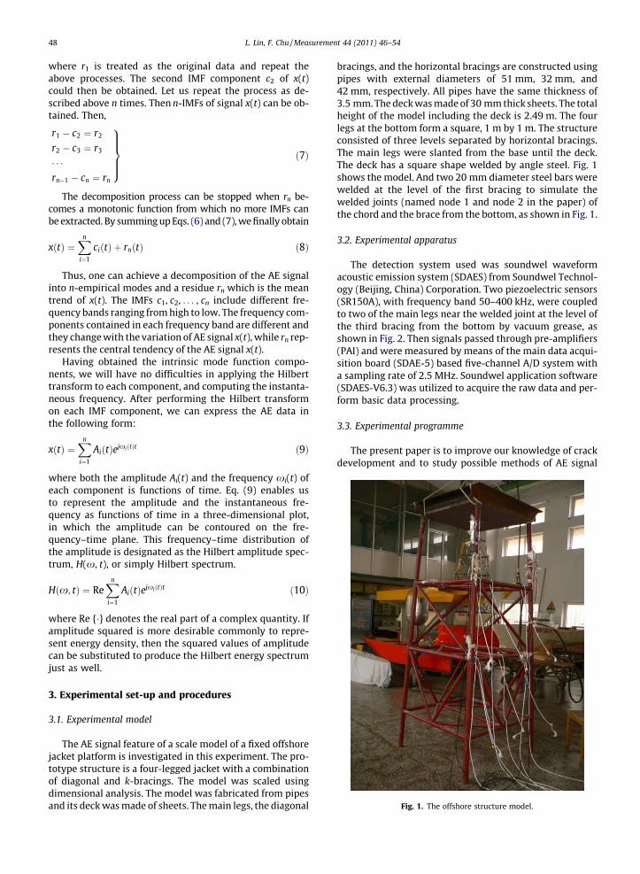
Fig. 1. The offshore structure model.

48 L. Lin, F. Chu / Measurement 44 (2011) 46–54

where r1 is treated as the original data and repeat theabove processes. The second IMF component c2 of x(t)could then be obtained. Let us repeat the process as de-scribed above n times. Then n-IMFs of signal x(t) can be ob-tained. Then,

r1 � c2 ¼ r2

r2 � c3 ¼ r3

� � �rn�1 � cn ¼ rn

9>>>=>>>;

ð7Þ

The decomposition process can be stopped when rn be-comes a monotonic function from which no more IMFs canbe extracted. By summing up Eqs. (6) and (7), we finally obtain

xðtÞ ¼Xn

i¼1

ciðtÞ þ rnðtÞ ð8Þ

Thus, one can achieve a decomposition of the AE signalinto n-empirical modes and a residue rn which is the meantrend of x(t). The IMFs c1, c2, . . . , cn include different fre-quency bands ranging from high to low. The frequency com-ponents contained in each frequency band are different andthey change with the variation of AE signal x(t), while rn rep-resents the central tendency of the AE signal x(t).

Having obtained the intrinsic mode function compo-nents, we will have no difficulties in applying the Hilberttransform to each component, and computing the instanta-neous frequency. After performing the Hilbert transformon each IMF component, we can express the AE data inthe following form:

xðtÞ ¼Xn

i¼1

AiðtÞejxiðtÞt ð9Þ

where both the amplitude Ai(t) and the frequency xi(t) ofeach component is functions of time. Eq. (9) enables usto represent the amplitude and the instantaneous fre-quency as functions of time in a three-dimensional plot,in which the amplitude can be contoured on the fre-quency–time plane. This frequency–time distribution ofthe amplitude is designated as the Hilbert amplitude spec-trum, H(x, t), or simply Hilbert spectrum.

Hðx; tÞ ¼ ReXn

i¼1

AiðtÞejxiðtÞt ð10Þ

where Re {�} denotes the real part of a complex quantity. Ifamplitude squared is more desirable commonly to repre-sent energy density, then the squared values of amplitudecan be substituted to produce the Hilbert energy spectrumjust as well.

3. Experimental set-up and procedures

3.1. Experimental model

The AE signal feature of a scale model of a fixed offshorejacket platform is investigated in this experiment. The pro-totype structure is a four-legged jacket with a combinationof diagonal and k-bracings. The model was scaled usingdimensional analysis. The model was fabricated from pipesand its deck was made of sheets. The main legs, the diagonal

bracings, and the horizontal bracings are constructed usingpipes with external diameters of 51 mm, 32 mm, and42 mm, respectively. All pipes have the same thickness of3.5 mm. The deck was made of 30 mm thick sheets. The totalheight of the model including the deck is 2.49 m. The fourlegs at the bottom form a square, 1 m by 1 m. The structureconsisted of three levels separated by horizontal bracings.The main legs were slanted from the base until the deck.The deck has a square shape welded by angle steel. Fig. 1shows the model. And two 20 mm diameter steel bars werewelded at the level of the first bracing to simulate thewelded joints (named node 1 and node 2 in the paper) ofthe chord and the brace from the bottom, as shown in Fig. 1.

3.2. Experimental apparatus

The detection system used was soundwel waveformacoustic emission system (SDAES) from Soundwel Technol-ogy (Beijing, China) Corporation. Two piezoelectric sensors(SR150A), with frequency band 50–400 kHz, were coupledto two of the main legs near the welded joint at the level ofthe third bracing from the bottom by vacuum grease, asshown in Fig. 2. Then signals passed through pre-amplifiers(PAI) and were measured by means of the main data acqui-sition board (SDAE-5) based five-channel A/D system witha sampling rate of 2.5 MHz. Soundwel application software(SDAES-V6.3) was utilized to acquire the raw data and per-form basic data processing.

3.3. Experimental programme

The present paper is to improve our knowledge of crackdevelopment and to study possible methods of AE signal

Fig. 2. The experimental set-up of offshore structure model underwater.

Fig. 3. AE source simulation test of breaking a lead from the offshorestructure model underwater.

Fig. 4. Knocking test from the offshore structure model underwater.

Fig. 5. Node 2 crack test.

Am

plitu

de

Threshold

Energy

Fig. 6. Feature extraction from an AE hit signal.

0 0.2 0.4 0.6 0.8 1 1.2 1.4 1.6 1.8-1

-0.8

-0.6

-0.4

-0.2

0

0.2

0.4

0.6

0.8

1

time (ms)

Ampl

itude

(v)

Fig. 7. Simulation AE signal wave of breaking a lead.

L. Lin, F. Chu / Measurement 44 (2011) 46–54 49

detection and characterization by using the Hilbert–Huangtransform. The following programme for underwater testswith artificial wave to simulate the offshore conditionswas therefore carried out:

� Recording of simulation AE signals such as pencil leadfractures and knocking the leg as shown in Figs. 3 and 4.� Monitoring of the whole crack growth from starting to

fracturing of T weld joint named node 1 and node 2 dur-ing dragging the steel bar by a cleek as it can be seenfrom Figs. 2 and 5.

4. Analysis

After AE signals are obtained, it is impossible to identifyif numerous data are not analyzed to obtain representative

0 0.2 0.4 0.6 0.8 1 1.2 1.4 1.6 1.8-2

-1.5

-1

-0.5

0

0.5

1

1.5

time (ms)

Ampl

itude

(v)

Fig. 8. Knocking signal wave.

50 L. Lin, F. Chu / Measurement 44 (2011) 46–54

feature value. Therefore, acquisition of feature values is thekey step for higher recognition rate. According to the liter-atures of previous AE research works on offshore struc-

Fig. 9. AE from breaking a pencil lead: (a) en

tures [1–3,5,8–20], feature values which are taken as theidentification data are traditional AE parameters such asamplitude, energy, and hits. A typical acoustic emissionsignal as shown in Fig. 6 is a complex, damped, sinusoidalvoltage vs time plot. These feature values are representedin a statistical way. Amplitude is the maximum value ofthe AE signal that passes through the threshold. Energy isthe power energy of AE waveform that passes throughthreshold and within duration period.

Fig. 7 shows the typical waveform of a pencil lead breakAE signal released during the test as shown in Fig. 3. Fig. 8gives the typical waveform of an AE signal from knockingthe leg test of the offshore structures as shown in Fig. 4.Fig. 9 shows the AE parameter feature value analysis of apencil lead break AE signal. Fig. 10 shows the AE parameterfeature value analysis of an AE signal from knocking the legtest. The energy vs time is shown in Figs. 9a and 10a. Thehit count vs amplitude is shown in Figs. 9b and 10b. Thespikes in the two figures (Figs. 9 and 10) all indicate a jumpof energy, amplitude and hit count when the AE signals arereleased. However, the two figures (Figs. 9 and 10) are sim-ilar. It is shown that the AE parameter method to extract

ergy vs time and (b) hits vs amplitude.

Fig. 10. AE from knocking: (a) energy vs time and (b) hits vs amplitude.

time (ms)

frequ

ency

(kH

z)

0 0.2 0.4 0.6 0.8 1 1.2 1.4 1.6

200

400

600

800

1000

1200

-220-200-180-160-140-120-100-80-60-40-20

Fig. 11. The Hilbert spectrum for the simulation AE signal of breaking alead.

time (ms)

frequ

ency

(kH

z)

0 0.2 0.4 0.6 0.8 1 1.2 1.4 1.6

200

400

600

800

1000

1200

-200

-150

-100

-50

0

Fig. 12. The Hilbert spectrum for the knocking signal wave.

L. Lin, F. Chu / Measurement 44 (2011) 46–54 51

the energy, amplitude and hits as feature values fails toidentify the patterns effectively between a pencil leadbreaking AE signal and a knocking AE signal.

When these data are subject to the HHT method, theHilbert spectrum of the pencil lead break AE signal is givenin Fig. 11 and the knocking AE signal in Fig. 12. These fig-ures give the Hilbert spectrum from which the arrival time

0 1 2 3 4 5 6-1.5

-1

-0.5

0

0.5

1

1.5

time (ms)

Am

plitu

de (v

)

Fig. 13. The AE signal wave of offshore platform model underwater.

52 L. Lin, F. Chu / Measurement 44 (2011) 46–54

and the frequency change of the waves are clearly shownin this energy–frequency–time distribution, the vertical

Fig. 14. The AE signal of offshore platform model underw

coordinate is the frequency (kHz), the horizontal coordi-nates is the time (ms), the energy has the colour map for-mat on the frequency–time plane. Fig. 11 shows that thepencil lead break signal has a frequency range of 0–400 kHz and most of the energy is concentrated in the fre-quency range between 60 kHz and 280 kHz. The highestenergy resides along horizontal belts around 260 kHz,while the lowest persistent energy resides below 60 kHz.Fig. 12 gives that the frequency range of the knocking AEsignal is also 0–400 kHz but most of the energy is concen-trated in the frequency range below 60 kHz. The highestenergy resides along horizontal belts around 60 kHz, whilethe lowest persistent energy resides below 20 kHz. Fromthe two figures, the difference of the frequency rangewhere most of the energy is concentrated can be found.The analysis results show that the HHT method to extractthe energy and frequency as feature values can identifythe patterns effectively between a pencil lead break AE sig-nal and a knocking AE signal.

The AE signal data for the crack of the offshore struc-tures in water were collected by the AE sensors

ater: (a) energy vs time and (b) hits vs amplitude.

Fig. 15. The first five components, C1–C5, for the AE signal of offshore platform model underwater.

time (ms)

frequ

ency

(kH

z)

0 1 2 3 4 5

200

400

600

800

1000

1200

-220-200-180-160-140-120-100-80-60-40-20

Fig. 16. The Hilbert spectrum for the AE signal of offshore platform modelunderwater.

time (ms)

frequ

ency

(kH

z)

0 1 2 3 4 5

200

400

600

800

1000

1200

-200

-150

-100

-50

0

Fig. 17. The Hilbert spectrum for the AE signal C1 of offshore platformmodel underwater.

0 0.2 0.4 0.6 0.8 1 1.2 1.4 1.6 1.8-1

-0.5

0

0.5

1

1.5

time (ms)

Am

plitu

de (v

)

Fig. 18. The crack AE signal wave.

time (ms)

frequ

ency

(kH

z)

0 0.2 0.4 0.6 0.8 1 1.2 1.4 1.6

200

400

600

800

1000

1200

-220-200-180-160-140-120-100-80-60-40-20

Fig. 19. The Hilbert spectrum for the crack AE signal.

L. Lin, F. Chu / Measurement 44 (2011) 46–54 53

54 L. Lin, F. Chu / Measurement 44 (2011) 46–54

(SR150A). Fig. 13 shows the raw data of the whole crackgrowth from starting to fracturing of T weld joint namednode 2 during dragging the steel bar by a cleek as it canbe seen from Fig. 5. Of course these are not real offshorecondition and the real offshore crack AE signals, but theyallow to observe the whole crack development, to improveour knowledge of AE generation mechanisms, and to studypossible methods of signal detection and characterization.In the past, amplitude, energy, hits or other parameterswere used to classify and recognize the evolution quantita-tively [1–3,5,8,18]. Fig. 14 shows the AE parameter featurevalue analysis of the AE signal. Sudden increase of energy,amplitude and hits can be seen. The HHT method yields 17IMF components from the data and the first five IMF com-ponents, C1–C5, are shown in Fig. 15. The Hilbert spectrumis given in Fig. 16. From the Hilbert spectrum, we can seebefore 1.6 ms the highest energy resides along horizontalbelts around 260 kHz with a frequency range of 0–400 kHz and most of the energy is concentrated in the fre-quency range between 60 kHz and 280 kHz, while after1.6 ms most of the energy is concentrated in the frequencyrange around 60 kHz and the diffused energy resides above60 kHz. Fig. 17 shows the Hilbert spectrum of the first IMFcomponent which is the major energy concentration com-ponent. One frequency band centers around 260 kHz be-fore 1.6 ms which is the crack signal feature similar tothe AE signal feature of breaking a lead, 60 kHz after1.6 ms which is the knocking of the leg signal feature afterthe tensile failure steel bar of the cleek and there appearsenergy increase from 0.81 ms. Fig. 18 shows the crack AEsignal waveform before 1.6 ms and Fig. 19 shows the Hil-bert spectrum of the waveform before 1.6 ms. The featuresof frequency and energy from the occurrence to end of thecrack are vividly portrayed by the Hilbert spectrum beforeit is visible. The energy in the feature frequency band be-tween 60 kHz and 280 kHz shows a sudden increase from0.81 ms because of the rapid growth of crack. But only afew features are suggested by using AE parameter analysismethod which confuse the crack and the knocking AE sig-nal as shown in Fig. 14.

5. Conclusions

The experiments here are bringing positive elements tothe HHT method to the applicability of AE techniques tothe offshore structures. The Hilbert–Huang transform pro-vides an effective way for interpreting the nonlinear/non-stationary AE signals in the offshore structure model bydecomposing the signal into different IMF components toobtain the Hilbert spectrum. Energy carried by each IMFcomponent of the AE signal was analyzed by consideringthe full waveform instead of only AE amplitude, energyor hit count. The comparison between the existing AE tech-nique and the HHT–AE method shows that the HHT–AEmethod has an advantage over the conventional AE meth-od in processing the AE data of the offshore structure mod-el attributing to the HHT adaptive feature characterization.

Therefore, this will be helpful for improving the signalcharacterization techniques in order to avoid any wrongconclusions as to the existence of a crack in comparisonwith the AE parameter method for the crack monitoringin offshore structures.

References

[1] M. Silk, N. Williams, K. Bainton, Potential role of NDT techniques inthe monitoring of fixed offshore structures, British Journal of Non-Destructive Testing 17 (3) (1975) 83–87.

[2] L.M. Rogers, Crack detection using acoustic emission methods –fundamentals and applications, Key Engineering Materials 293–294(2005) 33–46.

[3] P. Dumousseau, P. Laffont, J. Thebault, Experimental study ofacoustic emission monitoring of crack propagation in offshore steeltubular joint, in: Proceedings of the Annual Offshore TechnologyConference, vol. 1, 1979, pp. 593–599.

[4] L. Rogers, J.P. Hansen, C. Webborn, Application of acoustic emissionanalysis to the integrity monitoring of offshore steel productionplatforms, Materials Evaluation 38 (8) (1980) 39–49.

[5] Z. Wang, J. Li, W. Ke, et al., Characteristics of acoustic emission forA537 structural steel during fatigue crack propagation, ScriptaMetallurgica et Materialia 27 (5) (1992) 641–646.

[6] N. Huang, Z. Shen, S. Long, et al., The empirical mode decompositionand the Hilbert spectrum for nonlinear and non-stationary timeseries analysis, Proceedings of the Royal Society of London Series A –Mathematical Physical and Engineering Sciences 454 (1971) (1998)903–995.

[7] H. Li, Y.P. Zhang, H.Q. Zheng, Hilbert–Huang transform and marginalspectrum for detection and diagnosis of localized defects in rollerbearings, Journal of Mechanical Science and Technology 23 (2)(2009) 291–301.

[8] V. Peters, Offshore platform NDT instrumentation requirements, in:Conference on the Operation of Instruments in AdverseEnvironments 1976, 1977, pp. 13–18.

[9] W. Harris, Report of a preliminary survey of NDT technology withspecial reference to offshore structures, British Journal of Non-Destructive Testing 25 (3) (1983) 117–120.

[10] V. Bindal, Testing of underwater offshore structures, Chemical Age ofIndia 35 (10) (1984) 721–725.

[11] A. Nielsen, Factors to consider before deciding on an AE examinationof a steel structure, European Journal of Non-Destructive Testing 2(4) (1993) 127–134.

[12] L. Rogers, Sizing fatigue cracks in offshore structures by the acousticemission method, Insight: Non-Destructive Testing and ConditionMonitoring 36 (9) (1994) 661.

[13] M. Rampolli, Structural maintenance of Agip platforms, Insight:Non-Destructive Testing and Condition Monitoring 39 (6) (1997)405–407.

[14] L. Rogers, Crack detection by acoustic emission, Journal of OffshoreTechnology 6 (2) (1998) 35–36.

[15] L. Rogers, Use of acoustic emission methods for crack growthdetection in offshore and other structures, International MaritimeTechnology 110 (Pt. 3) (1998) 171–180.

[16] C. Greene, M. Mclennan, R. Norman, et al., Directional frequency andrecording (DIFAR) sensors in seafloor recorders to locate callingbowhead whales during their fall migration, Journal of theAcoustical Society of America 116 (2) (2004) 799–813.

[17] K. Burnham, S. Pierce, Acoustic techniques for wind turbine blademonitoring, Key Engineering Materials 347 (2007) 639–644.

[18] L. Rogers, J. Hansen, T. Webborn, Application of acoustic emissionanalysis to the integrity monitoring of offshore steel productionplatforms, Materials Evaluation 38 (8) (1980) 39–49.

[19] C. Thaulow, T. Berge, Acoustic emission monitoring of corrosionfatigue crack growth in offshore steel, NDT&E International 17 (3)(1984) 147–153.

[20] Li Lin, De-You Zhao, Identification of acoustic emission signals ofoffshore structures with both local wave method and neuralnetwork, Harbin Gongcheng Daxue Xuebao/Journal of HarbinEngineering University 29 (7) (2008) 663–667.