
Feature extraction 1.Introduction 2.T-test 3.Signal Noise Ratio (SNR) 4.Linear Correlation...
62
Feature extraction 1.Introduction 2.T-test 3.Signal Noise Ratio (SNR) 4.Linear Correlation Coefficient (LCC) 5.Principle component analysis (PCA) 6.Linear discriminant analysis (LDA)
-
Upload
benjamin-wilkerson -
Category
Documents
-
view
227 -
download
2
Transcript of Feature extraction 1.Introduction 2.T-test 3.Signal Noise Ratio (SNR) 4.Linear Correlation...
Feature extraction1. Introduction2. T-test3. Signal Noise Ratio (SNR)4. Linear Correlation Coefficient (LCC)5. Principle component analysis (PCA)6. Linear discriminant analysis (LDA)

Feature reduction vs feature selection
• Feature reduction– All original features are used– The transformed features are linear combinations
of the original features.
• Feature selection– Only a subset of the original features are used.

Why feature reduction?
• Most machine learning and data mining techniques may not be effective for high-dimensional data – Curse of Dimensionality– Query accuracy and efficiency degrade rapidly as the
dimension increases.
• The intrinsic dimension may be small. – For example, the number of genes responsible for a
certain type of disease may be small.
Why feature reduction?
• Visualization: projection of high-dimensional data onto 2D or 3D.
• Data compression: efficient storage and retrieval.
• Noise removal: positive effect on query accuracy.

Applications of feature reduction
• Face recognition• Handwritten digit recognition• Text mining• Image retrieval• Microarray data analysis• Protein classification
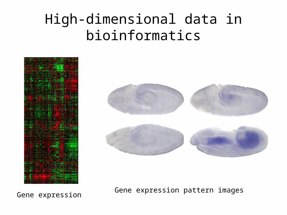
High-dimensional data in bioinformatics
Gene expressionGene expression pattern images
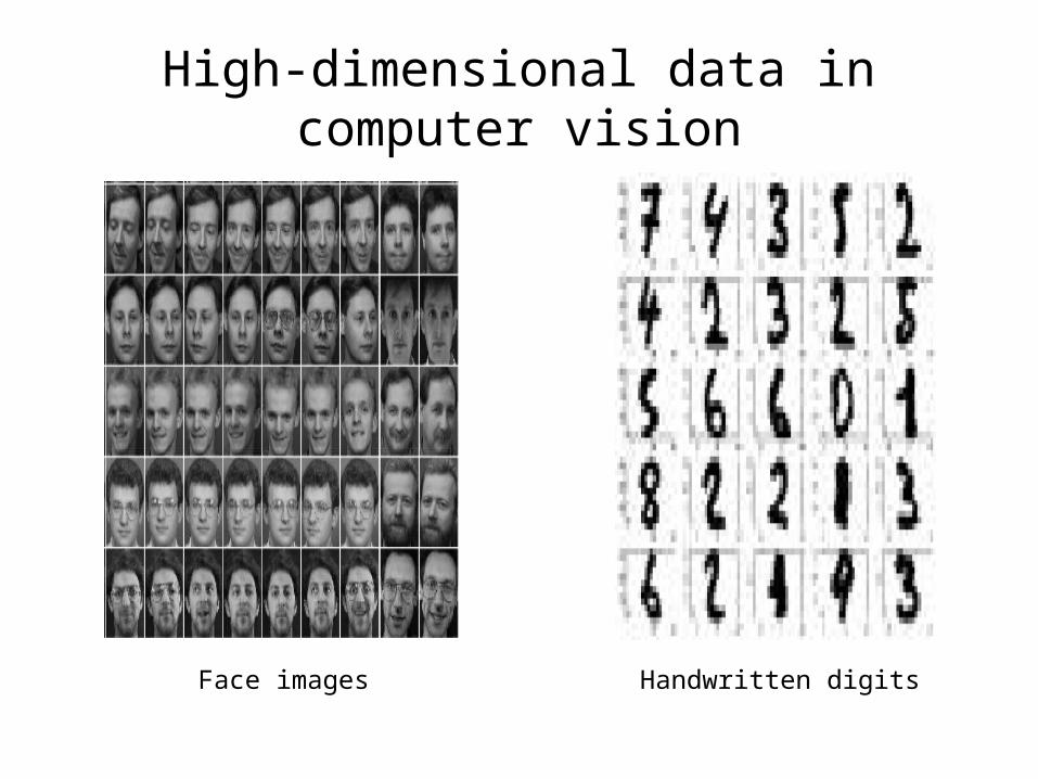
High-dimensional data in computer vision
Face images Handwritten digits
Principle component analysis (PCA)
Motivation Example:
• Given 53 blood and urine samples (features) from 65 people.
• How can we visualize the measurements?

PCA
• Matrix format (65x53)H - W B C H - R B C H - H g b H - H c t H - M C V H - M C H H - M C H CH - M C H C
A 1 8 . 0 0 0 0 4 . 8 2 0 0 1 4 . 1 0 0 0 4 1 . 0 0 0 0 8 5 . 0 0 0 0 2 9 . 0 0 0 0 3 4 . 0 0 0 0
A 2 7 . 3 0 0 0 5 . 0 2 0 0 1 4 . 7 0 0 0 4 3 . 0 0 0 0 8 6 . 0 0 0 0 2 9 . 0 0 0 0 3 4 . 0 0 0 0
A 3 4 . 3 0 0 0 4 . 4 8 0 0 1 4 . 1 0 0 0 4 1 . 0 0 0 0 9 1 . 0 0 0 0 3 2 . 0 0 0 0 3 5 . 0 0 0 0
A 4 7 . 5 0 0 0 4 . 4 7 0 0 1 4 . 9 0 0 0 4 5 . 0 0 0 0 1 0 1 . 0 0 0 0 3 3 . 0 0 0 0 3 3 . 0 0 0 0
A 5 7 . 3 0 0 0 5 . 5 2 0 0 1 5 . 4 0 0 0 4 6 . 0 0 0 0 8 4 . 0 0 0 0 2 8 . 0 0 0 0 3 3 . 0 0 0 0
A 6 6 . 9 0 0 0 4 . 8 6 0 0 1 6 . 0 0 0 0 4 7 . 0 0 0 0 9 7 . 0 0 0 0 3 3 . 0 0 0 0 3 4 . 0 0 0 0
A 7 7 . 8 0 0 0 4 . 6 8 0 0 1 4 . 7 0 0 0 4 3 . 0 0 0 0 9 2 . 0 0 0 0 3 1 . 0 0 0 0 3 4 . 0 0 0 0
A 8 8 . 6 0 0 0 4 . 8 2 0 0 1 5 . 8 0 0 0 4 2 . 0 0 0 0 8 8 . 0 0 0 0 3 3 . 0 0 0 0 3 7 . 0 0 0 0
A 9 5 . 1 0 0 0 4 . 7 1 0 0 1 4 . 0 0 0 0 4 3 . 0 0 0 0 9 2 . 0 0 0 0 3 0 . 0 0 0 0 3 2 . 0 0 0 0 Inst
ance
s
Features
Difficult to see the correlations between the features...
PCA - Data Visualization
0 10 20 30 40 50 60 700
0.20.40.60.811.21.41.61.8
Person
H-B
an
ds
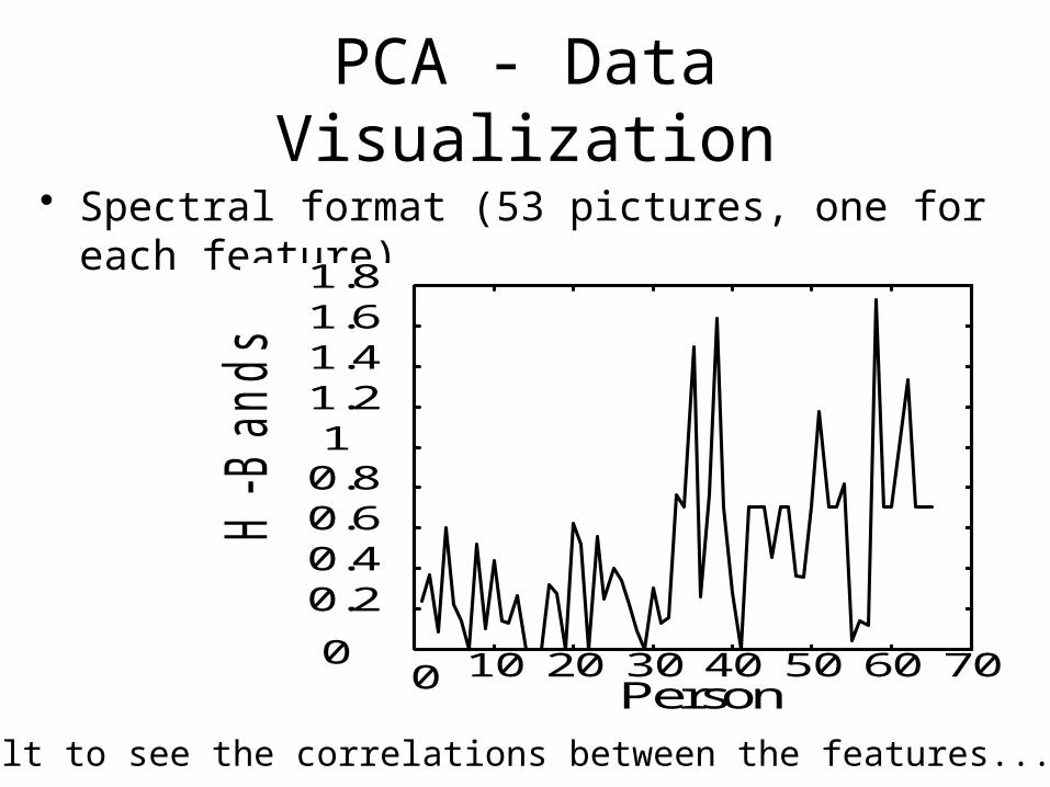
• Spectral format (53 pictures, one for each feature)
Difficult to see the correlations between the features...

0 50 150 250 350 45050100150200250300350400450500550
C-Triglycerides
C-L
DH
0100
200300
400500
0200
4006000
1
2
3
4
C-TriglyceridesC-LDH
M-E
PI
Bi-variate Tri-variate
PCA - Data Visualization
How can we visualize the other variables???… difficult to see in 4 or higher dimensional spaces...

Data Visualization
• Is there a representation better than the coordinate axes?
• Is it really necessary to show all the 53 dimensions?– … what if there are strong correlations between the features?
• How could we find the smallest subspace of the 53-D space that keeps the most information about the original data?
• A solution: Principal Component Analysis
Principle Component Analysis
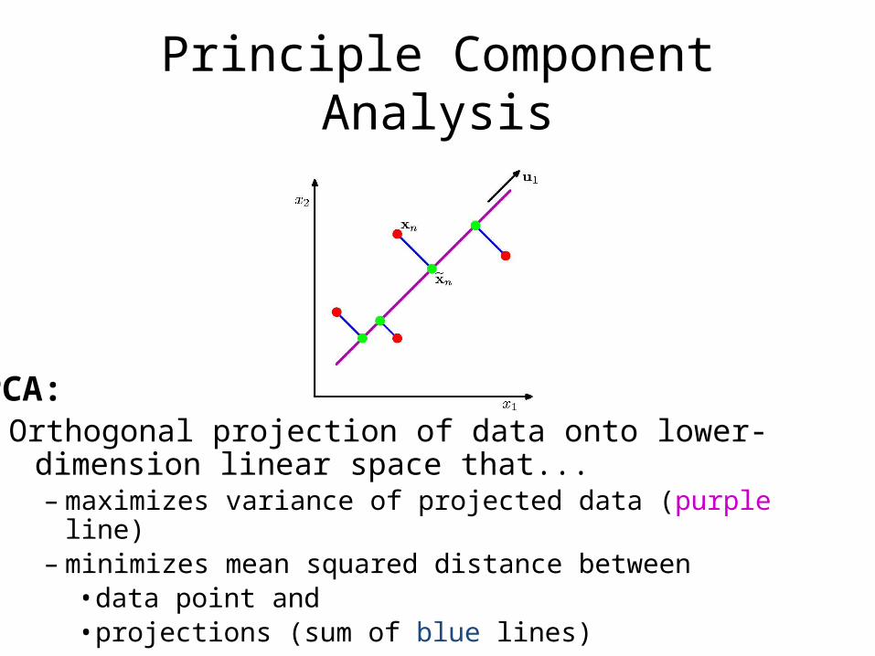
Orthogonal projection of data onto lower-dimension linear space that...– maximizes variance of projected data (purple line)– minimizes mean squared distance between
• data point and • projections (sum of blue lines)
PCA:

Principle Components AnalysisIdea:
– Given data points in a d-dimensional space, project into lower dimensional space while preserving as much information as possible
• Eg, find best planar approximation to 3D data• Eg, find best 12-D approximation to 104-D data
– In particular, choose projection that minimizes squared error in reconstructing original data

• Vectors originating from the center of mass• Principal component #1 points
in the direction of the largest variance.• Each subsequent principal component…
– is orthogonal to the previous ones, and – points in the directions of the largest variance of
the residual subspace
The Principal Components

2D Gaussian dataset

1st PCA axis
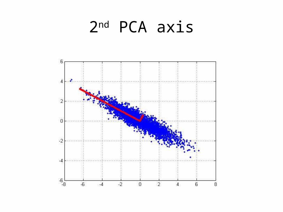
2nd PCA axis

PCA algorithm I (sequential)
m
i
k
ji
Tjji
Tk m 1
21
11
})]({[1
maxarg xwwxwww
}){(1
maxarg1
2i
11
m
i
T
mxww
w
We maximize the variance of the projection in the residual subspace
We maximize the variance of projection of x
x’ PCA reconstruction
Given the centered data {x1, …, xm}, compute the principal vectors:
1st PCA vector
kth PCA vector
w1(w1Tx)
w2(w2Tx)
x
w1
w2
x’=w1(w1Tx)+w2(w2
Tx)
w

PCA algorithm II (sample covariance matrix)
• Given data {x1, …, xm}, compute covariance matrix
• PCA basis vectors = the eigenvectors of
• Larger eigenvalue more important eigenvectors
m
i
Tim 1
))((1
xxxx
m
iim 1
1xxwhere
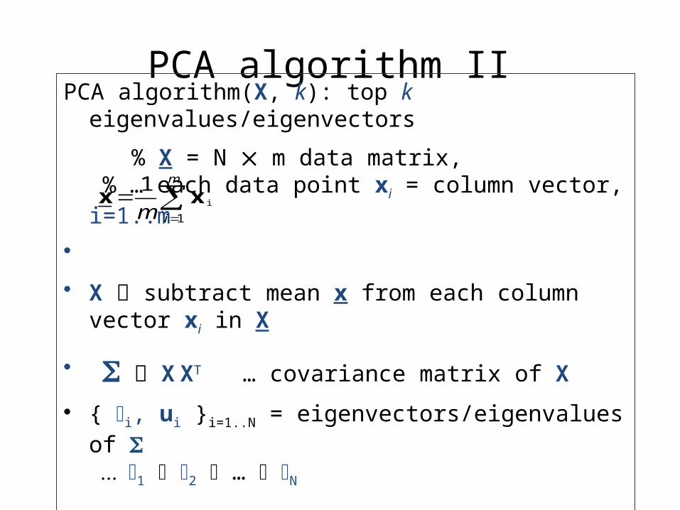
PCA algorithm II PCA algorithm(X, k): top k eigenvalues/eigenvectors
% X = N m data matrix, % … each data point xi = column vector, i=1..m
•
• X subtract mean x from each column vector xi in X
• X XT … covariance matrix of X
• { i, ui }i=1..N = eigenvectors/eigenvalues of ... 1 2 … N
• Return { i, ui }i=1..k
% top k principle components
m
im 1
1ixx

PCA algorithm III (SVD of the data matrix)
Singular Value Decomposition of the centered data matrix X.
Xfeatures samples = USVT
X VTSU=
samples
significant
noise
nois
e noise
sign
ific
ant
sig.
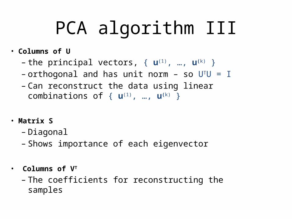
PCA algorithm III• Columns of U
– the principal vectors, { u(1), …, u(k) }– orthogonal and has unit norm – so UTU = I– Can reconstruct the data using linear combinations of
{ u(1), …, u(k) }
• Matrix S
– Diagonal– Shows importance of each eigenvector
• Columns of VT
– The coefficients for reconstructing the samples
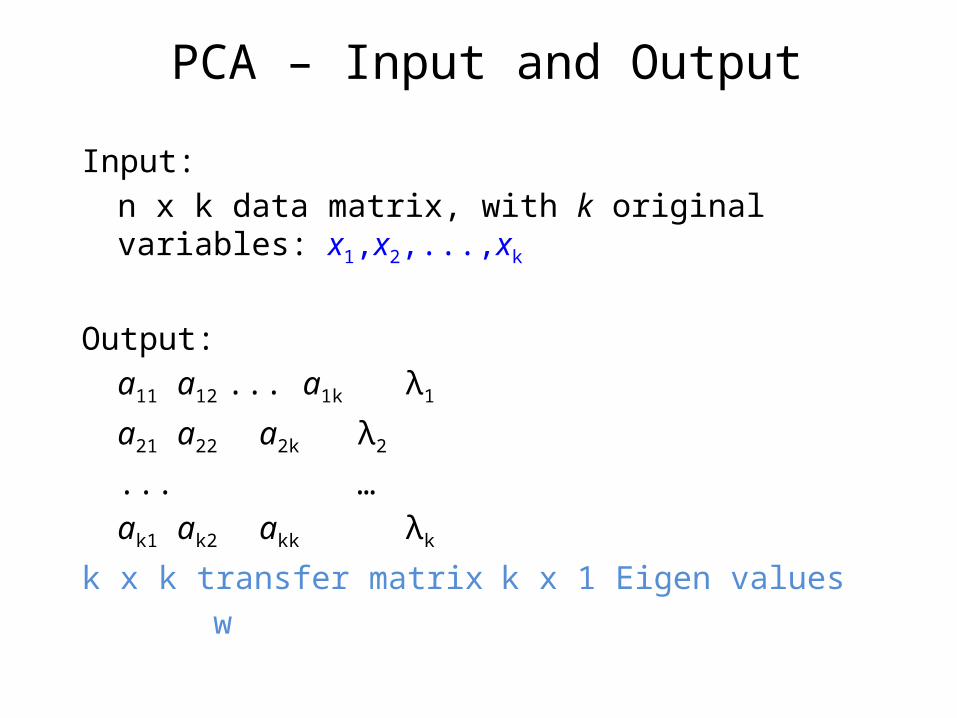
Input:n x k data matrix, with k original variables: x1,x2,...,xk
Output:a11 a12 ... a1k λ1
a21 a22 a2k λ2
... …ak1 ak2 akk λk
k x k transfer matrix k x 1 Eigen values w
PCA – Input and Output

From k original variables: x1,x2,...,xk:
Produce k new variables: y1,y2,...,yk:
y1 = a11x1 + a12x2 + ... + a1kxk
y2 = a21x1 + a22x2 + ... + a2kxk
...yk = ak1x1 + ak2x2 + ... + akkxk
such that:
yi's are uncorrelated (orthogonal)y1 explains as much as possible of original variance in data sety2 explains as much as possible of remaining varianceetc.
yi's arePrincipal Components
PCA – usage (k to k transfer)

PCA - usage
n x kdata
k x kwT
n x ktransferred
datax =
n x kdata
k x tW’T
n x ttransfe
rreddata
x = Dimensionreduction
Direct transfer
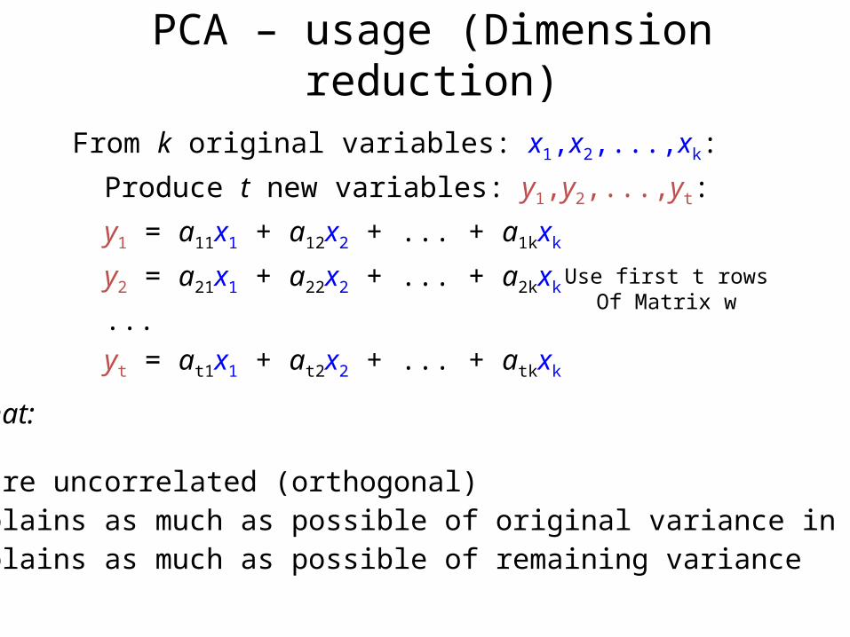
From k original variables: x1,x2,...,xk:
Produce t new variables: y1,y2,...,yt:
y1 = a11x1 + a12x2 + ... + a1kxk
y2 = a21x1 + a22x2 + ... + a2kxk
...yt = at1x1 + at2x2 + ... + atkxk
such that:
yi's are uncorrelated (orthogonal)y1 explains as much as possible of original variance in data sety2 explains as much as possible of remaining varianceetc.
PCA – usage (Dimension reduction)
Use first t rowsOf Matrix w
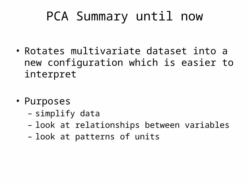
PCA Summary until now
• Rotates multivariate dataset into a new configuration which is easier to interpret
• Purposes– simplify data– look at relationships between variables– look at patterns of units

Example of PCA on Iris Data

PCA application on image compression

Original Image
• Divide the original 372x492 image into patches:• Each patch is an instance that contains 12x12 pixels on a grid
• View each as a 144-D vector

L2 error and PCA dim
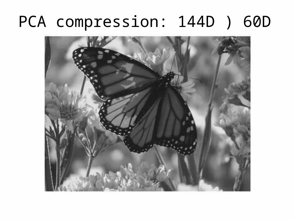
PCA compression: 144D ) 60D
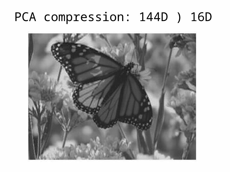
PCA compression: 144D ) 16D
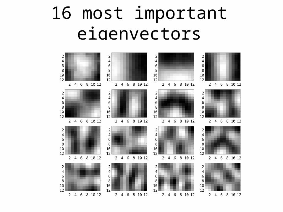
16 most important eigenvectors
2 4 6 8 10 12
2468
1012
2 4 6 8 10 12
2468
1012
2 4 6 8 10 12
2468
1012
2 4 6 8 10 12
2468
1012
2 4 6 8 10 12
2468
1012
2 4 6 8 10 12
2468
1012
2 4 6 8 10 12
2468
1012
2 4 6 8 10 12
2468
1012
2 4 6 8 10 12
2468
1012
2 4 6 8 10 12
2468
1012
2 4 6 8 10 12
2468
1012
2 4 6 8 10 12
2468
1012
2 4 6 8 10 12
2468
1012
2 4 6 8 10 12
2468
1012
2 4 6 8 10 12
2468
1012
2 4 6 8 10 12
2468
1012

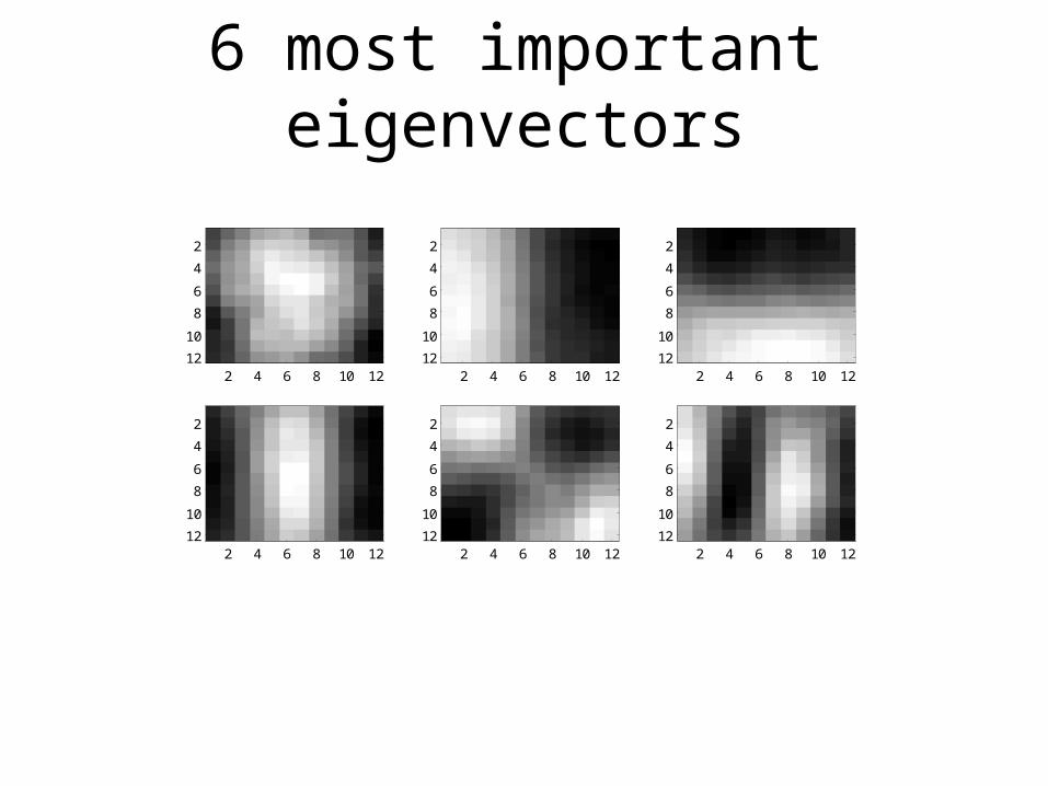
PCA compression: 144D ) 6D
2 4 6 8 10 12
2
4
6
8
10
122 4 6 8 10 12
2
4
6
8
10
122 4 6 8 10 12
2
4
6
8
10
12
2 4 6 8 10 12
2
4
6
8
10
122 4 6 8 10 12
2
4
6
8
10
122 4 6 8 10 12
2
4
6
8
10
12
6 most important eigenvectors

PCA compression: 144D ) 3D

2 4 6 8 10 12
2
4
6
8
10
12
2 4 6 8 10 12
2
4
6
8
10
12
2 4 6 8 10 12
2
4
6
8
10
12
3 most important eigenvectors

PCA compression: 144D ) 1D
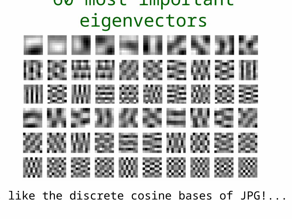
60 most important eigenvectors
Looks like the discrete cosine bases of JPG!...

2D Discrete Cosine Basis
http://en.wikipedia.org/wiki/Discrete_cosine_transform

PCA for image compression
p=1 p=2 p=4 p=8
p=16 p=32 p=64 p=100Original Image

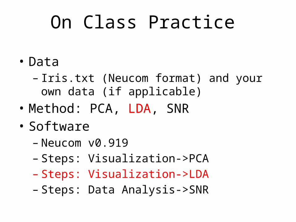
On Class Practice
• Data – Iris.txt (Neucom format) and your own data (if
applicable)• Method: PCA, LDA, SNR• Software
– Neucom v0.919– Steps: Visualization->PCA– Steps: Visualization->LDA– Steps: Data Analysis->SNR
Linear Discriminant Analysis• First applied by M. Barnard at the suggestion
of R. A. Fisher (1936), Fisher linear discriminant analysis (FLDA):
• Dimension reduction
– Finds linear combinations of the features X=X1,...,Xd with large ratios of between-groups to within-groups sums of squares - discriminant variables;
• Classification
– Predicts the class of an observation X by the class whose mean vector is closest to X in terms of the discriminant variables
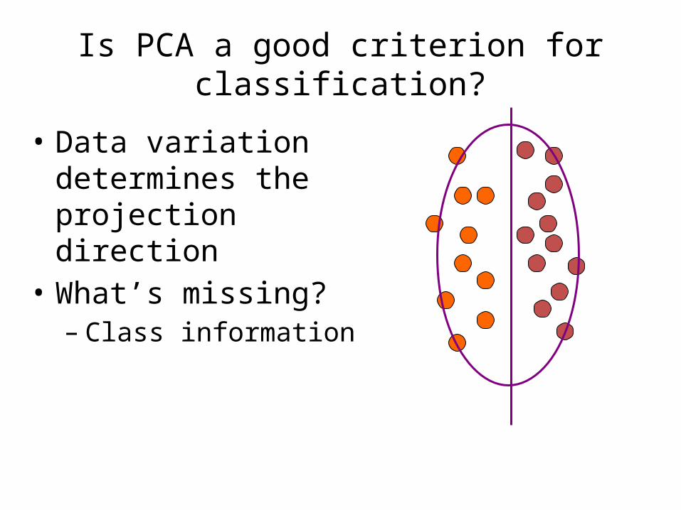
Is PCA a good criterion for classification?
• Data variation determines the projection direction
• What’s missing?– Class information
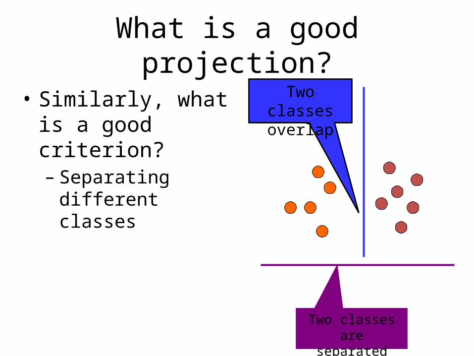
What is a good projection?
• Similarly, what is a good criterion? – Separating different
classes
Two classes overlap
Two classes are separated

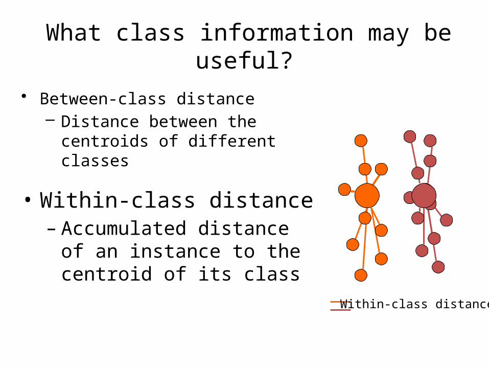
What class information may be useful?
Between-class distance
• Between-class distance– Distance between the centroids
of different classes
What class information may be useful?
Within-class distance
• Within-class distance– Accumulated distance of an
instance to the centroid of its class
• Between-class distance– Distance between the centroids of
different classes

Linear discriminant analysis
• Linear discriminant analysis (LDA) finds most discriminant projection by maximizing between-class distance and minimizing within-class distance

Linear discriminant analysis
• Linear discriminant analysis (LDA) finds most discriminant projection by maximizing between-class distance and minimizing within-class distance

Notations
nm
A
1A
A
2A kA
Data matrix
Training data from different from 1, 2, …, k

Notations
• Between-class scatterTbbb HHS
• Properties:• Between-class distance = trace of between-class scatter (I.e., the
summation of diagonal elements of the scatter)• Within-class distance = trace of within-class scatter
cc 1
bH
cc 2 cck
nm
classes all of centroid theis
classith of centroid theis
c
ci
• Within-class scatter
Twww HHS
nm
A
11 cA
wH
22 cA kk cA

Discriminant criterion
• Discriminant criterion in mathematical formulation
– Between-class scatter matrix
– Within-class scatter matrix
• The optimal transformation is given by solving a generalized eigenvalue problem
wSbS
)(trace
)(tracemaxarg
GSG
GSG
wT
bT
G
bw SS 1

Graphical view of classification
d
n
dnA
n
K-1
)1( knLAK-1
d
)1( kdG
1K-1
)1(1 kLh
Find the nearest neighborOr nearest centroid
d1
dh 1
A test data point h

1. For each class Ci 1 , caluculate mean iu , covariance matrix iand a
priori class probability iP
N
NP i
i , with iN number of vectors in class i
2. Calculate scatter matrices wS and BS :
C
iiiw PS
1
C
i
TiiiB uuuuPS
1
))(( , where
C
iiiuPu
1
3. Do eigenanalysis of Tw VDVS (Matlab eig)
4. Discard any zero eigenvalues of wS with their eigenvectors
5. Form whitening transform 2/1VDB 6. Obtain new BSBS B
TB
7. Do eigenanalysis of TB UUS (Matlab eig)
8. Select the M biggest eigenvalues M 1 9. Pack their associated eigenvectors into the transformation matrix
][ 1 MuuBW
10. Transform the data via TxWy
LDA Computation

Input:n x k data matrix, with k original variables: x1,x2,...,xk
Output:a11 a12 ... a1k λ1
a21 a22 a2k λ2
... …ak1 ak2 akk λk
k x k transfer matrix k x 1 Eigen values w
LDA – Input and Output

LDA - usage
n x kdata
k x kwT
n x ktransferred
datax =
n x kdata
k x tW’T
n x ttransfe
rreddata
x = Dimensionreduction
Direct transfer

LDA Principle: Maximizing between class distances and Minimizing within class distances

An Example: Fisher’s Iris Data
Actual Group
Number of Observations
Predicted Group
Setosa Versicolor Virginica
SetosaVersicolorVirginica
505050
5000
0481
0249
Table 1: Linear Discriminant Analysis (APER = 0.0200)

LDA on Iris Data
On Class Practice
• Data – Iris.txt (Neucom format) and your own data (if
applicable)• Method: PCA, LDA, SNR• Software
– Neucom v0.919– Steps: Visualization->PCA– Steps: Visualization->LDA– Steps: Data Analysis->SNR