fealko thesis water resources - University of Idaho · For surface water collection purposes a...

A Probabilistic Water Resources Assessment of the Paradise Creek Watershed

A Thesis

Presented in Partial Fulfillment of the Requirements for the

Degree of Master of Science

with a

Major in Civil Engineering

in the

College of Graduate Studies

University of Idaho

By

Jeffrey J. Fealko

August 2003

Major Professor: Fritz Fiedler, Ph.D., PE

ii

ii

AUTHORIZATION TO SUBMIT

THESIS

This thesis of Jeffrey J. Fealko, submitted for the degree of Master of Science with a major in Civil Engineering and titled “A Probabilistic Water Resources Assessment of the Paradise Creek Watershed,” has been reviewed in final form. Permission, as indicated by the signatures and dates given below, is now granted to submit final copies to the College of Graduate Studies for approval. Major Professor ____________________________________Date___________ Fritz Fiedler Committee Members ____________________________________Date____________ Jim Liou ____________________________________Date____________ Jerry Fairley Department Administrator ____________________________________Date____________ Sunil Sharma Discipline’s College Dean ____________________________________Date____________ David Thompson Final Approval and Acceptance by the College of Graduate Studies ____________________________________Date____________ Margrit von Braun

iii

iii

A Probabilistic Water Resources Assessment of the Paradise Creek Watershed

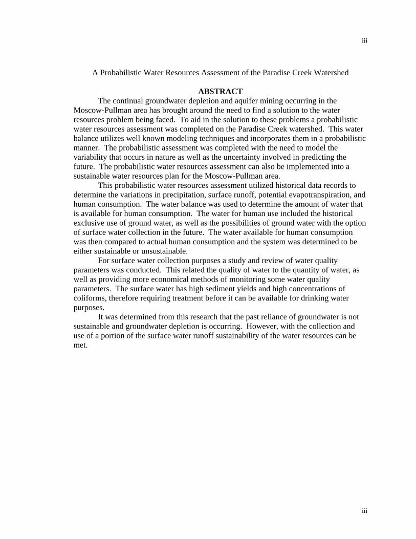
ABSTRACT The continual groundwater depletion and aquifer mining occurring in the Moscow-Pullman area has brought around the need to find a solution to the water resources problem being faced. To aid in the solution to these problems a probabilistic water resources assessment was completed on the Paradise Creek watershed. This water balance utilizes well known modeling techniques and incorporates them in a probabilistic manner. The probabilistic assessment was completed with the need to model the variability that occurs in nature as well as the uncertainty involved in predicting the future. The probabilistic water resources assessment can also be implemented into a sustainable water resources plan for the Moscow-Pullman area. This probabilistic water resources assessment utilized historical data records to determine the variations in precipitation, surface runoff, potential evapotranspiration, and human consumption. The water balance was used to determine the amount of water that is available for human consumption. The water for human use included the historical exclusive use of ground water, as well as the possibilities of ground water with the option of surface water collection in the future. The water available for human consumption was then compared to actual human consumption and the system was determined to be either sustainable or unsustainable. For surface water collection purposes a study and review of water quality parameters was conducted. This related the quality of water to the quantity of water, as well as providing more economical methods of monitoring some water quality parameters. The surface water has high sediment yields and high concentrations of coliforms, therefore requiring treatment before it can be available for drinking water purposes. It was determined from this research that the past reliance of groundwater is not sustainable and groundwater depletion is occurring. However, with the collection and use of a portion of the surface water runoff sustainability of the water resources can be met.

iv

iv

ACKNOWLEDGEMENTS I would first like to acknowledge and thank the Palouse Basin Aquifer Committee for the continued funding and encouragement to complete this research. A thanks also goes out to the Hydroinformatics Laboratory at the University of Idaho for the initial funding of this research. I would also like to acknowledge my major advisor Fritz Fiedler for his patience and continued prodding. Without him this thesis would be nonexistent. I also need to thank Jim Liou and Jerry Fairley for their critical reviews of this thesis. I would like to especially thank my friends and family members who put up with me for the past two years. The encouragement and support received from you is beyond what words can express. I am truly in your debt.

v

v

Table of Contents Authorization to Submit Thesis ……………………………………………….. ii

Abstract ……………………………………………………………………….. iii

Acknowledgements ……………………………………………………………….. v

Table of Contents ……………………………………………………………….. vi

List of Figures ……………………………………………………………………….. viii

List of Tables ……………………………………………………………………….. x

Chapter 1 ……………………………………………………………………….. 1

Introduction ……………………..…………………………….….……….. 1

Objectives …………………………………………………….…………. 7

Purpose ………..……...…………..……………….………….. 7

Scope …….….……………………………………………………… 8

Chapter II ……………………………………………………………………….. 9

Literature Review …………………………..…………………………… 9

Sustainability ……………………….………………………………. 9

Water Balance ……………………………….………………………. 15

Chapter III ……………………………………………………………………….. 27

Methods ……………………………………………………………….. 27

Chapter IV ……………………………………………………………………….. 37

Watershed Description ……………………….………………………. 37

Chapter V ……………………………………………………………………….. 41

Results ……………………………………………………………………….. 41

vi

vi

Precipitation ……………………………………………………….. 41

Surface Runoff ……………………………………………….. 43

Evapotranspiration ……………………………………………….. 45

Groundwater ………………..……………………………………… 48

Soil Moisture ……………………………………………………….. 49

Deep Percolation ……………………………………………….. 49

Water Resources Assessment ……………………………………….. 51

Uncertainty ……………………………………………………….. 57

Chapter VI ……………………………………………………………………….. 63

Water Quality Parameters ……………………………………………….. 63

Results ……………………………………………………………………….. 67

Chapter VII ……………………………………………………………………….. 74

Conclusions ……………………………………………………………….. 74

Recommendations on Sustainability ……………………………….. 77

Future Research ……………………………………………….. 77

Appendix A. Water Quantity ……………………………………………………….. 94

Precipitation ……………………………………………………………….. 95

Surface Runoff ……………………………………………………….. 108

Potential Evapotranspiration ……………………………………………….. 121

Appendix B. Water Quality ……………………………………………………….. 134

IASCD Water Quality ……………………………………………………….. 135

University of Idaho Water Quality ……………………………………….. 155

vii

vii

List of Figures

Figure 1. Regional Map ……………………………………………………….. 4

Figure 2. Levels of uncertainty (Simonovic, 1997) ……….………………………. 14

Figure 3. Water balance and water resources balance (Miloradov, 1995) ……….. 17

Figure 4. a. Current water resources balance ……………………………….. 28

b. New water balance for sustainable water resources management .. 28

Figure 5. Location of gaging stations ……………………………………….. 36

Figure 6. Digital elevation map of Paradise Creek watershed …………….…. 38

Figure 7. Hypsometric curve of Paradise Creek watershed …………………….…. 38

Figure 8. Landuse within Paradise Creek watershed …………………………….…. 40

Figure 9. Distribution of average annual precipitation ……………………….. 42

Figure 10. Probability of exceedence of annual precipitation based on the LPIII

distribution function ……………….………………………………. 43

Figure 11. Exceedence probability of annual discharge …………….…….…… 44

Figure 12. PET probability of exceedence ……………………………………….. 47

Figure 13. Deep percolation probability of exceedence ……..………………… 51

Figure 14. Combined water balance probabilities of exceedence functions .………. 52

Figure 15. Percentage of annual water consumed ……………….………………. 52

Figure 16. Human consumption and trend line ……….………………………. 54

Figure 17. Exceedence probability of variation from consumption trend ….……. 54

Figure 18. Extended precipitation and PET record water balance probabilities of

exceedence ……….………………………………………………. 61

Figure 19. Water pH levels in Paradise Creek ………………….……………. 68

viii

viii

Figure 20. Yearly nitrate levels for Darby and MWWTP stations ……….………. 69

Figure 21. Yearly temperature variations for Darby and MWWTP stations .………. 70

Figure 22. Turbidity and discharge relationship for MWWTP ………….……. 71

Figure 23. Turbidity and total suspended solids relationship for Darby and MWWTP

stations ……………………………….………………………………. 71

Figure 24. Total dissolved solids and electroconductivity in Paradise Creek .. 72

Figure 25. Turbidity and total phosphorus in Paradise Creek ……………….. 73

Figure 26. Water content between bare soil and mulch covered soil (Wade, 2003) .. 84

ix

ix

List of Tables

Table 1. Average precipitation values and historical scale factors …………….…. 32

Table 2. Water quality testing methods/instruments ……………………………….. 36

Table 3. Exceedence probabilities for precipitation over the watershed …...…... 43

Table 4. Exceedence probabilities for discharge from the watershed .………. 45

Table 5. Monthly crop coefficients for PET calculations …………………….…. 46

Table 6. Monthly and annual PET probabilities of exceedence ……….………. 48

Table 7. Annual deep percolation probabilities of exceedence ……….………. 51

Table 8. Past 5 years water resources assessment and PHC-AHC ratio …….…. 56

Table 9. Modified past 5 years water resources assessment and PHC-AHC ratio .. 57

Table 10. Past 5 years PHC-AHC ratio for 40% surface water consumption .. 62

Table 11. Past 5 years PHC-AHC ratio for 100% surface water consumption .. 62

Table 12. Household use of water with and without conservation ……….………. 85

1

1

CHAPTER I

INTRODUCTION

Throughout the world the human population is increasing at a steady rate (USCB,

2003). As more people come into this world and as life expectancies continue to rise the

population may increase at a quicker rate than what is ecologically sensible. “Humans

consume water, discard it, poison it, waste it, and restlessly change the hydrological

cycles, indifferent to the consequences: too many people, too little water, water in the

wrong places and in the wrong amounts. The human population is burgeoning, but water

demand is increasing twice as fast (De Villiers, 2000 p.12).” This creates a problem

since many areas all over the world are currently struggling with declining fresh water

supplies.

Examples of possible water resources overexploitation can be seen worldwide.

Parts of Mexico City have declined 20 meters from aquifer subsidence, and now pump

water from nearly 300 kilometers away. Lake Chad, in Africa, once measured around

20,000 square kilometers, but was reduced by over 2,000 square kilometers by the early

1980’s and is still deteriorating swiftly (De Villiers, 2000). World wide, irrigated

agriculture accounts for 70% of total water use. This leaves 30% left for personal

consumption. The situation does not appear to be improving. Agricultural water use is

expected to increase by 18% in the next 30 years (Kundzewicz, 2001). Industry’s water

withdrawals in Africa and the majority of Asia are expected to increase even faster,

possibly tripling in the next 30 years (Kundzewicz, 2001).

2

2

Overexploitation is not only occurring in developing countries, but here in the

United States as well. Water levels in the Ogallala Aquifer, which extends from Texas to

South Dakota, have been decreasing for the past 100 years. It is possible that 60% of the

aquifer, around 5.45 billion cubic meters, has already been consumed, and alternative

sources are not yet available for use (De Villiers, 2000). In California’s Central Valley

aquifer levels have dropped almost 1000 meters below the surface. To accommodate the

water needs, people are bringing water in from the California aqueduct at 10 cents per

cubic meters. This part of California normally receives a meager 38 to 46 centimeters a

year, which is as much as the Kenyan Plains receive; yet it is used mainly by irrigating

farmers (De Villiers, 2000). The US currently uses the entire yield of the Colorado River

in violation of international law and prior agreements with Mexico and is using it to

irrigate desert lands and fill swimming pools in Arizona, New Mexico, and California.

As with most natural resources water is not dispersed equally throughout the

world. Some countries have too much, while many others do not have nearly enough.

However, all these countries will continue to be populated. There becomes the need to

determine where will the needed water resources come from. It could come from

conservation, and efficiency, “heroic engineering” (bigger dams, longer pipelines, and

greater desalination plants), or possibly from new technologies that have yet to be

discovered (De Villiers, 2000)? Some of these options are more viable in certain areas,

while others are not even possible.

In the past the US has embraced the power of engineering and heroic efforts along

with billions of dollars to try and cultivate the desert lands. The result is a green section

the size of Missouri, and the depletion of nonrenewable groundwater (Reisner, 1993).

3

3

This scheme of cultivating and maintaining civilization in an uninhabitable area by means

of engineering technology has been embraced by the west. The Pacific Northwest has

dams on most major rivers, and we are still in need of more water. In the Pacific

Northwest “heroic engineering” seems to be last in the line of solutions. Most major

rivers in the northwest are already dammed and ecological risks and hazards are too great

of a concern for the salmon populations, and many other species to install any new dams.

That and many small communities do not live close enough to a river that would prove

profitable if dammed. Humans should not completely rely on new technologies to

miraculously save the next generations in the future. Water conservation and efficiency

are thus very attractive means to develop sustainable water resources in the Pacific

Northwest.

One reason the Pacific Northwest could soon have water supply problems is the

region’s dependence on groundwater supplies. Idaho for example obtains 96% of its

water from ground water sources (Anderson, 2002). The Palouse region of

Idaho/Washington obtains 100% of its water supply from groundwater sources and is

currently struggling with continuing declines in aquifer levels. This region encompasses

Moscow, Idaho; Pullman, Washington; the University of Idaho, and Washington State

University and the nearby surrounding areas as seen in Figure 1. The general consensus

is that aquifer mining is occurring in the Palouse Basin, and actions taken to slow or halt

falling water levels have been hampered by a lack of data and uncertainty as to aquifer

characteristics.

4

4

Washington

Idaho

ColfaxPotlatch

Palouse

PullmanMoscow

0 10

Miles

Figure 1. Regional map.

The Palouse Basin has been drawing water from two aquifers over the past

hundred years. The Wanapum Aquifer is the upper confined aquifer and was the initial

source of water for settlers in the area. The Wanapum Aquifer is located in fractured

Wanapum basalt flows. In 1891, some areas of this aquifer were artesian, and water

flowed out at the land surface (Russel, 1897). Within six years the static water level had

dropped approximately 2.4 to 2.8 meters below the ground surface (Bloomsburg, 1959).

The Wanapum aquifer had dropped approximately to 13.4 meters below the surface by

1923, and by 1957 the water level at Moscow was nearly 30.5 meters below the surface

(Bloomsburg, 1959). Eventually the city drilled wells into the Grande Ronde, a deeper

fractured basalt aquifer, located in the Grande Ronde basalt, which was capable of

producing higher quantities of water. Flow was assumed to travel down from the

Wanapum to the Grande Ronde because of head gradient differences. However, the

Grande Ronde Aquifer has been dropping on average between 30 and 60 centimeters per

year since it was initially tapped (McKenna, 1999). Today, 96% of the regional water

supply is extracted from the Grande Ronde aquifer.

5

5

The Pullman-Moscow Water Resources Committee (PMWRC) was established in

1967 over concerns of the declining aquifer levels. It brought together professionals from

Moscow, Idaho; Pullman, Washington, and professors from the University of Idaho, and

Washington State University, to create a solution to curb the declining aquifer levels

occurring in the Palouse Basin. In 1969, Stevens, Thompson, and Runyan studied the

feasibility or using surface water for the drinking water supply (McKenna, 1999).

Options included construction of a pipeline from the Palouse River at Laird Park in Latah

County, or from the Snake River at Wawawai County Park in Whitman (Stevens, 1970).

These options available at the time were beyond the fiscal means of the communities.

The committee disbanded in 1976 from a lack of interest and concern. Continued

declines in aquifer levels aroused the concern of the Idaho Department of Water

Resources in 1987, and the PMWRC was reactivated to stop state or federal intervention.

In 1998 they changed their name to the Palouse Basin Aquifer Committee (PBAC) to

further encompass the rural inhabitants using the aquifers through private wells. PBAC

has set a goal date of curbing aquifer declines by the year 2025. The mission statement of

PBAC is, “To plan for continued beneficial use of the Basin groundwater without

depleting Basin aquifers, while protecting the quality of the water (PBAC, 2002).” This

mission statement almost contains the very definition of sustainable water resources.

PBAC has and is conducting various studies in the Palouse Basin aimed at trying

to determine a feasible solution to stop the groundwater declines that are occurring today.

For example, PBAC has suggested that surface water be collected during high flows and

used for artificial aquifer recharge and/or used directly; clearly, in using surface water the

region would decrease the burden on groundwater resources. There are other studies

6

6

focused on groundwater flows, aquifer connectivity, and isotopic dating of the

groundwater. A water resources balance that quantifies the relationships between

precipitation, surface and groundwater runoff, evaporation, transpiration, and aquifer

pumpage would serve to integrate the various studies done to-date, and provide a

framework for future planning. In order to conserve and efficiently use our water supply,

we must understand what we have available. The need for this type of study is the

driving force for this research.

7

7

OBJECTIVES

PURPOSE

The overarching purpose of this study is to combine recently developed and

classical methods and models for measuring and quantifying individual water balance

elements (precipitation, runoff, etc.) with readily available hydrometeorological data to

create a probabilistic water balance for a portion of the Palouse Basin. This water

balance will be useful in implementing a sustainable water resources plan for the basin.

The Paradise Creek watershed located within the Palouse River Basin was

selected for this study because of its proximity and central location to Moscow, Idaho.

Some of the basin also overlies portions of the aquifer, making it ideal for possibly

determining recharge characteristics of the aquifers. This watershed is representative of

many of the watersheds in the Palouse Basin and throughout the northwest. Therefore,

the methods used in this study will also be applicable to similar watersheds within the

region.

An analysis of each water balance component was made using available data and

relevant models, and the components combined in a probabilistic manner. Natural

temporal variability is present in all components, and is represented using probability

functions. In sustainable resources development, it is critical to characterize the

variability of the resource. Each water balance component also varies in space, and it is

sometimes necessary to characterize this variability in order to quantify the available

water. Finally, as water quality is clearly important to water resources issues, select

8

8

water quality parameters were measured and related to water quantity and to each other

for future ease of determination.

The specific objectives of this work are to:

• Define the distribution of precipitation in the Paradise Creek basin using available data and models,

• Define the quantity and timing of surface runoff from the watershed using available data,

• Determine the basin ET using available climate data and a widely used model, • Derive the distribution of deep recharge based on the distribution of the other

water balance components • Combine the components to form a probabilistic water balance for the Paradise

Creek watershed, and • Develop relationships between quantity and quality of surface water on the

watershed.

In achieving these objectives, the suitability of standard hydrometeorological data

for performing probabalistic water resources balances will also be evaluated.

SCOPE

The scope of this research was to develop an annual probabilistic water resources

balance for the Paradise Creek Watershed. Each water balance component’s analysis

method and/or model was selected based on its ability to provide a representative value

using given data. This research does not develop a full sustainable water resources

management plan, but rather a water resources balance, which could be incorporated into

such a plan. The city of Moscow currently has an outline of a comprehensive water

resources plan that could use this water resources assessment to create a comprehensive

sustainable water resources plan (Cook, 2002). The developed water resources balance is

subject to change in the future, as research and available data improve and a better

knowledge of future needs are known.

9

9

CHAPTER II

LITERATURE REVIEW

The following literature review has been divided into two sections. The first

section comprises a review of sustainability; this is crucial to define the goals of a water

resources assessment and how such an assessment can be applied to develop a sustainable

water resources management plan. The second section deals with the approaches to

water balance analysis, and the data, methods and models that are currently available to

quantify water balance components.

SUSTAINABILITY

A water resources assessment is created with the objective of using it in a bigger

scheme. Often this bigger framework is a water resources management plan or

sustainable water resources management plan. A water resources management plan is a

plan or concept that a city, county, state, etc. creates to help manage its water resources,

in terms of quantity and quality. A sustainable system broadens the understanding and

purpose of a water resources system (Plate, 1993). When the term sustainable is used, it

is to depict a care for future needs.

In simple terms, a sustainable system is one where the rate of harvesting a

resource is smaller or equal to the rate of its renewal (Kundzewicz, 1997). Kulshreshtha

(1993) describes a useful method of determining water resources sustainability called the

Water Scarcity Index. This index depends on two factors, the first being the total

withdrawals as a fraction of the available renewable water. The second factor is the

water withdrawals per capita. If the fraction of water being withdrawn is close to one,

10

10

while the per capita use is low, the state of the system can be risky (Kundzewicz, 2001).

To meet the requirements of a sustainable aquifer system, Sophocleous (2000) believes

the withdrawals have to be less than the average rate of recharge to allow adequate water

supplies for streams, wetlands, and other ecosystems dependent on ground water.

The real question is if an area has enough local water to support a growing

population using sustainable development. If they do not, do they have enough money to

bring in water from another area that has an excess amount? Loucks (2000b) brings up a

question related to the consumption of water. If lifelong preservation is unreasonable,

then what type of quantity of a non-renewable resource can be consumed (Loucks,

2000b)? This is where arguments arise on allowable consumption of resources versus

sustainability. Yazicigil (2002) stated that 1-meter a year depletion of local aquifers

might constitute a safe system in Western Turkey, but is it sustainable? Sophocleous

(2000) defines a safe ground water system as one that pumps no more than is naturally

recharged through precipitation and surface water infiltration. What is ignored in this

process of safe yield is that this recharge is usually balanced by aquifer discharge in the

forms of evapotranspiration or base flow in streams (Sophocleous, 2000). With declines

at the rate Yazicigil mentions a life span develops for the resource being depleted,

making it no longer sustainable. This creates a basic need for a true definition of

sustainability.

The word sustainable brings on an immense variation of definitions when it is

connected with water resources management. Loucks says, “The debate over the

definition of sustainability is effected among those who differ over just what it is that

should be sustainable and how to achieve it (Loucks, 2000a, p.4).” Sustainability

11

11

encompasses the quantity, quality of water as well as various ecological, environmental,

social, economic, and physical objectives (Loucks, 2000a). Every organization could

pick one topic that would be the most beneficial towards their goals, and attain that ideal

calling their system sustainable. Larsen and Gujer (1997) agrees that completely

different methods have been declared sustainable. Sustainability encompasses everything

from the ecological aspects of wastewater treatment to solutions using genetic

engineering. However, the very basic meaning of the word should encompass all of these

aspects, and try and treat them with some sort of equality.

Kundzewicz (2001) defines a sustainable system as one that grants access to fresh

water in sufficient quality and quantity, for the present and future generations, for the

entire world, at the same time maintaining the existing ecosystems. The demands

required by that definition would be impossible to meet for various reasons. Life cannot

be lived without some impact on our environment. Water is not distributed throughout

the world on an even basis. Lake Baikal located in Russia alone holds one fourth of the

entire world’s fresh water held in lakes. Over another fourth of the fresh lake water is

held in the North American Great Lakes (De Villiers, 2000). These two areas contain

over half of the world’s fresh water supplies held in lakes. De Villiers (2000) also brings

to the table that Brazil holds one fifth of the global water resources. This skewed

distribution of water resources only complicates matters when we know that the world’s

population is not evenly distributed, nor will the population distribution ever match the

distribution of the world’s water resources. Canada and China hold 5.6 and 5.7% of the

world’s water respectively, yet China’s population is thirty times larger (De Villiers,

2000). Another problem with Kundzewicz’s definition of sustainability is that it would

12

12

be impossible to redistribute the water around the world equally, both economically and

ecologically.

There are numerous other definitions of water resource sustainability. Biswas

(1994) believes that the term sustainable development can easily produce over one

hundred definitions. A widely recognized definition comes from the World Commission

on Environment and Development (WCED), and states that sustainability should meet the

present needs without compromising future generations and their ability to meet their

own needs as future development occurs (WCED, 1987). A lesser-known definition

defines sustainability as continual improvement of the quality of life as long as it is

within the capacity of the surrounding and supporting ecosystems. Yet another definition

calls for continued development while trying to minimize the possibilities that the future

generations will regret the decisions that were taken today (Kundzewicz, 2001). The

American Society of Civil Engineers (ASCE) defines sustainable water resource systems

as, “…those designed and managed to fully contribute to the objectives of society now

and in the future, while maintaining their ecological, environmental, and hydrological

integrity (ASCE, 1998).” All of these definitions contain some statement about

maintaining the current ecosystem’s status quo and setting aside enough resources for

future needs.

From this common thread it seems that sustainability can be defined as anything

that meets some minimal requirement towards future demands. The minimum

requirement for sustainability as stated by Brooks (1992) is that one should not get stuck

in a corner from which they cannot retreat, physically and economically. This means that

a sustainable plan has to be flexible, and changeable into the future as needs modify. It is

13

13

impossible to look into the future and determine what people generations from now will

need, or want. This creates a certain risk or uncertainty in trying to develop a sustainable

water resources plan.

This uncertainty in sustainability is not only caused by the lack of knowledge of

what the future will deem important, but also how are actions today will impact

tomorrow. Knowing that the future is unpredictable, it becomes necessary to develop a

plan that can be revised periodically as changes occur. These changes include:

geomorphologic processes changing the natural system, different needs or wants caused

by aging, a changing society, and possibly, though it hasn’t been studied, changes in the

water supply caused by climate changes (Plate, 1993). These extensions of temporal and

spatial scales are what cause increased risks in the sustainability of water resources

(Simonovic, 1997).

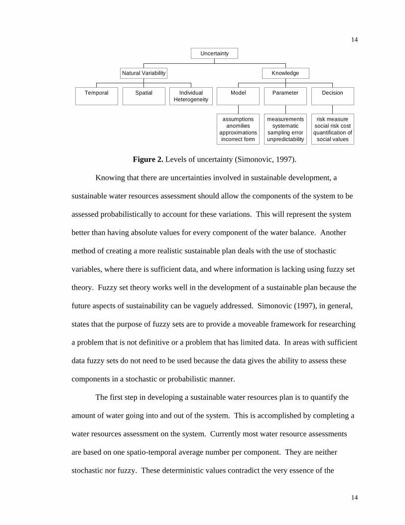
Uncertainty can be broken up into two separate categories. The first category

deals with the natural variability in the hydrometeorological variables of interest. These

sources of variability include spatial, temporal, and individual heterogeneity. Spatial

variability deals with changes occurring from one location to another. Temporal

variability happens as values change with time. Individual heterogeneity in general

contains all the other variations that take place in a system. It should be noted that there

are multiple scales of this natural variability. The second category of uncertainty deals

with a basic lack of knowledge in certain aspects of a system. This lack of knowledge

comes from a lack of data, or limitations on the level of understanding. This can be seen

in the use of models, the value of obtained parameters, and personal decision making

(Simonovic, 1997). This tree of uncertainty can be seen in Figure 2.

14

14

Temporal Spatial IndividualHeterogeneity

Natural Variability

assumptionsanomilies

approximationsincorrect form

Model

measurementssystematic

sampling errorunpredictability

Parameter

risk measuresocial risk costquantification of

social values

Decision

Knowledge

Uncertainty

Figure 2. Levels of uncertainty (Simonovic, 1997).

Knowing that there are uncertainties involved in sustainable development, a

sustainable water resources assessment should allow the components of the system to be

assessed probabilistically to account for these variations. This will represent the system

better than having absolute values for every component of the water balance. Another

method of creating a more realistic sustainable plan deals with the use of stochastic

variables, where there is sufficient data, and where information is lacking using fuzzy set

theory. Fuzzy set theory works well in the development of a sustainable plan because the

future aspects of sustainability can be vaguely addressed. Simonovic (1997), in general,

states that the purpose of fuzzy sets are to provide a moveable framework for researching

a problem that is not definitive or a problem that has limited data. In areas with sufficient

data fuzzy sets do not need to be used because the data gives the ability to assess these

components in a stochastic or probabilistic manner.

The first step in developing a sustainable water resources plan is to quantify the

amount of water going into and out of the system. This is accomplished by completing a

water resources assessment on the system. Currently most water resource assessments

are based on one spatio-temporal average number per component. They are neither

stochastic nor fuzzy. These deterministic values contradict the very essence of the

15

15

inherent risks in sustainability. It was stated by Simonovic (1997) that because of the

uncertainties of future development and today’s processes, probabilistic approaches to

water resource assessments are superior to simple deterministic approaches. However,

based on this literature review, it does not appear that communities or researchers have

attempted a combined probabilistic approach to a water resources assessment. There has

been much discussion of sustainable issues but little quantification, and unless action is

taken to turn quantitative sustainability concepts into a reality, “sustainable development

will remain a trendy catchphrase for a few years, and then gradually fade away like the

earlier concept of eco-development (Biswas, 1994, p.112).” This gap between concepts

and applications in sustainable development adds to the need for this research. Herein,

sustainable water resources are defined using the ASCE definition as those water

resources that meet the obligations of the present and the future while maintaining the

hydrological, ecological and environmental soundness of the system.

WATER BALANCE

A water balance is an essential element in any type of planning for sustainable

water development or water management plan (Miloradov, 1995). A water balance is

simply described as a mass balance of water entering and leaving a given volume. This

water balance can be described as seen in Equation 1, where inflow is equal to outflow

plus the change in water storage. Inflow (I) represents all the water flowing into the

system, which is defined by a set control volume or physical boundaries. This term can

include surface water, groundwater, condensation and precipitation. Outflow (O)

represents the water flowing out of a system from surface water, groundwater,

evaporation, and transpiration. The change in storage (ΔS) deals with the change in the

16

16

amount of water held in the system for the time period being analyzed. This change is

storage occurs from variations of water content in the soils, as well as storage differences

in underlying aquifers.

SOI Δ+= (1)

Equation 2 is an expanded water balance equation, specific to a watershed. In this

equation, precipitation (P) and ground water inflow (GI) are the only input variables

since a watershed, by definition, does not usually have surface inflow. It can also be seen

that evaporation and transpiration have been combined as one outflow called

evapotranspiration (ET) because the lack of ability to accurately measure these individual

outflows separately. The difficulties in analyzing evaporation and transpiration will be

discussed later in Chapter V. Other outflows consist of surface runoff (RO), ground

water outflow (GO), and the change in storage (ΔS).

SGOETROGIP Δ+++=+ (2) The water balance equation is the traditional method of determining the quantity

of water available for use in a system. A more complete approach of assessing water

resources towards sustainable development, which includes human water withdrawals

and discharges in the mass balance equations, where the first one ignores these elements,

is a water resources balance (Miloradov, 1995). This implies that water can be used

multiple times as it travels through the given watershed. The difference between a

conventional water balance, and a water resources balance can be seen in Figure 3.

17

17

Additionalwater available

for use

Precipitation

Surface Waters

Runoff

Water available for use

Groundwaters

Precipitation

Surface Waters

Runoff

Water available for use

Groundwaters

Lost water

Lost water

Basic Water Balance Approach

Water Resources Balance Approach Figure 3. Water balance and water resources balance (Miloradov, 1995).

The top flow chart in Figure 3 depicts a standard water balance and its internal

operations on a watershed scale. The system starts with an input of precipitation.

Precipitation then either falls on land or water. If it falls on land it will start to runoff.

This runoff can either infiltrate to groundwater, runoff the ground surface and form

surface waters, or it can return to the atmosphere through evapotranspiration and fall to

the earth again as precipitation. Surface water and groundwater interact with each other

in the forms of seeps, springs, stream baseflow, lakes, and possible high infiltration areas.

These two components also can have some loss of water in the form of

evapotranspiration back into the atmosphere. All water not lost through

evapotranspiration processes theoretically could be available for use. After this water is

used it is then lost to down stream areas and cannot be used in the watershed again.

18

18

The lower flow chart depicts a situation that encompasses the human interaction

that could take place in a water resources area. This water resources flow chart starts as

precipitation and moves down to either surface water or groundwater in the same manner

as the water balance chart. After the water is consumed and lost downstream humans

then collect a portion of this lost water and redistribute it back into the watershed as

either surface water or groundwater. This collection and redistribution of water allows for

it to be used twice or more thus allowing for an increase in the amount of water available

for use.

The water resources balance equation takes into account the same variables as the

water balance equation, but then adds to it the additional withdrawals and inflows from

human use. The water resources balance equation is represented in Equation 3. This

equation states that ΔS is equal to the natural inflow minus the natural outflow plus the

human inflow (HI) minus the human outflow (HO). This equation represents other

equations and mass balances within the system such as an independent balance solely for

surface water and another for ground water. And then these equations can be further

broken down into equations that contain components that can be directly measured and

those that cannot (Miloradov, 1995).

HOHIOIS −+−=Δ (3)

The accuracy that can be obtained for each component of the water resources

balance depends on the understanding of the process, the model being used to represent

that process, and amount of available data. Precipitation and surface runoff are simpler

and better understood compared to evapotranspiration, which is very complex and

dependent upon many other variables. Every model has certain inherent assumptions

19

19

used to simplify a process, and can only be applied accurately when these assumptions

are valid. Longer data records usually means that particular component will be more

representative of the natural component. Components with little available data have an

increased uncertainty since they cannot be patterned as effectively.

Precipitation

Precipitation is one of the directly measured components of the balance that

usually has an extended record longer than others. The problem with estimating

precipitation amounts is that precipitation is extremely spatially and temporally variable,

and historically measurements are made at only a few locations (if any) within a given

watershed. From the leeward to the windward side of mountains to the base and peak of

mountains, from winter to summer precipitation constantly varies depending on the

location, elevation and time of year. This causes uncertainty in the quantitative estimates

because most watersheds have a limited number of precipitation gages.

Today there are numerous methods of depicting and accounting for spatially

distributed precipitation. One of the older and more simplified methods is the Theissen

method. This method uses a map view of the area and connects adjacent precipitation

gages with a line. Perpendicular bisecting lines are then drawn on the map to form

polygons around each gage. These polygons then represent the appropriately sized area

to represent each gage that is encompassed. Two similar, older methods are the isohyetal

and isopercentual method. These methods are simply contour lines of equal precipitation,

or percent of average precipitation, respectively (Bloomsburg, 1959). They are created in

the same manner as an elevation contour map, by using the precipitation value and

location of each gage. There are, however, many ways of interpolating between the gage

20

20

locations. A number of these interpolation methods including the Kriging, universal

Kriging, first and second order polynomial, and reciprocal distance are discussed and

evaluated by Tabios (1985). From this paper Tabios (1985) concluded that the Kriging

methods performed the best based in relation to his performance criteria.

With the advances in technology, computers are playing an ever-increasing role in

the evaluation of precipitation. Computer programs based on advanced interpolation

techniques are now being used to calculate, display and model the spatial variability of

precipitation. Some precipitation models currently used in throughout the nation are

PRISM, MTCLIM-3D, and ANUSPLIN. These models create gridded precipitation

maps from point observations at gage locations along with digital elevation models

(DEMs) (Stillman, 2003). Stillman (2003) compared the results of these three models in

a study area surrounding Bozeman, Montana. It was shown that these models were not

statistically different when compared to the observed data. ANUSPLIN seemed to

overestimate the precipitation and also had the largest mean absolute error (MAE).

MTCLIM-3D tended to have higher precipitation values during the winter and early

spring and PRISM over predicted precipitation during the summer months (Stillman,

2003). All these methods seem to provide reasonable precipitation estimates, and are

more user friendly compared to the tedious hand methods. The ability to access the

information from these programs with geographic information systems (GIS) also makes

it more attractive to the modern day user. The PRISM model, however, is more widely

known and accessible. Questions also arise on the transferability and effectiveness of the

ANUSPLIN and MTCLIM-3D models. As part of the PRISM project, precipitation maps

21

21

for the entire US based on 30 year average precipitation values have been created. The

PRISM maps were chosen to be used herein due to these factors.

Evapotranspiration

Evapotranspiration is one of the major outflow components in a water resources

balance. It is also one of the hardest components to determine accurately. For ages this

hydrologic process has been studied, and is still difficult to quantify the amount of daily

or monthly evapotranspiration. Evapotranspiration is difficult to quantify because it is

affected by spatial variations in climate, terrain, vegetation, and soil composition (Biftu,

2000). In vegetated areas, such as the Palouse, evapotranspiration is more complicated

because the vegetation and canopy cover are continuously changing throughout the year.

The earliest method developed to determine evapotranspiration was created by

Penman. This method uses a modified energy balance equation to estimate the amount of

evaporation from open water surfaces (McCuen, 1998). Since it was developed, many

people have modified the Penman equation in order to represent a naturally vegetated

area or crop. One of the more popular modified equations is the Penman-Monteith,

developed by Monteith (1965), which takes into account a canopy resistance factor. The

Penman equation was altered from its original form to account for different non-saturated

land covers (Biftu, 2000). When the canopy resistance is assumed to be zero in the

Penman-Monteith equation, the result is the Priestley-Taylor equation.

There are numerous other models that try to represent evapotranspiration. All of

these methods have different assumptions or are based on different conceptualizations of

the ET process. One of these is the Jensen-Haise method, which relies on the assumption

that solar radiation is the most important factor in evapotranspiration. In 1968,

22

22

Christiansen tried to relate pan evaporation to evapotranspiration, as many people since

then have also tried (Davis, 1971). McNaughton and Black modified the Priestley-Taylor

equation to be used in a Douglas fir watershed where canopy height is greatly increased

when compared to croplands (Cherry, 1986). Other models were developed by Blaney

Criddle, Thornthwaite and Mather, and Rich (Bloomsburg, 1959).

Hargreaves method is also commonly used to estimate ET on a time step usually

longer than one day, although daily time steps are frequently used. A study conducted by

Wu (1997) concluded that comparing 1 day ET estimates to measured ET versus a 7 day

moving average for each ET resulted in Nash-Sutcliffe values improving from 0.6 to 0.9

for the Hargreaves method. It was increased even further with a 15 day moving average,

indicating that this method is more suitable to larger time scales. It is also the easiest

model to use for practical purposes. The two minor input parameters temperature, and

solar energy are readily available throughout the world (Wu, 1997). The Hargreaves

method uses the minimum and maximum temperature for the established time step along

with the latitude and Julian day or month of the year to calculate the solar energy

available. Hargreaves equation consistently produces accurate estimates of potential

evapotranspiration (as measured using energy balance techniques, the Penman

combination equation, or lysimetric observations), and in some cases, much better than

estimates made using more complex methods (Hargraeves, 1982; Mohan, 1991; Saeed,

1986).

Today the two main methods, besides satellite imagery, for calculating ET are the

Penman-Monteith and Hargreaves models. In this analysis the Hargreaves method was

used rather than the Penman-Monteith equation because of lack of historical input data

23

23

for the PM equation and the ability of Hargreaves to accurately estimate ET. Mohan

(1991) also found the Hargreaves equation to be highly correlated with the Penman

combination equation for estimates of average weekly evapotranspiration.

Surface Runoff

If precipitation is not infiltrated into the ground it will runoff on the surface

according to topography. Surface runoff is created either by the infiltration excess and

the saturation excess mechanisms. Infiltration excess (or Hortonian) overland flow is

runoff caused by soil saturation from above. This type of overland flow is caused when

the infiltration capacity of the ground is less than the rainfall intensity. If any slope

exists, the water will start to flow overland. Saturation excess overland flow is caused by

soil saturation from below. This occurs when the groundwater table rises to the ground

surface level, causing surface ponding and overland flow (both from exiting groundwater

and falling precipitation). As water flows downhill it conglomerates in low elevations

where it will channelize and flow into a stream or river.

There are numerous ways to determine the stream flow rate at a given time. The

Natural Resources Conservation Service (NRCS) has a “rule of thumb” equation to

determine the annual discharge that has proven fairly accurate where annual rainfall is

greater than 30 cm, but is very elementary (Bloomsburg, 1959). Fixed structures in the

channel are often used for extended discharge measurements. These structures could be

any type of weir (e.g., a broad crested weir) where the height of water above the weir

crest corresponds to a certain flow rate. These flow rate calculations are based on the

conservation of energy and momentum. Other types of permanent measurement

structures include orifices, flumes, and culverts.

24

24

If there is no permanent discharge measuring structure located at a site, the most

effective method to determine the discharge is to measure velocity at a stream cross

section. This cross section should be the perpendicular bisector to the main flow path in

a channel. A person then measures the water depth, and flow velocity at numerous

locations along this cross-section. To obtain a representative velocity, flow velocity

measurements are usually measured at sixty percent of the total water depth at each

location. If water depths exceed 60 centimeters in depth the average of the velocities

measured at the 80% and 40% depths should be used. These velocity measurements are

then multiplied by their depth and sectional width to obtain sectional discharges; when

added together the result is the total discharge. Discharge measurement accuracy will

increase as the number of velocity measurements made through the width of the channel

increases.

The most common method of measuring stream flow continuously relies on using

pressure transducers in the bottom of channels. These pressure measurements are related

to a depth of water. The depth of water is in turn related to the discharge, which was

measured by taking cross section measurements. This relationship between stage and

discharge is called a rating curve. This allows for continuous monitoring of stream flow.

As with precipitation, the longer the record the more accurate the computed temporal-

average discharge volumes will be.

Surface runoff is measured at a point. This non-distributed approach is sufficient

for water balance assessments since the main interest of quantifying surface runoff is

where the stream or river exits the watershed boundary. This measurement does not

provide any information about the spatial distribution of discharge above the

25

25

measurement location. If a semi-distributed approach is desired flow measurements

would have to be made where tributaries fed into the main channel. This allows sub-

basins of the watershed to be analyzed for their individual contributions to surface runoff.

Groundwater

When water infiltrates into the soil it turns into groundwater. Groundwater can be

thought to exist in two different forms. Groundwater will often exist and flow in

unsaturated areas. This type of flow existing below the surface and above the regional

water table is often referred to as interflow or throughflow (Dingman, 2002). Interflow

occurs in fine-grained soils where pore sizes are small enough to suspend the

groundwater in tension (negative pressure). This type of flow is often described as

Darcian flow in the soil matrix, or as macropore or pipe flow (Dingman, 2002). The

other type of groundwater is saturated groundwater, where all the pore spaces are filled

with water. This top level of this type of groundwater is referred to as the water table.

Both saturated and unsaturated groundwater flows through the soil moving from high to

low head areas as described by Darcy’s Law.

Geologic units of saturated groundwater that are capable of producing

economically viable volumes of water are called aquifers. Aquifers can be either

confined or unconfined. When the groundwater surface is at atmospheric pressure, the

flow and aquifer are considered to be unconfined (Marsily, 1986). A confined aquifer

occurs in nature when the aquifer is restricted from above by a soil layer with a very low

saturated hydraulic conductivity called a confining layer. This restrictive soil layer

induces a pressure on the aquifer such that the water level in an observation well will rise

above the confining layer to a level equal to the potentiometric surface (Dingman, 2002).

26

26

There are many models and methods of determining groundwater flow and the

recharge that is occurring in a system. Some of the more popular methods are 1-D, 2-D,

3-D, and other mathematical models (Lum, 1990; Simmers, 1987; Smoot, 1987). Other

methods include the Hill method and zero water change method (Baines, 1992). Methods

that are becoming more popular are tritium injection studies as well as other

environmental tracer studies (De Vries, 2000; O'Green, 2002; Rangarajan, 2000;

Simmers, 1987). Due to the complexity of the groundwater system underlying the

Moscow-Pullman area these methods were not utilized and basic assumptions were made

on groundwater movement.

The hardest components of a water resources balance to quantify are those which

occur underneath the ground. Groundwater movement, volume and recharge are difficult

aspects of the water resources balance to quantify, because they cannot be seen or

monitored easily. Even accurately monitoring the amount of water humans withdraw

from groundwater sources becomes difficult when all municipal and private wells are

combined. Difficulties also arise when computing natural basin groundwater outflow and

inflow. The uncertainty in the shape of aquifers also confuses the issues underground

and only educated guesses can be made as to what is actually occurring underneath the

ground. The scope of this work does not deal with the necessity to analyze the shape,

formation, and volume of the aquifers.

27

27

CHAPTER III

METHODS

A probabilistic water resources assessment of the Paradise Creek Watershed will

help move the Palouse region towards a sustainable water management plan. Currently

groundwater is the sole source of regional domestic water. Figure 4a, depicts the current

situation. This flow chart shows how precipitation may turn to surface water or

groundwater once it falls to earth. Water can go back into the atmosphere through

evapotranspiration, or stay in groundwater or surface water, keeping in mind that these

two systems interact throughout the watershed. Groundwater then goes towards human

use, or it flows out of the watershed. All surface water currently flows downstream, and

out of the watershed.

To move the region towards a sustainable water resources plan, a new water

assessment is necessary. This new water balance can be seen in Figure 4b. The main

difference in this water balance compared with the old balance is the application of

surface waters. In the current case nosurface water is utilized and flows out of the

watershed for use by downstream consumers. This new balance allows surface water to

be used by humans. The purposed use of surface water will reduce dependency on

groundwater, and in turn curb the current aquifer depletions taking place. The new water

resources assessment will be probabilistically quantified through the use of historical data

and mathematical models to determine its applicability to the region under consideration.

28

28

Precipitation

Groundwater Surface Water

Water ForUse

ETET

Lost Water

a. Current water resources balance.

Precipitation

Groundwater Surface Water

WaterForUse

Lost Water

ET ET

b. New water resources balance. Figure 4. a. The current water resources balance. b. New water balance for sustainable water resources management.

29

29

The water balance is cast in a probabilistic format on an annual basis using readily

available data to address the uncertainties involved in sustainable water resources

management. Equation 4 shows the water balance that was applied to the watershed.

Each variable within this equation is represented by its own probability of exceedence

function (PEF). The PEFs that can be determined from data analysis and modeling can

be combined to develop a probability of exceedence function for the amount of deep

percolation occurring. This equation also aids in the determination of the quantity of

water that can be used for human consumption and use. The use of these probability

functions for each component of the water balance brings together the use of old

established methods with the increasing use of more complex statistical formulas to

create a new technique to more accurately assess the uncertainties in water resources.

GIGODPETSRP −+++= (4)

All terms in Equation 4 are determined from historical data and modeling

techniques except for deep percolation and groundwater inflow and outflow. Deep

percolation is defined as the drainage of water beyond the root zone (Hillel, 1982). This

value is currently unknown to a useful degree of accuracy for the study area.

Assumptions were made on groundwater flow through the aquifers to add these

components into the water resources assessment.

Precipitation data were obtained from a spatial and temporally distributed model,

PRISM, as well as data from a local weather station. Surface runoff was determined

from a stream gage at the outlet of the watershed along with other gages located

throughout the watershed. Local water withdrawals were determined from well logs, and

data obtained from PBAC.

30

30

The water resources assessment utilized a yearly time step for each component of

the water balance. The use of a yearly time step simplified the water balance equation by

eliminating the snow water and soil water storage components since on a yearly average

these values will be zero (Cherry, 1986). This assumption is valid assuming that there

are no climatic trends. A yearly time step was used rather than a monthly or daily step

due to lack of information dealing with soil and snow storage. However, monthly

probability functions were created for precipitation, surface runoff, human withdrawals,

and evapotranspiration for use later when soil storage data becomes more available for

the watershed.

Historical data used for the water resources balance was obtained from two

distinct sources. Historical surface runoff data was obtained from a USGS stream gaging

site located just upstream from where Paradise Creek exits the watershed. This site has

24 years of daily discharge data available. The other source of historical data came from

a weather station located approximately 1km east of the southern tip of the watershed. At

this weather station precipitation as well as minimum and maximum temperatures were

used for this water resources assessment. These were the only two sites located in close

proximity to the watershed that were used for this analysis.

Precipitation, surface runoff, evapotranspiration, and groundwater withdrawal

amounts all were computed using historical data. The period of historical data used for

all components is from 1979-2002. This period of record was limited by the available

surface water data. There were longer data records for precipitation, evapotranspiration,

and groundwater withdrawals, but due to the short record of surface runoff the historical

records of the other parameters had to be cut short. The use of a uniform historical period

31

31

is necessary to represent each component with the same statistical background. This

eliminates the possibility of certain components being affected by climate change, and

other long term trends creating a misrepresentation of these parameters. The creation of

the historical evapotranspiration utilized historical minimum and maximum daily air

temperatures in the Hargreaves model. This created historical evapotranspiration records.

The mean areal average precipitation obtained from the PRISM data was

corrected using historical data from a nearby weather station maintained by the

University of Idaho. Since the PRISM maps are based on a 1961-1990 average the map

had to be corrected to fit the time period of 1978-2002 for the water balance being

conducted. The PRISM data were corrected for time by multiplying it by the ratio

between the 24 year and 30 year historical data averages as seen in Equation 5.

Correcting the PRISM data by this ratio resulted in the mean areal precipitation for the 24

year record ( 24AP ) used in this study. The 24 year average areal precipitation value then

needed to be desegregated to each separate year to obtain the areal precipitation for that

year ( yAP ). This was done using another ratio between the historical year’s precipitation

and the 24 year average precipitation as seen in Equation 6. The data was not corrected

for the difference between the 30 year historical average and the PRISM value for that

location because the relative error was less than 2.5%. These correction factors along

with average precipitation values can be seen in Table 1.

⎟⎟⎠

⎞⎜⎜⎝

⎛=

30

2424 *

PP

PRISMAP (5)

⎟⎟⎠

⎞⎜⎜⎝

⎛=

2424 *

PP

APAP yy (6)

32

32

Table 1. Average precipitation values and historical scale factors.

Surface waters used historical data available from a USGS stream gaging site

located approximately where the surface water exists the watershed.

To obtain the potential evapotranspiration (PET), in centimeters that had occurred

throughout the watershed the Hargreaves method was used. The Hargreaves PET

equation that was used is seen in Equation 7. The Hargreaves method requires minimum

and maximum temperatures, in degrees Celsius, for the designated time step as well as a

potential radiation factor (PR). Equation 8 is the lambda factor that needs to be used in

the determination of the potential evapotranspiration. This method also requires the

latitude and Julian day to determine the potential radiation. The solar energy is

determined from these input parameters as seen in Appendix A. PET was determined on

a monthly and annual time basis and added to form yearly PET estimates.

( ) ( ) ( )λ*100/**8.17*0023.0 5.0minmax PRTTTPET −+= (7)

T*002361.0501.2 −=λ (8)

Time Time Spatial Historical DataPeriod 24 year 30 year PRISM Scale Factor Scale Factor Scale Factor

January 7.17 7.91 8.61 0.906 1.201 1.089February 6.37 5.77 6.38 1.104 1.002 1.106March 6.57 6.1 6.55 1.077 0.998 1.075April 6.68 5.48 5.78 1.219 0.865 1.054May 6.55 5.68 5.98 1.153 0.913 1.053June 4.89 4.51 4.89 1.084 1.000 1.084July 2.86 2.38 2.49 1.202 0.872 1.048August 2.82 2.94 3.15 0.959 1.115 1.070September 3.34 3.24 3.50 1.031 1.049 1.081October 5.52 4.69 4.87 1.177 0.882 1.038November 9.15 8.29 8.83 1.104 0.966 1.066December 7.34 7.46 8.47 0.984 1.153 1.135

Annual 68.83 64.46 69.08 1.068 1.004 1.072

Average Precipitation Values

33

33

The historical values were then fit to a statistical distribution to create probability

density functions (PDF) as well as probability of exceedence functions. The statistical

distribution used on all historical data was the Log Pearson Type III (LPIII) distribution.

The Log Pearson Type III distribution is the standard distribution used for flood

frequency analysis within the US (Benson, 1968; WRC, 1982). This distribution is the

log form of the Pearson Type III distribution or the three parameter gamma distribution.

The LPIII distribution is suited well to frequency analysis where data are significantly

positively or negatively skewed (Chow, 1988). The LP3 distribution creates PEF’s from

the use of Equation 9. Equation 9, describes how the value at a specified exceedence

probability (xep) is dependent upon the average ( x ), standard deviation (σ), skewness of

the historical data (Cs), and the desired exceedence probability. The average is added to

the product of the standard deviation and the frequency factor (KT). The KT factor is

determined from tables or approximated as described in Equations 10-12, and is a

function of the standard normal variable (z) and the skewness (Cs).

σ*Tep Kxx += (9)

6/sCk = (10)

( ) σ/xxz ep −= (11)

( ) ( ) ( ) 5432232 *3/1**1**6*3/1*1 kkzkzkzzkzzKT ++−−−+−+= (12)

Deep percolation was determined using a derived distribution analysis. This was

done by converting the probability distribution functions for each component into their

respective cumulative distribution function (CDF). The CDF’s are a function of depth,

and to derive the CDF for deep percolation the functions needed to be converted to

functions of cumulative probability, which was done by taking the inverse of the CDFs.

34

34

Adding and subtracting the appropriate values of precipitation, surface runoff, and PET

from the inverse CDF’s created the inverse cumulative distribution function for deep

percolation. This can be seen in Equation 13. This equation states that the inverse of the

cumulative distribution functions ( ( )xF ) can be directly added and subtracted together.

In this equation the subscripts specify the specific component and “x” is depth. From

Equation 13 the deep percolation CDF curve can be turned into a probability of

exceedence function and used easily with the rest of the results.

( ) ( ) ( ) ( ) 1111 −−−− −−= xFxFxFxF ETSRPDP (13)

All components of the water balance and the human consumption are combined in

the end to assess the water resources and determine the sustainability of the system for a

given year. This was done by determining the water available for human consumption

and dividing it by the actual water used for human consumption to form a simple ratio of

available to actual water consumed. If the ratio is greater than or equal to one the system

is deemed sustainable. If the ratio is less than one the system is determined to be

insufficient for the given year and water must be pumped out of the Grande Ronde

aquifer utilizing the Grande Ronde’s safe yield, which has not been determined, or

creating an unsustainable system.

Surface water quality was also analyzed since it is a critical component in any

water resources assessment (Goodwin, 1990). Water quality was evaluated throughout

the watershed at established stream gaging locations. Water quality parameters were

evaluated and relationships were derived to ease in future testing. Fast and economically

measured water quality parameters were correlated to more time consuming and

expensive water quality tests to allow easier monitoring of various quality parameters.

35

35

Various water quality parameters were also compared to and correlated with water

quantity. This shows how water quality varied spatially and temporally dependent upon

surface runoff.

The compilation of the water quality data was gathered through use of various

sampling methods. The two lower gages of the three new permanent gaging stations

located along Paradise Creek, as seen in Figure 5, have the capabilities to continuously

monitor turbidity, electroconductivity, and temperature. These stations also incorporate

ISCO samplers to obtain water samples for further testing. These samples can be taken at

specified time intervals or with designated changes in stage. These water samples were

then taken back to the laboratory and tested for total suspended solids, and turbidity. A

depth integrated sampler, as well as grab samples were used to test for nitrates, and

coliforms at the gaging stations. Historical water quality data on Paradise Creek gathered

from local Idaho Alliance of Soil Conservation District (IASCD) studies were also used

for electroconductivity, nitrates, turbidity, total dissolved solids, pH, and phosphorous

testing. The location of these IASCD water sampling sites can be seen in Appendix B.

These water quality results were obtained from the IASCD’s 2001 and 2002 yearly

reports on Paradise Creek (Myler, 2002).

Samples were tested on site and in laboratory settings. Table 2, shows the

instrument and or testing method used on obtained samples and continuously monitored

parameters.

36

36

MWWTP

USGS

Darby

Hawley

Figure 5. Locations of gaging stations.

Parameter Method/Instrument

Orion Model 115Cambell Scientific CS 547

Nitates EPA 300.0pH Orion Model 210APhophorus EPA 365.2Temperature Cambell Scientific CS 547Total Coliforms Standard Method 9221BTotal Dissolved Solids Orion Model 115Total Suspended Solids EPA 160.2

Hanna Instruments 93703D&A Instruments OBS-3Turbidity

Electroconductivity

Table 2. Water quality testing methods/instruments.

37

37

CHAPTER IV

WATERSHED DESCRIPTION

The Paradise Creek Watershed consists of the surrounding area encompassing

Paradise Creek located in Idaho. Paradise Creek is a fourth order stream that originates

on the southwest side of Moscow Mountain approximately 13 kilometers north of

Moscow, Idaho. This stream flows off Moscow Mountain, heading south, and meanders

through the rolling hills of the Palouse until it reaches Moscow, Idaho. From Moscow,

the Creek heads west towards Pullman, Washington, where it joins the south fork of the

Palouse River. For this study the lower watershed boundary is defined where the

Moscow Wastewater Treatment Plant stream gaging site is located or roughly the Idaho-

Washington State line boundary. A digital elevation map of the watershed can be seen in

Figure 6. Paradise Creek watershed has a peak elevation of 1320 meters. Where it exits

the watershed Paradise Creek is only at an elevation of 775 meters. The mean elevation

from the hypsometric curve in Figure 7 is 835 meters. The area of the watershed is 45.6

square kilometers. This area is used for all conversions between depths of water and

volumes.

38

38

Figure 6. Digital elevation model of Paradise Creek watershed.

700

800

900

1000

1100

1200

1300

1400

0% 10% 20% 30% 40% 50% 60% 70% 80% 90% 100%% of Total Area

Elev

atio

n (m

)

Figure 7. Hypsometric curve of Paradise Creek watershed.

39

39

The major types of soil found on the watershed consist of some type of a

moderately to well drained silt loam formed in loess (Barker, 1981). Loess is a soil that

is wind transported from glacial till and end moraine deposits. Underlying these loam

soils are two layers of basalt. The upper basalt layer comes from the Wanapum basalt

flows, while the deeper thicker basalt layer was formed from Grande Ronde basalt.

Moscow Mountain and the upper extents of the watershed are characterized by a granitic

outcropping. This outcropping dives underground and is covered by the typical silty

loam near the base of Moscow Mountain. In some soil types a fragipan exists underneath

the top 0.5 to 1.0 m of loose soil causing perched water tables in winter and spring (Boll,

2003). This fragipan is comprised of a hard clay layer (Brooks, 2000).

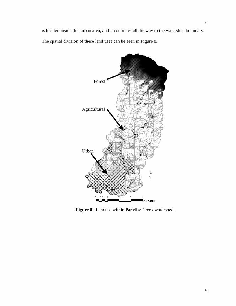
The watershed is readily divided up into three distinct areas based on land use. In

the upper portion of the watershed, coniferous trees are the dominating vegetation. These

forests primarily consist of Ponderosa Pine, Spruce, Douglas Fir, White Fir, Western

Larch, White Pine, and Cedar, with a considerable amount of native undergrowth (e.g.

Thimble Berry, Snow Berry, Oregon Grape) (Bloomsburg, 1959). This forested area

roughly comprises 14% of the total watershed area. Below the forested area the

watershed serves agricultural purposes. The majority of this area is used for the

production of winter wheat, alfalfa, and legumes, as well as blue grass for minor

livestock grazing. The agricultural area is the largest of the three subdivisions in the

watershed, occupying 69% of the land. As Paradise Creek moves down through the

agricultural area it migrates into the urban area. This area takes up approximately 17% of

the watershed area and is located on the bottom one third of the stream’s length. Moscow

40

40

is located inside this urban area, and it continues all the way to the watershed boundary.

The spatial division of these land uses can be seen in Figure 8.

Urban

Agricultural

Forest

Figure 8. Landuse within Paradise Creek watershed.

41

41

CHAPTER V

RESULTS

This chapter addresses each component of the water resources assessment. At the

end of this chapter all components will be conglomerated into the final water resources

assessment. All results are presented as equivalent depths of water over the entire

watershed. This will lead to a discussion on human consumption and, and finally

recommendations for management practices are presented.

PRECIPITATION

The Paradise Creek Watershed has a high temporal and spatial variation in

precipitation. Precipitation is highest during December and January, while it is lowest

during August. The major portion of precipitation falls as snow or a combination of

snow and rain. Low intensity rain and snowfall events from November through January

account for 40% of the yearly precipitation (Boll, 2003).

The precipitation data for use in this probabilistic water resources assessment

comes from various sources, as discussed previously. The main source of precipitation

data are the distributed PRISM maps. This statistical-topographical model used to create

the PRISM maps utilizes weather station data from 1961-1990, which are transformed

into a nation wide precipitation grid map with a 2 km grid resolution. The spatial

distribution of average annual precipitation for the watershed can be seen in Figure 9.

Monthly maps are also available. These average precipitation values were integrated

over the watershed area and then converted into a mean areal precipitation. A

42

42

probabilistic exceedence function was created from this average precipitation data when

combined with historical variations in precipitation, as described in Chapter III.

Figure 9. Distribution of annual average precipitation.

The probabilistic precipitation analysis for the watershed quantifies uncertainties

due to natural variability of the monthly and annual precipitation volumes. The PEF of

annual precipitation using the LPIII distribution function can be seen in Figure 10 and is

bounded by the upper and lower 95% confidence intervals (CI). Table 3, shows select

average monthly and annual precipitation depth (cm) probabilities for the watershed. The

historical data and monthly values can be found in Appendix A. These integrated

average precipitation values are the basis for the remaining components of the water

balance.

43

43

Figure 10. Probability of exceedence of annual precipitation based on the LPIII

distribution function.

Probability 0.99 0.5 0.2 0.1 0.04 0.02 0.01 0.002Return Period (yrs) 1.0 2 5 10 25 50 100 500Annual 46.63 67.40 78.84 86.01 94.76 101.11 107.34 121.69January 1.25 8.76 12.05 13.39 14.44 14.92 15.24 15.63February 1.75 5.48 8.67 11.13 14.65 17.56 20.74 29.29March 0.98 6.92 8.89 9.50 9.88 10.01 10.08 10.14April 1.45 5.29 7.89 9.59 11.69 13.22 14.71 18.07May 1.40 5.65 8.19 9.68 11.37 12.49 13.50 15.55June 1.00 4.62 6.80 8.07 9.46 10.36 11.16 12.72July 0.10 1.86 4.03 5.73 8.02 9.77 11.51 15.47August 0.01 1.90 5.88 9.25 13.68 16.82 19.71 25.30September 0.05 2.68 6.15 8.48 11.10 12.74 14.12 16.49October 0.19 4.84 7.56 8.58 9.27 9.54 9.69 9.84November 2.09 8.65 11.95 13.67 15.39 16.42 17.28 18.78December 1.27 7.75 12.22 14.93 18.01 20.05 21.89 25.54

Precipitation Probability of Exceedence (cm)

Table 3. Exceedence probabilities for precipitation over the watershed.

SURFACE RUNOFF

Water flows in Paradise Creek throughout the year. As with most Pacific

Northwest streams peak flows occur during the spring snowmelt from February to May.

Paradise Creek experiences low flow conditions in July through September where the

10

100

1000

Probability of Exceedence

Ann

ual P

reci

pita

tion

(cm

)

.99 .98 .95 .90 .70 .50 .30 .10 .05 .02 .01

44

44

majority of flow is baseflow and does periodically completely dry up in the upper third of

the watershed.

The surface runoff exits the defined watershed at the Moscow Wastewater

Treatment Plant (MWWTP) gaging station operated by the University of Idaho. This

specific gage only has 1.5 years of stream flow data. However, the USGS stream gage

13346800 located where Paradise Creek exits the University of Idaho property has 24

years of daily discharge measurements. The close proximity of these two gages allows

the historical values obtained from the USGS gage to be directly used without the need to

correct and regress the MWWTP gage’s data.

This historical data were reduced and compiled into monthly probabilistic

distributions using average monthly flow data from the 24 years of regressed data.

Figure 11, shows the probability exceedence function of annual surface runoff bounded

by the 95% confidence intervals. Monthly and annual data for specified probabilities are

displayed in Table 4. More data on monthly flows can be found in Appendix A.

1

10

100


Ann

ual D

isch

arge

(cm

)

.99 .98 .95 .90 .70 .50 .30 .10 .05 .02 .01

Figure 11. Exceedence probability of annual discharge.

45

45


Probability of Exceedence of Discharge (cm)

Table 4. Exceedence probabilities for discharge from the watershed.

EVAPOTRANSPIRATION

Evapotranspiration is the most difficult surface component of the water balance to

quantify. The difficulty in accurately representing this component is explained by the

complexity of the evaporation and transpiration processes. These processes are

dependent upon a multitude of variables many that cannot be accurately measured in the

field.

Evaporation measurements from an evaporation pan have been made daily at the

weather station being used. These data have been gathered for over 30 years. These pan

evaporation data were going to be used as an aide in the evapotranspiration calculations,

but were not used due in part to the lack of a reasonable correlation between monthly pan

evaporation and average monthly temperature. Also, pan evaporation is known to be a

poor estimator of evapotranspiration in dry land farming areas, especially where high soil

tensions (low moisture contents) are found in the watershed (Davis, 1971).

Minimum and maximum temperatures were obtained from the weather station and

used to compute historical potential evapotranspiration data. The latitude used in these

46

46

calculations was the mean latitude of 46o 47’ 19”. A distributed latitude was not used for

ease of calculations. This assumption of one average latitude resulted in possible errors

of plus or minus 0.5%. This small error is deemed insignificant.

To obtain the corrected potential evapotranspiration the PET had to be multiplied

by a crop coefficient. To account for the entire watershed and variability in land use and

cover a semi-distributed crop coefficient was applied. From the land use map seen in

Figure 8 the total area was broken up into various percentiles of urban, agricultural, and

forest land. The agricultural land was then broken down into more distinct food plots of

wheat, legumes, grazing, etc. The urban area was considered to be 80% houses,

buildings, etc, while the remaining 20% was considered to be short grass. The forest was

assumed to be composed of 80% forests and 20% brush, which is representative of the

surrounding areas. Table 5, shows the individual crop coefficients used for each distinct

land use. These values were obtained from Allen (1998). These values were then

multiplied by their respective areal percent and added together to form the semi-

distributed crop coefficient. This formula can be seen in Equation 14.

Jan. Feb. Mar. Apr. May June July Aug. Sep. Oct. Nov. Dec. Annual0.36 0.36 0.60 1.00 1.00 1.00 1.00 0.96 0.84 0.84 0.36 0.36 0.72

Coniferous 0.40 0.40 0.60 1.00 1.00 1.00 1.00 1.00 1.00 1.00 0.40 0.40 0.77Brush 0.20 0.20 0.60 1.00 1.00 1.00 1.00 0.80 0.20 0.20 0.20 0.20 0.55

0.28 0.28 0.28 0.48 0.48 0.50 0.50 0.50 0.48 0.28 0.28 0.28 0.39Houses 0.20 0.20 0.20 0.20 0.20 0.20 0.20 0.20 0.20 0.20 0.20 0.20 0.20Grass 0.40 0.40 0.40 0.90 0.90 0.95 0.95 0.95 0.90 0.40 0.40 0.40 0.66

0.28 0.36 0.52 0.74 1.01 1.10 1.10 0.53 0.45 0.28 0.28 0.28 0.58Barley 0.25 0.25 0.25 0.50 1.00 1.15 1.15 0.40 0.25 0.25 0.25 0.25 0.50CRP/Fallow 0.40 0.40 0.40 0.80 0.80 0.85 0.85 0.80 0.80 0.40 0.40 0.40 0.61Legumes 0.20 0.20 0.20 0.40 0.80 1.15 1.15 0.55 0.20 0.20 0.20 0.20 0.45Pasture 0.40 0.40 0.40 0.70 1.00 1.00 1.00 1.00 1.00 0.85 0.85 0.40 0.75Wheat 0.25 0.40 0.70 0.85 1.15 1.15 1.15 0.40 0.40 0.25 0.25 0.25 0.60

Forest

Urban

Agricultural

Crop Type

Table 5. Monthly crop coefficients for PET calculations.

47

47

∑

∑

=

== n

ii

n

iiT

total

A

AKK

i

1

1

* (14)

When monthly and yearly PET values had been estimated they were fit to the Log

Pearson Type III distribution as described earlier. The probability of exceedence values

bounded by the 95% confidence intervals for annual PET estimates can be seen in Figure

12. Table 6, contains monthly and annual ET values tabulated by various exceedence

probabilities. Complete monthly and annual records can be found in Appendix A.

Figure 12. PET probability of exceedence.

10

100


Ann

ual P

ET

(cm

)

.998 .99.98 .95 .90 .80 .70 .50 .30 .20 .10 .05 .02 .01 .005

48

48


Hargreaves PET Probability of Exceedence (cm)

Table 6. Monthly and annual PET probabilities of exceedence.

GROUNDWATER

For the initial water resources assessment many assumptions on the contribution

and movement of groundwater sources were made. Groundwater was broken into the

two different aquifer systems to ease the complications associated with quantifying

groundwater movement and interaction. This was done to separate distinctly different

aquifers. The main difference is that shallow aquifers have been noted to be influenced

by recharge while the deeper confined aquifer apparently has no significant form of

recharge and is hydrologically isolated from any current recharge sources (Murray,

2002).

Recharge in the Wanapum aquifer has been observed from well logs and water

table recovery. The Wanapum aquifer was assumed to consist of all groundwater sources

from the surface down to the Wanapum basalt, Grande Ronde basalt interface. This

includes the Wanapum aquifer, all crystalline aquifers, and any other shallow aquifer

systems in the loess. For this upper system it was assumed that groundwater flowed into

the system, at the same rate that it flowed out of the system in a lateral direction. All

49

49

possible recharge flowing into the Wanapum system is assumed to hold in the area for

possible human consumption. These are commonly made assumptions and are being

used here for preliminary purposes only and should be revised as more information

becomes available. All private wells in the area are assumed to extract water from this

system. The ability of the Wanapum to currently receive recharge makes it a more

sustainable water source than the Grande Ronde (Murray, 2002).

The Grande Ronde aquifer system was assumed to be confined with no recharge

occurring. This assumption is supported by the isotope dating of the water conducted by

Kent Keller and others as being 10,000 years old (Larson, 2000; O'Brien, 1996). It was

assumed that no inflow or outflow of water exists except for the human pumping that is

occurring. This aquifer is essentially modeled as a holding tank. Anything that is taken

out of it cannot be replaced. By the use of these assumptions the Grande Ronde is

theoretically mined whenever any water is extracted. Since this resource is not being

replenished it will not be evaluated for this water resources assessment, except as a

reserve of water for additional use during extended periods of drought.

SOIL MOISTURE

Soil moisture variations were not taken into account for this study. On a yearly

basis the change in soil moisture is considered to be zero. On a monthly basis this

assumption is violated. This factor was therefore only considered on an annual scale, and

no values were used for monthly interpretations.

DEEP PERCOLATION

Deep percolation was the only component of the water resources assessment for

which there was no historical data. It is assumed that all deep percolation is occurring in

50

50

the Wanapum system. To determine the PEF of deep percolation a probability

distribution was derived from the PEFs of the other components and water balance

equation. The derived distribution procedure used was discussed in Chapter III. Deep

percolation became a function of precipitation, surface runoff, and evapotranspiration.

The yearly PEF can be seen in Figure 13. Figure 13 and the upper and lower 95%

confidence intervals show the increased uncertainty of determining the deep percolation

from the other components of the water balance. These confidence intervals were

determined in the same fashion as the derived distribution except there are upper and

lower confidence intervals. To derive the correct upper confidence interval for deep

percolation the upper confidence interval for precipitation was used with the lower CI for

surface runoff and evapotranspiration, resulting in the highest deep percolation possible

for a 95% CI. Likewise for the lower confidence interval of deep percolation the lower

CI of precipitation was used with the upper CI of surface runoff and evapotranspiration.

By combining the uncertainties from precipitation, surface runoff, and

evapotranspiration, shown by their confidence interval bounds, the uncertainty of the

derived deep percolation in increased. Table 7, shows the deep percolation values as they

vary with different probability of exceedence values. By knowing the recharge occurring

to the shallow aquifer system the maximum volume available for withdrawal without

mining the aquifer could be determined.

51

51

Figure 13. Deep percolation probability of exceedence.

Probability 0.99 0.5 0.2 0.1 0.04 0.02 0.01 0.002Return Period (yrs) 1.0 2 5 10 25 50 100 500Annual 3.27 8.54 11.50 13.70 17.24 20.23 21.97 28.98

Deep Percolation Probability of Exceedence (cm)

Table 7. Annual deep percolation probabilities of exceedence.

WATER RESOURCES ASSESSMENT

With all the elements of the water balance determined and combined human

consumption can be added to create the complete water resources assessment. All

probability of exceedence functions for the water balance can be seen in Figure 14. From

these functions the water available for potential human consumption can be determined.

In the Moscow-Pullman area there are four major entities consuming water. These are

Moscow, Pullman, the University of Idaho, and Washington State University. For future

use Figure 15 shows the percentage of water consumed per month in the Moscow-

Pullman area. The consumption was converted to a depth by dividing the volume

consumed by the Paradise Creek watershed area. When this human consumption depth is

used in the water resources assessment it creates the assumption that the Wanapum

0.10

1.00

10.00

100.00


Dee

p P

erco

latio

n (c

m)

.99 .98 .95 .90 .80 .70 .50 .30 .20 .10 .05 .02 .01

52

52

aquifer is only being recharged in the watershed area and not in Pullman or other areas of

the Palouse. The water resources assessment uses two parameters to determine if the

system is sustainable. These factors are the actual human consumption and the potential

human consumption.

0102030405060708090

100110120130


Dep

th (c

m)

PrecipitationSurface RunoffPotential ETDeep Percolation

.99 .98 .95 .9 .8 .7 .5 .3 .2 .1 .05 .02 .01 .005

Figure 14. Combined water balance probabilities of exceedence functions.

5%6%7%

8%9%

10%11%12%

13%14%15%

1 2 3 4 5 6 7 8 9 10 11 12Month

% o

f Tot

al H

uman

Use

Figure 15. Percentage of annual water consumed.

53

53

Actual Human Consumption (AHC) was then compared to Potential Human

Consumption (PHC) to determine if the system is currently meeting the goals of

sustainability. PHC is determined by adding together deep percolation, and a factor of

the surface runoff as seen in Equation 15. The PHC assumes that 100% of the DP can be

captured for human consumption. The surface runoff is multiplied by a factor (CSR)

representing the percentage of runoff being captured for human consumption.

SRCDPPHC SR *+= (15)

Actual human consumption has a trend of increased usage for every increase in

year as seen in Figure 16. This trend was taken out of the historical data and the variation

from this line was used to determine the PEF of human consumption. Since some of

these values fall below the trend line, and it is impossible to take the log of a negative

number, a normal Pearson Type III distribution was used instead of the LPIII. This

distribution can be seen in Figure 17 and is bounded by its 95% confidence intervals. To

determine the actual projected human consumption the human consumption variation

PEF value has to be added to the consumption trend line for the number of years past

2002 that the consumption is projecting as seen in Equation 16.

54

54

19

20

21

22

23

24

1977 1982 1987 1992 1997 2002Year

Hum

an U

se (c

m)

Figure 16. Human consumption and trend line.

-1.50-1.25-1.00-0.75-0.50-0.250.000.250.500.751.001.251.50

Probability of exceedence

Var

ianc

e fro

m tr

end

(cm

)

.99 .95 .90 .70 .50 .30 .10 .05 .02 .01

Figure 17. Exceedence probability of variation from consumption trend.

( ) PEFcmpyyrcmAHC var03.222002*0801.0 ++−= (16)

55

55

This is seen easier in the following example.

Let us determine the projected human consumption for the year 20Let us assume a variance of 0.10, or a 10-year variance in flow.

varpef 0.5945cm:= Variation for pef of 0.10

py 2010yr:= Projected year

AHC is equal to the Human Consumption in cm

AHC 0.0801cmyr

py 2002yr−( )⋅ 22.03cm+ varpef+:=

AHC 0.0801 2010 2002−( )⋅ 22.03+ 0.5945+

AHC 23.265cm= Projected human consumptionfor the year 2010 with a 10 yearvariation in consumption.

To determine if the system is currently sustainable the actual human consumption

needs to be compared to the PHC. If the potential human consumption is greater than the

actual human consumption the system is sustainable. If the PHC is less than the actual

human consumption than the remaining water would be extracted from the Grande Ronde

aquifer (holding tank) to meet the demand and the system would be deemed

unsustainable, if the assumption, that there is zero recharge, is valid.

To determine whether the Moscow area is currently meeting the guidelines of

sustainability the past five years were evaluated for sustainability criteria. The

assumption that will be made is that 100% of the water was withdrawn from the

Wanapum aquifer rather than the actual 96% from the Grande Ronde and only 4% from

the Wanapum. This will allow for the possibility of sustainability since it is assumed that

the Wanapum can receive recharge and the Grande Ronde cannot. No surface water was

collected in the past, and thus will not be included in this analysis of current

sustainability. Table 8 shows the water balance and human consumption that has

56

56

occurred for the past five years. Sustainability is met if the PHC-AHC ratio is greater

than or equal to one. From these criteria it is evident that the Moscow-Pullman area has

currently not been meeting the requirements of sustainability. Sustainability was only

met in one out of five years.

1997 1998 1999 2000 2001Precip (cm) 88.6 98.1 73.9 62.9 62.7Surface (cm) 24.6 13.9 20.7 15.7 6.8PET (cm) 44.9 47.2 46.7 45.0 46.6DP (cm) 19.1 37.0 6.5 2.3 9.3AHC (cm) 19.1 37.0 21.9 2.3 9.3HC (cm) 20.9 21.6 22.0 22.3 22.0AHC-HC ratio 0.91 1.71 0.99 0.10 0.43

Year

Table 8. Past 5 years water resources assessment and PHC-AHC ratio.

To establish if surface water collection would create a sustainable system the past

five years were evaluated with the availability of surface water collection. An assumed

40% of the water volume from surface runoff could be collected without damaging the

downstream ecosystem. This is an arbitrary value picked solely for the purpose of

example and should not be used for future use without some type of verification of the

amount of water that can be collected without sacrificing the environmental integrity of

the creek. Table 9 shows this new water resources assessment with surface water

collection. From these values we can see the PHC-AHC ratio is greater than one 80% of

the time. The collection of surface water for human consumption would have created a

sustainable system if in place. This collection and use of surface water would aid in

achieving the goals of self-reliance and sustainability as well as help alleviate the stress

currently induced on the Grande Ronde aquifer.

57

57

1997 1998 1999 2000 2001Precip (cm) 88.6 98.1 73.9 62.9 62.7Surface (cm) 24.6 13.9 20.7 15.7 6.8PET (cm) 44.9 47.2 46.7 45.0 46.6DP (cm) 19.1 37.0 6.5 2.3 9.3AHC (cm) 28.9 42.6 35.7 22.3 12.0HC (cm) 20.9 21.6 22.0 22.3 22.0AHC-HC ratio 1.38 1.97 1.62 1.00 0.55

Year

Table 9. Modified past 5 years water resources assessment and PHC-AHC ratio.

The data and results presented on water resources, human consumption and

current sustainability allow the future water resources to be probabilistically assessed to

determine if they will meet the requirements for sustainability. The use of probability of

exceedence values for each component of the water resources balance allows for the

consideration of natural variability inherent in any watershed. Below is an example

showing the application of the water resources assessment equations to determine if a

possible scenario will be sustainable for the year 2020.

Through the use of this probabilistic water resources assessment the Moscow-

Pullman area will be able to determine the actions necessary to create a sustainable

system and start implementing a sustainable water resources plan. This water resources

assessment is the first step in the right direction for future generations ensuring the

quantity of water in the area that is so often misused and taken for granted.

Uncertainty

The amount of available water can not be determined exactly. The main sources

of uncertainty in the results of this research are model errors, data errors, and natural

variability. Uncertainty due to natural variability is quantified by probability distribution

functions. Natural variability includes temporal, spatial and individual heterogeneity as

58

58

seen earlier in Figure 2. Quantification of uncertainty due to model and data errors is

beyond the scope of this research, but is qualitatively discussed.

All models are simplifications of physical systems. Assumptions are used to

simplify extremely complex processes, resulting in the creation of uncertainty. The

models used were chosen based on their ability to reasonably model the appropriate

process with the data available. The assumptions, approximations and anomalies within

the data and models create these uncertainties. The lack of completely distributed models

also creates some error by not representing some of the spatial variation.

The 24 year historical record that was used for this research is short relative to

certain climate time scales and thus does not necessarily capture extreme variations that

may be important to long-term sustainable resource planning. Possible long-term trends

caused by climate change are not represented in any component of the water resources

assessment. The misrepresentation of these parameters instills error into the deep

percolation calculations and therefore the water available for human consumption. The

deep percolation values calculated from the basic water balance equation seem fairly high

for high probabilities of exceedence. This study states that there is a 99% chance that

there will be over 4.5cm of deep percolation. The 50% chance of exceedence for deep

percolation would roughly represent the average deep percolation and is 9cm. This

number is rather large when compared to educated guesses taken by some professionals

in the area. Baines (1992) concluded the average annual recharge to the area was 4.5cm.

Bauer and Vaccaro (1990) stated recharge could be as low as 3.8cm. Lum and others

(1990) had a rather high recharge value, but stated that only 2cm ended up in the

Wanapum, crystalline, and loess aquifers. Tracer studies conducted by O’Green (2002)

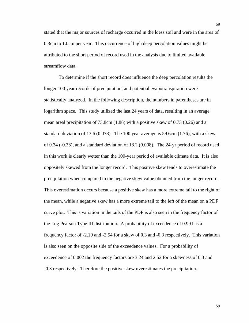
59

59

stated that the major sources of recharge occurred in the loess soil and were in the area of

0.3cm to 1.0cm per year. This occurrence of high deep percolation values might be

attributed to the short period of record used in the analysis due to limited available

streamflow data.

To determine if the short record does influence the deep percolation results the

longer 100 year records of precipitation, and potential evapotranspiration were

statistically analyzed. In the following description, the numbers in parentheses are in

logarithm space. This study utilized the last 24 years of data, resulting in an average

mean areal precipitation of 73.8cm (1.86) with a positive skew of 0.73 (0.26) and a

standard deviation of 13.6 (0.078). The 100 year average is 59.6cm (1.76), with a skew

of 0.34 (-0.33), and a standard deviation of 13.2 (0.098). The 24-yr period of record used

in this work is clearly wetter than the 100-year period of available climate data. It is also

oppositely skewed from the longer record. This positive skew tends to overestimate the

precipitation when compared to the negative skew value obtained from the longer record.

This overestimation occurs because a positive skew has a more extreme tail to the right of

the mean, while a negative skew has a more extreme tail to the left of the mean on a PDF

curve plot. This is variation in the tails of the PDF is also seen in the frequency factor of

the Log Pearson Type III distribution. A probability of exceedence of 0.99 has a

frequency factor of -2.10 and -2.54 for a skew of 0.3 and -0.3 respectively. This variation

is also seen on the opposite side of the exceedence values. For a probability of

exceedence of 0.002 the frequency factors are 3.24 and 2.52 for a skewness of 0.3 and

-0.3 respectively. Therefore the positive skew overestimates the precipitation.

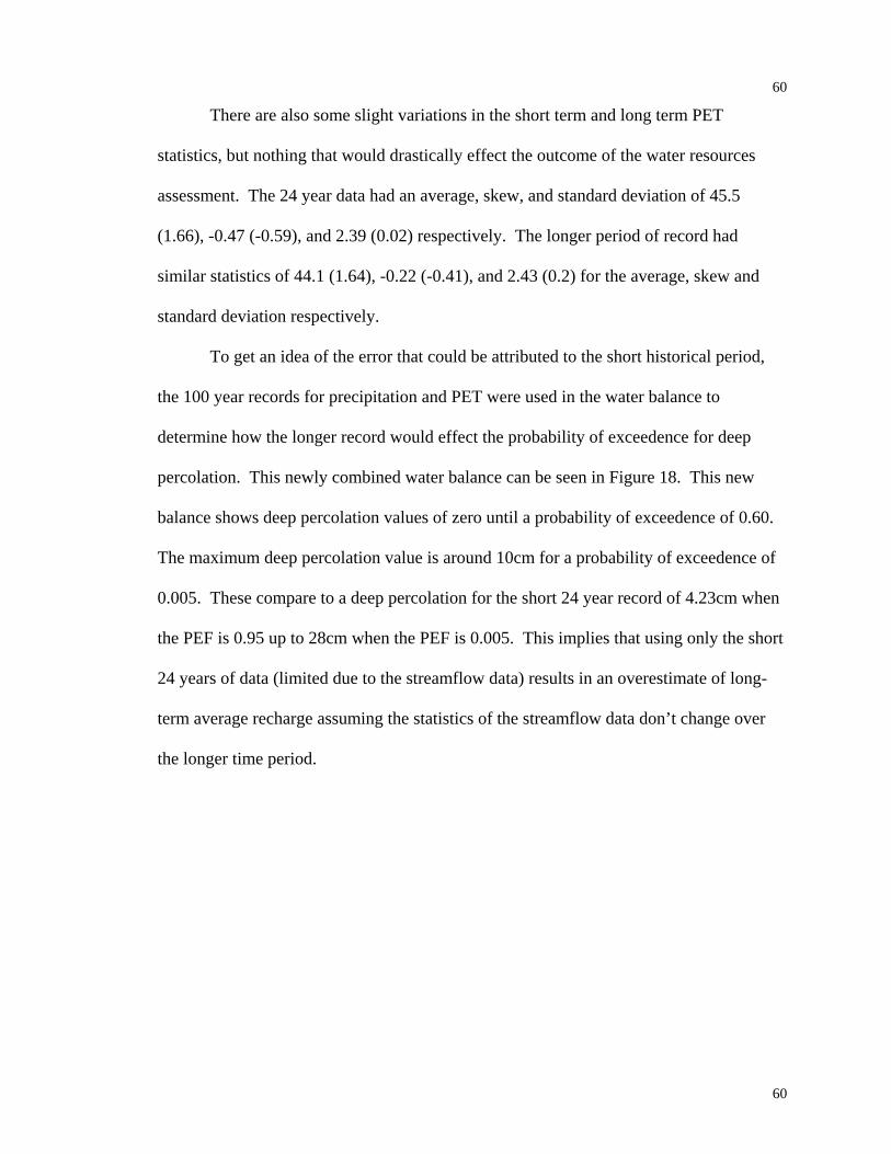
60

60

There are also some slight variations in the short term and long term PET

statistics, but nothing that would drastically effect the outcome of the water resources

assessment. The 24 year data had an average, skew, and standard deviation of 45.5

(1.66), -0.47 (-0.59), and 2.39 (0.02) respectively. The longer period of record had

similar statistics of 44.1 (1.64), -0.22 (-0.41), and 2.43 (0.2) for the average, skew and

standard deviation respectively.

To get an idea of the error that could be attributed to the short historical period,

the 100 year records for precipitation and PET were used in the water balance to

determine how the longer record would effect the probability of exceedence for deep

percolation. This newly combined water balance can be seen in Figure 18. This new

balance shows deep percolation values of zero until a probability of exceedence of 0.60.

The maximum deep percolation value is around 10cm for a probability of exceedence of

0.005. These compare to a deep percolation for the short 24 year record of 4.23cm when

the PEF is 0.95 up to 28cm when the PEF is 0.005. This implies that using only the short

24 years of data (limited due to the streamflow data) results in an overestimate of long-

term average recharge assuming the statistics of the streamflow data don’t change over

the longer time period.

61

61

0102030405060708090

100110120130


Dep

th (c

m)

PrecipitationSurface RunoffPotential ETDeep Percolation

.99 .98 .95 .9 .8 .7 .5 .3 .2 .1 .05 .02 .01 .005

Figure 18. Extended precipitation and PET record water balance probabilities of

exceedence.

Another possible source of uncertainty arises in the ability to capture and utilize

100% of the deep percolation. Historical evidence shows that when water was solely

pumped from the Wanapum aquifer that the water level dropped. This provides evidence

that 100% of the deep percolation could not be used for human consumption. This would

drastically reduce the amount of potential water available for human consumption. To

determine the change in sustainability the past five years were reevaluated using solely

surface water sources. It was assumed again that only 40% of the surface water could be

collected for human consumption. The sustainability of the Pullman-Moscow area with

the sole use of surface water sources can be seen in Table 10.

62

62

1997 1998 1999 2000 2001Precip (cm) 88.6 98.1 73.9 62.9 62.7Surface (cm) 24.6 13.9 20.7 15.7 6.8PET (cm) 44.9 47.2 46.7 45.0 46.6DP (cm) 19.1 37.0 6.5 2.3 9.3PHC (cm) 9.8 5.5 8.3 6.3 2.7AHC (cm) 20.9 21.6 22.0 22.3 22.0PHC-AHC ratio 0.47 0.26 0.38 0.28 0.12

Year

Table 10. Past 5 years PHC-AHC ratio for 40% surface water consumption.

With using only surface water for human consumption and not using any deep

percolation the past five years never would have had a sustainable system. The

possibility of collecting more surface water for human consumption exists, but even

collecting 100% of the surface water would usually result in an unsustainable system as

seen in Table 11.

1997 1998 1999 2000 2001Precip (cm) 88.6 98.1 73.9 62.9 62.7Surface (cm) 24.6 13.9 20.7 15.7 6.8PET (cm) 44.9 47.2 46.7 45.0 46.6DP (cm) 19.1 37.0 6.5 2.3 9.3PHC (cm) 24.6 17.5 20.7 15.7 6.8AHC (cm) 20.9 21.6 22.0 22.3 22.0PHC-AHC ratio 1.18 0.81 0.94 0.70 0.31

Year

Table 11. Past 5 years PHC-AHC ratio for 100% surface water consumption.

63

63

CHAPTER VI

WATER QUALITY

The use of a water resources quantity assessment in a sustainable water resources

management plan is essential. Another integral aspect of such a plan that needs

consideration is the quality of available water. General water quality issues are a concern

for Paradise Creek since it has Total Maximum Daily Load (TMDL) restrictions. More

specifically, the quality of water will determine the amount of treatment necessary to

make it acceptable for human use and consumption. This section will discuss the surface

water quality data gathered as a part of this research and relate the quality of water to the

quantity of water.

WATER QUALITY PARAMETERS

For this research the basic water quality parameters were evaluated. These

parameters include turbidity, electroconductivity, temperature, total coliforms, nitrates,

total suspended solids, total dissolved solids, pH, and phosphorus.

Turbidity is a water quality parameter that is easily measured and is a basic

indicator of overall water quality. Turbidity essentially determines the cloudiness of the

water in question. The clarity of water is tested by measuring the amount of light

scattered by a specified sample of water. The light is scattered by suspended material in

the water varying from suspended solids such as clay, silt, and a variety of microscopic

organisms that impede the passage of light through the water column. Since the amount

of suspended solids affects the turbidity of water, turbidity and total suspended solids can

64

64

often be correlated. Turbidity was measured using a continuous sampler as well as a

portable turbidity probe.

Electroconductivity (EC) measures the ability of water to conduct an electrical

current over a standard distance. Electroconductivity is measured in the units of Siemens

(S) per centimeter (the inverse of Ohms-cm). The amount and mobility of ions in the

water will affect the resulting measurements of the electroconductivity since these ions

conduct electricity when dissolved in water (Murphy, 2003). This measurement is

significantly influenced by temperature and therefore needs to be corrected to a

standardized temperature. Since electroconductivity depends on the amount of ions in

the water it is an excellent indicator of the amount of dissolved solids present. It can be

directly correlated to total dissolved solids (TDS) as seen in Equation 17, where TDS are

in units of mg/L and EC is measured in μS/cm.

ECFTDS C *= (17)

Sediment is continuously transported through streams and rivers. The main source

of sediment pollution occurs in the water column and not at the streambed level.

Therefore, sediment that affects the quality of water is either suspended in the water

column or dissolved.

Suspended sediments are defined as sediments and material that can be trapped by

a standard sized filter such as, “Whatman grade 934AH; Gelman type A/E; Millipore

type AP40; E-D Scientific Specialties grade 161; or other products that give

demonstrably equivalent results (Greenberg, 1992 pg. 2-55).” These suspended solids

play an important role in water quality. At high levels they can block the entrance of

light into the stream reducing photosynthesis, which in turn reduces the amount of

65

65

dissolved oxygen in the stream. High pendulous sediment amounts will also raise the

water temperature because these particles absorb heat from the sun, and this in turn will

reduce the amount of dissolved oxygen in the stream (Mitchell, 1992). Another problem

with high levels of suspended sediments is that they often carry adsorbed bacteria,

nutrients, metals, and pesticides (FISRWG, 1998).

The amounts of suspended sediments vary throughout a watershed both spatially

and temporally. High flow rates have an increased sediment carrying capacity, which

allows for higher concentrations of suspended solids. Soil erosion and agricultural

practices have a tremendous impact on the amount suspended sediments. Increased

impervious areas in urban regions will also tend to increase the suspended sediments

since storm water generally runs directly into the local streams, as it does in Moscow.

Decaying plants and animals can also contribute to higher concentrations of suspended

materials.

Dissolved solids are simply solids that have dissolved into the water to form a

solution (e.g. salt). Dissolved solids are capable of passing through the filters that retain

suspended sediments. Dissolved solids are a better indicator of the amount of ions in the

water. A high level of ions in the water can result in poor taste, high water hardness, or

even create a laxative effect (Murphy, 2003). In addition to the local geology, the same

issues and source areas that determine and influence the amount of suspended solids also

control the quantity of dissolved solids.

Temperature is a general water quality parameter, and it is easy to measure.

Temperature affects the metabolic rates of aquatic life forms as well as dissolved oxygen

concentrations. It also plays an important role on the activity of bacteria and toxic

66

66

chemicals in the water (Murphy, 2003). Seasonal climate variations, urban areas, riparian

vegetation, and stream flow rates affect water temperature. Wastewater treatment plants

and other industrial areas can influence the water temperature with point discharges.

The pH of water is another easy water quality parameter to measure. The pH of a

substance is defined as the molar concentration of hydrogen ions present in a negative

logarithmic form (Cech, 2003). This measurement is used to determine how acidic or

basic a substance is. Carbon dioxide concentrations in the water, the local geology, and

some air pollutants affect the pH of water.

Nitrates have become increasingly important in water quality. High nitrate levels

in water can affect many organisms dependent upon that water, especially humans.

Human congestion of high nitrate levels in water will result in reduced oxygen carrying

capacity of red blood cells. This condition is known as methemoglobinemia or "blue

baby" syndrome from the extremities turning blue from lack of oxygen. It is a concern

especially for infants since they lack the appropriate enzymes to try and correct it

(Murphy, 2003). Methemoglobinemia can also occur in other animals if nitrate levels are

high enough. A similar illness, called brown blood disease, can also infect fish that live

in waters of high nitrate concentrations (MSU, 2002). High nitrate levels stimulate plant

and algae growth, leading to eutrophication. Agricultural fertilizers, animal waste, and

WWTP effluent affect nitrate levels.

Phosphorus is another contaminant in water that arises from human activity

around streams such as agricultural fertilizers, detergents, animal waste, paved surfaces,

and WWTP effluent. These phosphates can occur in either organic or inorganic forms

depending on their origin. Extremely high levels of phosphates can lead to digestive

67

67

problems for humans (Murphy, 2003). The presence of phosphates in streams will

increase eutrophication rates and from oxygen reductions could cause fish kills.

RESULTS

These water quality parameters were measured to determine the overall quality of

water flowing in Paradise Creek. These data are important to the decision making

process regarding the use of surface water for potential drinking water use. Water

quantities versus quality relationships were derived to aid in this process as well.

Relationships between select water quality parameters were developed to allow for future

fast and economical determination of various water quality parameters.

The pH of Paradise Creek was measured at over ten locations for a period of over

two years by the IASCD and at the three University of Idaho gaging stations for a year.

These data were compared to the EPA standards for drinking water, which states that the

pH is restricted to between 6.5 and 8.5, where 7 is neutral (EPA, 2003). These data are

presented in Figure 19. There was only one seasonal occurrence per year where the pH

was out of the drinking water limits, but remained in the bounds of 6.5-8.5 for surface

water quality (Myler, 2002). This specific out of bounds occurrence usually occurred

during periods of high discharge. Increased salt loads and/or fertilizer runoff could cause

this raise in pH. These limited occurences indicate that the pH of the water is not a major

concern to users of Paradise Creek.

68

68

pH Levels

5

5.5

6

6.5

7

7.5

8

8.5

9

9.5

10

12/98 12/99 12/00 12/01 12/02

Time

pH o

f Wat

er

Figure 19. Water pH levels in Paradise Creek.

Nitrate concentrations were measured at the three University of Idaho stream

gaging locations. Nitrate levels are observed to increase through the agricultural area.

This could be related to increases in fertilizer use through the agricultural area, livestock

and/or higher erosion rates in the agricultural area. A seasonal variation of nitrate levels

is also evident, as nitrate levels tend to increase during spring melt and runoff (Figure

20). This could be caused by increased sediment loads from barren agricultural fields, or

from increased flow volumes, but no certain conclusions can be made. During the spring

2002 runoff season, nitrate levels slightly exceed the maximum contaminant level

established by the EPA of 10 mg/L.

69

69

0

2

4

6

8

10

12

14

03/19/02 05/19/02 07/19/02 09/18/02 11/18/02 01/18/03 03/20/03

Date

Nitr

ates

(mg/

L)

MWWTP Darby

Figure 20. Yearly nitrate levels for Darby and MWWTP stations.

The spatial temperature variations of Paradise Creek are in general agreement

with the River Continuum Concept. This concept states that water temperatures will

increase as the river moves from its headwaters down to its outlet (Jorde, 2003). For

example, if the water temperature at the Darby gaging site is 12oC the temperature at the

MWWTP gaging site would be expected to be 12oC or greater. There is also a strong

seasonal variation in the water temperatures with it reaching a maximum in the month of

August and a minimum temperature in January. Both of these variations can be seen in

Figure 21. These monthly values were obtained from 15 minute data that was reduced

down to monthly averages. Daily temperature variations can be found in Appendix B.

The TMDL requirements of Paradise Creek state that the water temperature should never

exceed 20 degrees Celsius, and this constraint is currently being met (IDEQ, 1997).

70

70

0.0

2.0

4.0

6.0

8.0

10.0

12.0

14.0

16.0

18.0

1 2 3 4 5 6 7 8 9 10 11 12

Month

Wat

er T

empe

ratu

re (o C

)

DarbyMWWTP

Figure 21. Yearly temperature variations for Darby and MWWTP stations.

The turbidity of Paradise Creek was continuously monitored at the University of

Idaho gaging stations. It is shown in Figure 22, that turbidity is linearly correlated to

discharge. The turbidity and discharge data were passed through a low pass four hour

moving average filter to help eliminate some variations and noise present in the raw 15

minute data.

During the year the University of Idaho gaging stations collect water samples

from the stream using the ISCO sampler. The time of these samples are recorded in the

data logger along with the continuously monitored water quality parameters. These

samples are used to measure the total suspended solids in the water. The turbidity of the

water is also tested and recorded by the data logger every 15 minutes. Combining the

TSS with the turbidity at the time the TSS water sample was taken allowed for the

determination of another useful relationship. Using the total suspended solid

measurements, a relationship was developed to determine the TSS from the turbidity.

This creates a fast efficient way of obtaining an accurate measurement of the total

71

71

suspended solids. This relationship does, however, vary from location to location.

Figure 23, shows this relationship for the MWWTP and Darby locations.

y = 2.6839x + 23.368R2 = 0.9339

0

100

200

300

400

500

600

700

0 50 100 150 200 250

Discharge (cfs)

Turb

idity

(NTU

)

Figure 22. Turbidity and discharge relationship for MWWTP.

MWWTPTSS = 1.1929Turbidity

R2 = 0.8178

DarbyTSS = 0.4322Turbidity

R2 = 0.7932

0

200

400

600

800

1000

1200

0 200 400 600 800 1000

Turbidity (NTU)

TSS

(mg/

L)

MWWTPDarby

Figure 23. Turbidity and total suspended solids relationship for Darby and MWWTP.

A linear relationship between TDS and EC was developed for Paradise Creek.

The correlation, presented in Figure 24, enables rapid computation of TDS from the

easily measured electroconductivity. The continually monitored EC at the University of

Idaho gaging stations allows the computation of daily and or annual total dissolved

72

72

solids. When combined with the daily or annual total suspended solids the total solids

can be determined. Total solids can be used to approximate the volume of sediment

carried by the stream. Total solids will be an important treatment design consideration if

surface water is used as a drinking water source in the future

TDS vs EC

TDS = 0.4978*ECR2 = 0.99

050

100150200250300350400

0 100 200 300 400 500 600 700 800

Electroconductivity (μS/cm)

Tota

l Dis

solv

ed S

olid

s (m

g/L)

Figure 24. Total Dissolved Solids and Electroconductivity in Paradise Creek.

Total coliforms were measured in samples collected at the University of Idaho

gages. The method used to measure the concentration of coliforms in the water samples

was the most probable number method. Total coliforms at all locations for every sample

obtained were greater than 1600 MPN. These high levels of coliforms are an indicator of

poor water quality. If Paradise Creek is ever utilized for drinking water, the presence of

coliforms at these levels will require the water to be treated before it is used for human

use.

Phosphates were tested by the IASCD during their sampling period of 1999-2002.

These sampling results were then compared to other more cost effective parameters to

develop a relationship for determining the concentration of phosphorus in Paradise Creek.

The best relationship derived relates phosphorus to turbidity and is given in Figure 25.

73

73

This relationship now allows for the continuous monitoring of phosphorus at the

University of Idaho stations.

y = 0.0021x + 0.0931R2 = 0.6379

00.10.20.30.40.50.60.70.80.9

1

0 25 50 75 100 125 150 175 200

Turbidity (NTU)

Tota

l Pho

spho

rus

(mg/

L)

Figure 25. Turbidity and total phosphorus in Paradise Creek.

The initial surface water quality study that was completed as part of this research

enables future planners to get a rough estimate of treatment costs if and when surface

water is used for human consumption to obtain a more sustainable water resources

system. It was shown that the general quality of water diminishes with increases in

discharge. This is true for turbidity, TSS, pH, coliforms, and phosphorus. The high

coliform counts and high sediment yields of Paradise Creek are going to make water

treatment mandatory before human consumption is possible. Other water quality

parameters and issues will have to be evaluated if surface water will be artificially

injected or infiltrated into the aquifers. These extra tests will have to determine the

treatment the water receives infiltrating down and also the hydro-geochemistry

interactions of the aquifer water with the surface water. This type of study will determine

whether surface storage or artificial injection into the aquifer is more economical for

future use.

74

74

CHAPTER VII

CONCLUSIONS

A probabilistic water resources balance for the Paradise Creek watershed was

developed. This water resources balance combined available historical data records and

common mathematical models, and thus can be applied to similar watersheds. The

probabilistic balance approach can easily be used to determine the water available for

human consumption, and be used to determine water resources sustainability. The ability

to probabilistically represent any component of the water resources balance enables

future users the ability to account for natural variations that occur in weather patterns. It

is also a more idealistic format for implementing a sustainable water resources plan since

uncertainties can be quantified.

In completing this water resources assessment, the temporal variation of the water

resources components within the watershed has been defined. Precipitation was analyzed

using a spatially distributed model, PRISM, and historical weather data from a local

weather station to create a mean areal precipitation. Precipitation was shown to increase

in a north to northwesterly direction. This spatial variation agrees with the elevation

layout of the watershed with the most precipitation occurring in the high mountainous

areas. The majority of precipitation occurs during the winter months of December

through March and is in the form of snow, rain, or a mix of both with low intensities.

From the probabilistic analysis completed on the precipitation in the watershed it was

determined that there is a 50% chance of exceeding an annual precipitation of 67cm, but

can range anywhere from 47cm to 122cm.

75

75

The quantity and timing of surface water runoff has also been defined. Surface

runoff is most evident during periods of higher precipitation and the spring snowmelt

occurring during the months of February through April. Low flow conditions during the

months of July, August, and September result in some areas of the creek in the

headwaters being completely dry. Surface runoff was analyzed using historical data from

a USGS gaging site just upstream of where the stream exits the watershed. Surface

runoff was determined to vary on an annual scale from 3.1cm to 42cm, with a 50%

chance of exceeding 13cm.

Potential evapotranspiration was determined utilizing the historical temperature

data available at the weather station. These data were converted to PET using the

Hargraeves model, which is a widely used model. The PET was corrected for the

variations in land use using an areal weighted crop coefficient. Potential

evapotranspiration was determined to vary between 39cm and 51cm, with a 50% chance

of exceeding 46cm.

Utilizing the probabilistic ditributions of the other components of the water

balance a derived distribution was used to determine the probability of deep percolation

values. This derived distribution used the inverse functions of the CDFs. Deep

percolation on an annual scale was determined to range between 3.3cm and 29cm, with a

50% chance of exceeding 8.5cm. This distribution of deep percolation was high when

compared to average deep percolation values estimated by others in the area. These high

values could be from the short historical period being used for computation.

These elements of the water balance were combined to create a probabilistic water

resources balance. This balance was used to determine the quantity of water available for

76

76

potential human consumption. This was then compared to the probability of actual

human consumption to determine if the Moscow-Pullman area can become self sufficient

in creating a sustainable water resources plan. The past five years were than evaluated

for sustainability by historical groundwater use, and alternatively utilizing surface water

for human consumption. The historical use of 100% reliance upon groundwater sources

created a possible unsustainable system 80% of the time, assuming no use of the Grande

Ronde aquifer. The utilization of surface water during the past five years would have

resulted in a sustainable system 80% of the time, with no use of the Grande Ronde

aquifer. It can be concluded from this assessment that it could be possible to create a

sustainable water resources plan for the Moscow-Pullman area by utilizing the use of

surface water for human consumption.

If it is impossible to utilize the projected deep percolation that is occurring in the

region without depleting the Wanapum aquifer the region then must rely solely on

surface water. The results of using solely surface water sources for human consumption

show that there is not enough surface water flowing out of Paradise Creek to completely

satisfy the demands of the Pullman-Moscow area. These results however, are promising

considering that by utilizing Paradise Creek and other small watersheds located

throughout the region (e.g. South Fork of the Palouse River, Palouse River) collectively

they could sufficiently supply the water demands in the Pullman-Moscow area without

further depletion of the Wanapum and Grande Ronde aquifers. The collective use of

surface waters throughout the area could then lead the Pullman-Moscow region to a

sustainable system.

77

77

Relationships between the quantity and quality of surface water have also been

developed, to aide future decision makers in determining the best times to collect surface

water, and also enabling them to cost effectively monitor water quality. The measured

turbidity of the water can now be used to determine the total suspended solids, and

phosphorus content. The electroconductivity can be used to determine the total dissolved

solids in the water. Nitrates and the pH of the water tended to increase during spring

runoff and high surface flows. Basic water quality was shown to diminish as higher

water flows occurred. The high concentration of coliforms and high sediment yield of

Paradise Creek create the need to treat the surface water before it can be used for human

consumption.

RECOMMENDATIONS ON SUSTAINABILITY

The probabilistic water resources assessment on Paradise Creek watershed that

was completed for this research can lead to the implementation of a sustainable water

resources plan. The ability to probabilistically define these water resources terms and

quantify the current situation will allow future planners to determine the appropriate steps

towards sustainability and possible alternatives to the aquifer mining that is currently

taking place. This will not only secure current drinking water supplies, but will also

ensure water for future generations hundreds of years down the road. The sooner a

sustainable water resources plan is implemented into this region the safer the future will

be.

FUTURE RESEARCH

There is an almost unlimited amount of additional research that could be

conducted to improve the current probabilistic water resources assessment for the

78

78

Paradise Creek Watershed. As more data becomes available the results of this research

can be updated. With advances in computer use and technology better models will

become available for use. A further in depth study of conservation methods and their

effectiveness in the Moscow area would also improve estimates of the minimal human

consumption possible.

This section will be broken up into two parts. The first part will deal with basic

future research, while the second part will deal solely with conservation methods. This

second part consists of a literature review of available resources for conservation methods

and leads into its applicability into a sustainable water resources management plan.

General Research

When planning for the future, looking from the past to the present and applying

these trends is often the best indicator of how things will be in the future. The need to

obtain more historical data will always be of great importance. For the watershed studied

there was over 100 years of weather data available. The 24 years of discharge

measurements for Paradise Creek were the limiting factor of this probabilistic water

resource assessment. It could be possible to deterministically create discharge

measurements for the past 100 years, greatly increasing the amount of data available for

use in this type of assessment and hopefully increasing the accuracy of the probability of

exceedence values. This problem was evident in this study and was discussed in further

detail in Chapter V.

As research continues and more information becomes available on the properties

of the Grande Ronde and Wanapum aquifers (such as groundwater basin extent and

79

79

subsurface inflows/outflows), these data can be used to fill in the gaps created by the

assumptions and uncertainties in this assessment. This area is usually the last major

unknown realm in water resources assessment and it will greatly increase the confidence

in the presented results if the assumptions made could be verified. If the assumptions are

violated then the water resources assessment would need to be re-interpreted according to

the new information.

Increased studies of soil characteristics in and around the watershed area will

enable future researchers to incorporate soil moisture variations within the water

resources assessment. This will allow monthly time steps to be considered. By reducing

the time step it will be possible to see the effects of possible surface water collection on

local soils, and determine how this will effect agricultural areas and the dry land farming

techniques currently being practiced.

A new tool available in some areas is the use of satellite imagery to aid in the

determination of evapotranspiration. Spatially distributed computer models are becoming

increasingly common for evapotranspiration estimates. There are currently numerous

models available for these types of calculations. As studies continue on the effectiveness

of these methods to accurately predict evapotranspiration their application throughout the

world will only increase. There are some studies that have already been completed to

compare satellite imagery ET versus measured, and calculated ET values.

One study conducted by Granger (2000) compared measured ET versus the ET

derived from two satellite imagery systems, NOAA-AVHRR and LANDSAT. Both of

these satellites used the feedback method to calculate ET. The ET calculated from these

two methods varied from the measured ET values anywhere from 0.3-0.6 mm/day

80

80

(Granger, 2000). This type of precision greatly increases the confidence placed in ET

values for water balance equations.

Another study completed by Mauser (1998) compared ET measurements using

NOAA-AVHRR and LANDSAT imagery to measured ET. Mauser (1998) concluded

that at the current time these satellites were not capable of the appropriate spatial

resolution to obtain accurate measurements. However, within the next decade new

sensors with the ability to obtain regular measurements with increased spatial and

temporal resolution will be made available(Mauser, 1998). This will increase the

model’s ability to represent ET, and make it a more common practice for everyday users.

Morse (2000) in his final report on the application of the Surface Energy Balance

Algorithm for Land (SEBAL) methodology to estimate consumptive land use in the Bear

River Basin of Idaho displays the effectiveness to calculate ET through the use of remote

sensing data. This method incorporates the use of LANDSAT with a digital elevation

model to calculate ET. These measurements were compared to lysimeter measurements

made throughout the study area. Final results showed a relatively poor estimation of ET

with an average error of around 26%. This could be caused by possible lysimeter

measuring errors as well as pixel errors within SEBAL (Morse, 2000). The benefits of

the SEBAL model are the low data requirements, and sole reliability of satellite

information. The model is also not solely restricted to irrigated areas, but can be used

over a range of various vegetation types (Kite, 2000).

The benefits of satellite imagery for ET estimates are the high spatial resolution

along with the spatial coverage available. The main disadvantage to this method is that it

only allows for instantaneous estimates of ET (Kite, 2000). As relationships get

81

81

developed and the gaps of data between the instantaneous estimates can be filled this

method of estimating ET through the use of satellite imagery will increase in accuracy

and become more popular.

Conservation Research

The most basic method of trying to help create a more sustainable system is

conservation of the resource in peril. The conservation of water resources will allow less

water to be used overall, increasing the sustainability by a certain percent. Simple

conservation techniques could completely eliminate the depletion of water resources

within a system, if they are used on a big enough scale. Household conservation methods

to city or state regulated methods can all help alleviate the stress being applied on water

supplies.

Canada and the US use the most water in the world on a per capita basis. These

two countries on average use 1700 cubic meters per person per year. The next highest

water users are the Pacific Islands, Australia, New Zealand, Papua New Guinea, and Fiji,

which use 900 m3. Other major water consumers are Europe at 725, Asia with 525,

South America with 375, and Africa a mere 250 cubic meters per person per year.

Except for the US and Canada, these values fall below Malin Falkenmark’s mark of 1700

cubic meters per person per year as the cutoff between a nation being comfortable or

stressed for water (De Villiers, 2000). In 2000, Moscow, Idaho was using just over 0.5

cubic meters per person per day (MCPD) or 210 cubic meters per person per year

(PBAC, 2002). This is comparable to the state of Georgia, where on the average people

use 0.75 MCPD (Wade, 2003). Even with numbers well below Falkenmark’s established

limit the world and Moscow are still searching for more water.

82

82

There are many methods available to reduce the amount of water consumed daily.

To try and put a cap on daily water use Gleick (1998) recommended a “human

entitlement” of 50 liters of water per person per day. “Drinking water, 5 liters; sanitation

water, 20 liters; bathing water, 15 liters; food preparation, 10 liters. Total, 50 liters

(Gleick, 1998).” However, not even the poorest of countries uses such a small amount of

water. Not because it is impossible, nor because the technology isn’t available, but

because there is a lack of political organization (De Villiers, 2000). Moscow uses over

ten times the proposed “human entitlement” of 50 liters per day, this does however

include other uses than described by Gleick. Gleick (1998) also put into thought that a

“lifeline rate” should be used on water usage. This would mean numerous water meters

per household, but would cut down water usage significantly. This rate would charge

individuals a certain price depending on what the water was used for. For example,

watering a yard would cost much more than food preparation water (Gleick, 1998).

Hitting people in their wallet would make them more conscience of how, and when they

use their water. This would then bring into play more household conservation

techniques.

City, counties, or states could also apply water regulations to the citizens for

water conservation. Some of these ideas discussed by Gleick could be used, but currently

more moderate, less severe methods have been applied. Many cities will supply free

devices (e.g. air bricks in toilet reservoirs) to help conserve water. Some cities during

drought seasons only allow lawn watering every other day, two days per week, or only by

hand. Most of the current regulations that get activated during these hard water times

have to deal with trying to control frivolous water use. It is obvious that stricter

83

83

regulations are going need to be implemented into daily use to ensure sufficient water for

future demands.

On a household level there are many conservation methods that can be applied

daily to help save water. The problem with household methods compared to city or

county sanctioned conservation methods is that one household will not make a significant

difference, whereas an entire city will make a noticeable contribution to conservation.

The main area a household can improve in water conservation is landscaping. In the

1980’s over half of the water consumed by households went towards landscaping

(Williams, 2003). One conservation method a household can use to limit the amount of

outside watering is xeriscaping. The cities of Moscow, Pullman, and the two local

colleges are currently trying to implement this method to their lands. The term xeriscape

was introduced in 1981 by the Denver Water Department to associate water conservation

to landscape design, and allow the public to become more familiar with these types of

conservation efforts (DWD, 2003).

Xeriscaping is an old landscaping and gardening technique that is starting to come

back. People often xeriscaped in arid lands and prairies, simply because it made sense

not to waste water. There was just never a term for the method of landscaping until

recently. Xeriscaping is a seven-part process that focuses on planning and design, soil

improvement, efficient irrigation, zoning of plants, mulches, turf alternatives, and

appropriate maintenance. Step one, planning and design, deals with the basic outlay

options for vegetation on the property, and separates the property into high, medium, and

low water demand zones. Soil improvement is accomplished from analyzing the soil and

determining what nutrients and actions should be taken to make it more productive.

84

84

Efficient irrigation deals with the watering methods from automatic sprinklers for turf

areas, to drip irrigation for low water use areas. The zoning of plants deals with the

topography of the land, having high water use vegetation in the low areas where natural

runoff will go, and low water use plants in high or secluded terrain, where water will

vanish rather quickly. It also deals with selecting a type of plant that will be able to adapt

to the surroundings it will be placed in. Mulches are used to aid the soil in retaining

water moisture, because they help limit evaporative losses through the soil surface. This

increased moisture content can clearly be seen in Figure 26. Step six, deals with the

establishing the proper type of turf for use. Many types of turf are very drought resistant,

and require very little water. To keep anything in good condition proper maintenance is a

necessity. This step deals with appropriate applications of fertilizer and water, as well as

proper pruning, and mowing techniques. Through these seven steps to landscape

conservation it is probable that outdoor water usage could be reduced by fifty percent

(Wade, 2003). At the end of this section there is a list of available references for more

information on xeriscaping.

Figure 26. Water Content between bare soil and mulch covered soil (Wade, 2003).

There are many water conservation groups throughout the nation. They are all

offering methods and advice to reduce water use in households. Moscow, Idaho has a

85

85

local water conservation group called the Palouse Water Conservation Network (PWCN)

that is trying to educate the public about conservation methods available to help limit

each household’s daily water usage. Through the conservation methods they describe on

their web site and on the American Water Works Association’s (AWWA) web site a

person has the ability to seriously reduce their conjunctive water use. One local family of

four has reduced their water use to around 50 liters per day for two months (PWCN,

2003). This is over ten times less than the per capita average for Moscow of 0.5 m3. If

every person cut their water use to 0.20 MCPD, more than three times what one local

family was consuming, it would theoretically triple the current unknown life span of the

aquifers being mined. Table 10, depicts allocated water usage for a normal and a

conservation-oriented household showing the savings that could theoretically occur. It

does not take into account any outdoor water use.

Without Conservation With Conservation Savings

End Use Share gpd Share gpd % gpd Toilets 27.70% 20.1 19.30% 9.6 52% 10.5 Clothes Washers

20.90% 15.1 21.40% 10.6 30% 4.5

Showers 17.30% 12.6 20.10% 10 21% 2.6 Faucets 15.30% 11.1 21.90% 10.8 2% 0.3 Leaks 13.80% 10 10.10% 5 50% 5 Other Domestic

2.10% 1.5 3.10% 1.5 0% 0

Baths 1.60% 1.2 2.40% 1.2 0% 0 Dish Washers

1.30% 1 2.00% 1 0% 0

Inside Total

100% 72.5 100% 49.6 32% 22.9

Table 12. Household use of water with and without conservation (AWWA, 2003).

There are many methods and techniques to water conservation. One of the major

sources of wasted water is leaky pipes, fixtures, and appliances. This water is lost in the

system, yet from a study done by the AWWA (2003) 38 liters per day are lost through

86

86

leaks alone. Another major consumer of water in a household is the toilet. They roughly

represent 30% of the indoor water use in a household. By converting from an old

standard toilet to a low flow flush toilet it could be saving anywhere from 7.5 to 20 liters

per flush, or on average 40 liters per day (AWWA, 2003). If a quick shower with a low

flow showerhead is taken instead of a bath a person can save 75 liters of water. If all the

leaks were fixed, an ultra low flow toilet, and a low flow showerhead were installed a

person could be saving as much as 0.15 MCPD. Other indoor conservation tips include:

turning the faucet off while shaving or brushing teeth, running the dishwasher, and

washer only when there is a full load, cleaning fruits and vegetables in a sink of water

rather than running water, and rinsing dishes in a sink of water instead of running water.

Cutting the amount of water used outside the house will also decrease the daily

consumption a person uses. A house with an in ground sprinkler system will use 37%

more water for irrigation than a house without an in ground sprinkler system. Watering a

yard by hand is 30% more efficient on water use than using a sprinkler (AWWA, 2003).

One technique to save water is washing a car with a bucket of water, instead of using a

running hose. Other methods include: cleaning sidewalks with a broom instead of water,

water a yard only when it starts to be stressed, water it in early morning or late evening to

lower the amount of evaporation that could occur, and covering pools and spas to help

eliminate unnecessary evaporation. Landscaping using the xeriscape method described

above will also greatly reduce the amount of water consumed outdoors.

Per capita water conservation throughout households can greatly reduce the

amount of water consumed on a daily and annual basis and help establish a more

sustainable water resources system. Through xeriscaping, and proper indoor and outdoor

87

87

conservation techniques people should be able to drastically reduce the amount of water

being wasted. This is an easy first step towards achieving the ultimate goal of a

sustainable water resources system throughout the Palouse area.

For future studies it will become increasingly important to use the latest

technologies available. Through the use of satellite imagery, to better represent

evapotranspiration and the incorporation of major water conservation efforts into the

water resources assessment these factors will help lead to a more accurate water

resources assessment to create a better sustainable system in the Palouse Basin.

88

88

REFRENCES

Allen, R.G., Pereira, S., Raes, D., Smith, M., 1998. FAO irrigation and drainage paper no. 56 crop evapotranspiration (guidelines for computing crop water requirements).

Anderson, M.T., Woosley, L.H. Jr, 2002. Science to support the management of western water, The Geological Societies of America Conference, Denver, CO.

ASCE, 1998. Sustainability criteria for water resource systems. Division of Water Resource Planning and Management. American Society of Civil Engineers, Reston, VA.

AWWA, 2003. American Water Works Association. AWWA.

Baines, C.A., 1992. Determination of sustained yield for the shallow basalt aquifer in the Moscow area, Idaho Water Resources Research Institute.

Barker, R.J., 1981. Soil survey of Latah county area Idaho. USDA SCS, Washington D.C.

Bauer, H.H., Vaccaro, J.J., 1990. Estimates of groundwater recharge to the Columbia Plateau regional aquifer system, Washington, Oregon, and Idaho, for predevelopment and current land-use conditions: USGS Water Resources Investigations Report 88-4108, USGS.

Benson, M.A., 1968. Uniform flood-frequency estimating methods for federal agencies. Water Resources Research, 4(5): 891-908.

Biftu, G.F., Gan, T.Y., 2000. Assessment of evapotranspiration models applied to a watershed of Canadian prairies with mixed land-uses. Hydrological Processes, 14: 1305-1325.

Biswas, A.K., 1994. Sustainable water resources development: some personal thoughts. Water Resources Development, 10(2): 109-116.

Bloomsburg, G.L., 1959. A water balance study of two small watersheds, University of Idaho, Moscow, 66 pp.

Boll, J., 2003. Paradise Creek: an education and research watershed.

Brooks, E.S., McDaniel, P.A., Boll, J., 2000. Hydrologic modelling in watersheds of the eastern Palouse: estimation of subsurface flow contributions, Pacific Northwest ASAE Regional Meeting. ASAE, St. Joseph, MI.

Brooks, J., 1992. The concepts of sustainable development and environmentally sound technology. ATAS Bulletin, 7: 19-24.

89

89

Cech, T.V., 2003. Principles of water resources; history, development, management and policy. John Wiley & Sons, Inc., New York, NY.

Cherry, J.G., 1986. A water balance and hydrologic analysis of Crumarine creek watershed, University of Idaho, Moscow, 120 pp.

Chow, V.T., Maidment, D.R., Mays, L.W., 1988. Applied Hydrology. McGraw-Hill series in water resources and environmental engineering. McGraw-Hill Inc., US.

Cook, M.R., 2002. Water resource comprehensive plan outline, City of Moscow, Moscow, ID.

Davis, D.J., 1971. A water balance on a small agricultural watershed, Latah county, Idaho, University of Idaho, Moscow, 88 pp.

De Villiers, M., 2000. Water the fate of our most precious resource. Houghton Mifflin Company, New York, pp. 352.

De Vries, J.J., Selaolo, E.T., Beekman, H.E., 2000. Groundwater recharge in the Kalahari, with reference to paleo-hydrologic conditions. Journal of Hydrology, 238(1): 110-123.

Dingman, S.L., 2002. Physical Hydrology. Prentice Hall, Upper Saddle River, NJ.

DWD, 2003. Xeriscape information. Denver Water Department.

EPA, 2003. Groundwater and drinking water.

FISRWG, 1998. Stream Corridor Restoration: principles, processes, and practices. Federal Interagency Stream Restoration Wroking Group.

Gleick, P.H., 1998. Water in crisis: paths to sustainable water use. Ecological Applications, 8(3): 571-579.

Goodwin, R.B., Foxworthy, B.L., Vladimirov, V.A., 1990. Guidelines for water resources assessments of river basins, UNESCO, Paris.

Granger, R.J., 2000. Satellite-derived estimates of evapotranspiration in the Gediz basin. Journal of Hydrology, 229: 70-76.

Greenberg, A.E., Clescerl, L.S., Eaton, A.D. (Editor), 1992. Standard methods for the examination of water and wastewater. APHA, AWWA, WEF, Washington DC.

Hargraeves, G.H., and Z.A. Samani, 1982. Estimating potential evapotranspiration. ASCE Journal of Irrigation and Drainage Division, 108(3): 225-230.

Hillel, D., 1982. Introduction to soil physics. Academic Press, New York, NY.

90

90

IDEQ, 1997. Paradise Creek TMDL: water body assessment and total maximum daily load, Idaho Department of Environmental Quality.

Jorde, K., 2003. CE 504 Habitat Quality Modeling. In: J.J. Fealko (Editor), Moscow, ID.

Kite, G.W., Droogers, P., 2000. Comparing evapotranspiration estimates from satellites, hydrological models and field data. Journal of Hydrology, 229: 3-18.

Kulshreshtha, S.N., 1993. World water resources and regional vulnerability: impact of future changes. IIASA, Luxemburg.

Kundzewicz, Z.W., 1997. Water resources for sustainable development. Journal of Hydrological Sciences, 42(4): 467-480.

Kundzewicz, Z.W., 2001. Some for all, forever - sustainable development and management of water resources. International Journal of Sustainable Development of World Ecology, 8: 290-298.

Larsen, T.A., Gujer, W., 1997. The concept of sustainable urban water management. Water Science Technology, 35(9): 3-10.

Larson, K.R., Keller, C.K., Larson, P.B., Allen-King, R., 2000. Stable isotope evidence for low recharge rate to a confined basalt aquifer: Implications for water resource development, Moscow.

Loucks, D.P., 2000a. Sustainable water resources management. Water International, 25(1): 3-10.

Loucks, D.P., Stakhiv, E. Z., Martin, L. R., 2000b. Sustainable Water Resources Management Editorial. Journal of Water Resources Planning and Management: 43-47.

Lum, W.E.I., Smoot, J.L., Ralston, D.R., 1990. Geohydrology and numerical model analysis of ground-water flow in the Pullman-Moscow area, Washington and Idaho: USGS Water Resources Investigations Report 89-4103, USGS.

Marsily, G.d., 1986. Quantitative hydrogeology: groundwater hydrology for engineers. Academic Press, San Diego, CA.

Mauser, W., Schadlich, S., 1998. Modelling the spatial distribution of evapotranspiration on different scales using remote sensing data. Journal of Hydrology, 212-213: 250-267.

McCuen, R.H., 1998. Hydrologic Analysis and Design. Prentice Hall, Upper Saddle River, NJ.

McKenna, J.M., 1999. The palouse basin aquifer committee 1999 annual report, PBAC, Moscow, ID.

91

91

Miloradov, R.M., Marjanovic, P., Cukic, Z., 1995. Water resources assessment as the basic tool for sustainable and environmentally sound river basin management. Water Science Technology, 32(5-6): 45-53.

Mitchell, S., 1992. Field manual for water quality monitoring.

Mohan, S., 1991. Intercomparison of evapotranspiration estimates. Hydrological Sciences Journal, 36(5): 447-461.

Monteith, J.L., 1965. Evaporation and the environment. Symposium Soc. Expl. Biol., 19: 205-234.

Morse, A., Tasumi, M., Allen, R.G., Kramber, W.J., 2000. Application of the SEBAL methodology for estimating consumptive use of water and streamflow depletion in the bear river basin of idaho through remote sensing, Idaho Department of Water Resources.

MSU, 2002. Information sheet 1390. MSU.

Murphy, S., 2003. Information on water quality parameters. city of Boulder/USGS.

Murray, J.G., 2002. Development of a GIS database for recharge assessment of the palouse basin, University of Idaho, Moscow, ID, 82 pp.

Myler, C., 2002. Paradise Creek Monitoring Report 2002, Idaho Association of Soil Conservation Districts, Moscow.

O'Brien, R.O., Keller, C.K., Smith, J.L., 1996. Multiple tracers of shallow ground-water flow and recharge in hilly loess. Ground Water, 34(4): 675-682.

O'Green, A.T., 2002. Assessment of hydrologic processes across multiple scales in soil/paleosol sequences using environmental tracers, University of Idaho, Moscow, ID, 116 pp.

PBAC, 2002. Palouse Basin Aquifer Committee. PBAC.

Plate, E.J., 1993. Sustainable development of water resources: a challenge to science and engineering. Water International, 18: 84-94.

PWCN, 2003. Palouse Water Conservation Network. PWCN.

Rangarajan, R., Athavale, R.N., 2000. Annual replenishable ground water potential of India-an estimate based on injected tritium studies. Journal of Hydrology, 234(1): 38-53.

Reisner, M., 1993. Cadillac Desert the american west and its disappearing water. Penguin, New York, 582 pp.

Russel, I.C., 1897. A reconnaissance in South-Eastern Washington: USGS Water Supply Paper 4, USGS.

92

92

Saeed, M., 1986. The estimation of evapotranspiration by some equations under hot and arid conditions. Transactions of the American Society of Agricultural Engineers, 29(2): 434-438.

Sakiyan, J.H.Y., 2002. Comparison of safe and sustainable yields: a case study of an overexploited aquifer in western turkey, The Geological Societies of America Conference, Denver, CO.

Simmers, I.E., 1987. Estimation of natural groundwater recharge. R. Reidel Publishing Company, Netherlands.

Simonovic, S.P., 1997. Risk in sustainable water resources management. In: D.B. Rosbjerg, NE; Gustard, A; Kundzewicz, Z.W.; Rasmussen, P.F. (Editor), Fifth Scientific Assembly of the International Association of Hydrological Sciences. IAHS, Rabat, Morocco, pp. 3-17.

Smoot, J.L., 1987. Hydrogeology and mathematical model of ground-water flow in the Pullman-Moscow region, Washington and Idaho, University of Idaho, Moscow, ID, 118 pp.

Sophocleous, M., 2000. From safe yield to sustainable development of water resources-the kansas experience. Journal of Hydrology, 235: 27-43.

Stevens, Thompson, Runyan, 1970. Water supply study for the Pullman-Moscow water resources committee, Moscow.

Stillman, S.T., Wilson, J.P., Daly, C., Hutchinson, M.F., Thornton, P.E., 2003. Comparison of ANSUPLIN, MTCLIM-3D, and PRISM precipitation estimates, University of Montana, Missoula, MT.

Tabios III, G.Q.S., Jose D., 1985. A comparative analysis of techniques for spatial interpolation of precipitation. Water Resources Bulletin, 21(3): 365-380.

USCB, 2003. World population information. US Census Bureau.

Wade, G.L., Midcap, J.T., Coder, K.D., Landry, G., Tyson, A.W., Weatherly, N.Jr, 2003. Xeriscape: a guide to developing a water wise lanscape. University of Georgia.

WCED, 1987. Our common future ("The Brundtland report"). Oxford University Press, Oxford, U.K.

Williams, S., 2003. Xeriscape landscaping.

WRC, 1982. Guidelines for determining flood flow frequency. Bulletin, N. 17B of thge Hydrology Committee, Washington D.C.

93

93

Wu, I.-P., 1997. A simple evapotranspiration model for Hawaii: the Hargraeves model. College of Tropical Agricultural & Human Resources, University of Hawaii at Manoa, Engineer's Notebook, 106.

fealko thesis water resources - University of Idaho · For surface water collection purposes a...

Documents

Transcript of fealko thesis water resources - University of Idaho · For surface water collection purposes a...