FEA Information Engineering Journal - FEAIEJ Information Engineering Journal March... · FEA...

ISSN 2167-1273 Volume 3, Issue 3, March 2014

FEA Information Engineering Journal

DYNAmore Nordic AB Publications


Aim and Scope FEA Information Engineering Journal (FEAIEJ™) is a monthly published online journal to cover the latest Finite Element Analysis Technologies. The journal aims to cover previous noteworthy published papers and original papers. All published papers are peer reviewed in the respective FEA engineering fields. Consideration is given to all aspects of technically excellent written information without limitation on length. All submissions must follow guidelines for publishing a paper, or periodical. If a paper has been previously published, FEAIEJ requires written permission to reprint, with the proper acknowledgement give to the publisher of the published work. Reproduction in whole, or part, without the express written permissio of FEA Information Engineering Journal, or the owner of of the copyright work, is strictly prohibited. FEAIJ welcomes unsolicited topics, ideas, and articles. Monthly publication is limited to no more then five papers, either reprint, or original. Papers will be archived on www.feaiej.com For information on publishing a paper original or reprint contact [email protected] Subject line: Journal Publication

Cover: Drilling rotation constraint for shell elements in implicit and explicit analyses Figure 7: Deformed crashrail with DRCPRM=0.01 (left), 1.0 (middle), and 100.0 (right)

2 Fea Information Engineering Journal March 2014

http://www.feaiej.com/

mailto:[email protected]


TABLE OF CONTENTS

Publications are © to LS-DYNA 2013 9th European Users‘ Conference

A General Damage Initiation and Evolution Model (DIEM) in LS-DYNA Thomas Borrvall, Thomas Johansson and Mikael Schill, DYNAmore Nordic AB Johan Jergéus, Volvo Car Corporation Kjell Mattiasson, Volvo Car Corporation and Chalmers University of Technology Paul DuBois, Consulting Engineer

Drilling rotation constraint for shell elements in implicit and explicit analyses

Tobias Erhart, Dynamore GmbH, Stuttgart, Germany Thomas Borrvall Dynamore Nordic AB, Linköping, Sweden

A Quadratic Pipe Element in LS-DYNA®

Tobias Olsson, Daniel Hilding DYNAmore Nordic AB

All contents are copyright © to the publishing company, author or respective company. All rights reserved.

3 Fea Information Engineering Journal March 2014

© 2013 Copyright by Arup

A General Damage Initiation and Evolution Model (DIEM) in LS-DYNA

Thomas Borrvall, Thomas Johansson and Mikael Schill, DYNAmore Nordic AB

Johan Jergéus, Volvo Car Corporation

Kjell Mattiasson, Volvo Car Corporation and Chalmers University of Technology

Paul DuBois, Consulting Engineer

1 Introduction

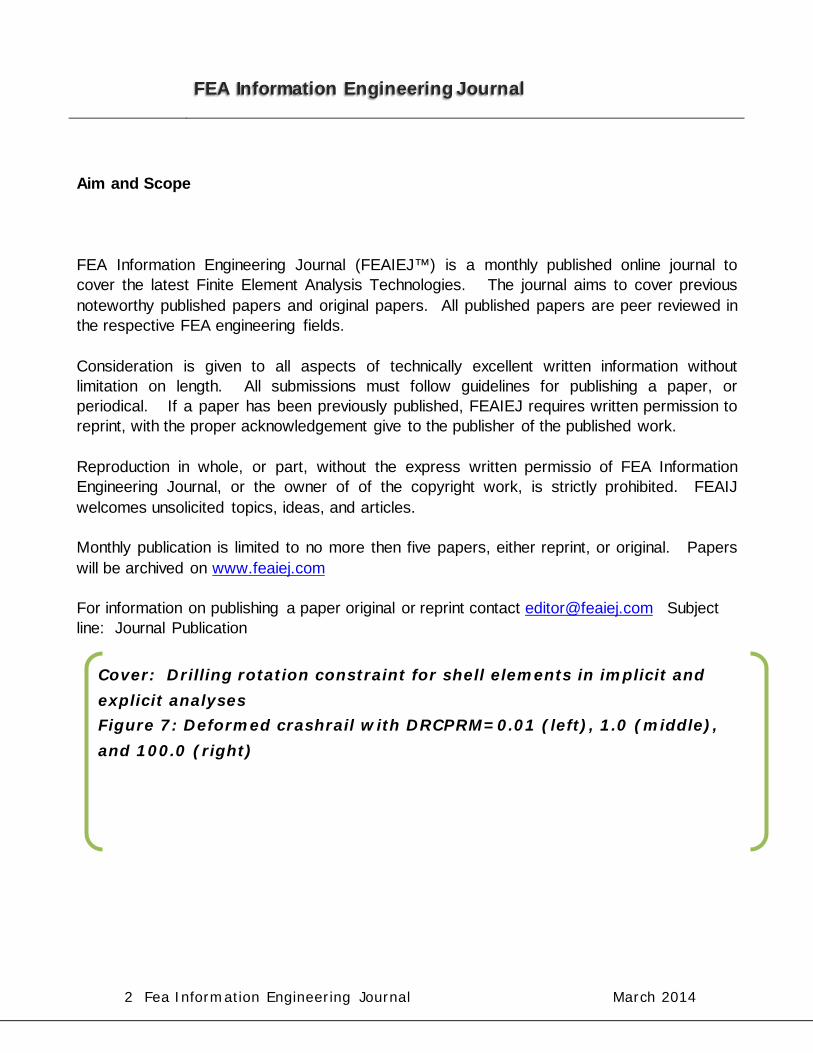
As the automotive industry is reducing the number of physical prototypes in favour of computer simulations during their design processes, a lot of demands is put on the accuracy of the virtual finite element models used for this purpose. In this context the mathematical modelling of fracture is of major importance and has been a field of intense research over the past 50 some years. There are numerous fracture models implemented in LS-DYNA, but as of tradition a fracture model is statically linked to the underlying constitutive model which in practice limits its usage to a single stage of the design process. Recently GISSMO [1,2,3] was introduced in an attempt to remedy this shortcoming by allowing the fracture model to be separated from the constitutive model, thus facilitating results from manufacturing simulations to be transferred to subsequent crash simulations. Behind GISSMO, the Damage Initiation and Evolution Model (DIEM) was developed in the same spirit and with similar capabilities, but this model has to the authors’ knowledge not been used extensively. The intention with this paper is to present this latter fracture model and compare it with GISSMO and, to some extent, with CrachFEM [4] to which it has superficial similarities. Fig 1 Illustration of an FLD diagram and fracture along linear and nonlinear strain paths.

2 Fracture modelling

2.1 Plastic instability and the FLD diagram

Failure in sheet metals are either due to material instability with localized deformation or fracture from initiation, growth and coalescence of voids, or a combination of the two. The onset of material instabilities depends to a great extent on the material properties including yield strength, strain hardening and rate dependency as well as geometry imperfections of the sheet. Usually plastic

εmin

εmaj

9th European LS-DYNA Conference 2013 _________________________________________________________________________________


instability with localized necking takes place before any other failure mechanism, and can either be mathematically predicted using for instance the Marciniak-Kuczynski method [5] or established through material tests. In either case, a common representation of the instability characteristics of a metal sheet is through a Forming Limit Curve (FLC) in a Forming Limit Diagram (FLD), as illustrated in Fig 1. The FLC is a function of the minor in-plane principal (plastic) strain

)( min*maj

*maj εεε =

and gives the points where instability occurs in the in-plane principal strain space. The safe zone is given by the inequality

*majmaj εε < ,

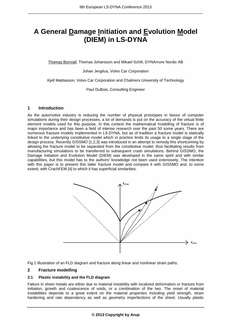
i.e., the area below the FLC curve, and the strains should typically reside in this region. The FLC curve is usually restricted to linear strain paths, i.e., straight lines in the FLD diagram, and for nonlinear paths instability may occur either below or above the FLC curve as illustrated in Fig 1. Fig 2 FLC curve represented as critical plastic strain versus triaxiality.

With the restriction to linear strain paths and von Mises associative plasticity, the FLC can be equivalently represented in terms of critical effective plastic strain as function of either triaxiality defined as the ratio of mean stress over von Mises equivalent stress,

q

p−=η ,

or principal in-plane deviatoric stress ratio,

maj

min

s

s=α ,

whatever most convenient. An example of this representation is shown in Fig 2 together with a linear strain path to failure represented by the vertical arrow and nonlinear strain paths represented by the curved arrows. The dashed lines indicate the linear strain paths corresponding to uniaxial compression, shear, uniaxial tension and biaxial tension, and Table 1 lists common stress states and associated triaxiality and deviatoric stress ratio values.

η

εp

2/3 1/3 -1/3



Table 1 Triaxiality and deviatoric stress ratio for some common stress states.

Load case η α Biaxial tension 2/3 1 Plane strain tension 1/√3 0 Uniaxial tension 1/3 -1/2 Shear 0 -1 Uniaxial compression -1/3 -2 Plane strain compression -1/√3 -∞ Biaxial compression -2/3 1

The effective plastic strain evolves with the principal components of the plastic strain rate tensor as

majmin2maj

2min

3

2 εεεεε &&&&& ++=p

and the safe zone is for plastic strains smaller than the critical plastic strain,

pD

p εε < , i.e., the area under the FLC represented in Fig 2. Obviously nonlinear strain paths is a concern, and one way to account for this is to introduce an instability indicator

0≥Dω that somehow evolves with plastic strain and depends on the stress state, i.e.,

0),(),( ≥== αεωηεωω pD

pDD &&&&& ,

and instability is said to occur when

1=Dω . This instability model has to be accompanied with the restriction that it reconciles with the FLC representation for linear strain paths, which mathematically can be expressed as

10

=∫pD

ppD d

ε

εεω&

& for constant η or α.

This suggests the following obvious evolution law,

pD

p

D εεω&

& = , (1)

although there is freedom to choose any other within reason.

2.2 Post-instability and damage modelling

Independent of the model of choice to predict instability, there is the delicate matter of what happens after instability has occurred, i.e., the post-instability stage. To this end it is important to note that the reason for having an instability model in the first place is that the actual material instability phenomenon cannot be captured in the finite element model itself due to coarseness of the numerical discretization. This means that numerical results are in effect only reliable up to the instability point, and to model what really happens after that and up to the point of fracture borders to the art of



guesswork. The simplest way out would be to reconcile a fracture model with the assumption that fracture in practice occurs very soon after instability onset and whence simply erode the material when instability has been detected. If this approach leads to results that are inconsistent with the real-life behaviour then one may need to actually model the post-instability stage. A damage model can be seen as a homogenization model of the micromechanical composition of material and void that accordingly augments the stress from the constitutive model for the formation of internal forces. A simple phenomenological approach is taken by introducing a damage parameter, 10 <≤ D , that is assumed to reduce the effective cross-sectional area in the direction of loading. This is to say that the homogenized stress, i.e., the stress used to model the global response, can be expressed in terms of the stress used in the constitutive law as σσ

~)1( D−= , (2)

i.e., the material is isotropically degraded with damage. This is the Continuum Damage Mechanics concept and was introduced by Lemaitre [6]. The physical interpretation of this model is usually that the area is reduced due to the formation of cavities that develop in the material during plastic loading, i.e., the material is damaged in the true sense of the word, but other interpretations may apply in the event that it just serves as a means to model, or induce, the post-instability response of the material. As the instability parameter, the damage parameter is assumed to evolve with plastic strain and depend on the stress state, but in this case we introduce two further dependencies for the following reasons.

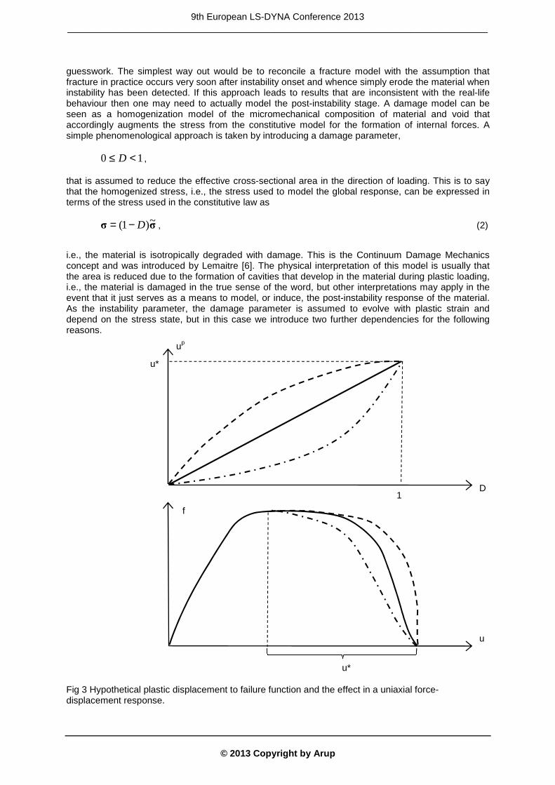
Fig 3 Hypothetical plastic displacement to failure function and the effect in a uniaxial force-displacement response.

u*

u

f

D

up

1

u*



An important aspect is that the resulting strain softening behavior that is induced by a damage model leads to results that depend highly on the numerical discretization, the finite element mesh imposes the size of the obtained localization areas and a coarse mesh is generally less prone to strain localization when compared to a fine mesh. To attenuate this effect a regularization is imperative and this is here done by that the damage parameter is assumed to depend on the mesh size h. Furthermore, in order to accurately model the shape of different engineering stress-strain responses as shown in Fig 3, a dependency on the damage parameter itself is introduced, resulting in a damage evolution law on the form

),,,( hDDD p ηε&&& = . This is further simplified by assuming that the damage evolves with the plastic displacement defined by

pp hu ε&& = (3)

and introduce the plastic strain at failure function

),( Duu pf

pf η= (4)

and the resulting damage evolution as

),( DD

u

uD

pf

p

η∂∂

=&

& . (5)

The interpretation of the plastic strain at failure function is illustrated in a uniaxial tension case (η=1/3) in Fig 3, where the value at D=1 governs the elongation of a test specimen between instability and fracture while the appearance governs the tail shape of the force displacement curve.

3 The DIEM model

The DIEM model is thoroughly treated in the LS-DYNA keyword manual on *MAT_ADD_EROSION [7], and should be read in parallel to the following.

3.1 Combining criteria

The DIEM model allows for an arbitrary number of initiation and evolution criteria to be defined and combined. Assuming that n initiation/evolution types have been defined, damage initiation and evolution history variables �� ∈ �0, ∞� and � ∈ �0,1�, i=1,…n, are introduced for each integration point. These are initially set to zero and then evolve with the deformation of the elements according to rules associated with the specific damage initiation and evolution type chosen. The damage initiation variables do not influence the results but just serve as an indicator for the onset of damage. The damage evolution variables govern the damage in the material and are used to form the global damage ∈ �0,1�. When multiple criteria are active, n>1, each individual criterion can be of maximum, ∈ �� , or multiplicative, ∈ ��, type. The global damage variable is defined as

= max(��, ��)

where

�� = max�∈�� = 1 − ! (1 − �)

�∈��"#$



Now to the evolution of the individual damage initiation and evolution history variables, and for the sake of clarity we skip the superscript i from now on.

3.2 Initiation criteria

3.2.1 Ductile criterion

For the ductile initiation option a function %�& = %�

&(', %(&) represents the plastic strain at onset of damage. Optionally this function can depend on the effective plastic strain rate %(&. The damage initiation history variable evolves according to

�� = ) *%&%�

&+,

-.

3.2.2 Shear criterion

For the shear initiation option a function %�& = %�

&(., %(&) represents the plastic strain at onset of damage. This is a function of a shear stress function defined as

. = (/ + 123)/5

with p being the pressure, q the von Mises equivalent stress and τ the maximum shear stress defined as a function of the principal stress values

5 = 67��89: − 7�;<9:=/2. Introduced here is also the pressure influence parameter ks. Optionally this function can depend on the effective plastic strain rate %(&. The damage initiation history variable evolves according to

�� = ) *%&%�

&+,

-.

3.2.3 MSFLD and FLD criteria

The MSFLD and FLD initiation options are restricted to plane stress shell elements, and only the mid-surface is considered in an attempt to characterize the cross section as a whole. For this a function %�

& = %�&(?, %(&) represents the plastic strain at the onset of damage. Optionally this can function can

also depend on the effective plastic strain rate %(&, which must be positive for the initiation variable to evolve. For the MSFLD criterion, the plastic strain used in this failure criterion is a modified effective plastic strain that only evolves when the pressure is negative, i.e., the material is not affected in compression. The damage initiation history variable evolves according to

�� = max@AB%&%�

&, which should be interpreted as the maximum value up to this point in time. In effect, this means that damage starts evolving as soon as the (modified) plastic strain reaches the critical value. The FLD option differs from the MSFLD option in that the damage initiation history variable evolves just as the ductile and shear criteria, i.e.,

�� = ) *%&%�

&+,

-.

and by that the plastic strain here is not modified by the sign of pressure.



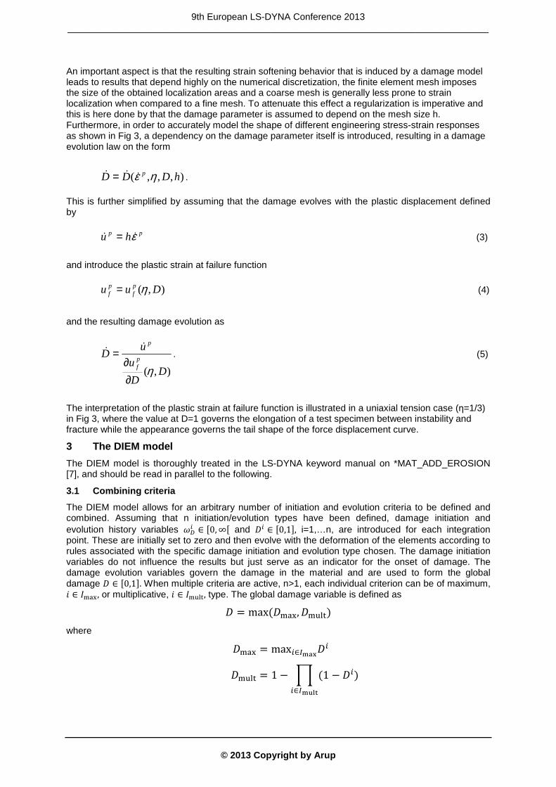
Fig 4 MSFLD input principal stress ratio vs. triaxiality.

The MSFLD (and FLD) instability curve is with respect to the ratio of principal deviatoric stress components in the plane, α, and as a reference we present here the conversion formulae between this quantity and the triaxiality η. This relation is obtained via the following two relations, assuming η>-1/3, and parametrized in β>-1

ββα+

+−=2

12

213

1

βββη++

−=

and is shown in Fig 4. Table 1 lists some of these relations.

3.3 Evolution criteria

For the evolution of the associated damage variable D we introduce the plastic displacement CD which evolves according to

C( & = E0 �� < 1ℎ%(& �� ≥ 1

with h being a characteristic length of the element introduced to suppress the mesh dependence often encountered in finite element damage models. Note that this quantity starts evolving after the corresponding damage initiation variable reaches unity and also that each criterion has its unique plastic displacement variable.

3.3.1 Linear damage evolution

The damage variable evolves linearly with the plastic displacement according to

( = C( &ICJ

&I

with CJ& being the plastic displacement at failure function. The plastic displacement at failure can be

constant or depend on the triaxiality and damage, which in the latter case means that CJ& = CJ

&(', ). This can be used to characterize and differentiate the post-instability stage by designing this function according to the illustration in Fig 3.

-2

-1.5

-1

-0.5

0

0.5

1

-0.4 -0.3 -0.2 -0.1 0 0.1 0.2 0.3 0.4 0.5 0.6 0.7

Alp

ha

Triaxiality



4 Examples

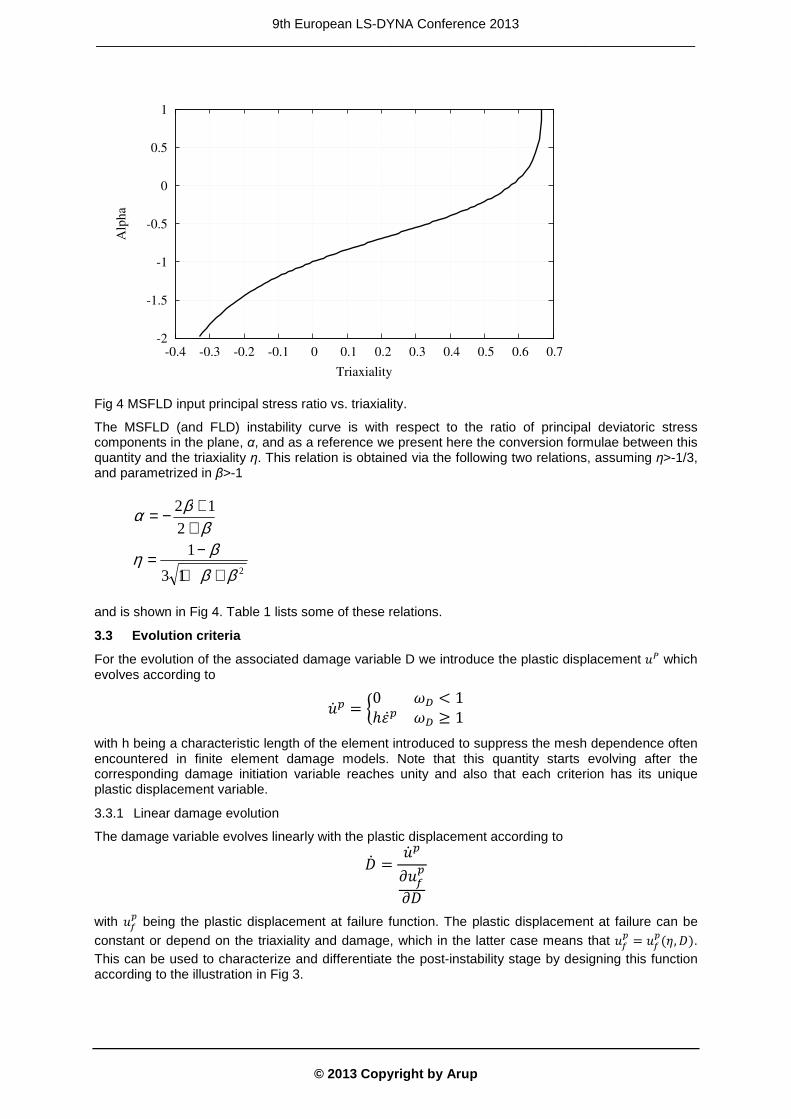
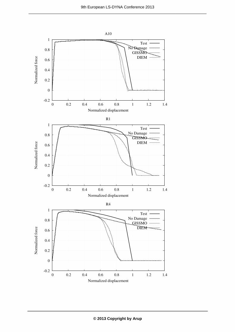
Fig 5 Specimens for calibrating the DIEM model (A10,R4,R1,S0 and S30).

4.1 Crude calibration of the DIEM model

Fig 5 shows some specimens (labeled as in the caption) developed at Fraunhofer IWM, Freiburg, Germany, under the supervision of Dr. Dong-Zhi Sun. When elongated in the vertical direction these are subjected to a reasonably homogenous stress state in the deformation region with triaxiality values as listed in Table 2. The purpose of this example is to design damage initiation and evolution parameters to get the failure characteristics of the aluminium alloy EN-AW 6082 in temper T6 supplied by SAPA. We use the FLD initiation criterion in Section 3.2.3 and want to find the critical plastic strains for the triaxiality values in Table 2, and thereafter use a damage evolution law as in Section 3.3.1 to find the table giving critical plastic displacement as function of triaxiality and damage. Although damage and plastic deformation are two distinct dissipative processes they influence each other, and furthermore the stress state is not homogeneous in the specimens, which makes the calibration of the model non-trivial and an optimization tool such as LS-OPT is generally recommended. The estimation of the DIEM parameters was done manually and intuitively, with results reflecting this fact. Table 2 Rough triaxiality value for the different specimens shown in Fig 5.

Specimen Triaxiality A10 0.33 R4 0.45 R1 0.66 S0 0.0 S30 0.2

In Fig 6, the results from the parameter calibrations for GISSMO and DIEM are shown, of which the former is done with LS-OPT. One immediate conclusion can be drawn, being that a perfect fit to tests for all the specimens is simply out of reach. This can be at least partly attributed to the complex mechanisms occurring in the post-instability region of the different tests, i.e., the coupling and transition between different stress states. A more complex model and better understanding of micromechanical effects are probably needed to obtain a better fit. It can also be seen that the optimization of the GISSMO model leads to a result seemingly different from (and perhaps better than) the DIEM results, which is probably explained by the difference in approach as the latter is obtained through manual tweeking of parameters with lack of systemacy.



-0.2

0

0.2

0.4

0.6

0.8

1

0 0.2 0.4 0.6 0.8 1 1.2 1.4

Norm

aliz

ed f

orc

e

Normalized displacement

A10

Test

No Damage

GISSMO

DIEM

-0.2

0

0.2

0.4

0.6

0.8

1

0 0.2 0.4 0.6 0.8 1 1.2 1.4

Norm

aliz

ed f

orc

e


R1

Test

No Damage

GISSMO

DIEM

-0.2

0

0.2

0.4

0.6

0.8

1

0 0.2 0.4 0.6 0.8 1 1.2 1.4

Norm

aliz

ed f

orc

e


R4

Test

No Damage

GISSMO

DIEM



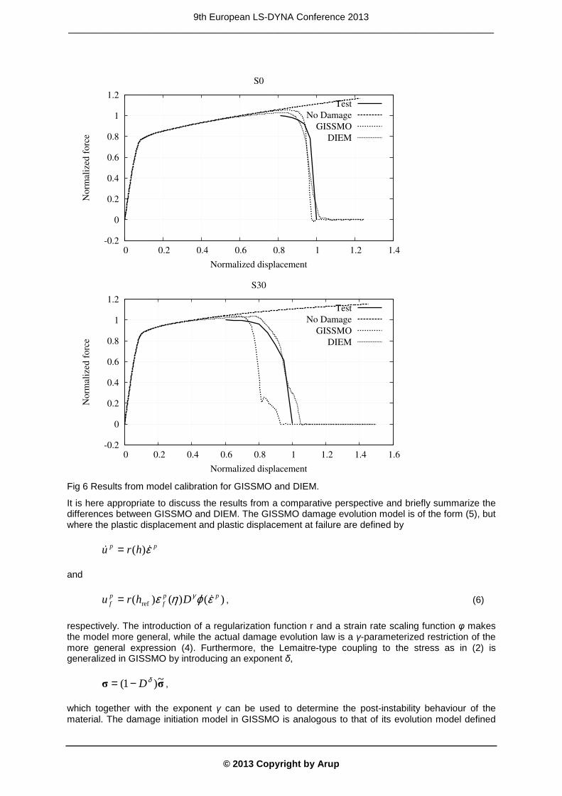
Fig 6 Results from model calibration for GISSMO and DIEM.

It is here appropriate to discuss the results from a comparative perspective and briefly summarize the differences between GISSMO and DIEM. The GISSMO damage evolution model is of the form (5), but where the plastic displacement and plastic displacement at failure are defined by

pp hru ε&& )(= and

)()()( refpp

fpf Dhru εϕηε γ

&= , (6)

respectively. The introduction of a regularization function r and a strain rate scaling function φ makes the model more general, while the actual damage evolution law is a γ-parameterized restriction of the more general expression (4). Furthermore, the Lemaitre-type coupling to the stress as in (2) is generalized in GISSMO by introducing an exponent δ,

σσ~)1( δD−= ,

which together with the exponent γ can be used to determine the post-instability behaviour of the material. The damage initiation model in GISSMO is analogous to that of its evolution model defined

-0.2

0

0.2

0.4

0.6

0.8

1

1.2

0 0.2 0.4 0.6 0.8 1 1.2 1.4

Norm

aliz

ed f

orc

e


S0

Test

No Damage

GISSMO

DIEM

-0.2

0

0.2

0.4

0.6

0.8

1

1.2

0 0.2 0.4 0.6 0.8 1 1.2 1.4 1.6

Norm

aliz

ed f

orc

e


S30

Test

No Damage

GISSMO

DIEM



by (6) except for no element size dependency. The initiation model utilizes the same exponent γ and strain rate scaling function φ as in the evolution model. This should be compared to the DIEM correspondence in (1), which is a simplified variant of the GISSMO counterpart except for a more general strain rate dependence. For linear strain paths they more or less amount to the same thing, but GISSMO allows for more flexibility when it comes to fitting the instability onset for nonlinear strain paths. All in all the two models are similar and regardless of preference, the performance hinges mostly upon how well the damage initation and evolution parameters are fit to reflect the failure characteristics of the material of interest.

4.2 DIEM and CrachFEM

Some single element examples with different strain paths will be used to illustrate the DIEM model and compare it to two alternative failure prediction models: CrachFEM by Matfem [4] and the standard LS-Dyna model MAT190 [7], an anisotropic elastic-plastic material model with a strain based failure criterion. The material used is a relatively brittle high strength steel. Hence failure can be assumed to occur close to instability and therefore only damage initiation is considered. The FLD criterion is used and although the Ductile and Shear criteria are also included in the model, they are never critical.

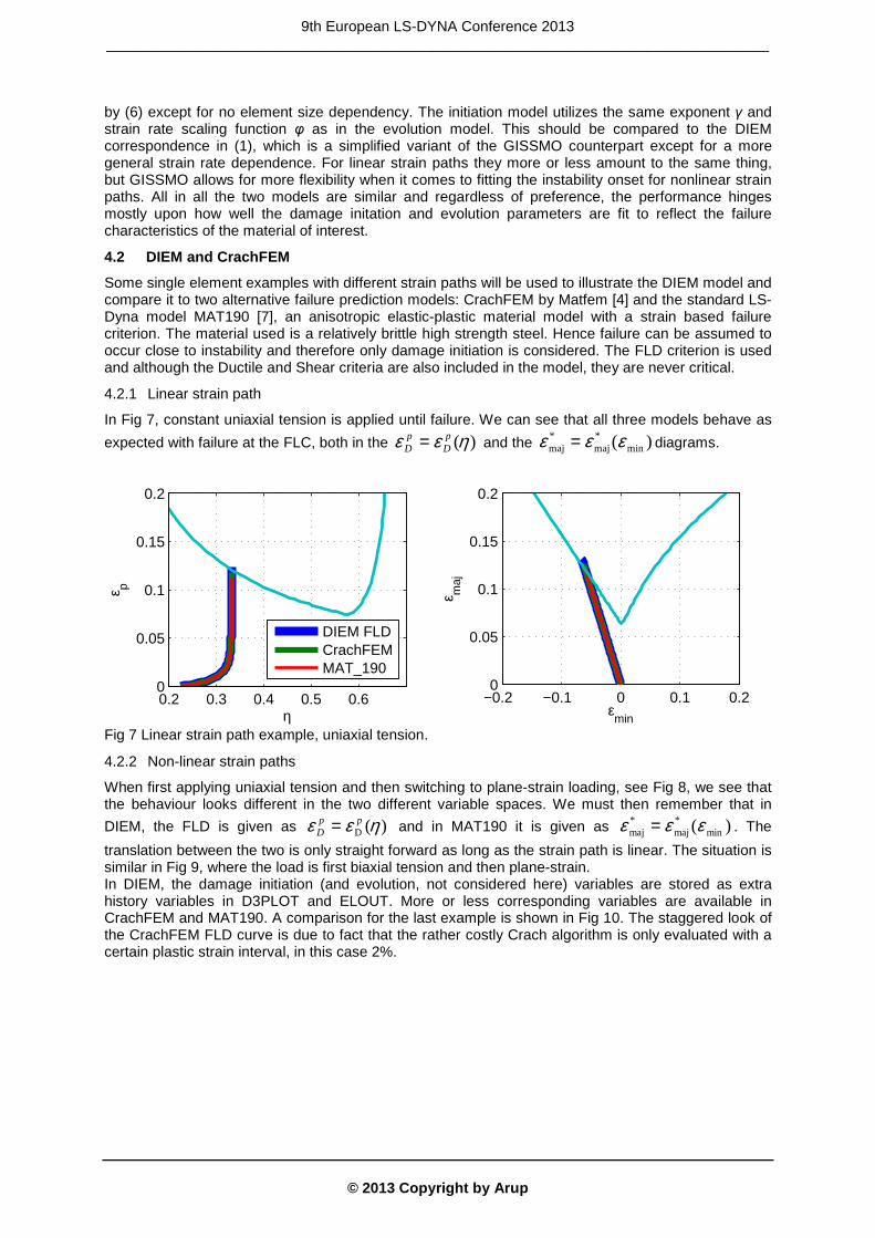
4.2.1 Linear strain path

In Fig 7, constant uniaxial tension is applied until failure. We can see that all three models behave as

expected with failure at the FLC, both in the )(ηεε pD

pD = and the )( min

*maj

*maj εεε = diagrams.

Fig 7 Linear strain path example, uniaxial tension.

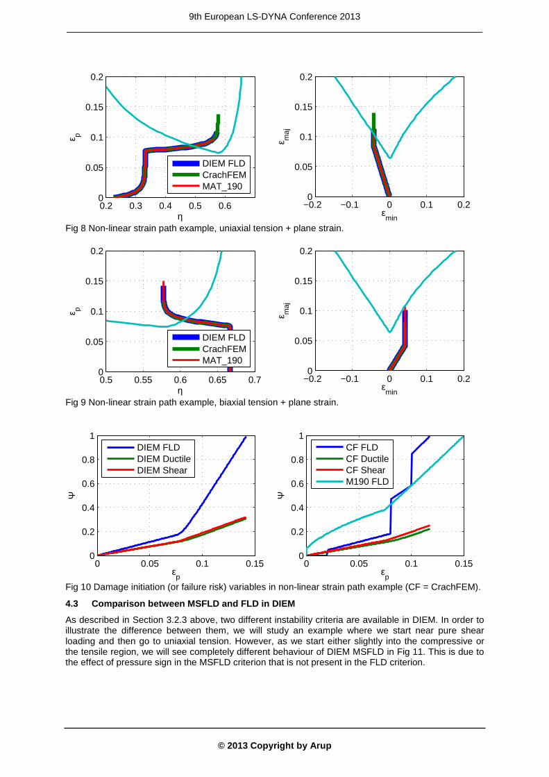
4.2.2 Non-linear strain paths

When first applying uniaxial tension and then switching to plane-strain loading, see Fig 8, we see that the behaviour looks different in the two different variable spaces. We must then remember that in

DIEM, the FLD is given as )(D ηεε ppD = and in MAT190 it is given as )( min

*maj

*maj εεε = . The

translation between the two is only straight forward as long as the strain path is linear. The situation is similar in Fig 9, where the load is first biaxial tension and then plane-strain. In DIEM, the damage initiation (and evolution, not considered here) variables are stored as extra history variables in D3PLOT and ELOUT. More or less corresponding variables are available in CrachFEM and MAT190. A comparison for the last example is shown in Fig 10. The staggered look of the CrachFEM FLD curve is due to fact that the rather costly Crach algorithm is only evaluated with a certain plastic strain interval, in this case 2%.

0.2 0.3 0.4 0.5 0.60

0.05

0.1

0.15

0.2

ε p

η

DIEM FLDCrachFEMMAT_190

−0.2 −0.1 0 0.1 0.20

0.05

0.1

0.15

0.2

εmin

ε maj



Fig 8 Non-linear strain path example, uniaxial tension + plane strain.

Fig 9 Non-linear strain path example, biaxial tension + plane strain.

Fig 10 Damage initiation (or failure risk) variables in non-linear strain path example (CF = CrachFEM).

4.3 Comparison between MSFLD and FLD in DIEM

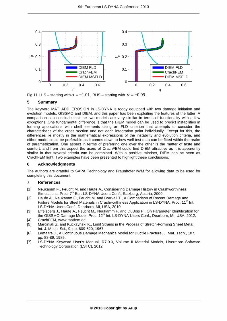
As described in Section 3.2.3 above, two different instability criteria are available in DIEM. In order to illustrate the difference between them, we will study an example where we start near pure shear loading and then go to uniaxial tension. However, as we start either slightly into the compressive or the tensile region, we will see completely different behaviour of DIEM MSFLD in Fig 11. This is due to the effect of pressure sign in the MSFLD criterion that is not present in the FLD criterion.

0.2 0.3 0.4 0.5 0.60

0.05

0.1

0.15

0.2ε p

η


−0.2 −0.1 0 0.1 0.20

0.05

0.1

0.15

0.2

εmin

ε maj

0.5 0.55 0.6 0.65 0.70

0.05

0.1

0.15

0.2

ε p

η


−0.2 −0.1 0 0.1 0.20

0.05

0.1

0.15

0.2

εmin

ε maj

0 0.05 0.1 0.150

0.2

0.4

0.6

0.8

1

εp

Ψ

DIEM FLDDIEM DuctileDIEM Shear

0 0.05 0.1 0.150

0.2

0.4

0.6

0.8

1

εp

Ψ

CF FLDCF DuctileCF ShearM190 FLD



Fig 11 LHS – starting with 01.1−=α , RHS – starting with 99.0−=α .

5 Summary

The keyword MAT_ADD_EROSION in LS-DYNA is today equipped with two damage initiation and evolution models, GISSMO and DIEM, and this paper has been exploiting the features of the latter. A comparison can conclude that the two models are very similar in terms of functionality with a few exceptions. One fundamental difference is that the DIEM model can be used to predict instabilities in forming applications with shell elements using an FLD criterion that attempts to consider the characteristics of the cross section and not each integration point individually. Except for this, the differences lie mostly in the mathematical expressions of the instability and evolution criteria, and either model could be preferable as it comes down to how well test data can be fitted within the realm of parametrization. One aspect in terms of preferring one over the other is the matter of taste and comfort, and from this aspect the users of CrachFEM could find DIEM attractive as it is apparently similar in that several criteria can be combined. With a positive mindset, DIEM can be seen as CrachFEM light. Two examples have been presented to highlight these conclusions.

6 Acknowledgments

The authors are grateful to SAPA Technology and Fraunhofer IWM for allowing data to be used for completing this document.

7 References

[1] Neukamm F., Feucht M. and Haufe A., Considering Damage History in Crashworthiness Simulations, Proc. 7th Eur. LS-DYNA Users Conf., Salzburg, Austria, 2009.

[2] Haufe A., Neukamm F., Feucht M. and Borrvall T., A Comparison of Recent Damage and Failure Models for Steel Materials in Crashworthiness Application in LS-DYNA, Proc. 11th Int. LS-DYNA Users Conf., Dearborn, MI, USA, 2010.

[3] Effelsberg J., Haufe A., Feucht M., Neukamm F. and DuBois P., On Parameter Identification for the GISSMO Damage Model, Proc. 12th Int. LS-DYNA Users Conf., Dearborn, MI, USA, 2012.

[4] CrachFEM, www.matfem.de [5] Marciniak Z. and Kuckzynski K., Limit Strains in the Process of Stretch-Forming Sheet Metal,

Int. J. Mech. Sci., 9, pp. 609-620, 1967. [6] Lemaitre J., A Continuous Damage Mechanics Model for Ductile Fracture, J. Mat. Tech., 107,

pp. 83-89, 1985. [7] LS-DYNA Keyword User’s Manual, R7.0.0, Volume II Material Models, Livermore Software

Technology Corporation (LSTC), 2012.

0 0.2 0.4 0.60

0.1

0.2

0.3

0.4ε p

η

DIEM FLDCrachFEMDIEM MSFLD

0 0.2 0.4 0.60

0.1

0.2

0.3

0.4

ε p

η

DIEM FLDCrachFEMDIEM MSFLD



Drilling rotation constraint for shell elements in implicit and explicit analyses

Tobias Erhart1, Thomas Borrvall2

1Dynamore GmbH, Stuttgart, Germany 2Dynamore Nordic AB, Linköping, Sweden

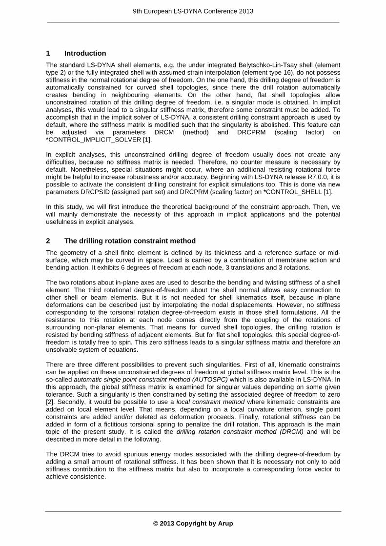
Summary: A subordinate but interesting detail in theory and application of shell elements is investigated in this study, namely the drilling rotation constraint approach. Standard shell elements exhibit 3 translational and 3 rotational degrees-of-freedom at each node. While two nodal rotations are directly associated with bending and twisting modes, the third rotation about the shell normal (also known as the drilling rotation) does not provide any resisting force or stiffness by itself. This fact leads to zero valued components in the stiffness matrix for implicit analyses, which in turn results in a system of equations that cannot be solved. Therefore a small amount of stiffness in form of a torsional spring is artificially added just to remedy the singularity but not to affect the solution too much. This is absolutely necessary to deal with implicit analysis, otherwise no results could be obtained. On the other hand, it might be helpful to have this option also available in explicit analyses to improve results in special situations. It is the intention of this paper to present the theoretical background of this phenomenon and to illustrate the influence of the constraint method in several numerical examples.

Keywords: Shell elements, Drilling degree-of-freedom, Constraint method



1 Introduction The standard LS-DYNA shell elements, e.g. the under integrated Belytschko-Lin-Tsay shell (element type 2) or the fully integrated shell with assumed strain interpolation (element type 16), do not possess stiffness in the normal rotational degree of freedom. On the one hand, this drilling degree of freedom is automatically constrained for curved shell topologies, since there the drill rotation automatically creates bending in neighbouring elements. On the other hand, flat shell topologies allow unconstrained rotation of this drilling degree of freedom, i.e. a singular mode is obtained. In implicit analyses, this would lead to a singular stiffness matrix, therefore some constraint must be added. To accomplish that in the implicit solver of LS-DYNA, a consistent drilling constraint approach is used by default, where the stiffness matrix is modified such that the singularity is abolished. This feature can be adjusted via parameters DRCM (method) and DRCPRM (scaling factor) on *CONTROL_IMPLICIT_SOLVER [1]. In explicit analyses, this unconstrained drilling degree of freedom usually does not create any difficulties, because no stiffness matrix is needed. Therefore, no counter measure is necessary by default. Nonetheless, special situations might occur, where an additional resisting rotational force might be helpful to increase robustness and/or accuracy. Beginning with LS-DYNA release R7.0.0, it is possible to activate the consistent drilling constraint for explicit simulations too. This is done via new parameters DRCPSID (assigned part set) and DRCPRM (scaling factor) on *CONTROL_SHELL [1]. In this study, we will first introduce the theoretical background of the constraint approach. Then, we will mainly demonstrate the necessity of this approach in implicit applications and the potential usefulness in explicit analyses.

2 The drilling rotation constraint method The geometry of a shell finite element is defined by its thickness and a reference surface or mid-surface, which may be curved in space. Load is carried by a combination of membrane action and bending action. It exhibits 6 degrees of freedom at each node, 3 translations and 3 rotations. The two rotations about in-plane axes are used to describe the bending and twisting stiffness of a shell element. The third rotational degree-of-freedom about the shell normal allows easy connection to other shell or beam elements. But it is not needed for shell kinematics itself, because in-plane deformations can be described just by interpolating the nodal displacements. However, no stiffness corresponding to the torsional rotation degree-of-freedom exists in those shell formulations. All the resistance to this rotation at each node comes directly from the coupling of the rotations of surrounding non-planar elements. That means for curved shell topologies, the drilling rotation is resisted by bending stiffness of adjacent elements. But for flat shell topologies, this special degree-of-freedom is totally free to spin. This zero stiffness leads to a singular stiffness matrix and therefore an unsolvable system of equations. There are three different possibilities to prevent such singularities. First of all, kinematic constraints can be applied on these unconstrained degrees of freedom at global stiffness matrix level. This is the so-called automatic single point constraint method (AUTOSPC) which is also available in LS-DYNA. In this approach, the global stiffness matrix is examined for singular values depending on some given tolerance. Such a singularity is then constrained by setting the associated degree of freedom to zero [2]. Secondly, it would be possible to use a local constraint method where kinematic constraints are added on local element level. That means, depending on a local curvature criterion, single point constraints are added and/or deleted as deformation proceeds. Finally, rotational stiffness can be added in form of a fictitious torsional spring to penalize the drill rotation. This approach is the main topic of the present study. It is called the drilling rotation constraint method (DRCM) and will be described in more detail in the following. The DRCM tries to avoid spurious energy modes associated with the drilling degree-of-freedom by adding a small amount of rotational stiffness. It has been shown that it is necessary not only to add stiffness contribution to the stiffness matrix but also to incorporate a corresponding force vector to achieve consistence.



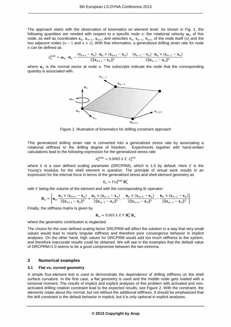
The approach starts with the observation of kinematics on element level. As shown in Fig. 1, the following quantities are needed with respect to a specific node 𝑛: the rotational velocity 𝛚𝑛 of this node, as well as coordinates 𝐱𝑛, 𝐱𝑛−1, 𝐱𝑛+1 and velocities 𝐯𝑛, 𝐯𝑛−1, 𝐯𝑛+1 of the node itself (𝑛) and the two adjacent nodes (𝑛 − 1 and 𝑛 + 1). With that information, a generalized drilling strain rate for node 𝑛 can be defined as

𝜀�̇�drill = 𝛚𝑛 ∙ 𝐧𝑛 −(𝐯𝑛+1 − 𝐯𝑛) ∙ 𝐧𝑛 × (𝐱𝑛+1 − 𝐱𝑛)

2‖𝐱𝑛+1 − 𝐱𝑛‖2−

(𝐯𝑛−1 − 𝐯𝑛) ∙ 𝐧𝑛 × (𝐱𝑛−1 − 𝐱𝑛)2‖𝐱𝑛−1 − 𝐱𝑛‖2

where 𝐧𝑛 is the normal vector at node 𝑛. The subscripts indicate the node that the corresponding quantity is associated with.

Figure 1: Illustration of kinematics for drilling constraint approach

This generalized drilling strain rate is converted into a generalized stress rate by associating a rotational stiffness to the drilling degree of freedom. Experiments together with hand-written calculations lead to the following expression for the generalized stress rate

�̇�𝑛drill = 0.0005 𝑘 𝐸 𝜀�̇�drill

where 𝑘 is a user defined scaling parameter (DRCPRM), which is 1.0 by default. Here 𝐸 is the Young’s modulus for the shell element in question. The principle of virtual work results in an expression for the internal force in terms of the generalized stress and shell element geometry as

𝐟𝑛 = 𝑉𝜎𝑛drill 𝐁𝑛𝑇

with 𝑉 being the volume of the element and with the corresponding B–operator:

𝐁𝑛 = �𝐧𝑛 ,𝐧𝑛 × (𝐱𝑛+1 − 𝐱𝑛)

2‖𝐱𝑛+1 − 𝐱𝑛‖2+𝐧𝑛 × (𝐱𝑛−1 − 𝐱𝑛)

2‖𝐱𝑛−1 − 𝐱𝑛‖2,−

𝐧𝑛 × (𝐱𝑛+1 − 𝐱𝑛)2‖𝐱𝑛+1 − 𝐱𝑛‖2

,−𝐧𝑛 × (𝐱𝑛−1 − 𝐱𝑛)

2‖𝐱𝑛−1 − 𝐱𝑛‖2�

Finally, the stiffness matrix is given by

𝐊𝑛 = 0.005 𝑘 𝐸 𝑉 𝐁𝑛𝑇 𝐁𝑛

where the geometric contribution is neglected.

The choice for the user defined scaling factor DRCPRM will affect the solution in a way that very small values would lead to nearly singular stiffness and therefore poor convergence behavior in implicit analyses. On the other hand, high values for DRCPRM would add too much stiffness to the system, and therefore inaccurate results could be obtained. We will see in the examples that the default value of DRCPRM=1.0 seems to be a good compromise between the two extrema.

3 Numerical examples 3.1 Flat vs. curved geometry

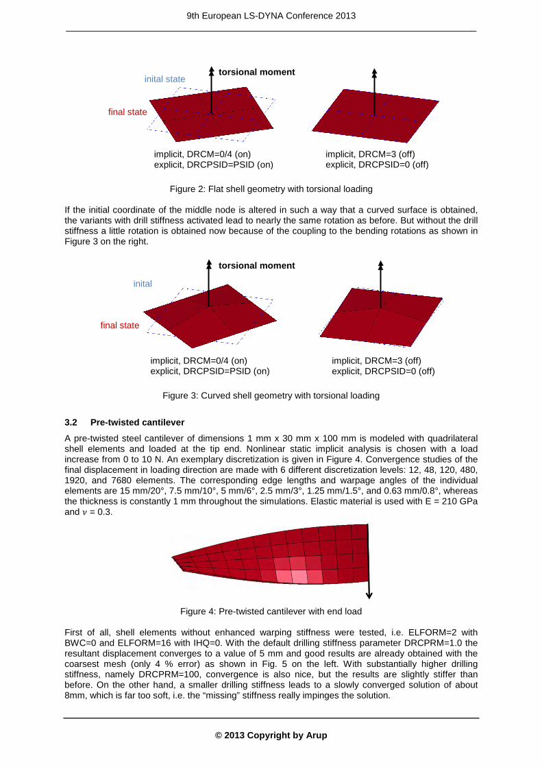
A simple four-element test is used to demonstrate the dependence of drilling stiffness on the shell surface curvature. In the first case, a flat geometry is used and the middle node gets loaded with a torsional moment. The results of implicit and explicit analyses of this problem with activated and non-activated drilling rotation constraint lead to the expected results, see Figure 2. With the constraint, the elements rotate about the normal, but not without the additional stiffness. It should be emphasized that the drill constraint is the default behavior in implicit, but it is only optional in explicit analyses.



Figure 2: Flat shell geometry with torsional loading If the initial coordinate of the middle node is altered in such a way that a curved surface is obtained, the variants with drill stiffness activated lead to nearly the same rotation as before. But without the drill stiffness a little rotation is obtained now because of the coupling to the bending rotations as shown in Figure 3 on the right.

Figure 3: Curved shell geometry with torsional loading

3.2 Pre-twisted cantilever

A pre-twisted steel cantilever of dimensions 1 mm x 30 mm x 100 mm is modeled with quadrilateral shell elements and loaded at the tip end. Nonlinear static implicit analysis is chosen with a load increase from 0 to 10 N. An exemplary discretization is given in Figure 4. Convergence studies of the final displacement in loading direction are made with 6 different discretization levels: 12, 48, 120, 480, 1920, and 7680 elements. The corresponding edge lengths and warpage angles of the individual elements are 15 mm/20°, 7.5 mm/10°, 5 mm/6°, 2.5 mm/3°, 1.25 mm/1.5°, and 0.63 mm/0.8°, whereas the thickness is constantly 1 mm throughout the simulations. Elastic material is used with E = 210 GPa and 𝜈 = 0.3.

Figure 4: Pre-twisted cantilever with end load

First of all, shell elements without enhanced warping stiffness were tested, i.e. ELFORM=2 with BWC=0 and ELFORM=16 with IHQ=0. With the default drilling stiffness parameter DRCPRM=1.0 the resultant displacement converges to a value of 5 mm and good results are already obtained with the coarsest mesh (only 4 % error) as shown in Fig. 5 on the left. With substantially higher drilling stiffness, namely DRCPRM=100, convergence is also nice, but the results are slightly stiffer than before. On the other hand, a smaller drilling stiffness leads to a slowly converged solution of about 8mm, which is far too soft, i.e. the “missing” stiffness really impinges the solution.

torsional moment

implicit, DRCM=0/4 (on) explicit, DRCPSID=PSID (on)

implicit, DRCM=3 (off) explicit, DRCPSID=0 (off)

inital

final state

inital state

final state

implicit, DRCM=0/4 (on) explicit, DRCPSID=PSID (on)

implicit, DRCM=3 (off) explicit, DRCPSID=0 (off)

torsional moment



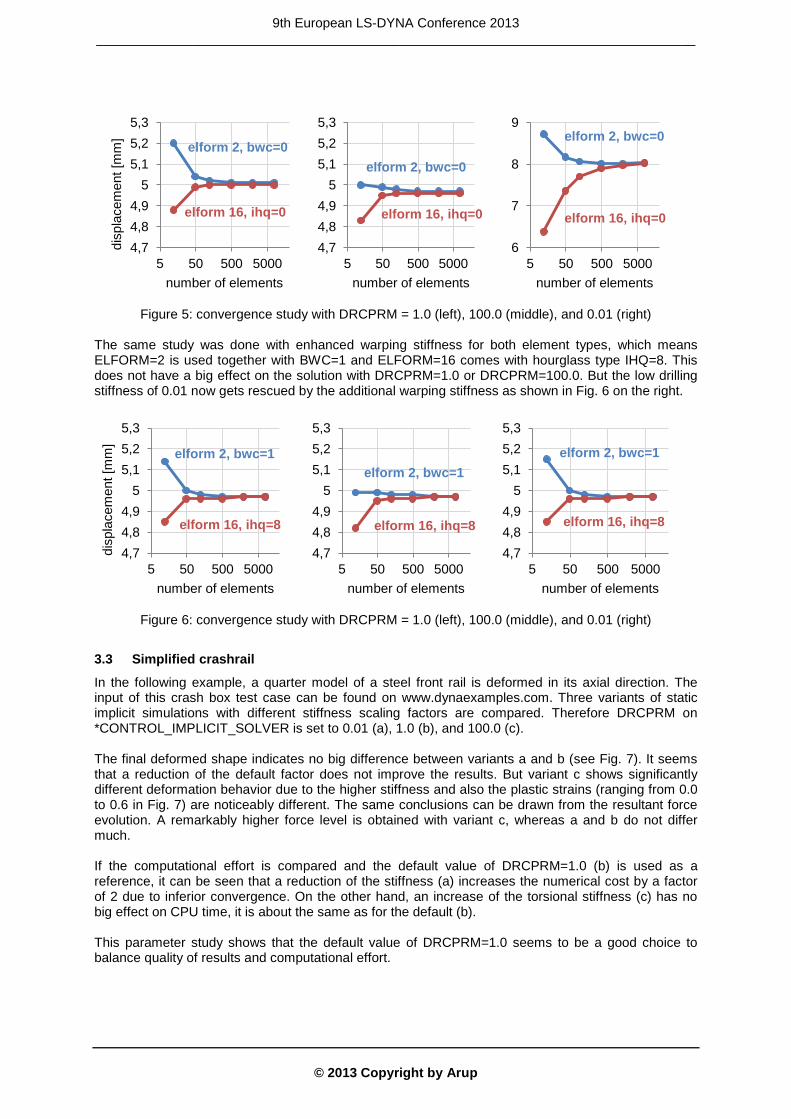
Figure 5: convergence study with DRCPRM = 1.0 (left), 100.0 (middle), and 0.01 (right)

The same study was done with enhanced warping stiffness for both element types, which means ELFORM=2 is used together with BWC=1 and ELFORM=16 comes with hourglass type IHQ=8. This does not have a big effect on the solution with DRCPRM=1.0 or DRCPRM=100.0. But the low drilling stiffness of 0.01 now gets rescued by the additional warping stiffness as shown in Fig. 6 on the right.

Figure 6: convergence study with DRCPRM = 1.0 (left), 100.0 (middle), and 0.01 (right)

3.3 Simplified crashrail

In the following example, a quarter model of a steel front rail is deformed in its axial direction. The input of this crash box test case can be found on www.dynaexamples.com. Three variants of static implicit simulations with different stiffness scaling factors are compared. Therefore DRCPRM on *CONTROL_IMPLICIT_SOLVER is set to 0.01 (a), 1.0 (b), and 100.0 (c). The final deformed shape indicates no big difference between variants a and b (see Fig. 7). It seems that a reduction of the default factor does not improve the results. But variant c shows significantly different deformation behavior due to the higher stiffness and also the plastic strains (ranging from 0.0 to 0.6 in Fig. 7) are noticeably different. The same conclusions can be drawn from the resultant force evolution. A remarkably higher force level is obtained with variant c, whereas a and b do not differ much. If the computational effort is compared and the default value of DRCPRM=1.0 (b) is used as a reference, it can be seen that a reduction of the stiffness (a) increases the numerical cost by a factor of 2 due to inferior convergence. On the other hand, an increase of the torsional stiffness (c) has no big effect on CPU time, it is about the same as for the default (b). This parameter study shows that the default value of DRCPRM=1.0 seems to be a good choice to balance quality of results and computational effort.

4,7 4,8 4,9

5 5,1 5,2 5,3

5 50 500 5000

disp

lace

men

t [m

m]

number of elements

elform 2, bwc=0

elform 16, ihq=0

4,7 4,8 4,9

5 5,1 5,2 5,3

5 50 500 5000 number of elements

elform 2, bwc=0

elform 16, ihq=0

6

7

8

9


elform 2, bwc=0

elform 16, ihq=0

4,7 4,8 4,9

5 5,1 5,2 5,3

5 50 500 5000

disp

lace

men

t [m

m]

number of elements

elform 2, bwc=1

elform 16, ihq=8

4,7 4,8 4,9

5 5,1 5,2 5,3


elform 2, bwc=1

elform 16, ihq=8

4,7 4,8 4,9

5 5,1 5,2 5,3


elform 2, bwc=1

elform 16, ihq=8



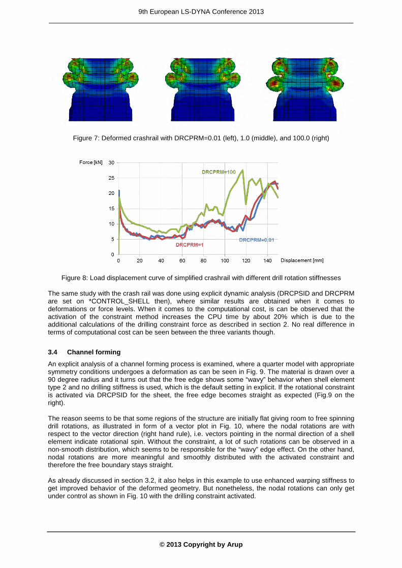
Figure 7: Deformed crashrail with DRCPRM=0.01 (left), 1.0 (middle), and 100.0 (right)

Figure 8: Load displacement curve of simplified crashrail with different drill rotation stiffnesses The same study with the crash rail was done using explicit dynamic analysis (DRCPSID and DRCPRM are set on *CONTROL_SHELL then), where similar results are obtained when it comes to deformations or force levels. When it comes to the computational cost, is can be observed that the activation of the constraint method increases the CPU time by about 20% which is due to the additional calculations of the drilling constraint force as described in section 2. No real difference in terms of computational cost can be seen between the three variants though.

3.4 Channel forming

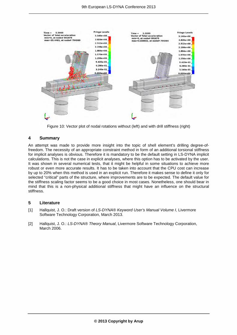
An explicit analysis of a channel forming process is examined, where a quarter model with appropriate symmetry conditions undergoes a deformation as can be seen in Fig. 9. The material is drawn over a 90 degree radius and it turns out that the free edge shows some “wavy” behavior when shell element type 2 and no drilling stiffness is used, which is the default setting in explicit. If the rotational constraint is activated via DRCPSID for the sheet, the free edge becomes straight as expected (Fig.9 on the right). The reason seems to be that some regions of the structure are initially flat giving room to free spinning drill rotations, as illustrated in form of a vector plot in Fig. 10, where the nodal rotations are with respect to the vector direction (right hand rule), i.e. vectors pointing in the normal direction of a shell element indicate rotational spin. Without the constraint, a lot of such rotations can be observed in a non-smooth distribution, which seems to be responsible for the “wavy” edge effect. On the other hand, nodal rotations are more meaningful and smoothly distributed with the activated constraint and therefore the free boundary stays straight. As already discussed in section 3.2, it also helps in this example to use enhanced warping stiffness to get improved behavior of the deformed geometry. But nonetheless, the nodal rotations can only get under control as shown in Fig. 10 with the drilling constraint activated.



Figure 9: Deformation after channel forming process

Figure 10: Vector plot of nodal rotations without (left) and with drill stiffness (right)

3.5 Spot weld connections

Punctual connections between metal parts, e.g. spot welds or rivets, are often discretized by single beam or solid elements fastened to shell element components. The deformation of such an assembled structure leads to local forces and moments acting on the shell elements at the connection point. The nodal rotations of individual nodes in these areas can become important in this context. Often, point-wise connected areas of the structure are geometrically flat in the beginning (e.g. flanges of automotive parts), but they can get highly deformed, i.e. curved and warped, under crash load conditions. For the drilling degrees-of-freedom this means, that torsional rotations are free to spin in the early stages and they can notably be amplified by those local loads. In later stages with ongoing deformation, those rotations can affect the bending behavior around the spot weld, since rotations are coupled in curved geometries as already mentioned above. Usually, this fact does not seem to influence the overall solution. But sometimes, e.g. if unexpectedly large deformations and plastic strains can be seen in the vicinity of such a punctual connection, it could be helpful to activate the drilling constraint for the connected shell parts. To demonstrate the effect of the drill stiffness method in a spot weld assembled structure, a T-bar component test with horizontal impact loading is used. Most differences can be seen when nodal rotations are plotted as vectors as shown in Fig. 11. The spectrum range for the rotations goes from 0 to 3.14 (𝜋) which implies that the maximum is equal to a rotation of 180°. It can be seen that huge rotations take place without the constraint. As already mentioned this is not automatically a problem, because drill rotations do not have an effect in flat geometries. But it is not yet totally understood, what happens when those torsional rotations become coupled with the bending modes during the deformation process, i.e. when the surface becomes curved. At least in this example, the rotations are much smaller if the constraint is activated and local deformations around the spot welds are also decreased resulting in maximum plastic strain changing from 0.36 (w/o constraint) to 0.24 (w/ constraint).



Figure 10: Vector plot of nodal rotations without (left) and with drill stiffness (right)

4 Summary An attempt was made to provide more insight into the topic of shell element’s drilling degree-of-freedom. The necessity of an appropriate constraint method in form of an additional torsional stiffness for implicit analyses is obvious. Therefore it is mandatory to be the default setting in LS-DYNA implicit calculations. This is not the case in explicit analyses, where this option has to be activated by the user. It was shown in several numerical tests, that it might be helpful in some situations to achieve more robust or even more accurate results. It has to be taken into account that the CPU cost can increase by up to 20% when this method is used in an explicit run. Therefore it makes sense to define it only for selected “critical” parts of the structure, where improvements are to be expected. The default value for the stiffness scaling factor seems to be a good choice in most cases. Nonetheless, one should bear in mind that this is a non-physical additional stiffness that might have an influence on the structural stiffness.

5 Literature [1] Hallquist, J. O.: Draft version of LS-DYNA® Keyword User’s Manual Volume I, Livermore

Software Technology Corporation, March 2013. [2] Hallquist, J. O.: LS-DYNA® Theory Manual, Livermore Software Technology Corporation,

March 2006.



A Quadratic Pipe Element in LS-DYNA®

Tobias Olsson, Daniel Hilding

DYNAmore Nordic AB

1 Background Analysis of long piping structures can be challenging due to the enormous number of shell/solid elements that would be required to model a piping structure accurate. In that context a new beam element has been developed that can, if used correctly, reduce the number of elements used in a pipe simulation. Since it is constructed of 3 nodes it is perfect for describing pipe bends, so called elbows. This document is meant as an introduction and modelling techniques for the elbow element. It is implemented in LS-DYNA® R7.0.0 but improvements are implemented in the coming update of LS-DYNA R7 [1].

2 Theory The main theory is based on the work done by Almeida [2] The beam is formulated under the plane stress assumption and with thin shell theory. That means that the quotient between the thickness of the tube (t) and the outer radius (a) should be small and the quotient between the radius and the pipe curvature (R) should also be small. 𝑡𝑎≪ 1, 𝑎

𝑅≪ 1 (1)

The basic assumption is that plane sections originally normal to the center line remain plane but not necessarily normal. The following displacement formula holds for a point in the element after deformation

𝑢𝑖(𝑟, 𝑠, 𝑡) = ∑ ℎ𝑘(𝑟)𝑢𝑖𝑘 + ∑ 𝑎𝑘ℎ𝑘(𝑟)�𝑡𝑉𝑡𝑖𝑘 + 𝑠𝑉𝑠𝑖𝑘�, 𝑖 = 1,2,33𝑘=1

3𝑘=1 (2)

Where 𝑟, 𝑠, 𝑡 are iso-parametric coordinates, 𝑢𝑖 is the displacement at any point in the pipe element, ℎ𝑘 is the interpolation function and 𝑢𝑖𝑘 is the displacement of node 𝑘 in the current element. The 𝑉𝑡𝑖𝑘 and 𝑉𝑠𝑖𝑘 are the components of the rotated orientation vectors along the t and s directions, and 𝑎𝑘 is the outer pipe radius. We calculate 𝑽𝑠𝑘 and 𝑽𝑡𝑘 as the cross product between the nodal rotation increment and the ”old” orientation vector.

𝑽𝑠𝑘 = ∆𝜽𝑘 × 𝑽𝑠0𝑘 (3)

𝑽𝑡𝑘 = ∆𝜽𝑘 × 𝑽𝑡0𝑘 The current beam displacements assume that the cross section of the pipe does not deform. To include the ovalization to the formulation we introduce a new displacement field as follows

𝑤(𝑟,𝜙) = ∑ ∑ ℎ𝑘(𝑟)(𝑐𝑚𝑘 sin 2𝑚𝜙 + 𝑑𝑚𝑘 cos 2𝑚𝜙)3𝑘=1

3𝑚=1 (4)

Where 𝑐𝑚𝑘 and 𝑑𝑚𝑘 are generalized ovalization displacements. The total displacement is calculated as the sum of 𝑢 and 𝑤 which give the beam a total of 12 degrees of freedom per node.



Almeida’s theory is here enhanced with the possibility to include an inner pressure to for example simulate inner or outer loads such as gas pressure or water pressure due to sub sea placement. The inner pressure works two ways. First it works to stiffen the pipe against bending, i.e., reduces the ovalization displacements. Secondly, it adds stress in the axial and circumferential directions by using simple linear pipe equations. The stresses that are transferred and added to the materials are given by: Straight pipe

𝜎𝑟 = 𝑃𝑎𝑚2𝑡

, 𝜎𝑐𝑖𝑟𝑐 = 𝑃𝑎𝑚𝑡

(5)

Curved pipe

𝜎𝑟 = 𝑃𝑎𝑚2𝑡

, 𝜎𝑐𝑖𝑟𝑐 = 𝑃𝑎𝑚2𝑡

2𝑅−𝑎𝑚 cos𝜙𝑅−𝑎𝑚 cos𝜙

, (6)

where 𝑃 is the applied pressure, 𝑎𝑚 is the mean radius of the tube, 𝑅 is the pipe curvature radius and 𝑡 is the pipe thickness.

Fig. 1: Illustration of a pipe beam element, 𝒓, 𝒔 and 𝒕 are position vectors, 𝒂𝒎 is the mean radius of the tube, R is the pipe curvature radius and t is the wall thickness.

3 Modelling The pipe element is constructed of three nodes and an orientation node. And the layout of the pipe is to interpolate a quadratic function through the nodes. The bends should be modeled as circular arcs. The orientation vectors are always constructed such that t is perpendicular to the pipe axis and for a curved pipe pointing at the curvature center or for a straight pipe in the same plane as the orientation node and perpendicular to the pipe axis. The curvature center is automatically calculated and it is assumed that the bend is a part of circle. If the pipe is initially curved the orientation node is set to the curvature center. If a straight pipe is used the orientation node should be set to keep continuity in the t direction between elements. Fig. 2: Pipe beam node orientation.

𝒓

R

𝒔

𝒕 𝑎𝑚 𝑡

N1 N2

N3

O1



3.1 Input example (Element)

The input for a pipe element is almost identical as for an ordinary beam. The difference is that the middle node (N3) is also given on card 1 row 2. Note that the orientation node must always be included even though its coordinates are calculated internally for a curved pipe: *ELEMENT_BEAM_ELBOW $ EID PID NODE1 NODE2 ONODE 1 1 N1 N2 O1 $ NODE3 N3 As a rule of thumbs and for good accuracy it is recommended to use at least 4-6 elements for a 90 degree elbow.

3.2 Input example (Section)

The pipe element is activated by setting the element formulation to 14 in *SECTION_BEAM. Also an integration rule id must be given and the CST parameter should be set to 2. Moreover, the integration rule must be tubular (9). Physical options such as pressure and elongation effects are also given in the section keyword. The pressure is given at card 1 on row 2, the inclusion of end effects are given at card 3 on row 2. Card 2 on row 2 is for output of the ovalization degrees of freedom, that is, 𝑐𝑘 and 𝑑𝑘 as an ASCII-file. Doing so it is possible to visualize the ovalization of the pipe by valuate the ovalization displacements 𝑤(𝑟,𝜙). Below is an example of a section with 1 MPa as internal pressure and both ovalization printing and elongation active. *SECTION_BEAM $ SID ELFORM SHRF QR/IRID CST 1 14 1.0 -1 2.0 $ PR IOVPR IPRSTR 1.0E6 1 1 *INTEGRATION_BEAM $ IRID NIP RA ICST K 1 0 0 9 0 $ D1 D2 1.0 0.7 Also, note the option NEIPB on*DATABASE_EXTENT_BINARY that control the output off the loop stresses. Right now the only option that will work is to set NEIPB to 0 (default) and use the corresponding ASCII-file to fringe plot the loop-stress. All other stresses are of course included in the d3plot file.

3.3 Ovalization degrees of freedom

The extra degrees of freedom are described by scalar nodes that are automatically created during the initialization. Unfortunately that means that the node ids are not known beforehand. However, during the generation of these extra nodes they are echoed to the messag file for easy access for the user. For example, the information can look like this: ELBOW BEAM: 1 n1-n3-n2: 1 2 3 ovalization nodes: 1701 1704 1703 1705 1707 1706 And it means that elbow beam id 1 that is constructed of nodes 1, 2 and 3 were node 3 is the middle node, have the ovalization degrees saved in nodes 1701 to 1707. The 𝑐1, 𝑐2 and 𝑐3 for node 1, 3 and 2 are stored in 1701, 1704 and 1703, and 𝑑1, 𝑑2 and 𝑑3 are stored in 1705, 1707 and 1706. To simulate a cantilever beam the first node should be constrained in all DOFs. In this case that means nodes 1, 1701 and 1705.



If the IOVPR flag is set, then the ovalization displacements for each element are written to an ASCII file ‘elbwov’. They can be used for further analysis of the pipe. For example the total ovalization of the pipe can be calculated by using the displacement formula above. The format for the ASCII file is as follows (spaces have been removed to fit this page): OVALIZATION D.O.F. WITH PRESSURE: 1.210E+06 (TIME = 1.000000) BEAM ID: 1 c1 c2 c3 d1 d2 d3 NODE 1: 0.35E-4 -0.49E-5 0.16E-6 -0.40E-3 -0.19E-4 -0.15E-5 NODE 2: 0.46E-4 0.28E-5 -0.77E-7 0.36E-3 0.23E-4 0.52E-4 NODE 3: 0.11E-3 -0.74E-5 0.14E-6 0.16E-2 -0.84E-4 0.10E-3 Note that the ovalization nodes only have translation degrees of freedom. That means that velocity boundary conditions cannot be set.

3.4 Contacts

Due to the extra node in this formulation the beam contacts will not work for curved beams. If a beam contact is used the curved beam will be treated as a linear beam between node 1 and 2. Node to node contacts and node to surface contacts should work as usual but the curved beam between the nodes will not be added to the contact.

4 Examples In LS-PrePost® 4.1 or newer a new rendering engine is implemented that can visualize the pipes as curved beams, see Fig. 3. All that is needed is that the k-file is used together with the d3plot file and that the CST flag is set to 2.

4.1 Two elements Cantilever beam

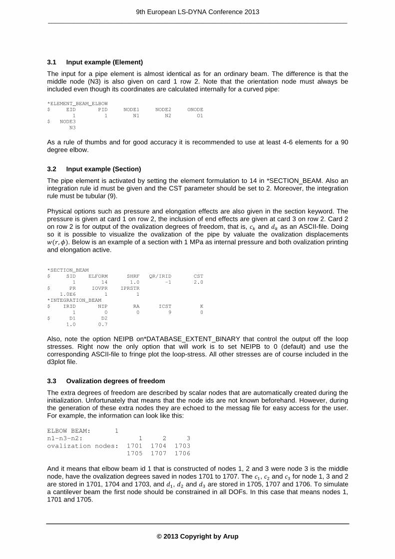
The first example is a simple cantilever beam that is constructed with only 2 elbow elements. The purpose is to do a comparison with the standard beam type 1 and the analytical result that is available in Almeida [2].

Fig. 3: Cantilever beam modeled with 2 elbow elements. To the left is the initial geometry and to the right is the deformed state. The material is linear elastic with a Young’s modulus at 207GPa and Poisson ratio equal to 0.0. The applied torque is 40kNm. The initial straight geometry is deformed by the moment and close to a half-circle is obtained. The same simulation was done with beam type 1 and a comparison between the deformations of the loaded node was done. The result is viewed in Fig. 4 and the simulation with the type 1 beam is not able to complete this test case and is therefore not suitable for this kind of simulations.

Fix

Fix



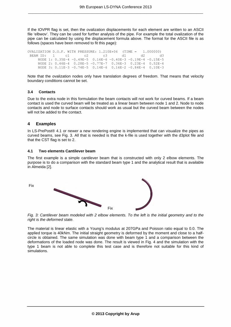
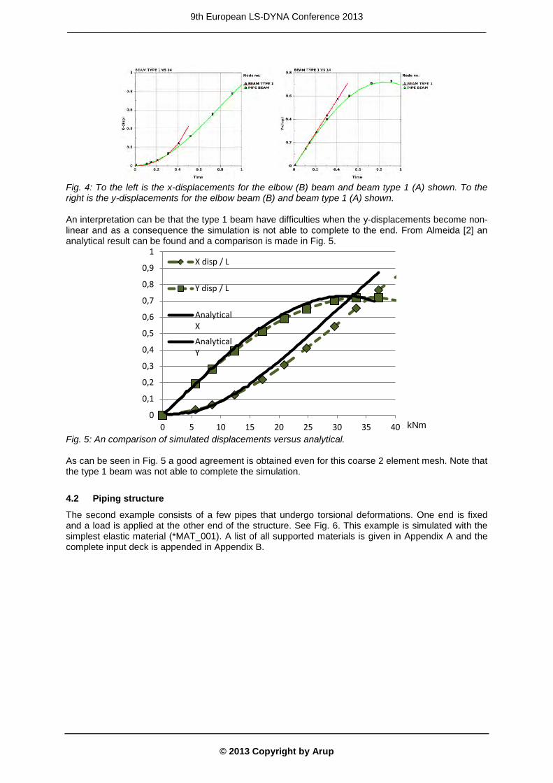
Fig. 4: To the left is the x-displacements for the elbow (B) beam and beam type 1 (A) shown. To the right is the y-displacements for the elbow beam (B) and beam type 1 (A) shown. An interpretation can be that the type 1 beam have difficulties when the y-displacements become non-linear and as a consequence the simulation is not able to complete to the end. From Almeida [2] an analytical result can be found and a comparison is made in Fig. 5.

Fig. 5: An comparison of simulated displacements versus analytical. As can be seen in Fig. 5 a good agreement is obtained even for this coarse 2 element mesh. Note that the type 1 beam was not able to complete the simulation.

4.2 Piping structure

The second example consists of a few pipes that undergo torsional deformations. One end is fixed and a load is applied at the other end of the structure. See Fig. 6. This example is simulated with the simplest elastic material (*MAT_001). A list of all supported materials is given in Appendix A and the complete input deck is appended in Appendix B.

0

0,1

0,2

0,3

0,4

0,5

0,6

0,7

0,8

0,9

1

0 5 10 15 20 25 30 35 40

X disp / L

Y disp / L

Analytical X

Analytical Y

kNm



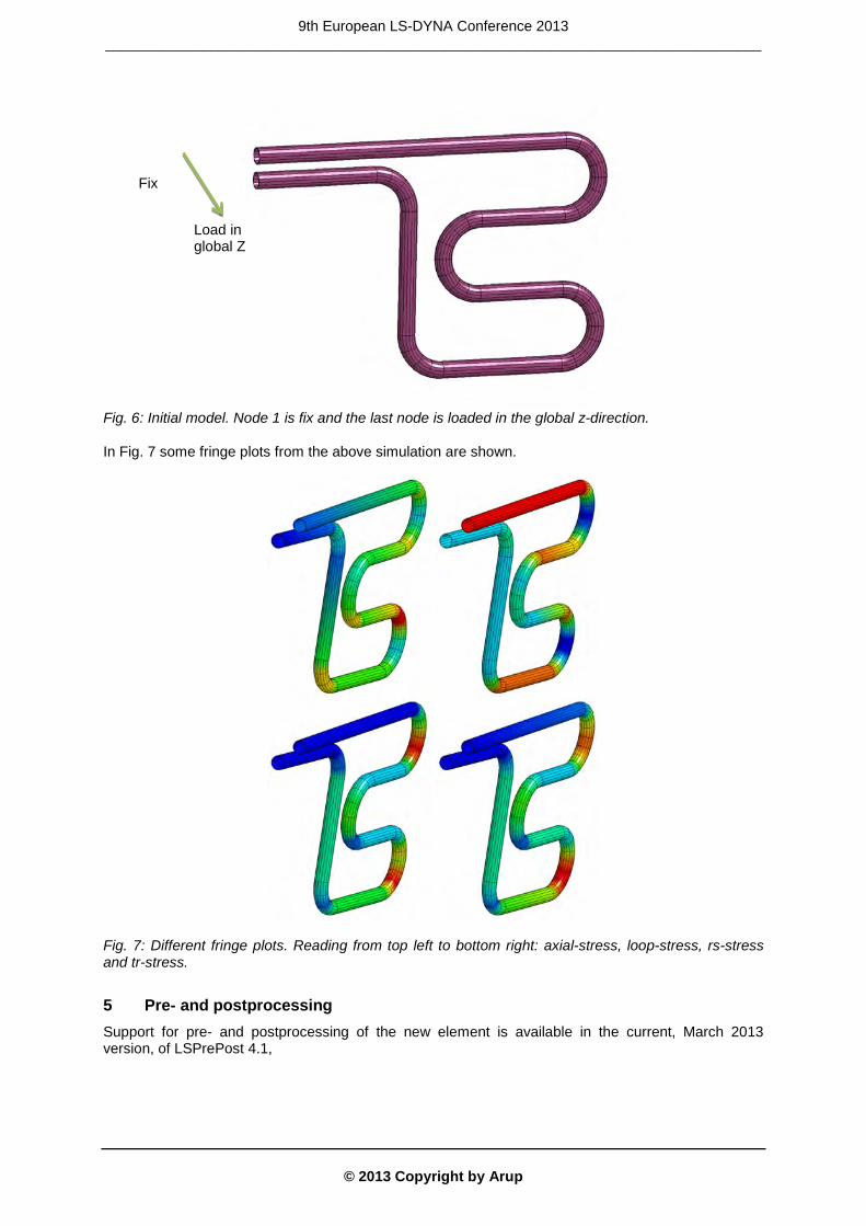
Fig. 6: Initial model. Node 1 is fix and the last node is loaded in the global z-direction. In Fig. 7 some fringe plots from the above simulation are shown.

Fig. 7: Different fringe plots. Reading from top left to bottom right: axial-stress, loop-stress, rs-stress and tr-stress.

5 Pre- and postprocessing Support for pre- and postprocessing of the new element is available in the current, March 2013 version, of LSPrePost 4.1,

Fix

Load in global Z



6 Summary A new beam formulation has been developed and implemented in LS-DYNA R7. It is a 3 node beam with 36 degrees of freedom and quadratic interpolation between nodes. It is tailored for the pipeline and offshore industries but can of course be used in other suitable areas as well. It is cost efficient and accurate.

7 References [1] Hallquist, J. “ LS-DYNA R7.0.0 Keyword User’s Manual – Volume I“, Development version,

Livermore Software Technology Corporation, revision 2999, March 29, Livermore, 2013. [2] Almeida, C.A., “A simple new element for linear and nonlinear analysis of piping systems”, PhD

Thesis, MIT, 1982.

8 Appendix A Currently supported materials (early 2013) are materials number 1, 3, 4, 6, 24,153, and 195.

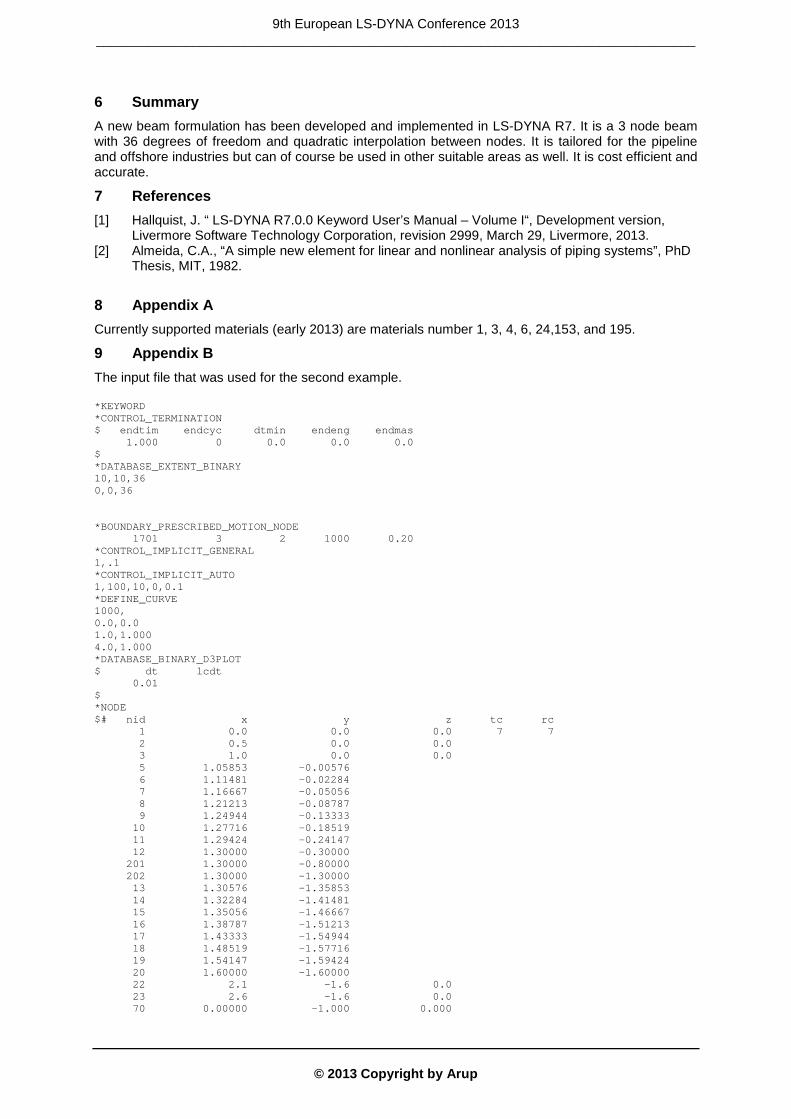
9 Appendix B The input file that was used for the second example. *KEYWORD *CONTROL_TERMINATION $ endtim endcyc dtmin endeng endmas 1.000 0 0.0 0.0 0.0 $ *DATABASE_EXTENT_BINARY 10,10,36 0,0,36 *BOUNDARY_PRESCRIBED_MOTION_NODE 1701 3 2 1000 0.20 *CONTROL_IMPLICIT_GENERAL 1,.1 *CONTROL_IMPLICIT_AUTO 1,100,10,0,0.1 *DEFINE_CURVE 1000, 0.0,0.0 1.0,1.000 4.0,1.000 *DATABASE_BINARY_D3PLOT $ dt lcdt 0.01 $ *NODE $# nid x y z tc rc 1 0.0 0.0 0.0 7 7 2 0.5 0.0 0.0 3 1.0 0.0 0.0 5 1.05853 -0.00576 6 1.11481 -0.02284 7 1.16667 -0.05056 8 1.21213 -0.08787 9 1.24944 -0.13333 10 1.27716 -0.18519 11 1.29424 -0.24147 12 1.30000 -0.30000 201 1.30000 -0.80000 202 1.30000 -1.30000 13 1.30576 -1.35853 14 1.32284 -1.41481 15 1.35056 -1.46667 16 1.38787 -1.51213 17 1.43333 -1.54944 18 1.48519 -1.57716 19 1.54147 -1.59424 20 1.60000 -1.60000 22 2.1 -1.6 0.0 23 2.6 -1.6 0.0 70 0.00000 -1.000 0.000



80 1.00000 -1.30 0.000 90 1.60000 -1.30 0.000 100 2.00000 1.30 0.000 1131 2.6585 -1.5942 1141 2.7148 -1.5772 1151 2.7667 -1.5494 1161 2.8121 -1.5121 1171 2.8494 -1.4667 1181 2.8772 -1.4148 1191 2.8942 -1.3585 1201 2.9000 -1.3000 1211 2.8942 -1.2415 1221 2.8772 -1.1852 1231 2.8494 -1.1333 1241 2.8121 -1.0879 1251 2.7667 -1.0506 1261 2.7148 -1.0228 1271 2.6585 -1.0058 1281 2.6000 -1.0000 1291 2.2500 -1.0000 1301 1.9000 -1.0000 1311 1.8415 -0.9942 1321 1.7852 -0.9771 1331 1.7333 -0.9494 1341 1.6879 -0.9121 1351 1.6506 -0.8667 1361 1.6228 -0.8148 1371 1.6058 -0.7585 1381 1.6000 -0.7000 1391 1.6058 -0.6415 1401 1.6228 -0.5852 1411 1.6506 -0.5333 1421 1.6879 -0.4879 1431 1.7333 -0.4506 1441 1.7852 -0.4228 1451 1.8415 -0.4058 1461 1.9000 -0.4000 1471 2.2500 -0.4000 1481 2.6000 -0.4000 1531 2.6585 -0.3942 1541 2.7148 -0.3772 1551 2.7667 -0.3494 1561 2.8121 -0.3121 1571 2.8494 -0.2667 1581 2.8772 -0.2148 1591 2.8942 -0.1585 1601 2.9000 -0.1000 1611 2.8942 -0.0415 1621 2.8772 0.0148 1631 2.8494 0.0667 1641 2.8121 0.1121 1651 2.7667 0.1494 1661 2.7148 0.1772 1671 2.6585 0.1942 1681 2.6000 .20000 1691 1.3000 .20000 1701 0.0000 .20000 *PART $# title ELBOW PIPE $# pid secid mid 45 45 45 *KEYWORD *ELEMENT_BEAM_ELBOW $ eid pid n1 n2 n5 11 45 1 3 70 2 *ELEMENT_BEAM_ELBOW $ eid pid n1 n2 n5 12 45 3 6 80 5 *ELEMENT_BEAM_ELBOW $ eid pid n1 n2 n5 13 45 6 8 80 7 *ELEMENT_BEAM_ELBOW $ eid pid n1 n2 n5



14 45 8 10 80 9 *ELEMENT_BEAM_ELBOW $ eid pid n1 n2 n5 15 45 10 12 80 11 *ELEMENT_BEAM_ELBOW $ eid pid n1 n2 n5 6 45 12 202 90 201 *ELEMENT_BEAM_ELBOW $ eid pid n1 n2 n5 16 45 202 14 90 13 *ELEMENT_BEAM_ELBOW $ eid pid n1 n2 n5 17 45 14 16 90 15 *ELEMENT_BEAM_ELBOW $ eid pid n1 n2 n5 18 45 16 18 90 17 *ELEMENT_BEAM_ELBOW $ eid pid n1 n2 n5 19 45 18 20 90 19 *ELEMENT_BEAM_ELBOW $ eid pid n1 n2 n5 110 45 20 23 100 22 *ELEMENT_BEAM_ELBOW $ eid pid n1 n2 n5 111 45 23 1141 100 1131 *ELEMENT_BEAM_ELBOW $ eid pid n1 n2 n5 112 45 1141 1161 100 1151 *ELEMENT_BEAM_ELBOW $ eid pid n1 n2 n5 113 45 1161 1181 100 1171 *ELEMENT_BEAM_ELBOW $ eid pid n1 n2 n5 114 45 1181 1201 100 1191 *ELEMENT_BEAM_ELBOW $ eid pid n1 n2 n5 115 45 1201 1221 100 1211 *ELEMENT_BEAM_ELBOW $ eid pid n1 n2 n5 116 45 1221 1241 100 1231 *ELEMENT_BEAM_ELBOW $ eid pid n1 n2 n5 117 45 1241 1261 100 1251 *ELEMENT_BEAM_ELBOW $ eid pid n1 n2 n5 118 45 1261 1281 100 1271 *ELEMENT_BEAM_ELBOW $ eid pid n1 n2 n5 119 45 1281 1301 100 1291 *ELEMENT_BEAM_ELBOW $ eid pid n1 n2 n5 120 45 1301 1321 100 1311 *ELEMENT_BEAM_ELBOW $ eid pid n1 n2 n5 121 45 1321 1341 100 1331 *ELEMENT_BEAM_ELBOW $ eid pid n1 n2 n5 122 45 1341 1361 100



1351 *ELEMENT_BEAM_ELBOW $ eid pid n1 n2 n5 123 45 1361 1381 100 1371 *ELEMENT_BEAM_ELBOW $ eid pid n1 n2 n5 124 45 1381 1401 100 1391 *ELEMENT_BEAM_ELBOW $ eid pid n1 n2 n5 125 45 1401 1421 100 1411 *ELEMENT_BEAM_ELBOW $ eid pid n1 n2 n5 126 45 1421 1441 100 1431 *ELEMENT_BEAM_ELBOW $ eid pid n1 n2 n5 127 45 1441 1461 100 1451 *ELEMENT_BEAM_ELBOW $ eid pid n1 n2 n5 128 45 1461 1481 100 1471 *ELEMENT_BEAM_ELBOW $ eid pid n1 n2 n5 129 45 1481 1541 100 1531 *ELEMENT_BEAM_ELBOW $ eid pid n1 n2 n5 130 45 1541 1561 100 1551 *ELEMENT_BEAM_ELBOW $ eid pid n1 n2 n5 131 45 1561 1581 100 1571 *ELEMENT_BEAM_ELBOW $ eid pid n1 n2 n5 132 45 1581 1601 100 1591 *ELEMENT_BEAM_ELBOW $ eid pid n1 n2 n5 133 45 1601 1621 100 1611 *ELEMENT_BEAM_ELBOW $ eid pid n1 n2 n5 134 45 1621 1641 100 1631 *ELEMENT_BEAM_ELBOW $ eid pid n1 n2 n5 135 45 1641 1661 100 1651 *ELEMENT_BEAM_ELBOW $ eid pid n1 n2 n5 136 45 1661 1681 100 1671 *ELEMENT_BEAM_ELBOW $ eid pid n1 n2 n5 137 45 1681 1701 100 1691 *SECTION_BEAM $ sid elform shrf qr/irid cst 45 14 1.000 -2 2.0 $ PR IOVPR IPRSTR 12.000 1 0 *INTEGRATION_BEAM 2 0 0 9 0 .1375 .125 *MAT_ELASTIC $ mid ro e pr 45 7.86e+3 200.E+9 0.28 *END


FEA Information Engineering Journal - FEAIEJ Information Engineering Journal March... · FEA...

Documents

Transcript of FEA Information Engineering Journal - FEAIEJ Information Engineering Journal March... · FEA...