2010 SIMULIA Customer Conference 1

FEA Capturing Both Brittle and Ductile Crack Propagation

Brian D. Rose1, Ph.D. P.E., Youichi Yamashita2, Ph.D., Ted L. Anderson1

1. Quest Integrity Group, 2. IHI Corporation

, Ph.D., P.E.

Abstract: A finite element analysis methodology was developed to simulate brittle crack initiation, ductile or brittle crack propagation and ductile crack arrest in a single simulation using ABAQUS. Ductile fracture was modeled by employing element deletion when the equivalent plastic strain reached a critical value. Within the same FEM, brittle fracture was modeled by incorporating cohesive behavior between contact surfaces defined along the expected crack face. While this method was not as accurate as an FEM incorporating J integral calculations, its simplicity allowed simultaneous incorporation of brittle and ductile fracture. The material properties for the cohesive behavior at the crack tip were calibrated for crack initiation while the material properties for the remainder of the crack faces were calibrated for crack arrest. Keywords: Crack Propagation, Crack Arrest, Fracture

1. Introduction

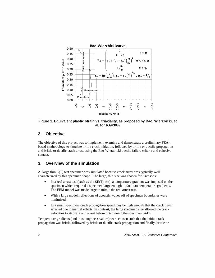
Quest Integrity and IHI implemented and evaluated a new finite element analysis methodology to simulate brittle crack initiation, brittle or ductile crack propagation and brittle or ductile crack arrest in a single simulation using commercially available software. Many current methodologies were available, however none included all the features listed above. For example, Tanguay et al simulated ductile crack propagation using finite element analysis (FEA) and identified a posteriori the crack length corresponding to unstable brittle failure using a modified Weibull stress approach. As another example, Quest Reliability divided the analysis into a sequence of meshes, each with a different crack length and a crack tip spider mesh that facilitated J integral calculation. This approach did not incorporate ductile fracture. For the new methodology developed in this project, ductile crack propagation was modeled by employing element deletion when the equivalent plastic strain reached a critical value. The critical equivalent plastic strain varied with triaxiality, as proposed by Bao, Wierzbicki, et al (see Figure 1). Their method was simple and practical yet accurate. Within the same finite element model (FEM), brittle crack propagation and arrest were modeled using contact defined along the expected crack face, incorporating cohesive traction-separation behavior. While this method was not as accurate as an FEM incorporating J integral calculations, its simplicity allowed simultaneous incorporation of brittle and ductile fracture. The material properties for the cohesive behavior at the crack tip were calibrated for crack initiation while the cohesive material properties for the remainder of the crack were calibrated for crack arrest.

2 2010 SIMULIA Customer Conference

Figure 1. Equivalent plastic strain vs. triaxiality, as proposed by Bao, Wierzbicki, et

al, for RA=30%

2. Objective

The objective of this project was to implement, examine and demonstrate a preliminary FEA-based methodology to simulate brittle crack initiation, followed by brittle or ductile propagation and brittle or ductile crack arrest using the Bao-Wierzbicki ductile failure criteria and cohesive contact.

3. Overview of the simulation

A, large thin C(T) test specimen was simulated because crack arrest was typically well characterized by this specimen shape. The large, thin size was chosen for 3 reasons:

• In a real arrest test (such as the SE(T) test), a temperature gradient was imposed on the specimen which required a specimen large enough to facilitate temperature gradients. The FEM model was made large to mimic the real arrest test.

• With a large model, reflections of acoustic waves off of specimen boundaries were minimized.

• In a small specimen, crack propagation speed may be high enough that the crack never arrested due to inertial effects. In contrast, the large specimen size allowed the crack velocities to stabilize and arrest before out-running the specimen width.

Temperature gradients (and thus toughness values) were chosen such that the initial crack propagation was brittle, followed by brittle or ductile crack propagation and finally, brittle or

0.00

0.05

0.10

0.15

0.20

0.25

0.30

0.35

0.40

0.45

0.50

-1/3 0

1/3

2/3

1

1 1/

3

1 2/

3

2

2 1/

3

2 2/

3

3

3 1/

3

Equi

vale

nt p

last

ic s

trai

n

Triaxiality ratio

Bao-Wierzbicki curve

𝜺𝜺�𝒑𝒑𝒑𝒑 =

⎩⎪⎪⎨

⎪⎪⎧

𝑪𝑪𝟏𝟏𝟏𝟏 + 𝟑𝟑𝟑𝟑

𝟑𝟑 ≤ 𝟎𝟎

𝑪𝑪𝟏𝟏 + (𝑪𝑪𝟐𝟐 − 𝑪𝑪𝟏𝟏) �𝟑𝟑𝟑𝟑𝟎𝟎�𝟐𝟐

𝟎𝟎 < 𝜂𝜂 ≤ 𝟑𝟑𝟎𝟎

𝑪𝑪𝟐𝟐𝟑𝟑𝟎𝟎𝟑𝟑

𝟑𝟑 > 𝟑𝟑𝟎𝟎

� �

𝑪𝑪𝟐𝟐 = 𝒑𝒑𝒍𝒍 � 𝟏𝟏𝟏𝟏−𝑹𝑹𝑹𝑹

�, 𝑪𝑪𝟏𝟏 = 𝑪𝑪𝟐𝟐 �√𝟑𝟑𝟐𝟐�𝟏𝟏 𝒍𝒍�

, 𝟑𝟑 𝟎𝟎 = 𝟏𝟏𝟑𝟑�

Pure shear

Pur

e co

mpr

essi

on

Pure tension

2010 SIMULIA Customer Conference 3

ductile crack arrest. This scenario was chosen because the scenario with ductile initiation followed by brittle propagation was more difficult to simulate as described below. As a ductile crack propagates, the number of potential cleavage nucleation sites experiencing high tensile stresses (characterized by the Weibull stress) increased, according to the Beremin model. When the Weibull stress reached a critical value (i.e. the crack “sampled” a sufficient number of nucleation sites experiencing high stresses), ductile crack propagation changed to brittle crack propagation. To capture this phenomenon, the Weibull stress must be calculated during each FEA increment and a message must be passed to the material model for each cohesive material point, indicating the onset of brittle propagation. Implementing this message passing in the finite element software would have required efforts beyond the scope of this project. To avoid the above described difficulty, this project was limited to the simulation of brittle initiation followed by brittle or ductile arrest. To ensure this sequence, the simulated structure was subjected to a temperature gradient (colder at the crack initiation location, warmer at arrest location), much like the SE(T) test and temperature dependent toughness was incorporated into the model.

4. Material properties

ASTM A533B steel was chosen as the material for this project because this material has been researched extensively and therefore the material properties were readily available.

4.1 Mechanical properties

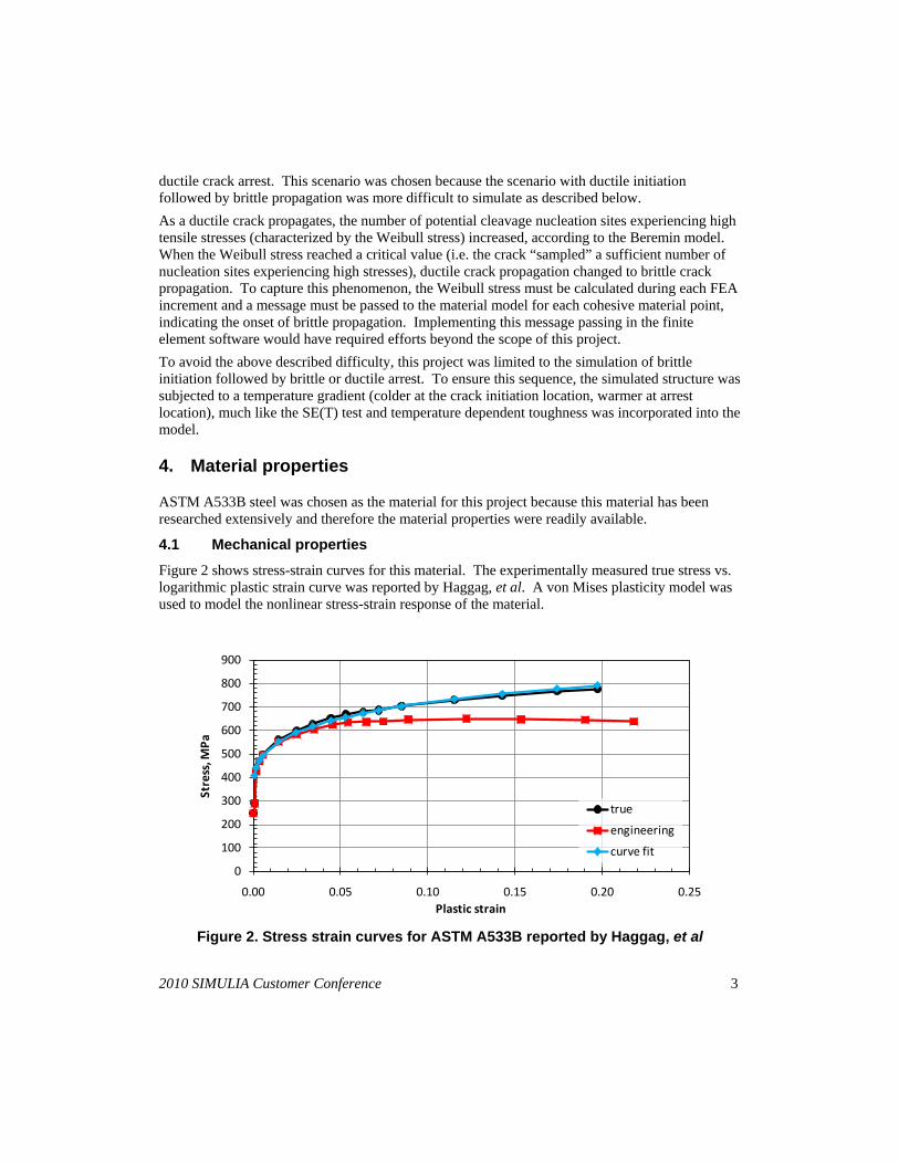
Figure 2 shows stress-strain curves for this material. The experimentally measured true stress vs. logarithmic plastic strain curve was reported by Haggag, et al. A von Mises plasticity model was used to model the nonlinear stress-strain response of the material.

Figure 2. Stress strain curves for ASTM A533B reported by Haggag, et al

0

100

200

300

400

500

600

700

800

900

0.00 0.05 0.10 0.15 0.20 0.25

Stre

ss, M

Pa

Plastic strain

true

engineering

curve fit

4 2010 SIMULIA Customer Conference

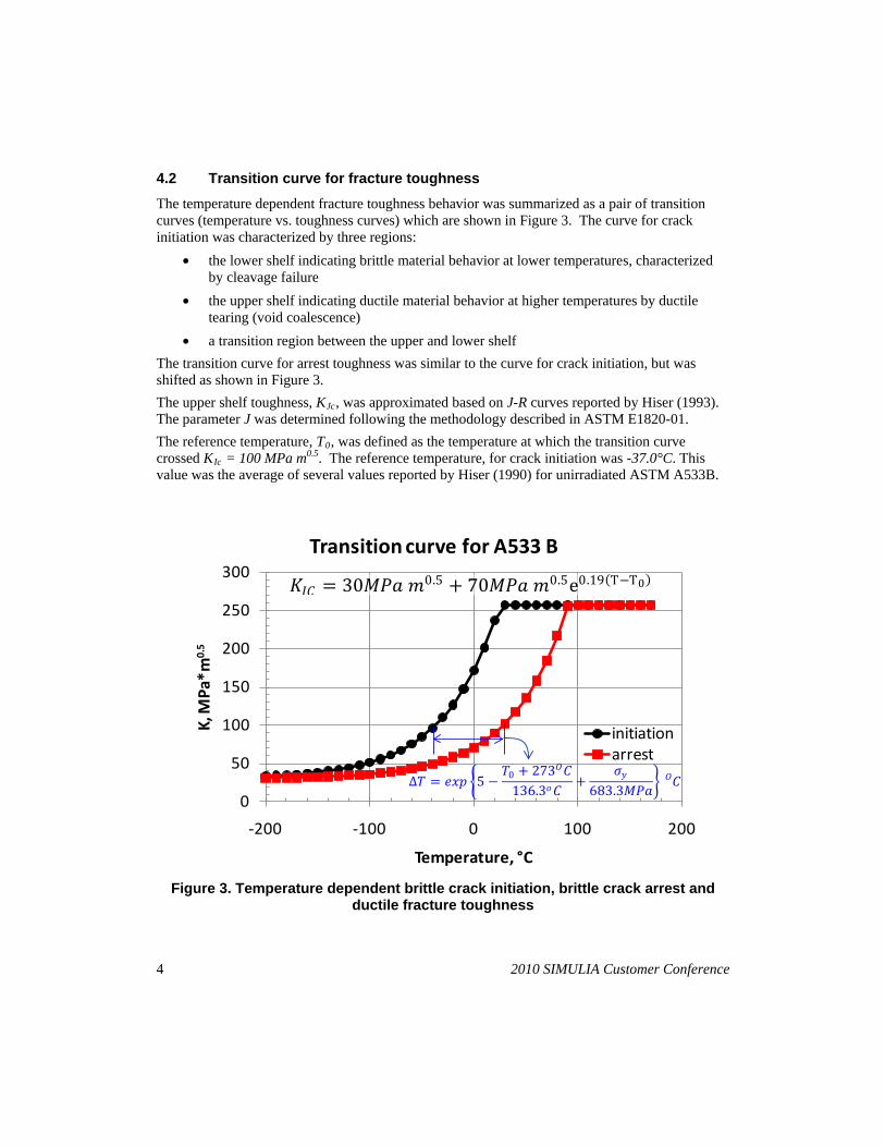
4.2 Transition curve for fracture toughness The temperature dependent fracture toughness behavior was summarized as a pair of transition curves (temperature vs. toughness curves) which are shown in Figure 3. The curve for crack initiation was characterized by three regions:

• the lower shelf indicating brittle material behavior at lower temperatures, characterized by cleavage failure

• the upper shelf indicating ductile material behavior at higher temperatures by ductile tearing (void coalescence)

• a transition region between the upper and lower shelf The transition curve for arrest toughness was similar to the curve for crack initiation, but was shifted as shown in Figure 3. The upper shelf toughness, KJc

The reference temperature, T

, was approximated based on J-R curves reported by Hiser (1993). The parameter J was determined following the methodology described in ASTM E1820-01.

0, was defined as the temperature at which the transition curve crossed KIc = 100 MPa m0.5

. The reference temperature, for crack initiation was -37.0°C. This value was the average of several values reported by Hiser (1990) for unirradiated ASTM A533B.

Figure 3. Temperature dependent brittle crack initiation, brittle crack arrest and

ductile fracture toughness

0

50

100

150

200

250

300

-200 -100 0 100 200

K, M

Pa*m

0.5

Temperature, °C

Transition curve for A533 B

initiationarrest

𝐾𝐾𝐼𝐼𝐼𝐼 = 30𝑀𝑀𝑀𝑀𝑀𝑀 𝑚𝑚0.5 + 70𝑀𝑀𝑀𝑀𝑀𝑀 𝑚𝑚0.5e0.19(T−T0)

Δ𝑇𝑇 = 𝑒𝑒𝑒𝑒𝑒𝑒 �5 −𝑇𝑇0 + 273𝑂𝑂𝐼𝐼

136.3𝑜𝑜𝐼𝐼+

𝜎𝜎𝑦𝑦683.3𝑀𝑀𝑀𝑀𝑀𝑀

� 𝐼𝐼𝑂𝑂

2010 SIMULIA Customer Conference 5

The transition curve for crack initiation was calculated from T0 using the equation described in ASTM E1921-05. The transition curve for crack arrest was calculated from the transition curve for crack initiation. The relationship between crack arrest and initiation was described by Wallin as a shift of T0

4.3 Bao-Wierzbicki model for ductile fracture

. The shift was 65.4°C and the corresponding transition temperature for crack arrest was 28.4°C.

The Bao-Wierzbicki model (equivalent plastic strain vs. triaxiality curve), was calibrated so that KI at crack initiation calculated from simulation and KIc

Figure 2

from experiment matched. Jeong et al provided an approximation of the Bao-Wierzbicki curve (to be used when the experimentally measured curve is not available), in which RA was the reduction of area at fracture of a tensile test specimen and n was the hardening exponent of the stress-strain response as shown in . The RA value was tuned so that FEM and experimental results for ductile fracture matched, resulting in RA=30%. The tuning process is described in a later section. In contrast, Chaouadi and Fabry reported RA=59%. This discrepancy is a well know phenomenon known as localization or mesh size sensitivity: in an FEA, simulated necking typically localizes to one or two elements in an FEA. In an experiment, necking length is material and geometry dependent. RA is closely related to the necking length and therefore RA differs between FEM and experiment.

5. Finite element model

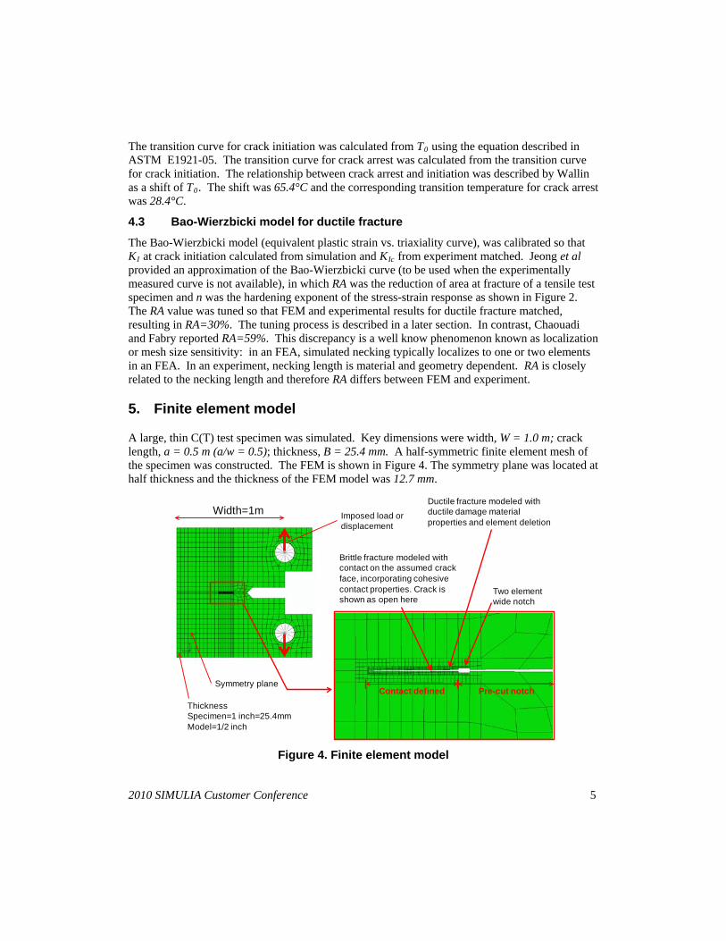
A large, thin C(T) test specimen was simulated. Key dimensions were width, W = 1.0 m; crack length, a = 0.5 m (a/w = 0.5); thickness, B = 25.4 mm. A half-symmetric finite element mesh of the specimen was constructed. The FEM is shown in Figure 4. The symmetry plane was located at half thickness and the thickness of the FEM model was 12.7 mm.

Figure 4. Finite element model

Width=1m

ThicknessSpecimen=1 inch=25.4mmModel=1/2 inch

Symmetry plane

Imposed load or displacement

Ductile fracture modeled with ductile damage material properties and element deletion

Brittle fracture modeled with contact on the assumed crack face, incorporating cohesive contact properties. Crack is shown as open here

Pre-cut notchContact defined

Two element wide notch

6 2010 SIMULIA Customer Conference

Brittle crack propagation and arrest was modeled using contact defined along the expected crack face, incorporating cohesive traction-separation behavior. The mesh was fine on either side of the “contact” faces with the mesh size increasing away from the “contact” faces. The element size in the fine mesh zone was 1.41 mm (9 elements through half thickness). Real specimens are “pulled apart” by loading pins that slip into to the holes of the specimen. In the FEM, the loading pins were modeled as reference nodes that were kinematically coupled (rigidly attached) to the inner surface of the load pin hole. Out of plane displacements on one face of the model were restrained to implement half-symmetry. Loads were applied over a time period ranging from 0.1 to 0.12 seconds. This load duration was chosen to achieve reasonable computer run times. The simulation was performed using an explicit solver because an implicit solver would have diverged due to the incorporated brittle material behavior and element deletion. Noisy results due to acoustic effects were unavoidable and added extra effort for post-processing. Constant mass scaling was used to decrease computer run times. The effect of mass scaling was not investigated but was expected to be minimal.

5.1 Implementation of fracture behavior

Ductile fracture was simulated using the following features (keywords) in Abaqus: *PLASTIC *DAMAGE INITIATION, CRITERION=DUCTILE *DAMAGE EVOLUTION, TYPE=ENERGY

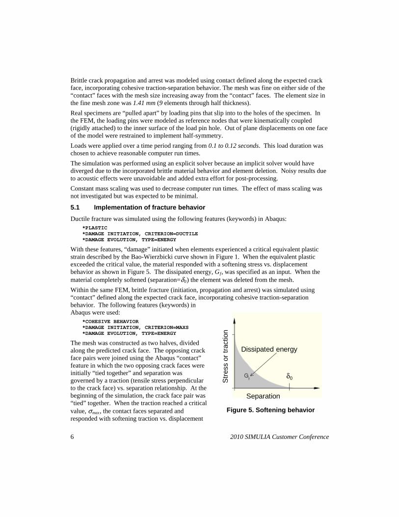
With these features, “damage” initiated when elements experienced a critical equivalent plastic strain described by the Bao-Wierzbicki curve shown in Figure 1. When the equivalent plastic exceeded the critical value, the material responded with a softening stress vs. displacement behavior as shown in Figure 5. The dissipated energy, Gf, was specified as an input. When the material completely softened (separation=δ0

Within the same FEM, brittle fracture (initiation, propagation and arrest) was simulated using “contact” defined along the expected crack face, incorporating cohesive traction-separation behavior. The following features (keywords) in Abaqus were used:

) the element was deleted from the mesh.

*COHESIVE BEHAVIOR *DAMAGE INITIATION, CRITERION=MAXS *DAMAGE EVOLUTION, TYPE=ENERGY

The mesh was constructed as two halves, divided along the predicted crack face. The opposing crack face pairs were joined using the Abaqus “contact” feature in which the two opposing crack faces were initially “tied together” and separation was governed by a traction (tensile stress perpendicular to the crack face) vs. separation relationship. At the beginning of the simulation, the crack face pair was “tied” together. When the traction reached a critical value, σmax, the contact faces separated and responded with softening traction vs. displacement

Figure 5. Softening behavior

Separation

Stre

ss o

r tra

ctio

n

Dissipated energy

δ0

2010 SIMULIA Customer Conference 7

behavior as shown in Figure 5. Note that both ductile softening and cohesive behavior employ the same softening (“damage”) model.

6. Material parameter calibration

Parameters for the material models were calibrated by matching simulated toughness results and experimental results. The following formulas from ASTM E1820-01 were used to correlate load(P), and toughness (KIc or KJc

6.1 Ductile fracture

):

𝐾𝐾𝐼𝐼 =𝑀𝑀

𝐵𝐵√𝑊𝑊𝑓𝑓�

𝑀𝑀𝑊𝑊�

𝑓𝑓 �𝑀𝑀𝑊𝑊� = �

1 + 𝑀𝑀𝑊𝑊

1 − 𝑀𝑀𝑊𝑊�

2

�2.163 + 12.219 �𝑀𝑀𝑊𝑊�−20.065 �

𝑀𝑀𝑊𝑊�

2+0.9925 �

𝑀𝑀𝑊𝑊�

3+20.609 �

𝑀𝑀𝑊𝑊�

4+9.9314 �

𝑀𝑀𝑊𝑊�

5�

The ductile damage parameters (RA, Gf) were calibrated so that KJc from simulations matched the experimentally measured upper shelf toughness. Fracture initiation was defined as the instant when the first element was deleted from the mesh. The calibration results were RA=30% and Gf

6.2 Brittle fracture

= 10 kJ (arbitrarily assumed). The load-displacement curve exhibited ductile response: the load continued to increase (with increased displacement) beyond crack initiation. On the free face, shear lips formed.

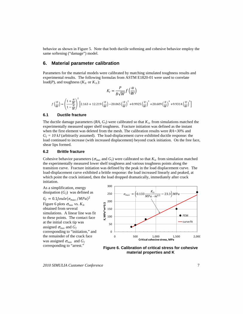
Cohesive behavior parameters (σmax and Gf) were calibrated so that KIc

As a simplification, energy dissipation (G

from simulation matched the experimentally measured lower shelf toughness and various toughness points along the transition curve. Fracture initiation was defined by the peak in the load displacement curve. The load-displacement curve exhibited a brittle response: the load increased linearly and peaked, at which point the crack initiated, then the load dropped dramatically, immediately after crack initiation.

f

𝐺𝐺𝑓𝑓 = 0.1𝐽𝐽𝑜𝑜𝐽𝐽𝐽𝐽𝑒𝑒(𝜎𝜎𝑚𝑚𝑀𝑀𝑒𝑒 𝑀𝑀𝑀𝑀𝑀𝑀⁄ )2 ) was defined as

Figure 6 plots σmax vs. KIc obtained from several simulations. A linear line was fit to these points. The contact face at the initial crack tip was assigned σmax and Gf corresponding to “initiation,” and the remainder of the crack face was assigned σmax and Gf corresponding to “arrest.”

Figure 6. Calibration of critical stress for cohesive

material properties and K

0

50

100

150

200

250

300

0 500 1,000 1,500 2,000

K, M

Pa*m

^0.5

Critical cohesive stress, MPa

FEM

curve fit

𝜎𝜎𝑚𝑚𝑀𝑀𝑒𝑒 = �0.133𝐾𝐾𝐼𝐼𝐼𝐼

𝑀𝑀𝑀𝑀𝑀𝑀 ∙ 𝑚𝑚0.5 − 23.3�𝑀𝑀𝑀𝑀𝑀𝑀

8 2010 SIMULIA Customer Conference

7. Crack arrest simulations

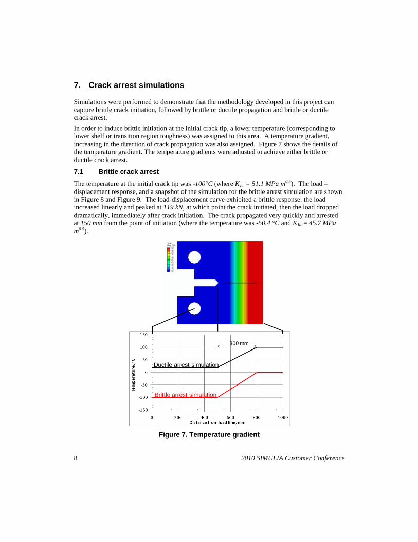
Simulations were performed to demonstrate that the methodology developed in this project can capture brittle crack initiation, followed by brittle or ductile propagation and brittle or ductile crack arrest. In order to induce brittle initiation at the initial crack tip, a lower temperature (corresponding to lower shelf or transition region toughness) was assigned to this area. A temperature gradient, increasing in the direction of crack propagation was also assigned. Figure 7 shows the details of the temperature gradient. The temperature gradients were adjusted to achieve either brittle or ductile crack arrest.

7.1 Brittle crack arrest

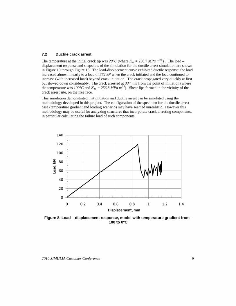
The temperature at the initial crack tip was -100°C (where KIc = 51.1 MPa m0.5

Figure 8

). The load – displacement response, and a snapshot of the simulation for the brittle arrest simulation are shown in and Figure 9. The load-displacement curve exhibited a brittle response: the load increased linearly and peaked at 119 kN, at which point the crack initiated, then the load dropped dramatically, immediately after crack initiation. The crack propagated very quickly and arrested at 150 mm from the point of initiation (where the temperature was -50.4 °C and KIa = 45.7 MPa m0.5

).

Figure 7. Temperature gradient

300 mm

Ductile arrest simulation

Brittle arrest simulation

2010 SIMULIA Customer Conference 9

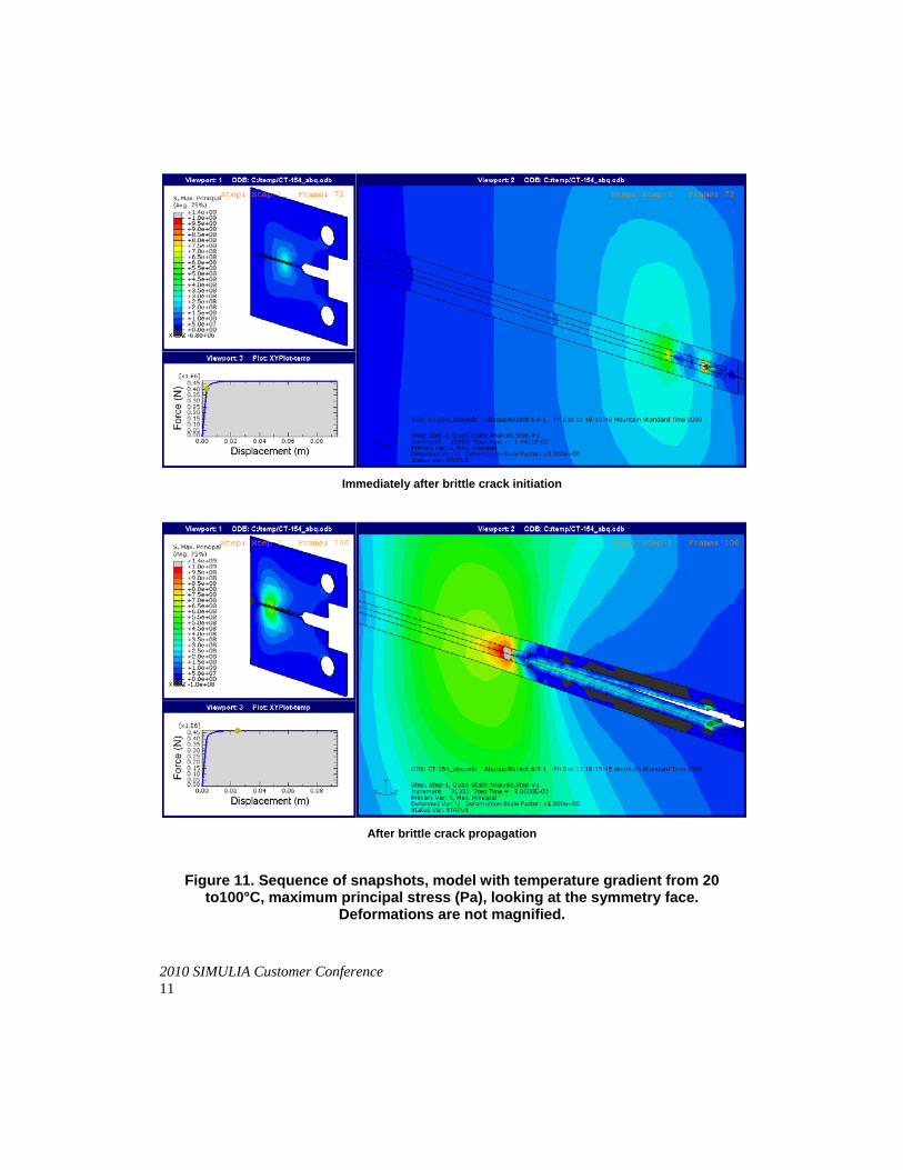
7.2 Ductile crack arrest

The temperature at the initial crack tip was 20°C (where KIc = 236.7 MPa m0.5

Figure 10

) . The load – displacement response and snapshots of the simulation for the ductile arrest simulation are shown in through Figure 13. The load-displacement curve exhibited ductile response: the load increased almost linearly to a load of 382 kN when the crack initiated and the load continued to increase (with increased load) beyond crack initiation. The crack propagated very quickly at first but slowed down considerably. The crack arrested at 334 mm from the point of initiation (where the temperature was 100°C and KIa = 256.8 MPa m0.5

This simulation demonstrated that initiation and ductile arrest can be simulated using the methodology developed in this project. The configuration of the specimen for the ductile arrest case (temperature gradient and loading scenario) may have seemed unrealistic. However this methodology may be useful for analyzing structures that incorporate crack arresting components, in particular calculating the failure load of such components.

). Shear lips formed in the vicinity of the crack arrest site, on the free face.

Figure 8. Load – displacement response, model with temperature gradient from -

100 to 0°C

0

20

40

60

80

100

120

140

0 0.2 0.4 0.6 0.8 1 1.2 1.4

Load

, kN

Displacement, mm

10 2010 SIMULIA Customer Conference

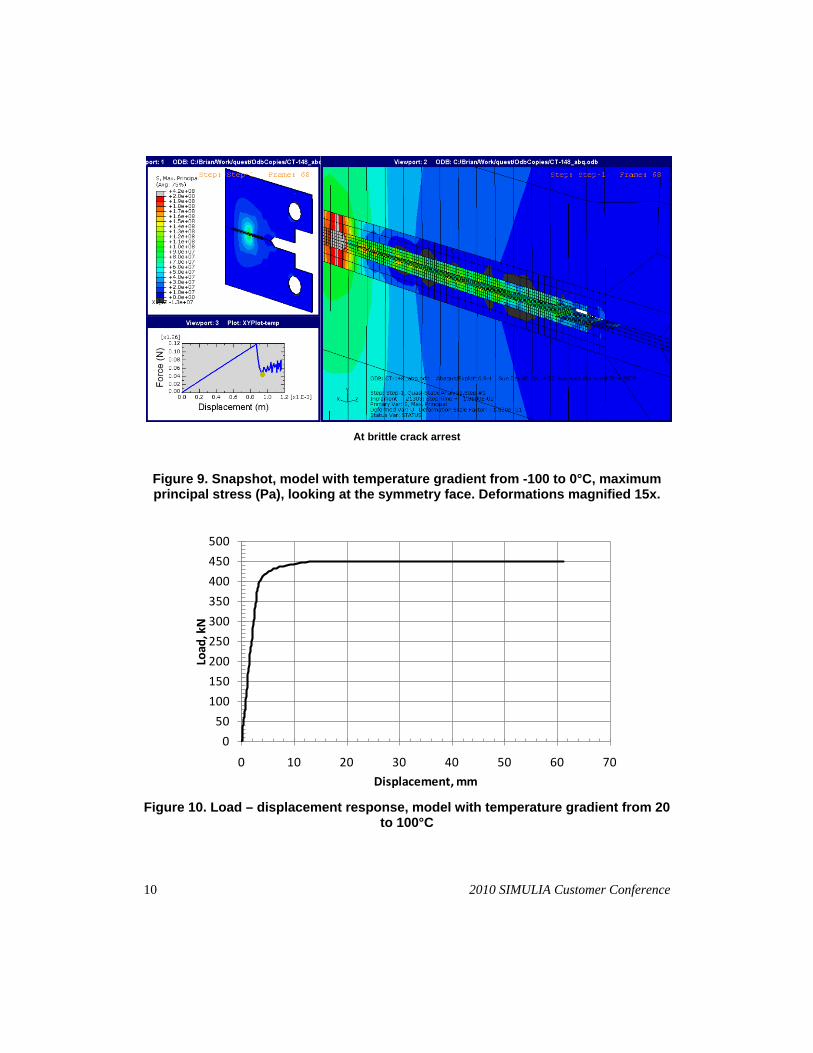
At brittle crack arrest

Figure 9. Snapshot, model with temperature gradient from -100 to 0°C, maximum principal stress (Pa), looking at the symmetry face. Deformations magnified 15x.

Figure 10. Load – displacement response, model with temperature gradient from 20

to 100°C

0

50

100

150

200

250

300

350

400

450

500

0 10 20 30 40 50 60 70

Load

, kN

Displacement, mm

2010 SIMULIA Customer Conference 11

Immediately after brittle crack initiation

After brittle crack propagation

Figure 11. Sequence of snapshots, model with temperature gradient from 20 to100°C, maximum principal stress (Pa), looking at the symmetry face.

Deformations are not magnified.

12 2010 SIMULIA Customer Conference

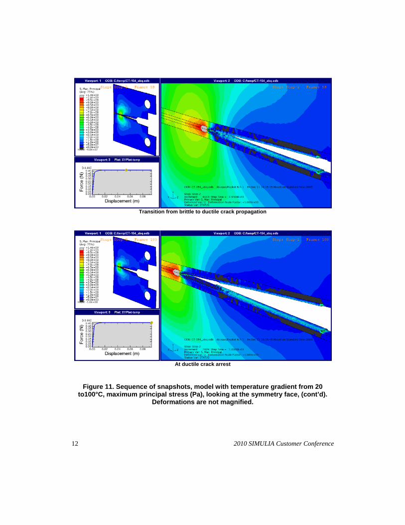
Transition from brittle to ductile crack propagation

At ductile crack arrest

Figure 11. Sequence of snapshots, model with temperature gradient from 20 to100°C, maximum principal stress (Pa), looking at the symmetry face, (cont’d).

Deformations are not magnified.

2010 SIMULIA Customer Conference 13

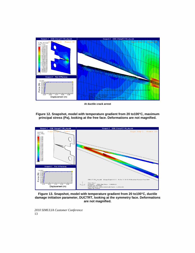
At ductile crack arrest

Figure 12. Snapshot, model with temperature gradient from 20 to100°C, maximum principal stress (Pa), looking at the free face. Deformations are not magnified.

Figure 13. Snapshot, model with temperature gradient from 20 to100°C, ductile

damage initiation parameter, DUCTRT, looking at the symmetry face. Deformations are not magnified.

14 2010 SIMULIA Customer Conference

8. Conclusions

A methodology to simulate brittle crack initiation, followed by brittle or ductile propagation and brittle or ductile crack arrest was developed. Two material models, the Bao-Wierzbicki ductile failure criteria and cohesive contact, were used in this methodology. Parameters for the material models were calibrated by matching simulated toughness results and experimental results. Successful analyses demonstrated that this methodology can simulate brittle crack initiation, followed by brittle or ductile propagation and brittle or ductile crack arrest. The following topics were suggested for investigation, in order to further develop this methodology:

• Studying dynamic effects and the impact of the duration of load application. • Investigating the sensitivity of the results to crack propagation velocities. • Quantifying mesh sensitivity. • Validation of FEM against crack arrest experiments.

9. References

1. ASTM International. (2001) “ASTM E1820-01, Standard Test Method for Measurement of Fracture Toughness” Annual Book of ASTM Standards, Vol 03.01.

2. ASTM International. (2005) “ASTM E1921-05, Standard Test Method for Determination of Reference Temperature, T0, for Ferritic Steels in the Transition Range” Annual Book of ASTM Standards

3. Chaouadi, R. and Fabry, A. (2002). “On the Utilization of the Instrumented Charpy Impact Test.” From Charpy to Present Impact Testing ESIS Publication 30. eds. François, D., Pineau, A. Elsevier p.107

4. Haggag, F. M., Wang, J. A., and Theiss, T. J., Using Portable/In-Situ Stress-Strain Microprobe System to Measure Mechanical Properties of Steel Bridges During Service. Advanced Technology Corp., http://www.atc-ssm.com/pdf/SPIE2946.pdf

5. Hiser, A. L., (1990). Correlation for Irradiation-Induced Transition Temperature Increases From Cv ad KJC and KIC

6. Hiser, A. L. (1993). “Specimen Size Effects on J-R Curves for RPV Steels.” Constraint Effects in Fracture. ASTM STP 1171, eds. Hackett, E.M., Schwalbe, K.-H, and Dodds, R.H. p. 195-238

Data, Final Report. NUREG/CR-5494, MEA-2377, RF, R5. prepared for Division of Engineering, Office of nuclear regulatory research, US. Nuclear Regulatory Commission

7. Jeong, D.Y., Yu, H., Gordon, J.E., Tang, Y.H. Finite Element Analysis of Unnotched Charpy Impact Tests. U.S. Department of Transportation. Volpe National Transportation Systems Center, Cambridge, Massachusetts, USA

8. Tanguy, B., Besson, J., Piques, R., Pineau, A. (2005). “Ductile to Brittle Transition of an A508 Steel Characterized by Charpy Impact Test, Part II: Modeling of the Charpy Transition Curve.” Engineering Fracture Mechanics 72, 413–434

2010 SIMULIA Customer Conference 15

9. Wallin, K. (2001). “Correlation Between Static Initiation Toughness KJc and Crack Arrest Toughness KIa 2024-T351 Aluminum Alloy.” Fatigue and Fracture Mechanics: 32nd Volume ASTM STP 1406, Chona, R. Ed., American Society for Testing and Materials, 17-34