Rethinking Natural Image Priors

Yair Weiss

Hebrew University of Jerusalem

Outline

• “Position part” — relation between BV and CV.• “Research part” — image priors paper (ICCV 11). Joint

work with Daniel Zoran.

Relationship

• Biological and Human Vision.• Machine Vision

Relationship

• Biological and Human Vision.• Visual World• Machine Vision

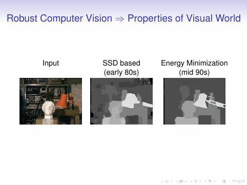
Robust Computer Vision⇒ Properties of Visual World

Input SSD based Energy Minimization(early 80s) (mid 90s)

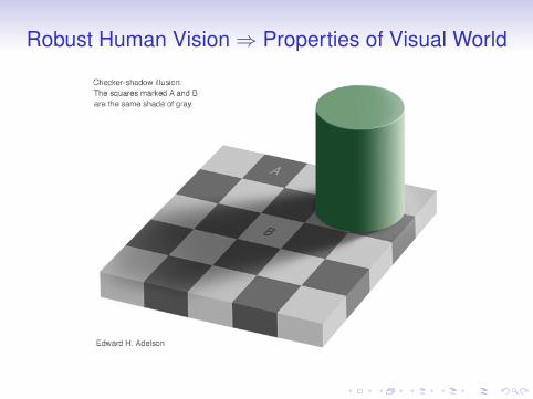
Robust Human Vision⇒ Properties of Visual World

Relationship

• Biological and Human Vision.• Visual World• Machine Vision

Natural Image Priors

Given a N × N matrix x , return Pr(x) “Probability that x is anatural image”.

Motivation:

Given a N ! N matrix x, return Pr(x) “Probability that x is a

natural image”. .

likely less likely really unlikely

Zhu and Mumford, Portilla and Simoncelli, Roth and Black, Weiss andFreeman, Osindero, Welling and Hinton, Ranzato and Lecun,Olshausen, Lewicki, Ng, Aharon and Elad, Mairal, Sapiro, · · ·

Biological Vison⇔ Computer Vision

Prior based methods vs. Prior Free methods

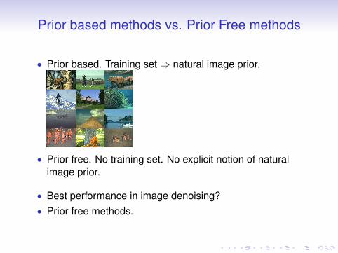
• Prior based. Training set⇒ natural image prior.

Roth and Black 2005

Training Images Filter Set

? ? ? ? ?? ? ? ? ?? ? ? ? ?? ? ? ? ?? ? ? ? ?

Pr(x; filters, energy) =1

Ze!E(x)

Maximum Likelihood "Filters Energy

???!1 !0.5 0 0.5 1

100

response

energy

• Prior free. No training set. No explicit notion of naturalimage prior.

• Best performance in image denoising?

• Prior free methods.

Prior based methods vs. Prior Free methods

• Prior based. Training set⇒ natural image prior.

Roth and Black 2005

Training Images Filter Set

? ? ? ? ?? ? ? ? ?? ? ? ? ?? ? ? ? ?? ? ? ? ?

Pr(x; filters, energy) =1

Ze!E(x)

Maximum Likelihood "Filters Energy

???!1 !0.5 0 0.5 1

100

response

energy

• Prior free. No training set. No explicit notion of naturalimage prior.

• Best performance in image denoising?• Prior free methods.

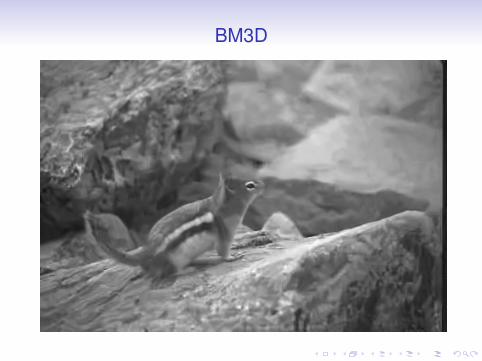
The BM3D Prior free method

!"#$ %$ &''()*+,*"-. -/ *01 23) 4)0-5. -. *01 +"#0* )"617 ,/*1+ *+"88".# /-+ /-(+ 9,+*":(',+ ,6,9*";1<)0,91 .1"#0=-+0--6)$ >01 #+11. -;1+',? ") ()16 *- )0-5*01 /-(.6 )"8"',+ .1"#0=-+0--6) ()16 *- /-+8 , @<A #+-(9$ >01 23) ,+1 '")*16 ". 61:+1,)".# 8,#."*(61 -/ *01"+ :-++1)9-.6".# 1"#1.;,'(1)$ B.1 :,. -=)1+;1*0,* *01 !+)* /15 23) 0,;1 *01 )*+-.#1)* )"8"',+"*? 5"*0 *01 .-")1</+11 )"#.,' ". *01 .1"#0=-+0--6$

Buades et al. 05, Dabov et al. 06, Elad et a. 07,Mairal et al. 10, Liuand Simoncelli 08

Comparison

100 different test images.• BM3D vs. Fields of Expert (Roth and Black)

• BM3D is better 100/100 times.• BM3D vs. generic KSVD (Elad and Aharon)• BM3D is better 89/100 times.

Comparison

100 different test images.• BM3D vs. Fields of Expert (Roth and Black)• BM3D is better 100/100 times.

• BM3D vs. generic KSVD (Elad and Aharon)• BM3D is better 89/100 times.

Comparison

100 different test images.• BM3D vs. Fields of Expert (Roth and Black)• BM3D is better 100/100 times.• BM3D vs. generic KSVD (Elad and Aharon)

• BM3D is better 89/100 times.

Comparison

100 different test images.• BM3D vs. Fields of Expert (Roth and Black)• BM3D is better 100/100 times.• BM3D vs. generic KSVD (Elad and Aharon)• BM3D is better 89/100 times.

Noisy

FOE

BM3D

What’s going on?

Roth and Black 2005

Training Images Filter Set

? ? ? ? ?? ? ? ? ?? ? ? ? ?? ? ? ? ?? ? ? ? ?

Pr(x; filters, energy) =1

Ze!E(x)

Maximum Likelihood "Filters Energy

???!1 !0.5 0 0.5 1

100

response

energy

• “generic natural image” — too general?• Training using maximum likelihood the wrong thing?

• Current prior models poor (even in the likelihood sense).

What’s going on?

Roth and Black 2005

Training Images Filter Set

? ? ? ? ?? ? ? ? ?? ? ? ? ?? ? ? ? ?? ? ? ? ?

Pr(x; filters, energy) =1

Ze!E(x)

Maximum Likelihood "Filters Energy

???!1 !0.5 0 0.5 1

100

response

energy

• “generic natural image” — too general?• Training using maximum likelihood the wrong thing?• Current prior models poor (even in the likelihood sense).

What’s going oncan be learned either from a set of natural image patches(generic, or global as it is sometimes called) or the noisyimage itself (image based). Using this dictionary, all overlap-ping patches of the image are denoised independently andthen averaged to obtain a new reconstructed image. Thisprocess is repeated for several iterations using this new esti-mated image. Learning the dictionary in KSVD is differentthan learning a patch prior because it may be performedas part of the optimization process (unless the dictionaryis learned beforehand from natural images), but the opti-mization in KSVD can be seen as a special case of ourmethod - when the prior is a sparse prior, our cost functionand KSVD’s are the same. We note again, however, thatour framework allows for much richer priors which can belearned beforehand over patches - as we will see later on,this boasts some tremendous benefits.

A whole family of patch based methods [2, 5, 8] use thenoisy image itself in order to denoise. These “non-local”methods look for similarities within the noisy image itselfand operate on these similar patches together. BM3D [5]groups together similar patches into “blocks”, transformsthem into wavelet coefficients (in all 3 dimensions), thresh-olds and transforms backs, using all the estimates together.Mairal et al. [8] which is currently state-of-the-art take a sim-ilar approach to this, but instead of transforming the patchesvia a wavelet transform, sparse coding using a learned dic-tionary is used, where each block is constrained to use thesame dictionary elements. One thing which is common to allof the above non-local methods, and indeed almost all patchbased methods, is that they all average the clean patchestogether to form the final estimate of the image. As we haveseen in Section 3, this may not be the optimal thing to do.

3.3. Patch Likelihoods and the EPLL Framework

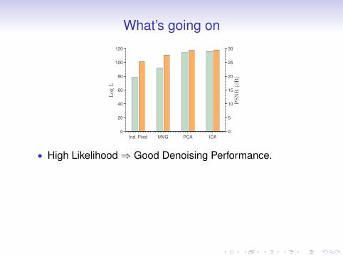
We have seen that the EPLL cost function (Equation2) depends on the likelihood of patches. Going back tothe priors from Section 2 we now ask - do better priors(in the likelihood sense) also lead to better whole imagedenoising with the proposed EPLL framework? Figure 4shows the average PSNR obtained with 5 different imagesfrom the Berkeley training set, corrupted with Gaussiannoise at ! = 25 and denoised using each of the priors insection 2. We compare the result obtained using simple patchaveraging (PA) and our proposed EPLL framework. It can beseen that indeed - better likelihood on patches leads to betterdenoising both on independent patches (Figure 1) and wholeimages (Figure 4). Additionally, it can be seen that EPLLimproves denoising results significantly when compared tosimple patch averaging (Figure 4).

These results motivate the question: Can we find a betterprior for image patches?

Ind. Pixel MVG PCA ICA

0

20

40

60

80

100

120

Log

L

0

5

10

15

20

25

30

PSN

R(d

B)

(a)Ind. Pixel MVG PCA ICA

25

26

27

28

29

30

Patch Average

EPLL

(b)

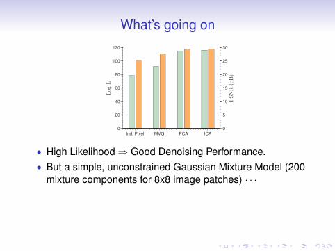
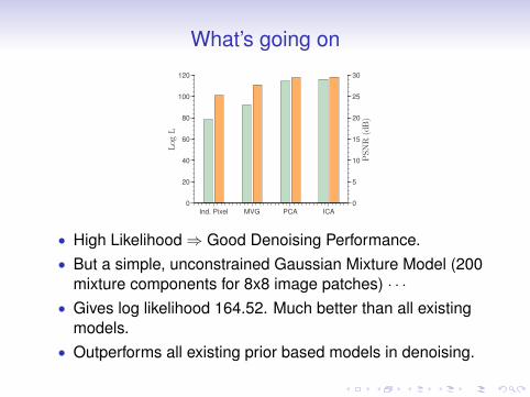
Figure 4: (a) Whole image denoising with the proposed frameworkwith all the priors discussed in Section 2. It can be seen that betterpriors (in the likelihood sense) lead to better denoising performanceon whole images, left bar is log L, right bar is PSNR. (b) Note howthe EPLL framework improves performance significantly whencompared to simple patch averaging (PA)

4. Can We Learn Better Patch Priors?In addition to the priors discussed in Section 2 we intro-

duce a new, simple yet surprisingly rich prior.

4.1. Learning and Inference with a Gaussian Mix-ture Prior

We learn a finite Gaussian mixture model over the pixelsof natural image patches. Many popular image priors canbe seen as special cases of a GMM (e.g. [9, 1, 14]) butthey typically constrain the means and covariance matricesduring learning. In contrast, we do not constrain the model inany way — we learn the means, full covariance matrices andmixing weights, over all pixels. Learning is easily performedusing the Expectation Maximization algorithm (EM). Withthis model, calculating the log likelihood of a given patch istrivial:

log p(x) = log

!K"

k=1

"kN(x|µk, !k)

#(5)

Where "k are the mixing weights for each of the mixturecomponent and µk and !k are the corresponding mean andcovariance matrix.

Given a noisy patch y, the BLS estimate can be calcu-lated in closed form (as the posterior is just another Gaussianmixture) [1]. The MAP estimate, however, can not be cal-culated in closed form. To tackle this we use the followingapproximate MAP estimation procedure:

1. Given noisy patch y we calculate the conditional mix-ing weights "!k = P (k|y).

2. We choose the component which has the highest condi-tional mixing weight kmax = maxk "!k.

3. The MAP estimate x̂ is then a Wiener filter solution forthe kmax-th component:

x̂ =$!kmax

+ !2I%"1 $

!kmaxy + !2Iµkmax

%

• High Likelihood⇒ Good Denoising Performance.

• But a simple, unconstrained Gaussian Mixture Model (200mixture components for 8x8 image patches) · · ·

• Gives log likelihood 164.52. Much better than all existingmodels.

• Outperforms all existing prior based models in denoising.

What’s going oncan be learned either from a set of natural image patches(generic, or global as it is sometimes called) or the noisyimage itself (image based). Using this dictionary, all overlap-ping patches of the image are denoised independently andthen averaged to obtain a new reconstructed image. Thisprocess is repeated for several iterations using this new esti-mated image. Learning the dictionary in KSVD is differentthan learning a patch prior because it may be performedas part of the optimization process (unless the dictionaryis learned beforehand from natural images), but the opti-mization in KSVD can be seen as a special case of ourmethod - when the prior is a sparse prior, our cost functionand KSVD’s are the same. We note again, however, thatour framework allows for much richer priors which can belearned beforehand over patches - as we will see later on,this boasts some tremendous benefits.

A whole family of patch based methods [2, 5, 8] use thenoisy image itself in order to denoise. These “non-local”methods look for similarities within the noisy image itselfand operate on these similar patches together. BM3D [5]groups together similar patches into “blocks”, transformsthem into wavelet coefficients (in all 3 dimensions), thresh-olds and transforms backs, using all the estimates together.Mairal et al. [8] which is currently state-of-the-art take a sim-ilar approach to this, but instead of transforming the patchesvia a wavelet transform, sparse coding using a learned dic-tionary is used, where each block is constrained to use thesame dictionary elements. One thing which is common to allof the above non-local methods, and indeed almost all patchbased methods, is that they all average the clean patchestogether to form the final estimate of the image. As we haveseen in Section 3, this may not be the optimal thing to do.

3.3. Patch Likelihoods and the EPLL Framework

We have seen that the EPLL cost function (Equation2) depends on the likelihood of patches. Going back tothe priors from Section 2 we now ask - do better priors(in the likelihood sense) also lead to better whole imagedenoising with the proposed EPLL framework? Figure 4shows the average PSNR obtained with 5 different imagesfrom the Berkeley training set, corrupted with Gaussiannoise at ! = 25 and denoised using each of the priors insection 2. We compare the result obtained using simple patchaveraging (PA) and our proposed EPLL framework. It can beseen that indeed - better likelihood on patches leads to betterdenoising both on independent patches (Figure 1) and wholeimages (Figure 4). Additionally, it can be seen that EPLLimproves denoising results significantly when compared tosimple patch averaging (Figure 4).

These results motivate the question: Can we find a betterprior for image patches?

Ind. Pixel MVG PCA ICA

0

20

40

60

80

100

120

Log

L

0

5

10

15

20

25

30

PSN

R(d

B)

(a)Ind. Pixel MVG PCA ICA

25

26

27

28

29

30

Patch Average

EPLL

(b)

Figure 4: (a) Whole image denoising with the proposed frameworkwith all the priors discussed in Section 2. It can be seen that betterpriors (in the likelihood sense) lead to better denoising performanceon whole images, left bar is log L, right bar is PSNR. (b) Note howthe EPLL framework improves performance significantly whencompared to simple patch averaging (PA)

4. Can We Learn Better Patch Priors?In addition to the priors discussed in Section 2 we intro-

duce a new, simple yet surprisingly rich prior.

4.1. Learning and Inference with a Gaussian Mix-ture Prior

We learn a finite Gaussian mixture model over the pixelsof natural image patches. Many popular image priors canbe seen as special cases of a GMM (e.g. [9, 1, 14]) butthey typically constrain the means and covariance matricesduring learning. In contrast, we do not constrain the model inany way — we learn the means, full covariance matrices andmixing weights, over all pixels. Learning is easily performedusing the Expectation Maximization algorithm (EM). Withthis model, calculating the log likelihood of a given patch istrivial:

log p(x) = log

!K"

k=1

"kN(x|µk, !k)

#(5)

Where "k are the mixing weights for each of the mixturecomponent and µk and !k are the corresponding mean andcovariance matrix.

Given a noisy patch y, the BLS estimate can be calcu-lated in closed form (as the posterior is just another Gaussianmixture) [1]. The MAP estimate, however, can not be cal-culated in closed form. To tackle this we use the followingapproximate MAP estimation procedure:

1. Given noisy patch y we calculate the conditional mix-ing weights "!k = P (k|y).

2. We choose the component which has the highest condi-tional mixing weight kmax = maxk "!k.

3. The MAP estimate x̂ is then a Wiener filter solution forthe kmax-th component:

x̂ =$!kmax

+ !2I%"1 $

!kmaxy + !2Iµkmax

%

• High Likelihood⇒ Good Denoising Performance.• But a simple, unconstrained Gaussian Mixture Model (200

mixture components for 8x8 image patches) · · ·

• Gives log likelihood 164.52. Much better than all existingmodels.

• Outperforms all existing prior based models in denoising.

What’s going oncan be learned either from a set of natural image patches(generic, or global as it is sometimes called) or the noisyimage itself (image based). Using this dictionary, all overlap-ping patches of the image are denoised independently andthen averaged to obtain a new reconstructed image. Thisprocess is repeated for several iterations using this new esti-mated image. Learning the dictionary in KSVD is differentthan learning a patch prior because it may be performedas part of the optimization process (unless the dictionaryis learned beforehand from natural images), but the opti-mization in KSVD can be seen as a special case of ourmethod - when the prior is a sparse prior, our cost functionand KSVD’s are the same. We note again, however, thatour framework allows for much richer priors which can belearned beforehand over patches - as we will see later on,this boasts some tremendous benefits.

A whole family of patch based methods [2, 5, 8] use thenoisy image itself in order to denoise. These “non-local”methods look for similarities within the noisy image itselfand operate on these similar patches together. BM3D [5]groups together similar patches into “blocks”, transformsthem into wavelet coefficients (in all 3 dimensions), thresh-olds and transforms backs, using all the estimates together.Mairal et al. [8] which is currently state-of-the-art take a sim-ilar approach to this, but instead of transforming the patchesvia a wavelet transform, sparse coding using a learned dic-tionary is used, where each block is constrained to use thesame dictionary elements. One thing which is common to allof the above non-local methods, and indeed almost all patchbased methods, is that they all average the clean patchestogether to form the final estimate of the image. As we haveseen in Section 3, this may not be the optimal thing to do.

3.3. Patch Likelihoods and the EPLL Framework

We have seen that the EPLL cost function (Equation2) depends on the likelihood of patches. Going back tothe priors from Section 2 we now ask - do better priors(in the likelihood sense) also lead to better whole imagedenoising with the proposed EPLL framework? Figure 4shows the average PSNR obtained with 5 different imagesfrom the Berkeley training set, corrupted with Gaussiannoise at ! = 25 and denoised using each of the priors insection 2. We compare the result obtained using simple patchaveraging (PA) and our proposed EPLL framework. It can beseen that indeed - better likelihood on patches leads to betterdenoising both on independent patches (Figure 1) and wholeimages (Figure 4). Additionally, it can be seen that EPLLimproves denoising results significantly when compared tosimple patch averaging (Figure 4).

These results motivate the question: Can we find a betterprior for image patches?

Ind. Pixel MVG PCA ICA

0

20

40

60

80

100

120

Log

L

0

5

10

15

20

25

30

PSN

R(d

B)

(a)Ind. Pixel MVG PCA ICA

25

26

27

28

29

30

Patch Average

EPLL

(b)

Figure 4: (a) Whole image denoising with the proposed frameworkwith all the priors discussed in Section 2. It can be seen that betterpriors (in the likelihood sense) lead to better denoising performanceon whole images, left bar is log L, right bar is PSNR. (b) Note howthe EPLL framework improves performance significantly whencompared to simple patch averaging (PA)

4. Can We Learn Better Patch Priors?In addition to the priors discussed in Section 2 we intro-

duce a new, simple yet surprisingly rich prior.

4.1. Learning and Inference with a Gaussian Mix-ture Prior

We learn a finite Gaussian mixture model over the pixelsof natural image patches. Many popular image priors canbe seen as special cases of a GMM (e.g. [9, 1, 14]) butthey typically constrain the means and covariance matricesduring learning. In contrast, we do not constrain the model inany way — we learn the means, full covariance matrices andmixing weights, over all pixels. Learning is easily performedusing the Expectation Maximization algorithm (EM). Withthis model, calculating the log likelihood of a given patch istrivial:

log p(x) = log

!K"

k=1

"kN(x|µk, !k)

#(5)

Where "k are the mixing weights for each of the mixturecomponent and µk and !k are the corresponding mean andcovariance matrix.

Given a noisy patch y, the BLS estimate can be calcu-lated in closed form (as the posterior is just another Gaussianmixture) [1]. The MAP estimate, however, can not be cal-culated in closed form. To tackle this we use the followingapproximate MAP estimation procedure:

1. Given noisy patch y we calculate the conditional mix-ing weights "!k = P (k|y).

2. We choose the component which has the highest condi-tional mixing weight kmax = maxk "!k.

3. The MAP estimate x̂ is then a Wiener filter solution forthe kmax-th component:

x̂ =$!kmax

+ !2I%"1 $

!kmaxy + !2Iµkmax

%

• High Likelihood⇒ Good Denoising Performance.• But a simple, unconstrained Gaussian Mixture Model (200

mixture components for 8x8 image patches) · · ·• Gives log likelihood 164.52. Much better than all existing

models.• Outperforms all existing prior based models in denoising.

Noisy

FOE

GMM

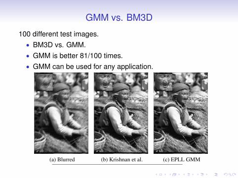
GMM vs. BM3D

100 different test images.• BM3D vs. GMM.

• GMM is better 81/100 times.• GMM can be used for any application.

(a) Blurred (b) Krishnan et al. (c) EPLL GMM

Krishnan et al. EPLL-GMM

Kernel 1 17! 17 25.84 27.17

Kernel 2 19! 19 26.38 27.70

Figure 8: Deblurring experiments

5. DiscussionPatch based models are easier to learn and to work with

than whole image models. We have shown that patch modelswhich give high likelihood values for patches sampled fromnatural images perform better in patch and image restora-tion tasks. Given these results, we have proposed a frame-work which allows the use of patch models for whole imagerestoration, motivated by the idea that patches in the restoredimage should be likely under the prior. We have shown thatthis framework improves the results of whole image restora-tion considerably when compared to simple patch averaging,used by most present day methods. Finally, we have pro-posed a new, simple yet rich Gaussian Mixture prior whichperforms surprisingly well on image denoising, deblurringand inpainting.

While we have demonstrated our framework using only afew priors, one of its greater strengths is the fact that it canserve as a “plug-in” system - it can work with any existingpatch restoration method. Considering the fact that bothBM3D and LLSC are patch based methods which use simplepatch averaging, it would be interesting to see how wouldthese methods benefit from the proposed framework.

Finally, perhaps the most surprising result of this work,and the direction in which much is left to be explored, is thestellar performance of the GMM model. The GMM modelused here is extremely naive - a simple mixture of Gaussianswith full covariance matrices. Given the fact that GaussianMixtures are an extremely studied area, incorporating moresophisticated machinery into the learning and the represen-tation of this model holds much promise - and this is ourcurrent line of research.

Acknowledgments

The authors wish to thank Anat Levin for helpful discussions.

References[1] J. Portilla, V. Strela, M. Wainwright, and E. Simoncelli, “Im-

age denoising using scale mixtures of gaussians in the waveletdomain,” IEEE Transactions on Image Processing, vol. 12,no. 11, pp. 1338–1351, 2003.

[2] A. Buades, B. Coll, and J. Morel, “A non-local algorithm forimage denoising,” in Computer Vision and Pattern Recogni-tion, 2005. CVPR 2005. IEEE Computer Society Conferenceon, vol. 2, pp. 60–65, IEEE, 2005.

[3] M. Elad and M. Aharon, “Image denoising via sparse andredundant representations over learned dictionaries,” ImageProcessing, IEEE Transactions on, vol. 15, no. 12, pp. 3736–3745, 2006.

[4] Y. Hel-Or and D. Shaked, “A discriminative approach forwavelet denoising,” IEEE Transactions on Image Processing,vol. 17, no. 4, p. 443, 2008.

[5] K. Dabov, A. Foi, V. Katkovnik, and K. Egiazarian, “Im-age restoration by sparse 3D transform-domain collaborativefiltering,” in SPIE Electronic Imaging, 2008.

[6] S. Roth and M. Black, “Fields of experts,” International Jour-nal of Computer Vision, vol. 82, no. 2, pp. 205–229, 2009.

[7] D. Krishnan and R. Fergus, “Fast image deconvolution usinghyper-laplacian priors,” in Advances in Neural InformationProcessing Systems 22, pp. 1033–1041, 2009.

[8] J. Mairal, F. Bach, J. Ponce, G. Sapiro, and A. Zisserman,“Non-local sparse models for image restoration,” in Com-puter Vision, 2009 IEEE 12th International Conference on,pp. 2272–2279, IEEE, 2010.

[9] Y. Weiss and W. Freeman, “What makes a good model ofnatural images?,” CVPR ’07. IEEE Conference on, pp. 1–8,June 2007.

[10] D. Martin, C. Fowlkes, D. Tal, and J. Malik, “A databaseof human segmented natural images and its application toevaluating segmentation algorithms and measuring ecologicalstatistics,” in Proc. 8th Int’l Conf. Computer Vision, vol. 2,pp. 416–423, July 2001.

[11] D. Geman and C. Yang, “Nonlinear image recovery withhalf-quadratic regularization,” Image Processing, IEEE Trans-actions on, vol. 4, no. 7, pp. 932–946, 2002.

[12] D. Zoran and Y. Weiss, “Scale invariance and noise in naturalimages,” in Computer Vision, 2009 IEEE 12th InternationalConference on, pp. 2209–2216, Citeseer, 2009.

[13] B. Lindsay, “Composite likelihood methods,” ContemporaryMathematics, vol. 80, no. 1, pp. 221–39, 1988.

[14] J. Domke, A. Karapurkar, and Y. Aloimonos, “Who killedthe directed model?,” in CVPR 2008. IEEE Conference on,pp. 1–8, IEEE, 2008.

[15] M. Carreira-Perpiñán, “Mode-finding for mixtures of Gaus-sian distributions,” Pattern Analysis and Machine Intelligence,IEEE Transactions on, vol. 22, no. 11, pp. 1318–1323, 2002.

[16] G. Yu, G. Sapiro, and S. Mallat, “Solving inverse problemswith piecewise linear estimators: From gaussian mixture mod-els to structured sparsity,” CoRR, vol. abs/1006.3056, 2010.

GMM vs. BM3D

100 different test images.• BM3D vs. GMM.• GMM is better 81/100 times.

• GMM can be used for any application.

(a) Blurred (b) Krishnan et al. (c) EPLL GMM

Krishnan et al. EPLL-GMM

Kernel 1 17! 17 25.84 27.17

Kernel 2 19! 19 26.38 27.70

Figure 8: Deblurring experiments

5. DiscussionPatch based models are easier to learn and to work with

than whole image models. We have shown that patch modelswhich give high likelihood values for patches sampled fromnatural images perform better in patch and image restora-tion tasks. Given these results, we have proposed a frame-work which allows the use of patch models for whole imagerestoration, motivated by the idea that patches in the restoredimage should be likely under the prior. We have shown thatthis framework improves the results of whole image restora-tion considerably when compared to simple patch averaging,used by most present day methods. Finally, we have pro-posed a new, simple yet rich Gaussian Mixture prior whichperforms surprisingly well on image denoising, deblurringand inpainting.

While we have demonstrated our framework using only afew priors, one of its greater strengths is the fact that it canserve as a “plug-in” system - it can work with any existingpatch restoration method. Considering the fact that bothBM3D and LLSC are patch based methods which use simplepatch averaging, it would be interesting to see how wouldthese methods benefit from the proposed framework.

Finally, perhaps the most surprising result of this work,and the direction in which much is left to be explored, is thestellar performance of the GMM model. The GMM modelused here is extremely naive - a simple mixture of Gaussianswith full covariance matrices. Given the fact that GaussianMixtures are an extremely studied area, incorporating moresophisticated machinery into the learning and the represen-tation of this model holds much promise - and this is ourcurrent line of research.

Acknowledgments

The authors wish to thank Anat Levin for helpful discussions.

References[1] J. Portilla, V. Strela, M. Wainwright, and E. Simoncelli, “Im-

age denoising using scale mixtures of gaussians in the waveletdomain,” IEEE Transactions on Image Processing, vol. 12,no. 11, pp. 1338–1351, 2003.

[2] A. Buades, B. Coll, and J. Morel, “A non-local algorithm forimage denoising,” in Computer Vision and Pattern Recogni-tion, 2005. CVPR 2005. IEEE Computer Society Conferenceon, vol. 2, pp. 60–65, IEEE, 2005.

[3] M. Elad and M. Aharon, “Image denoising via sparse andredundant representations over learned dictionaries,” ImageProcessing, IEEE Transactions on, vol. 15, no. 12, pp. 3736–3745, 2006.

[4] Y. Hel-Or and D. Shaked, “A discriminative approach forwavelet denoising,” IEEE Transactions on Image Processing,vol. 17, no. 4, p. 443, 2008.

[5] K. Dabov, A. Foi, V. Katkovnik, and K. Egiazarian, “Im-age restoration by sparse 3D transform-domain collaborativefiltering,” in SPIE Electronic Imaging, 2008.

[6] S. Roth and M. Black, “Fields of experts,” International Jour-nal of Computer Vision, vol. 82, no. 2, pp. 205–229, 2009.

[7] D. Krishnan and R. Fergus, “Fast image deconvolution usinghyper-laplacian priors,” in Advances in Neural InformationProcessing Systems 22, pp. 1033–1041, 2009.

[8] J. Mairal, F. Bach, J. Ponce, G. Sapiro, and A. Zisserman,“Non-local sparse models for image restoration,” in Com-puter Vision, 2009 IEEE 12th International Conference on,pp. 2272–2279, IEEE, 2010.

[9] Y. Weiss and W. Freeman, “What makes a good model ofnatural images?,” CVPR ’07. IEEE Conference on, pp. 1–8,June 2007.

[10] D. Martin, C. Fowlkes, D. Tal, and J. Malik, “A databaseof human segmented natural images and its application toevaluating segmentation algorithms and measuring ecologicalstatistics,” in Proc. 8th Int’l Conf. Computer Vision, vol. 2,pp. 416–423, July 2001.

[11] D. Geman and C. Yang, “Nonlinear image recovery withhalf-quadratic regularization,” Image Processing, IEEE Trans-actions on, vol. 4, no. 7, pp. 932–946, 2002.

[12] D. Zoran and Y. Weiss, “Scale invariance and noise in naturalimages,” in Computer Vision, 2009 IEEE 12th InternationalConference on, pp. 2209–2216, Citeseer, 2009.

[13] B. Lindsay, “Composite likelihood methods,” ContemporaryMathematics, vol. 80, no. 1, pp. 221–39, 1988.

[14] J. Domke, A. Karapurkar, and Y. Aloimonos, “Who killedthe directed model?,” in CVPR 2008. IEEE Conference on,pp. 1–8, IEEE, 2008.

[15] M. Carreira-Perpiñán, “Mode-finding for mixtures of Gaus-sian distributions,” Pattern Analysis and Machine Intelligence,IEEE Transactions on, vol. 22, no. 11, pp. 1318–1323, 2002.

[16] G. Yu, G. Sapiro, and S. Mallat, “Solving inverse problemswith piecewise linear estimators: From gaussian mixture mod-els to structured sparsity,” CoRR, vol. abs/1006.3056, 2010.

GMM vs. BM3D

100 different test images.• BM3D vs. GMM.• GMM is better 81/100 times.• GMM can be used for any application.

(a) Blurred (b) Krishnan et al. (c) EPLL GMM

Krishnan et al. EPLL-GMM

Kernel 1 17! 17 25.84 27.17

Kernel 2 19! 19 26.38 27.70

Figure 8: Deblurring experiments

5. DiscussionPatch based models are easier to learn and to work with

than whole image models. We have shown that patch modelswhich give high likelihood values for patches sampled fromnatural images perform better in patch and image restora-tion tasks. Given these results, we have proposed a frame-work which allows the use of patch models for whole imagerestoration, motivated by the idea that patches in the restoredimage should be likely under the prior. We have shown thatthis framework improves the results of whole image restora-tion considerably when compared to simple patch averaging,used by most present day methods. Finally, we have pro-posed a new, simple yet rich Gaussian Mixture prior whichperforms surprisingly well on image denoising, deblurringand inpainting.

While we have demonstrated our framework using only afew priors, one of its greater strengths is the fact that it canserve as a “plug-in” system - it can work with any existingpatch restoration method. Considering the fact that bothBM3D and LLSC are patch based methods which use simplepatch averaging, it would be interesting to see how wouldthese methods benefit from the proposed framework.

Finally, perhaps the most surprising result of this work,and the direction in which much is left to be explored, is thestellar performance of the GMM model. The GMM modelused here is extremely naive - a simple mixture of Gaussianswith full covariance matrices. Given the fact that GaussianMixtures are an extremely studied area, incorporating moresophisticated machinery into the learning and the represen-tation of this model holds much promise - and this is ourcurrent line of research.

Acknowledgments

The authors wish to thank Anat Levin for helpful discussions.

References[1] J. Portilla, V. Strela, M. Wainwright, and E. Simoncelli, “Im-

age denoising using scale mixtures of gaussians in the waveletdomain,” IEEE Transactions on Image Processing, vol. 12,no. 11, pp. 1338–1351, 2003.

[2] A. Buades, B. Coll, and J. Morel, “A non-local algorithm forimage denoising,” in Computer Vision and Pattern Recogni-tion, 2005. CVPR 2005. IEEE Computer Society Conferenceon, vol. 2, pp. 60–65, IEEE, 2005.

[3] M. Elad and M. Aharon, “Image denoising via sparse andredundant representations over learned dictionaries,” ImageProcessing, IEEE Transactions on, vol. 15, no. 12, pp. 3736–3745, 2006.

[4] Y. Hel-Or and D. Shaked, “A discriminative approach forwavelet denoising,” IEEE Transactions on Image Processing,vol. 17, no. 4, p. 443, 2008.

[5] K. Dabov, A. Foi, V. Katkovnik, and K. Egiazarian, “Im-age restoration by sparse 3D transform-domain collaborativefiltering,” in SPIE Electronic Imaging, 2008.

[6] S. Roth and M. Black, “Fields of experts,” International Jour-nal of Computer Vision, vol. 82, no. 2, pp. 205–229, 2009.

[7] D. Krishnan and R. Fergus, “Fast image deconvolution usinghyper-laplacian priors,” in Advances in Neural InformationProcessing Systems 22, pp. 1033–1041, 2009.

[8] J. Mairal, F. Bach, J. Ponce, G. Sapiro, and A. Zisserman,“Non-local sparse models for image restoration,” in Com-puter Vision, 2009 IEEE 12th International Conference on,pp. 2272–2279, IEEE, 2010.

[9] Y. Weiss and W. Freeman, “What makes a good model ofnatural images?,” CVPR ’07. IEEE Conference on, pp. 1–8,June 2007.

[10] D. Martin, C. Fowlkes, D. Tal, and J. Malik, “A databaseof human segmented natural images and its application toevaluating segmentation algorithms and measuring ecologicalstatistics,” in Proc. 8th Int’l Conf. Computer Vision, vol. 2,pp. 416–423, July 2001.

[11] D. Geman and C. Yang, “Nonlinear image recovery withhalf-quadratic regularization,” Image Processing, IEEE Trans-actions on, vol. 4, no. 7, pp. 932–946, 2002.

[12] D. Zoran and Y. Weiss, “Scale invariance and noise in naturalimages,” in Computer Vision, 2009 IEEE 12th InternationalConference on, pp. 2209–2216, Citeseer, 2009.

[13] B. Lindsay, “Composite likelihood methods,” ContemporaryMathematics, vol. 80, no. 1, pp. 221–39, 1988.

[14] J. Domke, A. Karapurkar, and Y. Aloimonos, “Who killedthe directed model?,” in CVPR 2008. IEEE Conference on,pp. 1–8, IEEE, 2008.

[15] M. Carreira-Perpiñán, “Mode-finding for mixtures of Gaus-sian distributions,” Pattern Analysis and Machine Intelligence,IEEE Transactions on, vol. 22, no. 11, pp. 1318–1323, 2002.

[16] G. Yu, G. Sapiro, and S. Mallat, “Solving inverse problemswith piecewise linear estimators: From gaussian mixture mod-els to structured sparsity,” CoRR, vol. abs/1006.3056, 2010.

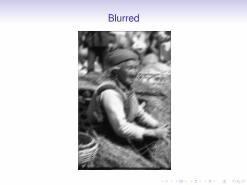
Blurred

Sparse Derivative

GMM

Secret of GMM

! KSVDG FoE GMM-EPLL

15 30.67 30.18 31.2125 28.28 27.77 28.7150 25.18 23.29 25.72

100 22.39 16.68 23.19

(a) Generic Priors

! KSVD BM3D LLSC GMM-EPLL

15 30.59 30.87 31.27 31.21

25 28.20 28.57 28.70 28.7150 25.15 25.63 25.73 25.72

100 22.40 23.25 23.15 23.19

(b) Image Based Methods

Table 2: Summary of denoising experiments results. Our method is clearly state-of-the-art when compared to generic priors, and iscompetitive with image based method such as BM3D and LLSC which are state-of-the-art in image denoising.

Figure 6: Eigenvectors of 6 randomly selected covariance matricesfrom the learned GMM model, sorted by eigenvalue from largestto smallest. Note the richness of the structures - some of theeigenvectors look like PCA components, while others model textureboundaries, edges and other structures at different orientations.

4.3.1 Generic Priors

We compare the performance of EPLL and the GMM priorin image denoising with leading generic methods - Fields ofExperts [6] and KSVD [3] trained on natural image patches(KSVDG). The summary of results may be seen in Table 2a- it is clear that our method outperforms the current state-of-the-art generic methods.

4.3.2 Image Based Priors

We now compare the performance of our method(EPLL+GMM) to image specific methods - which learnfrom the noisy image itself. We compare to KSVD, BM3D[5] and LLSC [8] which are currently the state-of-the-art inimage denoising. The summary of results may be seen inTable 2b. As can be seen, our method is highly competitivewith these state-of-the-art method, even though it is generic.Some examples of the results may be seen in Figure 7.

(a) Noisy Image - PSNR: 20.17 (b) KSVD - PSNR: 28.72

(c) LLSC - PSNR: 29.30 (d) EPLL GMM - PSNR: 29.39

Figure 7: Examples of denoising using EPLL-GMM compared withstate-of-the-art denoising methods - KSVD [3] and LLSC [8]. Notehow detail is much better preserved in our method when comparedto KSVD. Also note the similarity in performance with our methodwhen compared to LLSC, even though LLSC learn from the noisyimage. See supplementary material for more examples.

4.3.3 Image Deblurring

While image specific priors give excellent performance indenoising, since the degradation of different patches in thesame image can be "averaged out", this is certainly not thecase for all image restoration tasks, and for such tasks ageneric prior is needed. An example of such a task is imagedeblurring. We convolved 68 images from the Berkeleydatabase (same as above) with the blur kernels supplied withthe code of [7]. We then added 1% white Gaussian noise tothe images, and attempted reconstruction using the code by[7] and our EPLL framework with GMM prior. Results aresuperior both in PSNR and quality of the output, as can beseen in Figure 8.

• Sparse coding, ICA, FOE all assume some sort ofindependence between filter outputs.

• GMM suggests extremely structured sparse coding. Onlyfilters within same block can be active together. (Yu et al.2010)

Summary

• Robust Computer/Human/Biological Vision⇒ Propertiesof the visual world.

• Natural Image Priors. Biological Vision⇔ ComputerVision.

• Simple GMM model for image patches. No independenceassumptions⇒ much better model.