FAULT DETECTION AND OPTIMAL TREATMENT OF THE PERMANENT MAGNET

SYNCHRONOUS MACHINE USING FIELD

RECOSTRUCTION METHOD

by

AMIR KHOOBROO

Presented to the Faculty of the Graduate School of

The University of Texas at Arlington in Partial Fulfillment

of the Requirements

for the Degree of

DOCTOR OF PHILOSOPHY

THE UNIVERSITY OF TEXAS AT ARLINGTON

May 2010

Copyright © by AMIR KHOOBROO 2010

All Rights Reserved

iii

ACKNOWLEDGEMENTS

I would like to take this opportunity to thank several people who have contributed to my

successful completion of this dissertation. First, I would like to thank my academic supervisor

Dr. Babak Fahimi for his support and guidance over the past four years. It has been an honor

working with him during my PhD program and a wonderful life experience. I would also like to

thank him for giving me the opportunity to present our work at various conferences and letting

me be a part of various research projects which has helped both in becoming an experienced

researcher and a team leader.

I would like to thank Dr. Jonathan bredow, Dr. Wei-Jen Lee, Dr. Kambiz Alavi and Dr.

Frank Lewis for their agreement to be on my committee and valuable suggestions and

comments.

My sincere appreciation goes to the members of the Renewable Energy and Vehicular

Technology Lab at the Universty of Texas at Arlington for being supportive throughout the

course of my Ph.D. work at UTA. It was my honor to be one of the members to set up and

develop this lab with Dr. Fahimi and is an experience I shall always be proud of.

My gratitude goes to my family in the US and in Iran, without whose support I would

have never made it this far. I am grateful to my family for the sacrifices they have made in order

to provide me peace of mind, permanent support and encouragement during my long years of

education.

Finally; I would like to thank my dear wife, Anahita, for giving me strength and driving

force towards success over the past six years. No words can express how much I appreciate

the encouragement her presence has provided. I thank her for her patience, supporting me

emotionally and for being ready for my challenges. To her, I dedicate this dissertation.

May 07, 2010

iv

ABSTRACT

FAULT DETECTION AND OPTIMAL TREATMENT OF THE PERMANENT MAGNET

SYNCHRONOUS MACHINE USING FIELD

RECOSTRUCTION METHOD

AMIR KHOOBROO, PhD

The University of Texas at Arlington, 2010

Supervising Professor: Babak Fahimi

Permanent magnet synchronous machines (PMSM) are used extensively in industrial

applications due to their relatively high power density, high efficiency, negligible rotor losses,

maintenance free operation, and ease of control. Fault tolerance has become a design criterion

for adjustable speed motor drives (ASMD) which are used in high impact applications. In simple

terms, a fault tolerant ASMD is expected to continue its intended function in the event of a

failure compliment to its remaining components. A wide variety of the research has been done

on the techniques of fault detection. Most of these researches focus solely on the fault detection

and less attention is paid to treatment of the faults.

This dissertation investigates fault detection and clearance in a PMSM using the field

reconstruction method. Also, the optimal excitation of the machine for optimal performance

under healthy and faulty modes of operation has been investigated. Initially an accurate Finite

v

Element (FE) model is developed for the PMSM using the MAGNET software (©infolytica) as a

reference for comparison. This model is used to analyze the electromagnetic behavior of the

PMSM during normal and faulty operating conditions. As the FE analysis is time consuming,

Field Reconstruction Method (FRM) is developed and implemented to minimize the

computational time while maintaining an acceptable accuracy. The FRM provides a precise

distribution of the magnetic field components for PMSM. A new flux estimation technique is

developed to monitor magnetic flux passing through each stator tooth. Also, the flux linking each

stator phase can be determined using the flux estimator.

In order to detect the faults specific signatures have been identified and detected. For

the faults under study, (i.e. stator inter-turn short circuit, rotor partial demagnetization and rotor

static eccentricity) there are measurable signatures in the magnetic flux that are used for

detection purposes.

Finally, based on the type and location of the fault a optimal stator currents are

calculated. Once a fault is detected, the faulty component would be disengaged if possible.

Then, the optimal currents would be applied to the remaining stator phases to guarantee the

appropriate operation of the machine. The above mentioned steps have been supported by

simulation and experimental results.

vi

TABLE OF CONTENTS

ACKNOWLEDGEMENTS ................................................................................................................ iii ABSTRACT ..................................................................................................................................... iv LIST OF ILLUSTRATIONS.............................................................................................................. ix LIST OF TABLES ............................................................................................................................ xii Chapter Page

1. INTRODUCTION……………………………………..………..…........................................ 1

1.1 Importance of PMSM ....................................................................................... 1

1.1.1 Rotor and Stator laminations ....................................................... 3

1.1.2 Permanent magnet ....................................................................... 4 1.2 Fault Tolerant Operation of PMSM .................................................................. 9

1.3 State-of-the-Art ............................................................................................... 11

1.4 Objectives of the study ................................................................................... 14

1.4.1 Conceptualization, Design and Development of the PMSM ...... 14 1.4.2 Development of a field reconstruction method .............................. 15

1.4.3 Development of a fault detection and optimization strategies ....... 16 1.4.4 Development of an experimental test bed ..................................... 16

1.5 Outline of the Dissertation .............................................................................. 16

2. FIELD RECONSTRUCTION METHOD ....................................................................... 18

2.1 Development of Field Reconstruction Method ............................................... 20

2.2 Voltage Driven FRM for PMSM ..................................................................... 28

2.2.1 Electromechanical desciption ........................................................ 28

vii

2.2.2 Formulation .................................................................................... 30 2.3 Comparison of Finite Element and Field Reconstruction .............................. 33

2.3.1 Accuracy......................................................................................... 33 2.3.2 Computational time ........................................................................ 35

3. FLUX ESTIMATION USING FRM ................................................................................ 38

3.1 Stator tooth Flux Estimation ........................................................................... 40

3.1.1 Method 1 ........................................................................................ 40 3.1.2 Method 2 ........................................................................................ 43

3.2 Stator Phase Flux Estimation ......................................................................... 43 3.3 Comparison of Finite Element and Field Reconstruction ............................... 46 3.4 Resolution and Error Analysis ........................................................................ 54

4. FAULT TOLERANT OPERATION IN PMSM .............................................................. 56

4.1 Classification of Faults in PMSM .................................................................... 56

4.1.1 Open-circuit faults .......................................................................... 57 4.1.2 Rotor partial demagnetization ........................................................ 58 4.1.3 Rotor eccentricity ........................................................................... 59

4.2 FRM modeling of the Faulty Machine ............................................................ 61

4.2.1 FRM modeling of partial demagnetization ..................................... 61 4.2.2 FRM modeling of rotor eccentricity ................................................ 63

4.3 Fault Detection using FRM ............................................................................. 66

4.3.1 Open-circuit fault detection ............................................................ 66

4.3.2 Partial demagnetization detection .................................................. 73 4.3.3 Rotor eccentricity detection ............................................................ 77

4.4 Fault Treatment .............................................................................................. 79

viii

4.4.1 Open-circuit fault treatment ............................................................ 80

4.4.2 Partial demagnetization fault treatment ......................................... 84

4.4.3 Rotor ecentricity treatment ............................................................. 87 4.5 Experimental results ....................................................................................... 90

5. CONCLUSIONS .......................................................................................................... 99 APPENDIX

A. EXPERIMENTAL TESTBED SETUP ........................................................................ 100

B. ROTOR AND STATOR LAMINATION ........................................................................ 102 C. COIL WINDINGS ARRANGEMENT ........................................................................... 104 D. POWER ELECTRONIC CONVERTER ...................................................................... 106

REFERENCES ............................................................................................................................. 109 BIOGRAPHICAL INFORMATION ................................................................................................ 115

ix

LIST OF ILLUSTRATIONS

Figure Page 1.1 Stator and rotor laminations for 5-phase machine ..................................................................... 2 1.2 The PMSM types (a) Surface Mount PMSM (b) Interior PMSM (Courtesy of infolytica) ........... 3 1.3 Demagnetization characteristics of various permanent magnets .............................................. 6 1.4 Fault tolerance summary. ......................................................................................................... 13 1.5 Contribution of microscopic electromechanical energy conversion to various issues in EMEC ............................................................................................................................................. 14 1.6 The PMSM model (a) Finite element model of a surface mount 6-pole 5-phase PMSM (b) Meshing pattern in the model for enhanced accuracy. .................................................................. 15 2.1 Magnetic flux density (a) Normal component (b) Tangential component ................................ 19 2.2 Cross section of the slot-less PM machine .............................................................................. 21 2.3 Variation of the tangential and normal components of the flux density as a function of the current magnitude and location of the conductor ........................................................................... 22 2.4 Basis functions detrmination for PMSM ................................................................................... 25 2.5 Magnetic flux determination for PMSM .................................................................................... 26 2.6 Field reconstruction method illustration .................................................................................... 27 2.7 Field reconstruction method flowchart ..................................................................................... 27 2.8 Equivalent circuit model for phase winding of the PMSM ........................................................ 29 2.9 Magetic flux density, FEA vs FRM, (a) Normal component (b) tangential component ............ 34 2.10 FEA and FRM torque comparison .......................................................................................... 35 2.11 Back EMF comparison, (a) Experimental (b) field reconstruction .......................................... 36 3.1 Magnetic Flux distribution in the machine ................................................................................ 40 3.2 Magnetic flux component projection into stator teeth axes ...................................................... 41 3.3 Flux Integration surface ............................................................................................................ 42 3.4 Flux assignment to stator teeth ................................................................................................ 44

x

3.5 Flux estimation schematic ........................................................................................................ 45 3.6 Comparison of stator teeth flux obtained from FEA and FRM ................................................. 46 3.7 Comparison of Phase A flux linkage obtained from FEA and FRM ......................................... 47 3.8 Comparison of Phase A back EMF obtained from FEA, FRM and experimental setup at 100 RPM ........................................................................................................................................ 48 3.9 Comparison of Phase A: flux linkage obtained from FEA, FRM and experimental setup at 100 RPM ........................................................................................................................................ 49 3.10 3-phase experimental setup developed for method verification ............................................ 50 3.11 3-phase PMSM back EMF at 1000 RPMs using FEA ............................................................ 50 3.12 3-phase PMSM back EMF at 1000 RPMs using experimental setup .................................... 51 3.13 Comparison of back EMF at 1000 RPMs ............................................................................... 51 3.14 Comparison of flux linkages at 1000 RPMs ........................................................................... 51 3.15 PMSM actual stator current and voltage at 500 RPMs .......................................................... 52 3.16 PMSM stator terminal voltages (Generation Mode) ............................................................... 53 3.17 Comparison of back EMF at 500 RPMs (Generation Mode) ................................................. 53 3.18 Comparison of flux linkages at 500 RPMs (Generation Mode) .............................................. 54 4.1 Full bridge converter for one phase of PMSM ......................................................................... 57 4.2 Demagnetized area of the PMSM rotor .................................................................................... 59 4.3 Eccentric 5-phase PMSM ......................................................................................................... 60 4.4 Demagnetization: PM contribution. (a) Normal (b) Tangential ................................................. 62 4.5 Rotor Eccentricity: PM contribution. (a) Normal (b) Tangential ............................................... 64 4.6 Rotor Eccentricity: Phase “A” basis function. (a) Normal (b) Tangential ................................. 65 4.7 Fault detection flowchart .......................................................................................................... 66 4.8 Phase “A” open-circuit Fault ..................................................................................................... 67 4.9 Phase “A” open-circuit Fault signature ..................................................................................... 68 4.10 Adjacent double open circuit (a) Winding arrangement, (b) Fault signature .......................... 69 4.11 Non-Adjacent double open circuit (a) Winding arrangement, (b) Fault signature .................. 70

xi

4.12 Triple phase open-circuit wire arrangement (a) Non-adjacent, (b) Adjacent ......................... 71 4.13 Triple phase open circuit fault (a) Non-adjacent, (b) Adjacent ............................................... 72 4.14 Fault signature frequency spectrum. Single magnet demagnetization .................................. 74 4.15 Fault signature frequency spectrum. Double magnet pair demagnetization .......................... 74 4.16 Magnetic flux distribution (a) healthy machine (b) eccentric rotor ......................................... 78 4.17 Comparison of magnetic flux distribution (a) tooth#3 (b) tooth#20 ........................................ 79 4.18 Sinusoidal excitation (a) stator current (b) torque .................................................................. 81 4.19 Optimal excitation (a) stator current (b) torque ...................................................................... 82 4.20 Single phase open circuit fault - Optimal current ................................................................... 83 4.21 Single phase open circuit fault - Output torque ...................................................................... 83 4.22 Torque Analysis. (a) Healthy machine, (b) Partially demagnetized magnets ........................ 85 4.23 Torque Analysis. (a) Optimal stator currents, (b) Output torque, partially demagnetized magnets .......................................................................................................................................... 86 4.24 Sinusoidal Excitation. (a) Stator currents, (b) Output torque, Eccentric rotor ........................ 88 4.25 Optimization. (a) Optimal stator currents, (b) Output torque, Eccentric rotor ........................ 89 4.26 Current regulated full-bridge inverter used for the experimental 5-phase motor drive system ............................................................................................................................................ 90 4.27 Sinusoidal currents regulated by full-bridge inverter using hystersis control ......................... 91 4.28 Sinusoidal currents Applied to the motor ............................................................................... 92 4.29 Optimal currents: Single phase open circuit on Phase “B” .................................................... 93 4.30 Single phase open circuit optimal currents: Phase “C” current .............................................. 94 4.31 Double phase open circuit optimal currents: Phase “A” current ............................................ 94 4.32 Optimal currents: Double phase open circuit on phases “D” and “E” .................................... 95 4.33 Torque Analysis. (a) Sinusoidal current, (b) Optimal current ................................................. 96 4.34 Torque comparison: Optimal versus Sinusoidal .................................................................... 97 4.35 Torque comparison for 3-phase PMSM: Optimal versus Sinusoidal ..................................... 97 4.36 Torque comparison for 4-phase PMSM: Optimal versus Sinusoidal ..................................... 98

xii

LIST OF TABLES

Table Page 1.1 Permanent magnet characteristics ............................................................................................. 8

2.1 Target PMSM characteristics ................................................................................................... 21

4.1 Single phase Open circuit signature ........................................................................................ 68

4.2 Double phase Open-circuit signature ....................................................................................... 71 4.3 Triple phase Open-circuit signature ......................................................................................... 73 4.4 Demagnetization scenarios ...................................................................................................... 75 4.5 Torque comparison for sinusoidal and optimal currents .......................................................... 84

1

CHAPTER 1

INTRODUCTION

In this chapter a description of the motivations, methods, and objectives of this

dissertation is presented. First, the importance of PMSM in industrial applications has been

discussed. Then the issues regarding the use of PMSM are explored. Later the fault tolerance

concept and its implications are presented. The state-of-the-art along with their advantages and

disadvantages are surveyed. This chapter is concluded by an overview of the dissertation

outline and objectives.

1.1 Importance of PMSM

Permanent magnet Synchronous machines are widely used in various industrial

applications due to their relatively high power density, high efficiency, negligible rotor losses,

maintenance free operation, and ease of control. With rapid advancement in the area of modern

power electronics, researchers have had a great deal of flexibility in implementing complex

control routines. There has been significant effort to improve the control methods of the

machines to enhance their efficiency and fault resilience. With nearly 65% of the electricity that

is generated worldwide being consumed in electromechanical energy converters (EMEC),

development of efficiency optimization for these actuators forms an integral part of any

sustainable energy policy. The following items can be addressed among the various issues

facing the adjustable speed electric drive systems:

Low efficiency

Vulnerability to various types of fault

Lack of service during faults

Poor energy conversion ratio (i.e. torque/amp)

High levels of tangential and radial vibration

2

Over the past decades there have been numerous attempts for resolving these

challenges. It is also important to note that in some cases solving a problem has resulted in

counter effects on other performance indices of the EMEC. This dissertation investigates a new

approach to solving these problems. It presents a design and analysis technique according to

the required target specification for each system.

The PMSM has a multiphase stator whose electrical frequency is an integer multiple of

the rotor speed. The difference between PMSM and conventional synchronous machine is the

use of permanent magnets instead of field winding on the rotor and hence the absence of any

rotor conductors as shown in figure 1.1. Permanent magnets increase the overall efficiency by

eliminating the need for slip rings, need for magnetizing power and rotor copper losses. In

addition, with the introduction of low cost of permanent magnets, this arrangement proves to be

an efficient and affordable solution. Based on the way magnets are installed on the rotor, the

PMSM can be classified into the following categories:

Surface mount PMSM (SPMSM)

Interior PMSM (IPMSM)

Figure 1.1: Stator and rotor laminations for 5-phase machine

3

(a) (b)

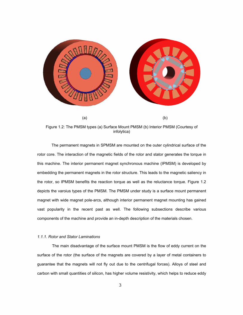
Figure 1.2: The PMSM types (a) Surface Mount PMSM (b) Interior PMSM (Courtesy of infolytica)

The permanent magnets in SPMSM are mounted on the outer cylindrical surface of the

rotor core. The interaction of the magnetic fields of the rotor and stator generates the torque in

this machine. The interior permanent magnet synchronous machine (IPMSM) is developed by

embedding the permanent magnets in the rotor structure. This leads to the magnetic saliency in

the rotor, so IPMSM benefits the reaction torque as well as the reluctance torque. Figure 1.2

depicts the varoius types of the PMSM. The PMSM under study is a surface mount permanent

magnet with wide magnet pole-arcs, although interior permanent magnet mounting has gained

vast popularity in the recent past as well. The following subsections describe various

components of the machine and provide an in-depth description of the materials chosen.

1.1.1. Rotor and Stator Laminations

The main disadvantage of the surface mount PMSM is the flow of eddy current on the

surface of the rotor (the surface of the magnets are covered by a layer of metal containers to

guarantee that the magnets will not fly out due to the centrifugal forces). Alloys of steel and

carbon with small quantities of silicon, has higher volume resistivity, which helps to reduce eddy

4

current losses in the core. Silicon steels are the most popular material used to design

laminations for all families of electric machines where the additional cost is justified by the

increased performance. These steels are available in different grades and thicknesses.

Silicon steels are generally specified and selected on the basis of allowable core loss in

watts/lb. The grades are classified in an increasing order of core loss, by numbers with a prefix

‘M’; i.e. M19, M27, M36, M45 and so on, where each grade specifying a maximum core loss.

Higher M numbers (and thus higher core losses) are significantly cheaper, although only a small

percentage of power is saved with each step down in performance. M19 is probably the most

common grade of steel used for electromechanical energy conversion devices, as it offers

nearly the lowest core loss in this class of material, for a fraction of additional cost.

1.1.2. Permanent Magnet

The Permanent Magnet (PM) is a unique component in the energy conversion process.

Potential energy is stored both in the magnet volume and in the external field associated with

the magnet. They often operate over a dynamic cycle where energy is converted from electrical

or mechanical form to field energy and then returned to the original form. A PM is characterized

and compared in terms of its composition and defined unit properties obtained from the

hysteresis loop of the magnet material.

The earliest manufactured magnet materials were made of hardened steel since

magnets made from steel were easily magnetized. However, they had an inherent disadvantage

of having very low energy and being easy to demagnetize. In recent years other magnet

materials such as Aluminum Nickel and Cobalt alloys (ALNICO), Strontium Ferrite or Barium

Ferrite (Ferrite), Samarium Cobalt (First generation rare earth magnet) (SmCo) and Neodymium

Iron-Boron (Second generation rare earth magnet) (NdFeB) have been developed for this

purpose. The frest of this section gives a brief description of the different magnet materials

commonly used [1].

5

Ceramic of Ferrite magnets are made of a composite of iron oxide and barium

carbonate (BaCO3) or strontium carbonate (SrCO3). This material has been widely available

since the 1950’s and therefore is readily available. A commonly used type of ceramic magnet is

a sintered magnet which is composed of compressed powder of alloy material being used. The

magnets are hard & brittle and generally require diamond wheels to grind & shape. While these

magnets are solid, their physical properties are similar to a ceramic and are therefore easily

broken and chipped. Benefits of ceramic magnets include low cost, high coercive force,

resistance to corrosion, and high heat tolerance. Drawbacks include low energy product (their

strength), low mechanical strength, and the presence of ferrite powder on the surface of the

material which tends to rub off and cause soiling.

Alnico magnet is an alloy of aluminum (Al), nickel (Ni) and cobalt (Co) with little

amounts of other elements added to enhance the properties of the magnet. These magnets

have high corrosion resistance, high mechanical strength and very high working temperatures.

Their drawbacks include higher cost, low coercive force, low energy product and their tendency

to demagnetize due to shocks.

Rare earth magnets are composed of alloys of Lanthanide group of elements.

Neodymium (Nd) and Samarium (Sm) are two most commonly used elements for this family of

magnets. The most popular varieties that are currently in use include neodymium-iron-boron

(Nd2Fe14B, sometimes referred to as NdFeB) and samarium-cobalt (SmCo5, Sm2Co17).

Samarium Cobalt (SmCo) magnets are highly resistant to oxidation, particularly

resistant to temperature (upto 350° C), have higher magnetic strength than ceramic & alnico but

are brittle and prone to chipping & cracking. In addition, due to the high cost of samarium, they

are comparably very expensive. Neodymium-Iron-Boron (NdFeB) magnets are the most

advanced and most popular permanent magnet available today. This material has properties

similar to samarium-cobalt magnets, but is easily oxidized and doesn’t have the same

resistance to temperature. They have a strong residual field, moderate temperature stability, a

6

very high energy product and are more easily shaped. Although NdFeB magnets are more

expensive by mass but their high flux density per unit volume (energy product) contribute to a

compact design, also making it economical to most applications.

Polymer based magnets are composed of the above-mentioned materials with various

polymers to create a broad range of magnetic materials and mechanical properties. This is done

mainly for enhancing material flexibility, shape complexity and direction of magnetic fields. A

distinct drawback of this family of magnets is their low energy product.

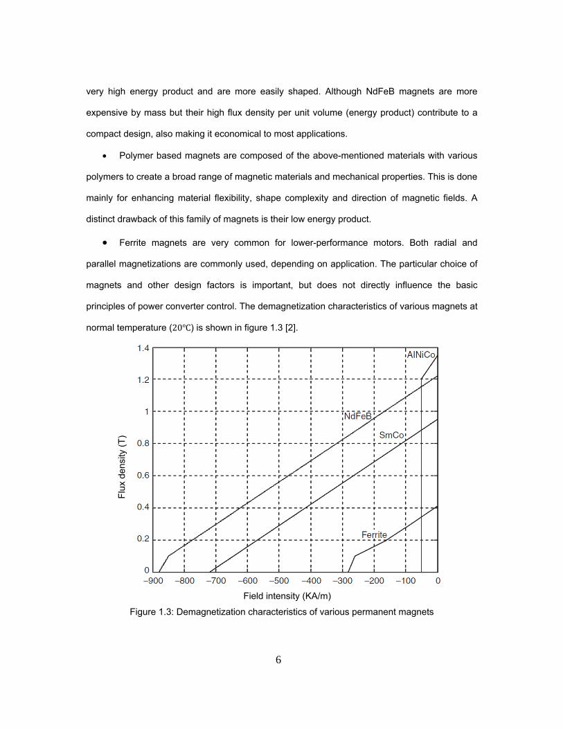
Ferrite magnets are very common for lower-performance motors. Both radial and

parallel magnetizations are commonly used, depending on application. The particular choice of

magnets and other design factors is important, but does not directly influence the basic

principles of power converter control. The demagnetization characteristics of various magnets at

normal temperature (20 ) is shown in figure 1.3 [2].

Flu

x de

nsity

(T

)

Field intensity (KA/m)

Figure 1.3: Demagnetization characteristics of various permanent magnets

7

According to this figure the demagnetization curve of a permanent magnet can be fully

characterized by the following parameters [2]:

Remanent Magnetism ( ) which is where characteristic meets the B-axis.

Coercive field intensity ( ) which is where characteristic meets the H-axis.

Curvature connecting these two points.

In fact, the second linear region that is close to the H-axis is considered as an unstable

region. Therefore a proper operating point will be located in the first linear part, which is

expressed as:

HBB rr 0 (1.1)

Where r and 0 stand for relative and air permeability, respectively. It must be noted

that in permanent magnets r is very close to 1 (relative permeability of the air). Accordingly,

the energy density of a permanent magnet (assuming a linear characteristic) can be computed

as:

)/(4

. 3

0

2

max mKJB

EHBEr

t

(1.2)

It must be mentioned that ferrite magnets represent a low-cost solution while offering a

limited flux density. AlNiCo magnets, which are more expensive as compared to ferrite

magnets, demonstrate a very high remanent magnetism. This, however, is undermined by very

limited corecive field intensity. The most expensive, SmCo magnets, represent quality in every

aspect including high remanent magnetism, large corecive field intensity, and a fully linear

demagnetization characteristic. They also are known as highly stable in the presence of high

temperature variation. Finally, the NdFeB magnets demonstrate very high energy density at

room temperature. Furthermore, the cost associated with NdFeB is much less than SmCo

magnets. However, corecive field intensity in NdFeB magnets is highly sensitive to temperature

changes. This, in turn, results in an inadequate performance at high temperatures. In general,

8

the main objectives in selecting a permanent magnet for motor drive application can be

summarized as [2]:

High energy density.

A linear demagnetization characteristic in the entire vicinity of the second quadrant (B-H

plane).

High stability with respect to temperature.

High specific resistance to mitigate eddy currents.

Durability against corrosion and demagnetization.

Low cost.

Although achieving all these attributes in a single magnet is not possible, proper design

can help us to optimize the performance of the drive in the context of the application. The

magnetic characteristics of various magnets are summarized in table 1.1 [2].

Table 1.1 Permanent magnet characteristics

ferrite AlNiCo SmCo5 NdFeB

Remanent

magnetism ( )(TBr ) 0.38 … 0.42 0.61 … 1.35 0.85 … 1.0 1.0 … 1.23

Corecive field intensity ( /

)

390 … 280 59 … 50 1000 … 1200 1600 … 960

Max. energy density (BHmax [kJ/m3])

28 … 34 13 … 62 140 … 200 195 … 280

Temperature coefficient (KB[%/C])

–0.2 … –0.23 –0.02 –0.04 … –0.05 –0.11 … –0.13

Temperature coefficient (KH[%/C])

0.4 … 0.22 0.03 … –0.07 -0.25 –0.6 … –0.8

Reversible permeability (μrev)

1.05 <5 1.05 <1.2

Density [ρ/(kg/dm3)] 4.6 … 4.9 6.7 … 7.3 8.1 … 8.3 7.3 … 7.4

Specific electric resistance [ρCL/μΩcm]

10 …10

40 … 70 50 … 60 140

Cost [%] 10 … 15 40 … 60 600 … 800 200 … 300

9

Comparing various properties of permanent magnets, the following observation can be

made [2]:

A rise in temperature will reduce the remanent magnetism in all magnet types. On a

percentage basis, ferrite magnets seem to be the most sensitive magnets, while SmCo

demonstrates the least sensitivity.

Corecive field intensity portrays different behavior for various materials. While an

increase in temperature results in significant decrease of corecive field in NdFeB, an

opposite response is seen in ferrite magnets. Overall, SmCo offers the least sensitivity

to temperature.

SmCo is the heaviest and the most expensive alternative among all candidates. It also

presents one of the lowest specific resistances, which translates to high eddy current

losses.

AlNiCo offers the highest remanent magnetism. This, however, is mainly undermined by

a very limited corecive field intensity and extremely high conductivity.

The reversible permeability in most cases is close to 1.

1.2 Fault tolerant operation of PMSM

Fault tolerance has become a design criterion for adjustable speed motor drives

(ASMD) which are used in high impact applications. Fault tolerant motor drives are highly

demanded in many sectors of industry including automotive, aerospace and military and

domestic applications. In simple terms, a fault tolerant ASMD is expected to continue its

intended function in the event of a failure compliment to its remaining components. Knowledge

of magnetic field distribution in electrical machines especially the PMSM has shown to give an

in-depth understanding of machine behavior in terms of force distribution and optimal excitation

determination in various parts of the machine. Based on that, the availability of improved

computational tools to analyze the magnetic field is of great importance. Employment of

10

microscopic electromechanical energy conversion scheme can be employed to give us the

following benefits:

Fault tolerant design.

Optimal excitation for maximum energy conversion ratio (torque/Amp).

Reduction of the torque ripple so the acoustic noise.

Improvement in efficiency.

From an engineering point of view there is a trade off between the following goals, so

depending on the application, some of these items can be of more importance in the design

process. The main purpose of this project is fault tolerance design while the other factors are

sought as much as possible. Fault tolerant operation of an electric drive is a prime objective in

high impact applications. By manipulating the tangential and normal components of magnetic

field in various parts of the machine, the flux can be observed and used to detect the fault

condition. The proposed method offers new numerical techniques for analysis and design of a

PMSM. These techniques are time efficient and offer an insightful version of the magnetic field

in the machine. Target applications for this technique include the following areas:

Automotive

Domestic appliances

Naval and Military

Aerospace systems.

The proposed scheme would combine ideas from electromechanical energy

conversion, signal reconstruction, pattern recognition, and power electronics to create novel

solutions. The successful completion of this target would pave the road for development of cost

effective, highly efficient, fault tolerant, and reliable electric motor drive. The most eminent

attributes of this approach are:

The magnetic filed components have been investigated in various parts of the machine.

The fault detection scheme is based on the flux observation in the machine structure.

11

The optimal excitation of the machine has been derived based on the same knowledge

of the field distribution.

1.3 State-of-the-Art

The ongoing challenges in the design and control of fault tolerant electric drives have

been the focus of many researches [3-8]. However improvements in these areas have been

incremental. Most of the work which is done focuses on the fault tolerant design of the electrical

machine [9-17]. A multi phase drive, in which each phase is regarded as a single module is the

best design for this purpose. These modules should have the minimal impact on each other so

that the failure in one does not affect the others. The modular approach requires:

Minimal electrical interaction: separate single phase bridges can be used for this

purpose [18].

Minimal magnetic interaction: In case of the magnetic coupling between the phases

fault current in one can induce voltages in the other which causes problems especially

in the control process [19].

Minimal thermal interaction: The stator outer surface should be cooled down properly.

Also each stator slot shoul dbe used for one phase winding to separate the thermal

coupling between phases.

Although effective, these techniques are not appropriate in case the design of the

machine is not flexible. Principles of a fault tolerant system have been presented in [20]. For an

electric drive the fault tolerance necessitates the following:

Partitioning and redundancy

Isolation between modules

Fault detection and reporting

Service continuity, Online repair

12

The fault tolerant design has its own disadvantages which can be caused by the

unusual design or the introduction of the redundancy. Fault tolerance has been achieved in [17]

by deploying a dual motor drive configuration. Same method has been used in [21, 22] to obtain

fault tolerance. The disadvantage of this method is that another module of the same size and

price of the main module should be used which increases the cost of the system. Also, the

control strategy would be more complicated in this case. In some applications the weight and

size of the electrical drive is also a restriction so the dual modular system will be inappropriate.

The above mentioned methods generally deal with the fault tolerant design of the machine and

increasing the redundancy of the system under operation. There are cases in which the design

of the machine is not possible and due to the limitations in space and cost, deploying a

secondary back up module is not feasible. In this case the system should be able to detect the

fault and remove it before the remaining healthy parts are damaged. So, there should be

detection schemes that constantly monitor the machine. Also, to guarantee the continous

service there should be schemes to squeeze the maximum power possible out of the machine.

The fault detection schemes can be classified into following:

flux based [23, 24]

current based [25]

In these methods the magnetic flux or the stator currents of the PMSM are monitored

during operation. By performing mathematical analysis, such as FFT, Hilbert transform, etc [23,

24], specific signatures can be detected for each type of fault.

Optimal excitation of the electrical machines has been considered as a useful tool to

improve the overall efficiency of the system [26]. In order to introduce the required redundancy

the sizing of the semiconductors should be judiciously increased. This in turn results in more

silicon and higher expense. Alternatively, the excitation of the machine can be modified in a way

that yields the optimal output of interest. In this study the maximum torque per ampere is of

primary interest. Therefore the target is to find the optimal stator excitation, in the event of a

13

fault, such that the post fault torque per ampere of the machine would be maximized. Our study

uses Maxwell stress tensor method to analyze the torque behavior in normal and post fault

operation. This method provides a detailed and insightful picture of the electromechanical

energy conversion by providing a detailed description of the magnetic field and force

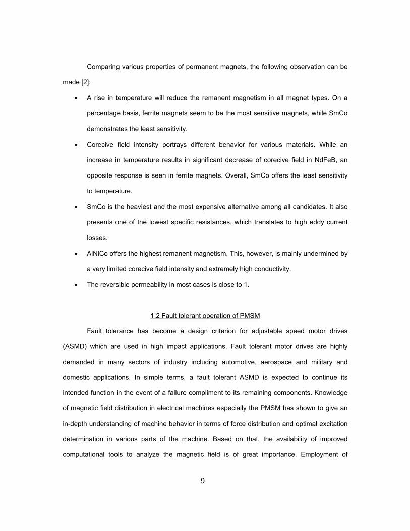
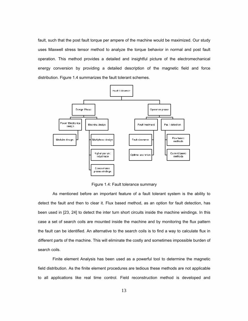
distribution. Figure 1.4 summarizes the fault tolerant schemes.

Figure 1.4: Fault tolerance summary

As mentioned before an important feature of a fault tolerant system is the ability to

detect the fault and then to clear it. Flux based method, as an option for fault detection, has

been used in [23, 24] to detect the inter turn short circuits inside the machine windings. In this

case a set of search coils are mounted inside the machine and by monitoring the flux pattern

the fault can be identified. An alternative to the search coils is to find a way to calculate flux in

different parts of the machine. This will eliminate the costly and sometimes impossible burden of

search coils.

Finite element Analysis has been used as a powerful tool to determine the magnetic

field distribution. As the finite element procedures are tedious these methods are not applicable

to all applications like real time control. Field reconstruction method is developed and

14

implemented to improve the process of finding magnetic field components in the electrical

machines [27-30]. Field reconstruction method provides insight to microscopic

electromechanical energy conversion and can be used as an alternative to FEA to analyze

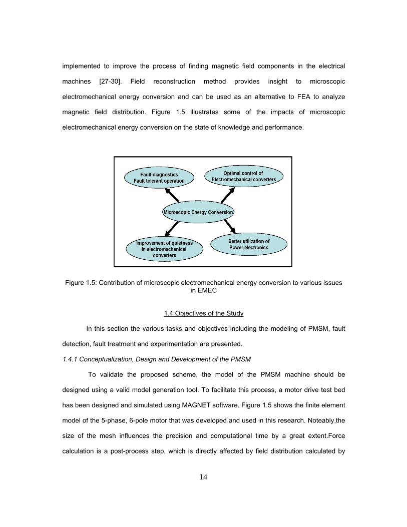
magnetic field distribution. Figure 1.5 illustrates some of the impacts of microscopic

electromechanical energy conversion on the state of knowledge and performance.

Figure 1.5: Contribution of microscopic electromechanical energy conversion to various issues in EMEC

1.4 Objectives of the Study

In this section the various tasks and objectives including the modeling of PMSM, fault

detection, fault treatment and experimentation are presented.

1.4.1 Conceptualization, Design and Development of the PMSM

To validate the proposed scheme, the model of the PMSM machine should be

designed using a valid model generation tool. To facilitate this process, a motor drive test bed

has been designed and simulated using MAGNET software. Figure 1.5 shows the finite element

model of the 5-phase, 6-pole motor that was developed and used in this research. Noteably,the

size of the mesh influences the precision and computational time by a great extent.Force

calculation is a post-process step, which is directly affected by field distribution calculated by

15

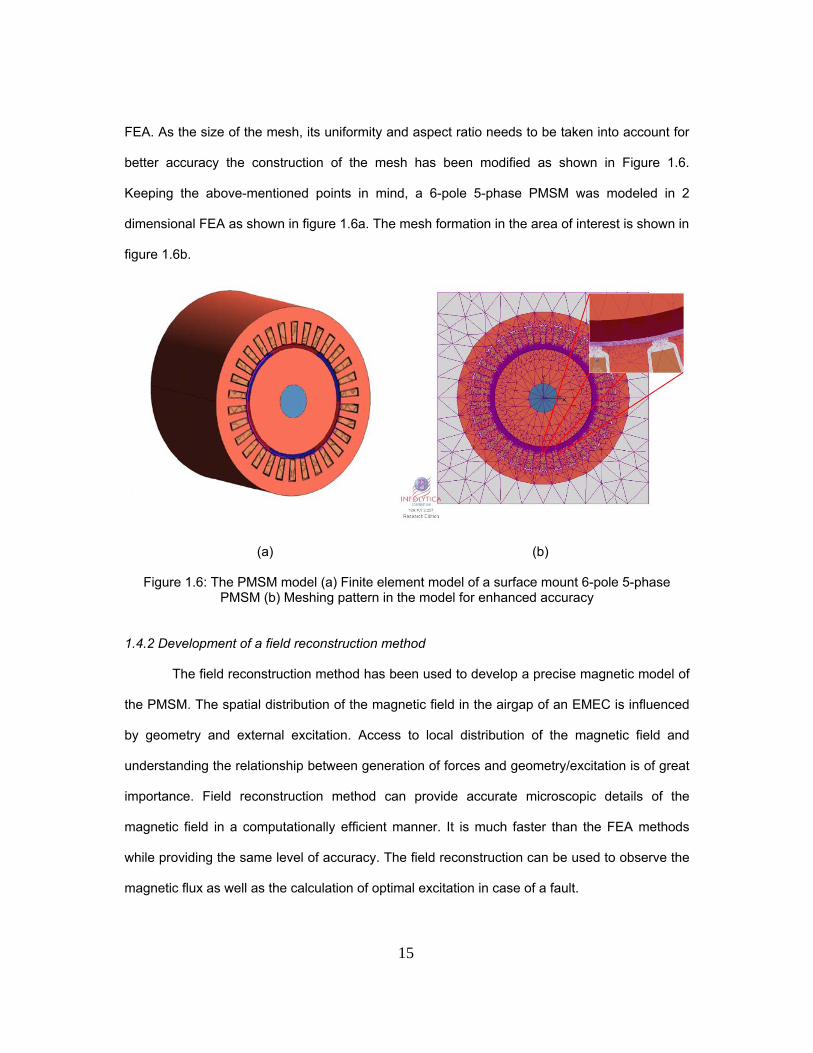
FEA. As the size of the mesh, its uniformity and aspect ratio needs to be taken into account for

better accuracy the construction of the mesh has been modified as shown in Figure 1.6.

Keeping the above-mentioned points in mind, a 6-pole 5-phase PMSM was modeled in 2

dimensional FEA as shown in figure 1.6a. The mesh formation in the area of interest is shown in

figure 1.6b.

(a) (b)

Figure 1.6: The PMSM model (a) Finite element model of a surface mount 6-pole 5-phase PMSM (b) Meshing pattern in the model for enhanced accuracy

1.4.2 Development of a field reconstruction method

The field reconstruction method has been used to develop a precise magnetic model of

the PMSM. The spatial distribution of the magnetic field in the airgap of an EMEC is influenced

by geometry and external excitation. Access to local distribution of the magnetic field and

understanding the relationship between generation of forces and geometry/excitation is of great

importance. Field reconstruction method can provide accurate microscopic details of the

magnetic field in a computationally efficient manner. It is much faster than the FEA methods

while providing the same level of accuracy. The field reconstruction can be used to observe the

magnetic flux as well as the calculation of optimal excitation in case of a fault.

16

1.4.3 Development of fault detection and optimization strategies

The fault tolerant system should be capable of fault detection and remediation. Also, it

is desirable that the PMSM delivers maximum torque per ampere in the event of a fault. A set of

look up tables can be created for each kind of fault and by monitoring the flux the type of fault

can be detected. Also, based on the type of fault that happens and the place of occurrence the

optimal excitation should be deployed to improve the machine performance.

1.4.4 Development of an experimental test bed

The conventional PMSM can become fault tolerant using the proposed method. For the

validation of the proposed scheme, an experimental PMSM drive was designed and constructed

at the Renewable Energy and Vehicular Technology Lab. This experimental system is used for

validation of the flux estimation as well as the optimized fault tolerant performance using field

reconstruction method. Fault detection and removal and optimization of the remaining healthy

machine phase excitations are the main objectives in this experimental investigation.

1.5 Outline of the dissertation

The state-of-the-art investigation, problem identification, modeling, detection and

treatment of fault tolerant PMSM are presented here. This dissertation includes 5 chapters

whose outline is as follows:

Chapter 2 describes the fundamentals of the field reconstruction method. In this

chapter the FRM is developed and implemented for the PMSM. To validate this model a finite

element model is also created for comparison purposes. Maxwell Stress Tensor method is used

to quantify electromagnetic torque in the middle of the airgap.

Chapter 3 deals with the mehtods of flux estimation in permanent magnet synchronous

machines. The traditional flux estimation technique is discussed and the novel methods will be

introduced in detail. These novel methods are supported by experimental and simulation

results.

17

Chapter 4 introduces various faults under study, detection schemes and optimization

strategies. The stator inter turn short circuit fault on single or multiple phases, rotor partial

demagnetization and rotor eccentricity are investigated in this chapter. The experimental setup

is used to support the theory and simulations.

Chapter 5 summarizes the achievements of this study and provides concluding

comments on the findings.

18

CHAPTER 2

FIELD RECONSTRUCTION METHOD

Electromechanical energy conversion in energy conversion devices occurs in terms of

magnetic fields from the media within which the electromechanical energy conversion takes

place. Magnetic fields provide a controllable means within a relatively compact and highly

efficient environment for energy conversion. Once the electromechanical energy converter is

supplied with electric current, a magnetic field throuout the device is established. Using Maxwell

stress tensor method, distribution of the radial and tangential force densities in the airgap of the

machine can be expressed as:

)(2

1 22

0tnn BBf

(2.1)

)(1

0tnt BBf

(2.2)

Where 0and,,,, tntn BBff denote normal and tangential component of the force

density in the airgap, normal component of flux density, tangential component of flux density,

and air magnetic permeability respectively. Tangential forces are partially responsible for the

generation of torque on the rotor and tangential vibration of the stator frame. The tangential

forces that are produced on the stator poles cause unwanted vibration in the stator frame. The

resultant forces acting on the machine components can be determined by integrating the

tangential and radial force densities on the surface of the desired component as follows:

S

tt dsfF .

(2.3)

snn drflF

2

0

(2.4)

19

Where s denotes the outer surface of a cylinder located in the airgap of the machine

and l, r,ands denote stack length, radius of the integrating contour, and angle component in

cylindrical system of coordinates respectively.

Bn(

T)

Rotor Position(Deg)

(a)

Bt(

T)

Rotor Position(Deg)

(b) Figure 2.1: magnetic flux density in the middle of the airgap (a) Normal component (b)

Tangential component

0 30 60 90 120 150 180 210 240 270 300 330 360-0.8

-0.6

-0.4

-0.2

0

0.2

0.4

0.6

0.8

0 30 60 90 120 150 180 210 240 270 300 330 360-0.4

-0.3

-0.2

-0.1

0

0.1

0.2

0.3

0.4

20

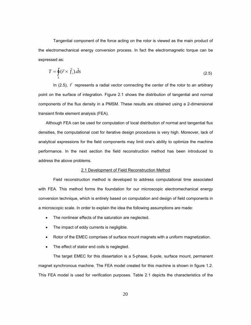
Tangential component of the force acting on the rotor is viewed as the main product of

the electromechanical energy conversion process. In fact the electromagnetic torque can be

expressed as:

sdfrTS

t

).( (2.5)

In (2.5), r

represents a radial vector connecting the center of the rotor to an arbitrary

point on the surface of integration. Figure 2.1 shows the distribution of tangential and normal

components of the flux density in a PMSM. These results are obtained using a 2-dimensional

transient finite element analysis (FEA).

Although FEA can be used for computation of local distribution of normal and tangential flux

densities, the computational cost for iterative design procedures is very high. Moreover, lack of

analytical expressions for the field components may limit one’s ability to optimize the machine

performance. In the next section the field reconstruction method has been introduced to

address the above problems.

2.1 Development of Field Reconstruction Method

Field reconstruction method is developed to address computational time associated

with FEA. This method forms the foundation for our microscopic electromechanical energy

conversion technique, which is entirely based on computation and design of field components in

a microscopic scale. In order to explain the idea the following assumptions are made:

The nonlinear effects of the saturation are neglected.

The impact of eddy currents is negligible.

Rotor of the EMEC comprises of surface mount magnets with a uniform magnetization.

The effect of stator end coils is neglegted.

The target EMEC for this dissertation is a 5-phase, 6-pole, surface mount, permanent

magnet synchronous machine. The FEA model created for this machine is shown in figure 1.2.

This FEA model is used for verification purposes. Table 2.1 depicts the characteristics of the

21

permanent magnet machine. Figure 2.2 shows the cross section of this machine that has been

cut and rolled along the neutral axis of a pair of rotor poles.

Table 2.1 Target PMSM characteristics

Rated Power 10 hp Number of Phases 5

Rated Speed 1800 rpm Number of Poles 6 Number of Stator

Slots 30

Stator Winding Material

Copper

Stator back iron Material

M19

Type of Permanent magnets

Surface Mount

Rotor Material M19 Shaft Material Cold rolled Steel Stack length 6 in.

N Sg

1 . . . mi i

s 02

P

N Sg

1 . . . mi i

s 02

P

Figure 2.2: Cross section of the slot-less PM machine

In Figure 2.2, s represents the displacement for any point on the stator and mii .....1

represent the current in each conductor. In this configuration, the normal and tangential

components of the flux density due to surface mounted permanent magnets are defined as

,n pmB and pmtB , respectively. Each conductor on the stator contributes to the tangential and

radial components of the flux density in the airgap. The tangential and normal components of

the flux density that are contributed by a conductor (representing the thk phase) located at sk

are given as follows:

22

,

,

2( ) ( ) 0

( ) ( )

t k t k t s sk s

n k n k n s sk

B B i hP

B B i h

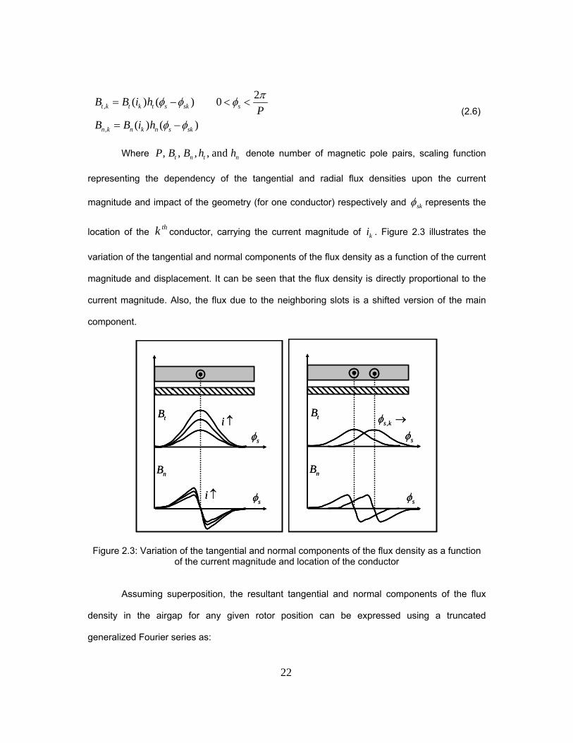
(2.6)

Where , , , , andt n t nP B B h h denote number of magnetic pole pairs, scaling function

representing the dependency of the tangential and radial flux densities upon the current

magnitude and impact of the geometry (for one conductor) respectively and sk represents the

location of the thk conductor, carrying the current magnitude of ki . Figure 2.3 illustrates the

variation of the tangential and normal components of the flux density as a function of the current

magnitude and displacement. It can be seen that the flux density is directly proportional to the

current magnitude. Also, the flux due to the neighboring slots is a shifted version of the main

component.

tB

nB

s

si

i

tB

nB

s

si

i

tB

nB

s

s,s k tB

nB

s

s,s k

Figure 2.3: Variation of the tangential and normal components of the flux density as a function of the current magnitude and location of the conductor

Assuming superposition, the resultant tangential and normal components of the flux

density in the airgap for any given rotor position can be expressed using a truncated

generalized Fourier series as:

23

)()(),...,,(

)()(),...,,(

1,,1

1,,1

sksnk

m

kknpmnmsn

skstk

m

kktpmtmst

hiBBiiB

hiBBiiB

(2.7)

The above expressions depict an elegant illustration of the separation between factors

influenced by geometry (i.e. ,th and nh ) and external excitation (i.e. ,,ktB and knB , ).

Accordingly, the tangential and normal components of the force densities can be computed as

follows:

1 1 10

2 21 1 1

0

1( , ,... ) ( , ,... ) ( , ,... )

1( , ,... ) ( , ,... ) ( , ,... )

2

t s m t s m n s m

n s m n s m t s m

f i i B i i B i i

f i i B i i B i i

(2.8)

In order to calculate the resultant forces for each rotor position, one needs to integrate

the force densities over the outer surface of a cylinder which is located in the middle of the

airgap:

2

1

0

2

1

0

2( ) . . ( , ,... ) 0

( ) . . ( , ,... )

P

t r t s m s r

P

n r n s m s

F P L R f i i dP

F P L R f i i d

(2.9)

Where , , andr L R represent rotor position, stack length of the machine, and radius of

the integration surface respectively. In this computation a two dimensional symmetry in the

geometry of the machine is assumed. As can be observed detection of the basis functions ,th

and nh play a central role in the formulation of the field reconstruction. Under unsaturated

conditions the scaling functions representing the external excitation are linear functions of the

relevant currents, i.e.:

24

knkkn

kkkkt

iBiB

iBiB

.)(

.)(

,

,

(2.10)

Once the pattern of excitation is known and basis functions are identified, one can use

(2.7) through (2.9) to identify the distribution of field/force for a given position. It must be noted

that the contribution of the permanent magnets are assumed as a separate input to (2.7).

Analysis of an unsaturated slot-less stator with an embedded conductor (figure 2.2) indicates

that the basis functions, th and nh have the following properties:

(a) Periodic with respect to s ,

(b) th has an even symmetry with respect to s ,

(c) nh has an odd symmetry with respect to s .

Therefore, without rotor excitation (winding or permanent magnet) the resultant

tangential force will be an odd function resulting in zero average torque at every given point.

However, the radial forces will exist even without any magnetic source on the rotor. One of the

most important tasks of this dissertation will be to identify analytical expressions of the basis

functions ,th and nh for the 5 phase permanent magnet synchronous machine.

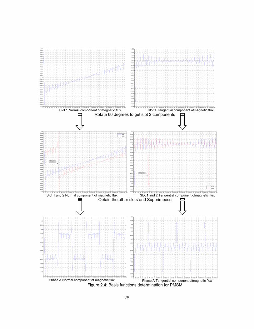
Figure 2.4 shows the process of reconstruction of the flux density due to the permanent

magnets and the stator phase winding currents. In this process, as the figure describes, 1A

current is first applied to the conductors in a single slot of the machine. The flux density

obtained due to this unit current is called the “basis function” for the given geometry. This

function should be rotated by 60 degrees and superimposed to achieve the field distribution due

to the current in one phase. Further, as the in the balanced 5 phase systems the consecutive

phases are 72 degrees apart,this plot is rotated by 72 electrical degrees and superimposed to

estimate the effective field due to current in all five phases of the machine. It must be mentioned

that the flux from the permanent magnet is unchanged in magnitude. It simply rotates with rotor

position.

25

Slot 1 Normal component of magnetic flux Slot 1 Tangential component ofmagnetic fluxRotate 60 degrees to get slot 2 components

Slot 1 and 2 Normal component of magnetic flux Slot 1 and 2 Tangential component ofmagnetic fluxObtain the other slots and Superimpose

Phase A Normal component of magnetic flux Phase A Tangential component ofmagnetic fluxFigure 2.4: Basis functions determination for PMSM

0 10 20 30 40 50 60 70 80 90 100 110 120 130 140 150 160 170 180 190 200 210 220 230 240 250 260 270 280 290 300 310 320 330 340 350 360-0.03

-0.028

-0.026

-0.024

-0.022

-0.02

-0.018

-0.016

-0.014

-0.012

-0.01

-0.008

-0.006

-0.004

-0.002

0

0.002

0.004

0.006

0.008

0.01

0.012

0.014

0.016

0.018

0.02

0.022

0.024

0.026

0.028

0.03

Slot1

Slot2

60 degrees

0 10 20 30 40 50 60 70 80 90 100 110 120 130 140 150 160 170 180 190 200 210 220 230 240 250 260 270 280 290 300 310 320 330 340 350 360-0.036

-0.034

-0.032

-0.03

-0.028

-0.026

-0.024

-0.022

-0.02

-0.018

-0.016

-0.014

-0.012

-0.01

-0.008

-0.006

-0.004

-0.002

0

0.002

0.004

0.006

0.008

0.01

Slot 1

Slot 2

60 degrees

0 10 20 30 40 50 60 70 80 90 100 110 120 130 140 150 160 170 180 190 200 210 220 230 240 250 260 270 280 290 300 310 320 330 340 350 360

-0.03

-0.025

-0.02

-0.015

-0.01

-0.005

0

0.005

0.01

0.015

0.02

0.025

0.03

0 10 20 30 40 50 60 70 80 90 100 110 120 130 140 150 160 170 180 190 200 210 220 230 240 250 260 270 280 290 300 310 320 330 340 350 360-0.04

-0.035

-0.03

-0.025

-0.02

-0.015

-0.01

-0.005

0

0.005

0.01

0.015

0.02

0.025

0.03

0.035

0.04

0 10 20 30 40 50 60 70 80 90 100 110 120 130 140 150 160 170 180 190 200 210 220 230 240 250 260 270 280 290 300 310 320 330 340 350 360-0.035

-0.033

-0.031

-0.029

-0.027

-0.025

-0.023

-0.021

-0.019

-0.017

-0.015

-0.013

-0.011

-0.009

-0.007

-0.005

-0.003

-0.001

0.001

0.003

0.005

0.007

0.0090.01

0 10 20 30 40 50 60 70 80 90 100 110 120 130 140 150 160 170 180 190 200 210 220 230 240 250 260 270 280 290 300 310 320 330 340 350 360-0.03

-0.028

-0.026

-0.024

-0.022

-0.02

-0.018

-0.016

-0.014

-0.012

-0.01

-0.008

-0.006

-0.004

-0.002

0

0.002

0.004

0.006

0.008

0.01

0.012

0.014

0.016

0.018

0.02

0.022

0.024

0.026

0.028

0.03

26

Phase A Normal component of magnetic flux Phase A Tangential component ofmagnetic flux

PM contribution to Normal component of magnetic flux PM contribution to Tangential component of magnetic flux

Normal component of magnetic flux Tangential component of magnetic flux Figure 2.5: Magnetic flux determination for PMSM

0 10 20 30 40 50 60 70 80 90 100 110 120 130 140 150 160 170 180 190 200 210 220 230 240 250 260 270 280 290 300 310 320 330 340 350 360

-0.03

-0.025

-0.02

-0.015

-0.01

-0.005

0

0.005

0.01

0.015

0.02

0.025

0.03

0 10 20 30 40 50 60 70 80 90 100 110 120 130 140 150 160 170 180 190 200 210 220 230 240 250 260 270 280 290 300 310 320 330 340 350 360-0.04

-0.035

-0.03

-0.025

-0.02

-0.015

-0.01

-0.005

0

0.005

0.01

0.015

0.02

0.025

0.03

0.035

0.04

0 12 24 36 48 60 72 84 96 108 120 132 144 156 168 180 192 204 216 228 240 252 264 276 288 300 312 324 336 348 360-0.4

-0.35

-0.3

-0.25

-0.2

-0.15

-0.1

-0.05

0

0.05

0.1

0.15

0.2

0.25

0.3

0.35

0.4co t but o

0 12 24 36 48 60 72 84 96 108 120 132 144 156 168 180 192 204 216 228 240 252 264 276 288 300 312 324 336 348 360-0.2

-0.175

-0.15

-0.125

-0.1

-0.075

-0.05

-0.025

0

0.025

0.05

0.075

0.1

0.125

0.15

0.175

0.2

0 30 60 90 120 150 180 210 240 270 300 330 360-0.8

-0.6

-0.4

-0.2

0

0.2

0.4

0.6

0.8

()

0 30 60 90 120 150 180 210 240 270 300 330 360-0.4

-0.3

-0.2

-0.1

0

0.1

0.2

0.3

0.4

()

27

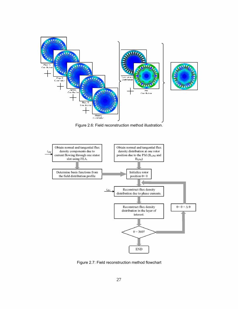
Figure 2.6: Field reconstruction method illustration.

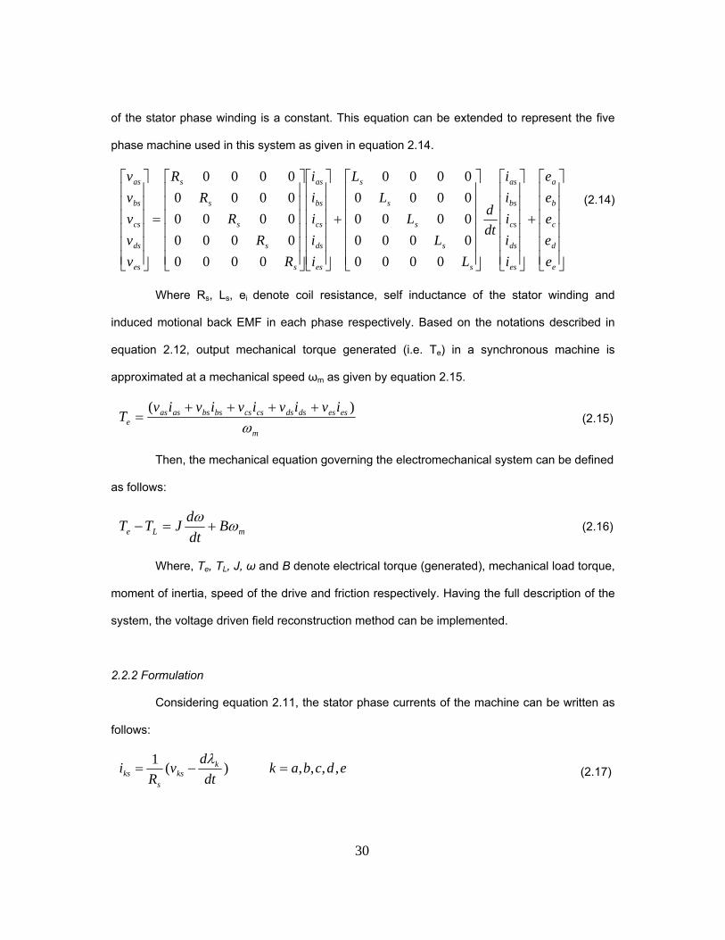
Figure 2.7: Field reconstruction method flowchart

28

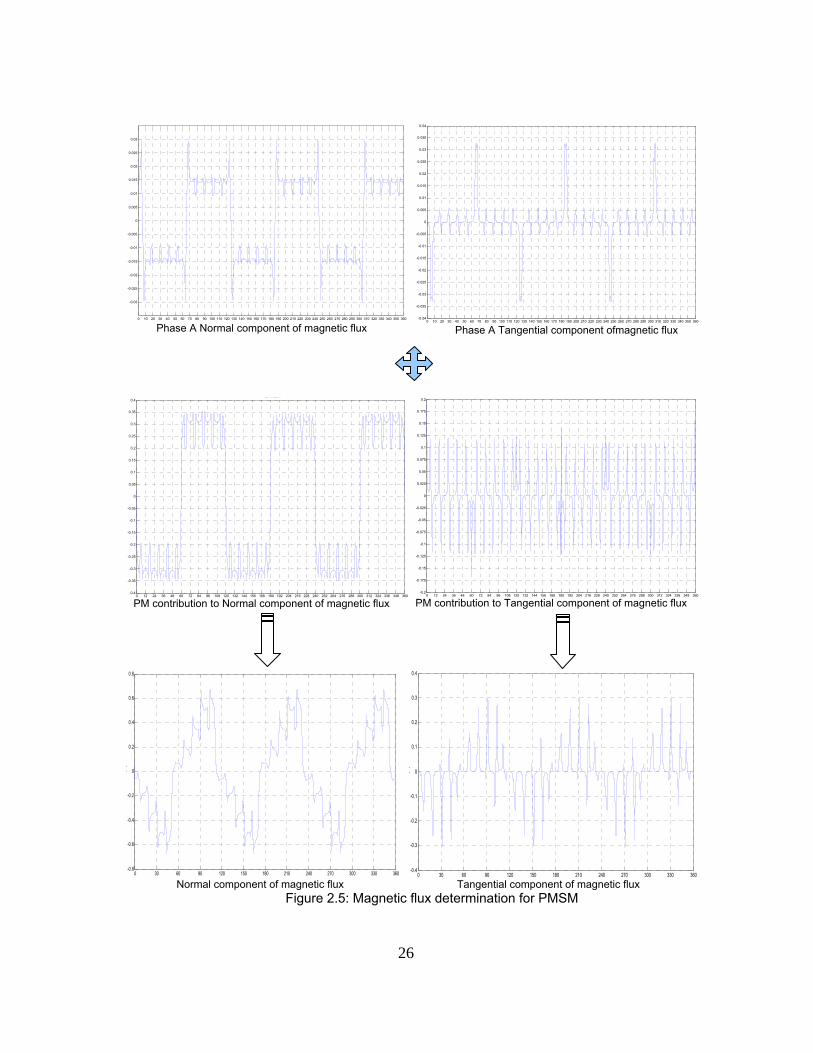
Therefore addition of the fields due to the PM and five phase currents can be used to

estimate flux distribution due to any waveform of current applied to the machine. This process is

done offline and the basis functions are stored as well as the PM contribution. The basis

functions calculation in this way is much faster than the case of the complete system because

there is only one source of magneto-motive force (MMF) in the machine during the calculation

of basis functions. This proves to be one of the major advantages of field reconstruction

method. Also, this method can be applied to any type of stator current and is not just sinusoidal

excitation. Figure 2.4 depicts the basis function determination for the 5 phase PM machine

under study. These functions are added to the PM contribution to achive the complete system

magnetic flux. The field reconstruction method is illustrated in Figures 2.5 and 2.6. According to

these figure the stator phase current contribution is calculated first. Then the PM contribution is

calculated and added to the stator flux to achieve the magnetic flux distribution of the complete

system. The field reconstruction flowchart has been shown in Figure 2.7. In this flowchart the

above modeling procedure is explained.

2.2 Voltage Driven FRM for PMSM

The field reconstruction method descibed in section 2.1 attains the distribution of the

magnetic field based on the instantaneous value of the phase currents. In some applications,

the permanent magnet machine is fed by a voltage source instead of the current source. In that

case the field reconstruction method should be modified to account for the voltage driven

applications. In order to formulize the voltage driven field reconstruction the characteristic

terminal equations of the machine should be investigated.

2.2.1 Electromechanical Description

There are three basic components to be considered in order to fully describe an

electromechanical device, the voltage equation, the flux linkage equation and the torque

equation. The equivalent circuit of the machine, at standstill, phase winding can be modeled as

29

a series combination of the coil resistance and inductance of the winding. Figure 2.8 depicts this

equivalent circuit.

Figure 2.8: Equivalent circuit model for phase winding of the PMSM.

According to Faraday’s law, the voltage equation of the series circuit is defined as the

algebraic sum of the ohmic drop on the resistive element and the rate of change in flux linkage

on the inductive component as follows:

edcbakdt

dRiv k

ksks ,,,,

(2.11)

In this equation, isv and isi are voltages and currents of the 5 phase stator windings

respectively. r and i are the stator winding resistance and phase flux linkages. Equation (2.11)

can be rewritten and expanded as:

es

ds

cs

bs

as

s

s

s

s

s

es

ds

cs

bs

as

s

s

s

s

s

es

ds

cs

bs

as

i

i

i

i

i

dt

d

L

L

L

L

L

i

i

i

i

i

R

R

R

R

R

v

v

v

v

v

0000

0000

0000

0000

0000

0000

0000

0000

0000

0000

(2.12)

Including the effect of back motional EMF, equation 2.11 can be modified to express

the equation in terms of Ohm’s law as in equation 2.13:

bs Edt

diLRiV (2.13)

Where Vs, R, L, λs and i denote phase voltage, winding resistance, phase inductance,

flux linkage across each phase and phase current respectively. In this equation, the resistance

30

of the stator phase winding is a constant. This equation can be extended to represent the five

phase machine used in this system as given in equation 2.14.

e

d

c

b

a

es

ds

cs

bs

as

s

s

s

s

s

es

ds

cs

bs

as

s

s

s

s

s

es

ds

cs

bs

as

e

e

e

e

e

i

i

i

i

i

dt

d

L

L

L

L

L

i

i

i

i

i

R

R

R

R

R

v

v

v

v

v

0000

0000

0000

0000

0000

0000

0000

0000

0000

0000

(2.14)

Where Rs, Ls, ei denote coil resistance, self inductance of the stator winding and

induced motional back EMF in each phase respectively. Based on the notations described in

equation 2.12, output mechanical torque generated (i.e. Te) in a synchronous machine is

approximated at a mechanical speed ωm as given by equation 2.15.

m

esesdsdscscsbsbsasase

ivivivivivT

)(

(2.15)

Then, the mechanical equation governing the electromechanical system can be defined

as follows:

mLe Bdt

dJTT

(2.16)

Where, Te, TL, J, ω and B denote electrical torque (generated), mechanical load torque,

moment of inertia, speed of the drive and friction respectively. Having the full description of the

system, the voltage driven field reconstruction method can be implemented.

2.2.2 Formulation

Considering equation 2.11, the stator phase currents of the machine can be written as

follows:

edcbakdt

dv

Ri k

kss

ks ,,,,)(1

(2.17)

31

For the PMSM under study the input stator phase volatges ( ksv ) are known. Also, the

stator resistances can be measured directly. Having the flux linkages for each stator phase

equation 2.17 can be calculated to attain the stator phase currents. These currents can then be

fed into the field reconstruction module to achieve the magnetic field distribution. The voltage

equations in dq-axes coordinates for a permanent magnet machine can be written as [31]:

ssss

dsqsdssds

qsdsqssqs

pirv

pirv

pirv

000

(2.18)

Where sr and are the coil resistance and reference frame speed, respectively. The

flux linkages can be written as follows:

slss

mslsssmdsssds

qsssqs

iL

LLLiL

iL

00

'

2

3

(2.19)

msL and lsL are magnetizing and leakage inductances, respectively. Using the above

equations:

'

1

1

1

1 0

)(

)(

)(

)(

mkds

kqsss

kds

kqs

ti

tiL

t

t

(2.20)

So:

'

1

1

1

1 0

)(

)(1

)(

)(

mkds

kqs

sskds

kqs

t

t

Lti

ti

(2.21)

Equation 2.18 can be rewritten as:

32

qsdssdsds

dsqssqsqs

irvdt

d

irvdt

d

(2.22)

So:

))()()(()()(

))()()(()()(

111

111

kqskdsskdskdskds

kdskqsskqskqskqs

ttirtvdttt

ttirtvdttt

(2.23)

Equation 2.23 can be rewritten as:

))()()(()()(

))()()(()()(

'111

111

kqsmss

skds

ss

skdskdskds

kdskqsss

skqskqskqs

tL

rt

L

rtvdttt

ttL

rtvdttt

(2.24)

So:

))()(()()1)((

))()(()()1)((

'11

11

kqsmss

skdskds

ss

skds

kdskqskqsss

skqs

tL

rtvdtt

L

dtrt

ttvdttL

dtrt

(2.25)

Finally:

))(()()1(

1))()(()()(

))()(()()1(

1)(

))()(()()1(

1)(

1001010010

'11

11

ksks

ls

sks

ls

sksksks

kqsmss

skdskds

ss

skds

kdskqskqs

ss

skqs

tvdtt

L

dtrt

L

rtvdttt

tL

rtvdtt

L

dtrt

ttvdtt

L

dtrt

(2.26)

Using equation 2.26, the flux linkages of each phase can be determined in terms of

stator applied voltage. The flux linkages then will be used to derive current values using

equation 2.17.

33

2.3 Comparison of Finite Element and Field Reconstruction

In order to validate the PMSM model the finite element analysis has been compared

with the field reconstruction method in this section. This comparison includes the accuracy of

the method and the time required to perform the analysis.

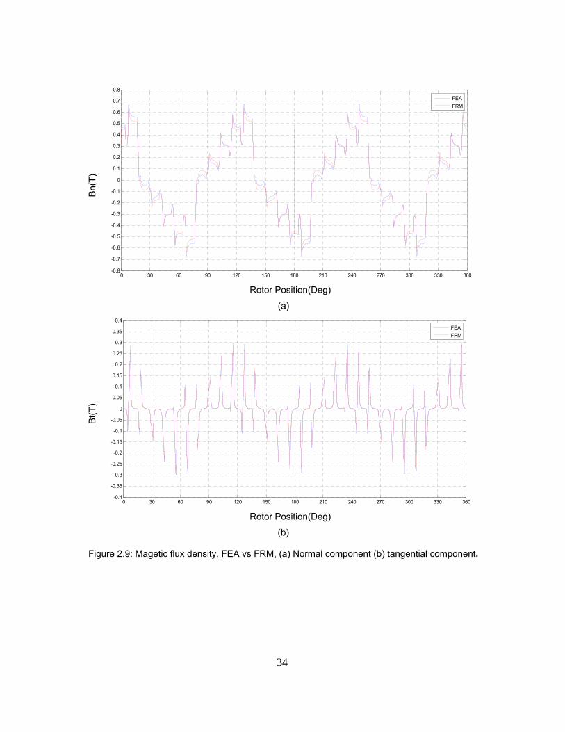
2.3.1 Accuracy

As stated before, field reconstruction method is developed as a replacement tool for

magnetic field analysis. Finite element analysis (FEA) which is the most popular method of

magnetic field analysis is chosen as a reference for comparison purposes. Figure 2.9 depicts

the normal and tangential components of magnetic flux density calculated using field

reconstruction method compared with those obtained using the finite element analysis. In this

case the balanced sinusoidal currents have been applied to stator phase windings and motor is

rotating at a constant speed. According to these figures the magnetic flux densities calculated

using field reconstruction method fits properly to those of the finite element analysis. This

accuracy can be even better in case the mesh used to calculate the basis functions would be of

higher density. As the basis function derivation is a single magneto-static analysis, using a more

dense mesh would not significantly increase the computational time necessary for field

reconstruction. Having these magnetic flux densities and using Maxwell Stress Tensor (MST)

method the electrical torque generated can be calculated. The torque calculated from FRM is

compared wth that of the FEA as shown in Figure 2.10. The back emf of the machine measured

from the experimental set up is compared to that of the field reconstruction as shown in Figure

2.11.

34

Bn(

T)

Rotor Position(Deg)

(a)

Bt(

T)

Rotor Position(Deg)

(b)

Figure 2.9: Magetic flux density, FEA vs FRM, (a) Normal component (b) tangential component.

0 30 60 90 120 150 180 210 240 270 300 330 360-0.8

-0.7

-0.6

-0.5

-0.4

-0.3

-0.2

-0.1

0

0.1

0.2

0.3

0.4

0.5

0.6

0.7

0.8

FEA

FRM

0 30 60 90 120 150 180 210 240 270 300 330 360-0.4

-0.35

-0.3

-0.25

-0.2

-0.15

-0.1

-0.05

0

0.05

0.1

0.15

0.2

0.25

0.3

0.35

0.4

FEA

FRM

35

Tor

que

(Nm

)

Rotor Position(Deg)

Figure 2.10: FEA and FRM torque comparison

2.3.2 Computational time

The main contribution of the field reconstruction method is the computational time which

is much shorter than the conventional finite element procedures. This property makes FRM

suitable for real time control applications. Besides, the shorter computational time translates

into less computational costs from an economical point of view. The method has been tested on

a Pentium 5, 3 GHz processor for simulation purposes. The analysis using FRM takes 30

seconds while the same analysis using FEA takes 8 hours. So, FRM provides accurate enough

results while the computation time is much shorter than the FEA.

Another method ofcomputational time investigation is to implement the process on a

DSP. The target device for this purpose is TMS 320F2812 dsp board. The finite element

analysis can not be implemented on this DSP because of the limitations on the storage and

ALU units.

0 5 10 15 20 25 30 35 40 45 50 55 60 65 70 75 80 85 90 95 100 105 110 115 1200

2

4

6

8

10

12

14

16

18

20

22

24

26

28

30

32

34

36

38

40

42

FEA

FRM

36

(a)

Bac

k E

MF

(V

)

Rotor Position(Deg)

(b)

Figure 2.11: Back EMF comparison, (a) Experimental (b) field reconstruction.

0 30 60 90 120 150 180 210 240 270 300 330 360-28

-26

-24

-22

-20

-18

-16

-14

-12

-10

-8

-6

-4

-2

0

2

4

6

8

10

12

14

16

18

20

22

24

26

28

37

In order to calculate the FRM, the following tasks should be done:

Basis functions should be fetched from memory (10 cycles)

Multiplication of basis functions to the current magnitude (4 cycles)

Addition of the modulated basis functions to achieve stator contribution to magnetic flux

(4 cycles)

Addition of PM contribution to the Stator contribution to achieve complete system

response(4 cycles)

As the clock frequency of this DSP is 150 MHz. each cycle takes almost 6.6 ns. It

means that calculation of each time sample (which is 70 cycles) can be carried out in 462 ns.

The A/D frequency for this DSP is 12 MHz so each conversion takes 83 ns. As the 5 phase

currents and position should be read and converted the overall conversion time will be 498 ns.

The overall calculation time is 960 ns. This short calculation time proves that FRM can be used

in real time control applications where the fast response time is of great importance. The control

loop implemenetd in DSP takes 3 us. So the overall time for calculation and control is almost 4

us. So, the maximum switching frequency possible is 250 MHz which is much bigger than the

average switching frequency of 20 KHz.

38

CHAPTER 3

FLUX ESTIMATION USING FRM

Magnetic flux estimation is one of the main requirements in control of electrical

machines such as direct torque control (DTC) and sensorless operation. There are also fault

detection schemes that work based on the magnetic flux observation. The DTC method, for

example, is used increasingly in motor control applications because of advantages such as fast

dynamic response and minimal dependency on knowledge of the machine parameters. An

issue in using the DTC method is obtaining an accurate estimation of the magnetic flux. Position

sensorless methods are aslo being used to lower cost, reduce size, eliminate sensor cables and

circuitry, and achieve better reliability.

Significant research has been reported on development of sensorless control strategies

[32]–[37]. In this family of control methods, the stator flux linkage is usually calculated by

integrating the voltage across the stator windings using:

,....,,)(0

CBAidtrivt

sisisi (3.1)

Where, siv , r and sii are stator phase voltage, stator resistance, and stator current

respectively. Although straightforward, this method has its own weaknesses which include:

Integration drifts due to offset error in current and voltage measurement.

Errors due to variation in stator resistance as a result of temperature changes, etc.

These challenges become more severe at low speeds when the voltage drop across a

stator resistor is comparable to that of the back-EMF of the machine.

A great deal of research has been done to address these issues. Chapuis and Roye

proposed a constant DC offset method to eliminate the integration drift [38]. This method is

39

useful provided that the offset remains unchanged during the control process. Patel, et_al,

presented a cascaded low pass filter (LPF) method [39] to remedy the problem. Rahman, et_al,

developed low pass filtering (LPF) method for DTC in interior permanent magnet motor drives

[40]. In this method, rather than a standard integrator, an LPF is used. It has been shown that in

the case of a pure DC input signal, the integration method will not diverge, if the exact values of

the system parameters are known [41]. Some research has been carried out to address the

inevitable inaccuracies related to stator resistance. Fuzzy logic techniques have been used in

[42] – [44] to tune the resistance values in DTC.

As mentioned before, besides the DTC, flux observers can be used in conjunction with

specific fault detection schemes for fault tolerance motor drive and control application [45], [46].

Levi, et_al, proposed a stator resistance estimation scheme for the rotor flux-based model

reference adaptive system [47].

Habetler, et_al, presented a model-based stator resistance estimation scheme for

winding temperature monitoring applications [48]. The proposed method is accurate for steady

state operation, while not addressing the low speed problem. All of these methods are

dependant upon machine parameters such as resistance or inductance. Also, the voltage,

current and speed must be monitored precisely.

A Lumped parameter method is another way to estimate the flux linkages of each stator

phase. Assuming the sinusoidal distribution of the stator windings the q- axis and d-axis

components of the flux linkage can be determined as follows:

pmdsdds iL ' (3.2)

qsqqs iL (3.3)

Where, dL and qL are d and q axes inductances respectively. pm' , is the magnetic

flux due to the permanent magnets. Although precise, the main drawback of this method is that

the motional back-emf must be sinusoidal. In case of a small motor with low number of slots per

40

pole per phase, sinusoidal distribution of the windings is not achiveable. As a result lumped

parameter model may not be suitable. This chapter presents a new method of magnetic flux

estimation to remedy the aforementioned issues. The distribution of the magnetic field in the

airgap of the machine is used to estimate flux linkages. Due to the fact that this method is

independent from stator resistance value, the corresponding errors are eliminated. Furthermore,

there is no integration with respect to time, which is prone to numerical drift. This eliminates the

accumulation of errors at low speeds where integration would otherwise take place over a

relatively longer period of time. As a result, magnetic flux can be computed accurately over the

entire speed range.

3.1 Stator Tooth Flux Estimation

In this section the observations and findings which leads to the development of new flux

estimation method has been discussed.

3.1.1 Method 1

The first step in each analysis is the observation of the phenomenon and its behavior in

the operation range. Here, the finite element model created for the 5-phase PMSM is used to

observe the behavior of the magnetic field in the machine. Figure 3.1 depicts the distribution of

the magnetic field in the machine.

Figure 3.1: Magnetic Flux distribution in the machine

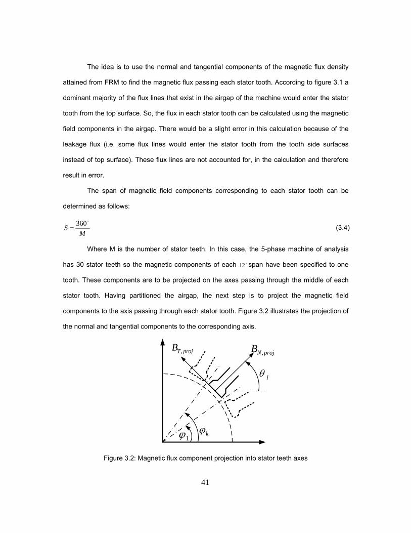
41

The idea is to use the normal and tangential components of the magnetic flux density

attained from FRM to find the magnetic flux passing each stator tooth. According to figure 3.1 a

dominant majority of the flux lines that exist in the airgap of the machine would enter the stator

tooth from the top surface. So, the flux in each stator tooth can be calculated using the magnetic

field components in the airgap. There would be a slight error in this calculation because of the

leakage flux (i.e. some flux lines would enter the stator tooth from the tooth side surfaces

instead of top surface). These flux lines are not accounted for, in the calculation and therefore

result in error.

The span of magnetic field components corresponding to each stator tooth can be

determined as follows:

MS

360 (3.4)

Where M is the number of stator teeth. In this case, the 5-phase machine of analysis

has 30 stator teeth so the magnetic components of each 12 span have been specified to one

tooth. These components are to be projected on the axes passing through the middle of each

stator tooth. Having partitioned the airgap, the next step is to project the magnetic field

components to the axis passing through each stator tooth. Figure 3.2 illustrates the projection of

the normal and tangential components to the corresponding axis.

j

k1

projTB , projNB ,

Figure 3.2: Magnetic flux component projection into stator teeth axes

42

Considering the relative position of each magnetic flux component to the projection

axes, the flux density components can be projected on the axis using the following equation:

K

ijiitjiinproj BBjB

1,, )sin()cos()( (3.5)

Where and are the position of the field components in the airgap and the position

of the projection axis in the model, respectively. The indices Ki ...1 and Lj ...1 refer to the

number of field component solutions in the airgap covering one stator tooth and the respective

stator teeth, respectively. Based upon normal field components, the flux in the airgap, which is

almost equal to the flux in the stator tooth, can be calculated as:

SdBS

proj

. (3.6)

The above integration is performed on the surface which is concentric to the rotor

surface and passes through the stator teeth as shown in Figure 3.3.

12

Figure 3.3: Flux Integration surface

43

As this method deploys field reconstruction method to obtain field components in the

middle of the airgap, it generates more data than necessary for some flux targeted applications

where the distribution of the magnetic field is not needed. In the next section a modified version

of the current flux estimator with smaller number of computations is presented.

3.1.2 Method 2

In this section “Flux reconstruction method” is introduced which follows the same

concept as of the field reconstruction. This method directly deals with the flux passing each

stator tooth instead of the distribution of the magnetic flux densities in the airgap. In this method

the stator tooth flux due to the PM Φ , θ for each rotor position (i.e. θ ) is captured and

stored offline while the stator windings are open circuited (PM contribution to the flux linkage).

Similar to the basis function derivation in FRM, the contribution of the stator current to magnetic

flux in each stator tooth would be obtained and stored offline. For this purpose 1(A) would be

applied to each stator phase (one at a time) and the resulting fluxes will be stored

(Φ , ,Φ , ,Φ , ,Φ , ,Φ , . Having the contribution of the permanent magnet and stator currents,

the magnetic flux in each stator tooth can be determined as follows:

Φ Φ , .Φ , .Φ , .Φ , .Φ , .Φ , (3.7)

Where, j is the stator tooth index. , , , and are stator winding phase currents.

Using equation 3.7 the distribution of the flux in the machine can be achieved. This data can be

used to calculate the flux linking each of the stator phases.

3.2 Stator Phase Flux Estimation

The magnetic flux for each magnetic pole can be calculated and multiplied by the

number of pole pairs in order to calculate the stator phase flux linkage. Figure 3.4 depicts the

flux corresponding to the first pole which passes through the A1-A2 frame (linking A1-A2). A1

44

and A2 are the wires of first and second slot of the phase “A” winding (there are 6 slots per each

phase).

1A

2A

1B

1C

1D

1E

123456

Figure 3.4: Flux assignment to stator teeth

Based on the flux assigment of figure 3.4 and considering the flux distribution shown in

figure 3.1, the flux linkage of this winding is as follows:

)( 6543221 NAA (3.8)

Where, N denotes the number of conductors in each slot. Phase A flux linkage then can

be determined as follows:

)(3 65432 NA (3.9)

In genral, once all stator tooth fluxes are known one can compute the flux linking each

phase. In order to accomplish this task one needs to know the number of magnetic poles (i.e.

2P). Following equations denote the flux linking five phases of stator (Similar derivation can be

used for machines with higher number of phases).

q

jrjjA NP

1

)( (3.10)

q

qjrjjB NP

2

1

)(

(3.11)

45

q

qjrjjC NP

3

12

)(

(3.12)

q

qjrjjD NP

4

13

)(

(3.13)

q

qjrjjE NP

5

14

)(

(3.14)

In which q and jN represent the number of staor slots forming one full pole pitch and

the numer of conductors inside the j-th stator slot respectively. In case of the 5-phase machine,

the order of the phases is A, D, B, E and C as shown in Figure 3.4. The flux estimation scheme

has been illustrated in Figure 3.5.

r

e

d

c

b

a

i

i

i

i

i

jA,jB,jC,

)1,(, rjPM )30,(, rjPM

)().(...)().()().()()( ,,,, rjErErjBrBrjArArjPMrj iii

q

jrjjA NP

1

)(

q

qjrjjB NP

2

1

)(

q

qjrjjE NP

5

14

)(

jD,

jE,

Figure 3.5: Flux estimation schematic

According to Figure 3.5 for each instant of time, the microcontroller should fetch one

number from memory. Also, 32 multiplication and 31 additions are necessary to calculate the

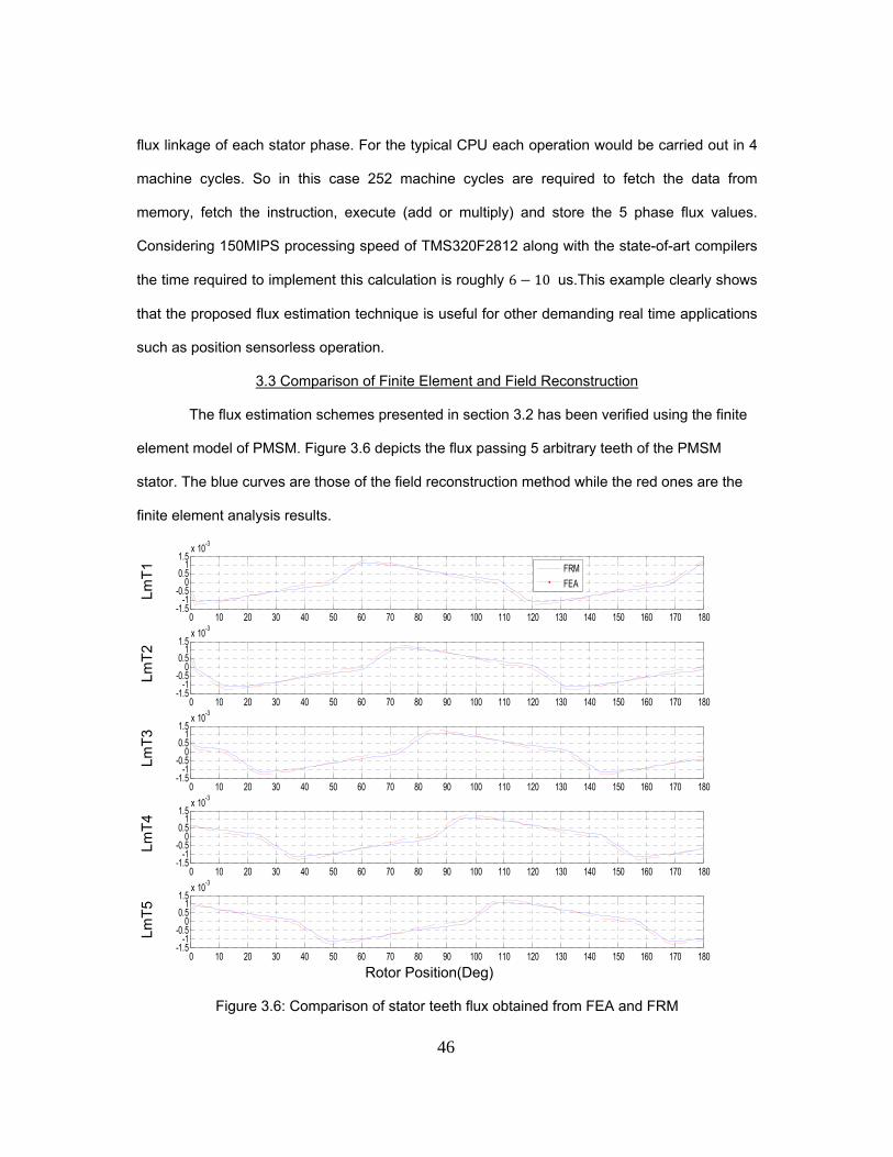
46

flux linkage of each stator phase. For the typical CPU each operation would be carried out in 4

machine cycles. So in this case 252 machine cycles are required to fetch the data from

memory, fetch the instruction, execute (add or multiply) and store the 5 phase flux values.

Considering 150MIPS processing speed of TMS320F2812 along with the state-of-art compilers

the time required to implement this calculation is roughly 6 10 us.This example clearly shows

that the proposed flux estimation technique is useful for other demanding real time applications

such as position sensorless operation.

3.3 Comparison of Finite Element and Field Reconstruction

The flux estimation schemes presented in section 3.2 has been verified using the finite

element model of PMSM. Figure 3.6 depicts the flux passing 5 arbitrary teeth of the PMSM

stator. The blue curves are those of the field reconstruction method while the red ones are the

finite element analysis results.

LmT

1

LmT

2 Lm

T3

LmT

4 Lm

T5

Rotor Position(Deg)

Figure 3.6: Comparison of stator teeth flux obtained from FEA and FRM

0 10 20 30 40 50 60 70 80 90 100 110 120 130 140 150 160 170 180-1.5

-1-0.5

00.5

11.5

x 10-3

0 10 20 30 40 50 60 70 80 90 100 110 120 130 140 150 160 170 180-1.5

-1-0.5

00.5

11.5

x 10-3

0 10 20 30 40 50 60 70 80 90 100 110 120 130 140 150 160 170 180-1.5

-1-0.5

00.5

11.5

x 10-3

0 10 20 30 40 50 60 70 80 90 100 110 120 130 140 150 160 170 180-1.5

-1-0.5

00.5

11.5

x 10-3

0 10 20 30 40 50 60 70 80 90 100 110 120 130 140 150 160 170 180-1.5

-1-0.5

00.5

11.5

x 10-3

FRM

FEA

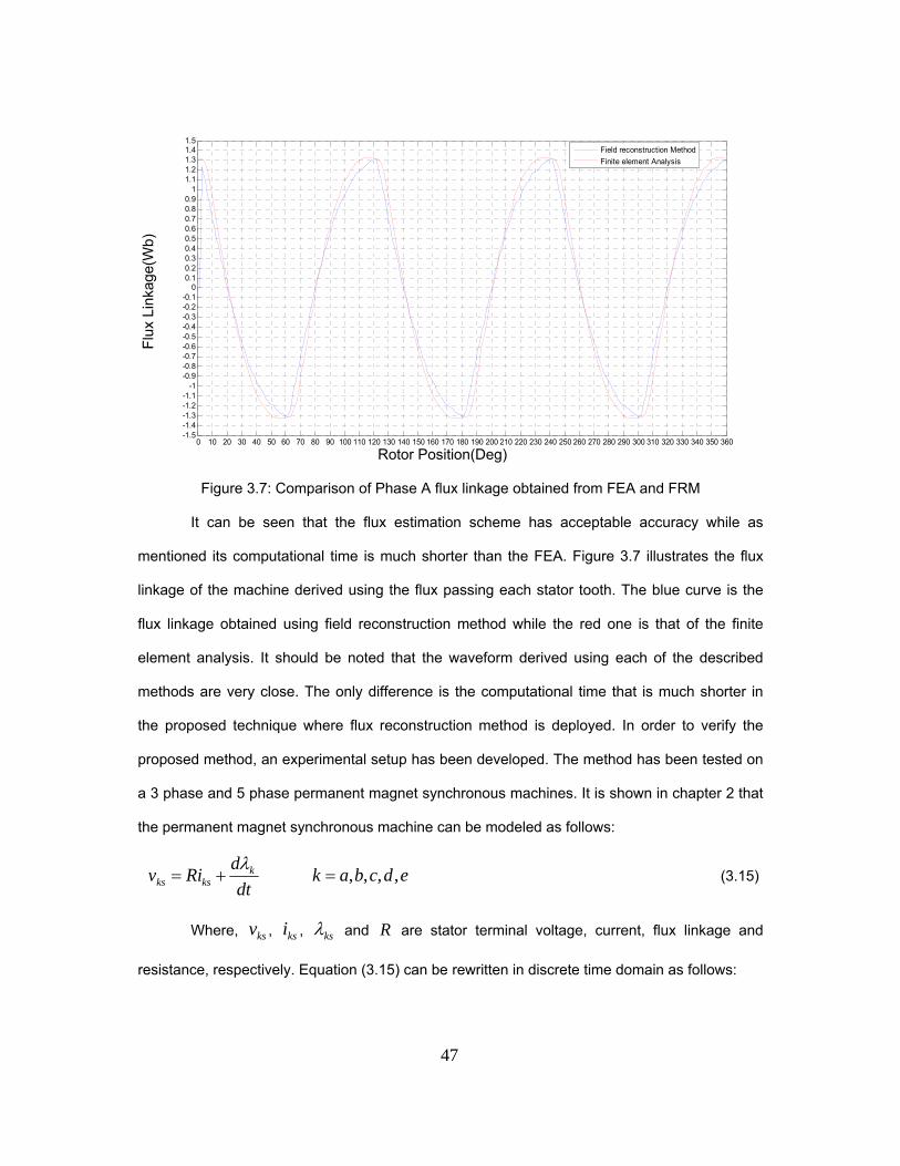
47

Flu

x Li

nkag

e(W

b)

Rotor Position(Deg)

Figure 3.7: Comparison of Phase A flux linkage obtained from FEA and FRM

It can be seen that the flux estimation scheme has acceptable accuracy while as

mentioned its computational time is much shorter than the FEA. Figure 3.7 illustrates the flux

linkage of the machine derived using the flux passing each stator tooth. The blue curve is the

flux linkage obtained using field reconstruction method while the red one is that of the finite

element analysis. It should be noted that the waveform derived using each of the described

methods are very close. The only difference is the computational time that is much shorter in

the proposed technique where flux reconstruction method is deployed. In order to verify the

proposed method, an experimental setup has been developed. The method has been tested on

a 3 phase and 5 phase permanent magnet synchronous machines. It is shown in chapter 2 that

the permanent magnet synchronous machine can be modeled as follows:

edcbakdt

dRiv k

ksks ,,,,

(3.15)

Where, ksv , ksi , ks and R are stator terminal voltage, current, flux linkage and

resistance, respectively. Equation (3.15) can be rewritten in discrete time domain as follows:

0 10 20 30 40 50 60 70 80 90 100 110 120 130 140 150 160 170 180 190 200 210 220 230 240 250 260 270 280 290 300 310 320 330 340 350 360-1.5-1.4-1.3-1.2-1.1

-1-0.9-0.8-0.7-0.6-0.5-0.4-0.3-0.2-0.1

00.10.20.30.40.50.60.70.80.9

11.11.21.31.41.5

Field reconstruction Method

Finite element Analysis

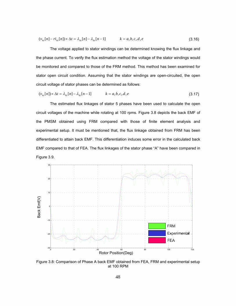
48

edcbaknntnrinv ksksksks ,,.,,]1[][])[][( (3.16)

The voltage applied to stator windings can be determined knowing the flux linkage and

the phase current. To verify the flux estimation method the voltage of the stator windings would

be monitored and compared to those of the FRM method. This method has been examined for

stator open circuit condition. Assuming that the stator windings are open-circuited, the open

circuit voltage of stator phases can be determined as follows:

edcbaknntnv ksksks ,,.,,]1[][])[( (3.17)

The estimated flux linkages of stator 5 phases have been used to calculate the open

circuit voltages of the machine while rotating at 100 rpms. Figure 3.8 depicts the back EMF of

the PMSM obtained using FRM compared with those of finite element analysis and

experimental setup. It must be mentioned that, the flux linkage obtained from FRM has been

differentiated to attain back EMF. This differentiation induces some error in the calculated back

EMF compared to that of FEA. The flux linkages of the stator phase “A” have been compared in

Figure 3.9.

Bac

k E

mf(

V)

0 20 40 60 80 100 120-30

-20

-10

0

10

20

30

Rotor Position(Deg)

Figure 3.8: Comparison of Phase A back EMF obtained from FEA, FRM and experimental setup at 100 RPM

49

Flu

x lin

kage

(Wb)

0 20 40 60 80 100 120-1.5

-1

-0.5

0

0.5

1

1.5

Rotor Position(Deg)

Figure 3.9: Comparison of Phase “A: flux linkage obtained from FEA, FRM and experimental setup at 100 RPM

To obtain the actual flux linkage, the measured terminal volateg is integrated. The

comparison of the results validates the accuracy of the flux linkage values calculated using the

flux estimator. The flux estimator is also tested on the 3 phase setup at REVT. The

experimental setup is shown in Figure 3.10. Equations 3.15 – 3.17 can be rewritten for 3-phase

PMSM as follows:

cbakdt

dRiv k

ksks ,,

(3.18)

cbaknntnrinv ksksksks ,,]1[][])[][(

(3.19)

cbaknntnv ksksks ,,]1[][])[(

(3.20)

The estimated flux linkages of stator 3 phases have been used to calculate the open

circuit voltages of the machine while rotating at 1000 rpm. Figures 3.11 and 3.12 depict the

back EMF of the PMSM obtained using FRM and experimental setup respectively. The back

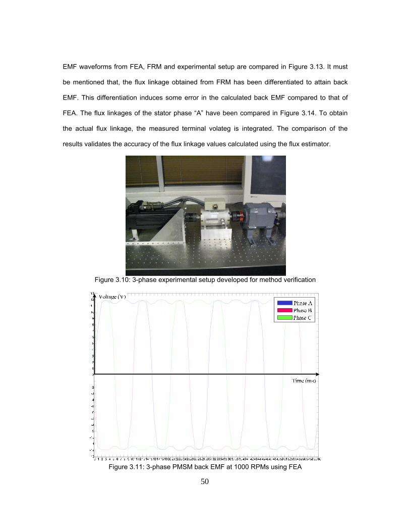
50

EMF waveforms from FEA, FRM and experimental setup are compared in Figure 3.13. It must

be mentioned that, the flux linkage obtained from FRM has been differentiated to attain back

EMF. This differentiation induces some error in the calculated back EMF compared to that of

FEA. The flux linkages of the stator phase “A” have been compared in Figure 3.14. To obtain

the actual flux linkage, the measured terminal volateg is integrated. The comparison of the

results validates the accuracy of the flux linkage values calculated using the flux estimator.

Figure 3.10: 3-phase experimental setup developed for method verification

Figure 3.11: 3-phase PMSM back EMF at 1000 RPMs using FEA

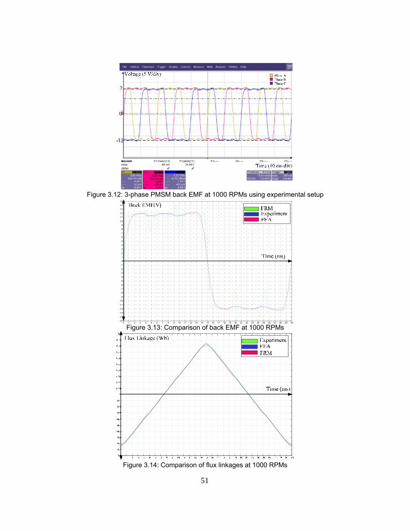
51

Figure 3.12: 3-phase PMSM back EMF at 1000 RPMs using experimental setup

0 1 2 3 4 5 6 7 8 9 10 11 12 13 14 15 16 17 18 19 20 21 22 23 24 25 26 27 28 29 30-15

-14

-13

-12

-11

-10

-9

-8

-7

-6

-5

-4

-3

-2

-1

0

1

2

3

4

5

6

7

8

9

10

11

12

13

14

15

Figure 3.13: Comparison of back EMF at 1000 RPMs

Figure 3.14: Comparison of flux linkages at 1000 RPMs

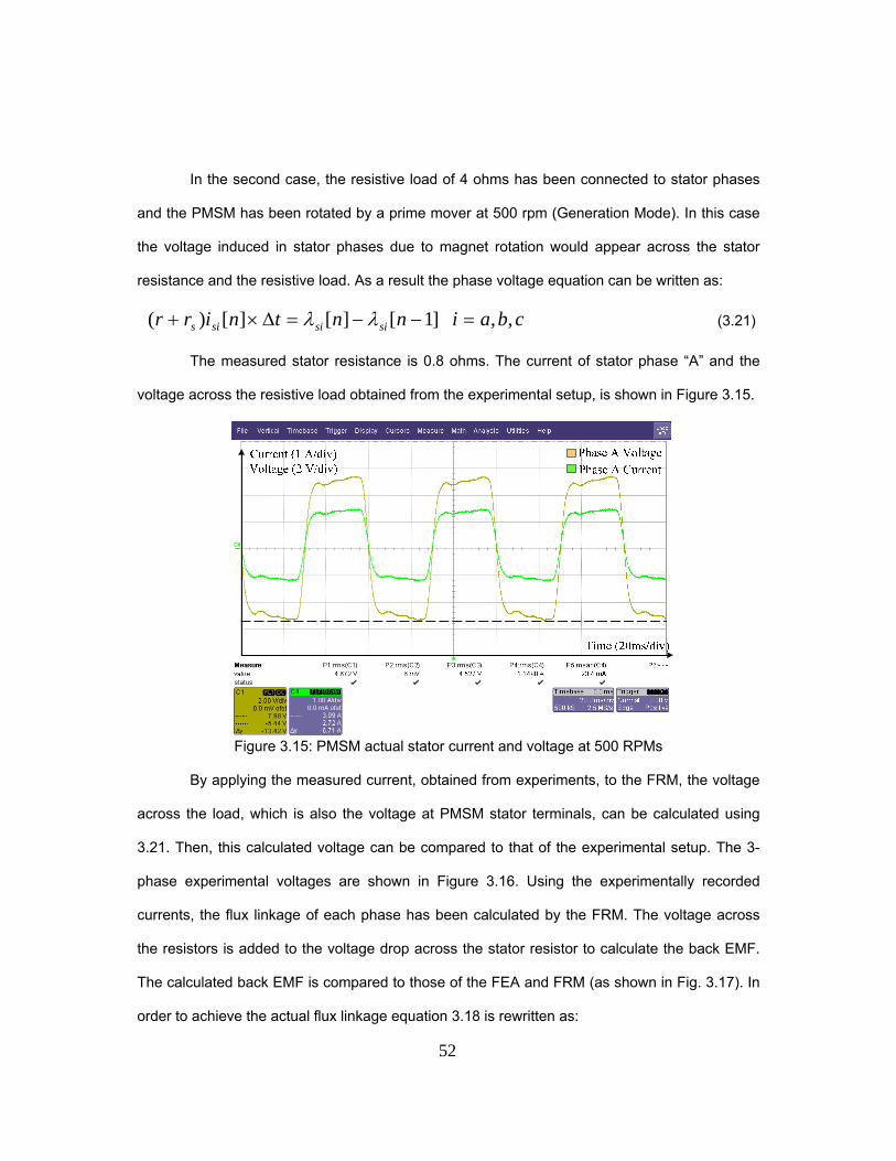
52

In the second case, the resistive load of 4 ohms has been connected to stator phases

and the PMSM has been rotated by a prime mover at 500 rpm (Generation Mode). In this case

the voltage induced in stator phases due to magnet rotation would appear across the stator

resistance and the resistive load. As a result the phase voltage equation can be written as:

cbainntnirr sisisis ,,]1[][][)( (3.21)

The measured stator resistance is 0.8 ohms. The current of stator phase “A” and the

voltage across the resistive load obtained from the experimental setup, is shown in Figure 3.15.

Figure 3.15: PMSM actual stator current and voltage at 500 RPMs

By applying the measured current, obtained from experiments, to the FRM, the voltage

across the load, which is also the voltage at PMSM stator terminals, can be calculated using

3.21. Then, this calculated voltage can be compared to that of the experimental setup. The 3-

phase experimental voltages are shown in Figure 3.16. Using the experimentally recorded

currents, the flux linkage of each phase has been calculated by the FRM. The voltage across

the resistors is added to the voltage drop across the stator resistor to calculate the back EMF.

The calculated back EMF is compared to those of the FEA and FRM (as shown in Fig. 3.17). In

order to achieve the actual flux linkage equation 3.18 is rewritten as:

53

cbaidtriv ksksks ,,)( (3.22)

The flux linkage of phase “A” obtained from FRM is compared to those of FEA and

experimental in Figure 3.17. It should be mentioned that equation 3.22 has been used here only

to compare the results. The flux observer can calculate the back EMF accurately, except for the

notches which represent stator slots. This error can be alleviated by using more accurate basis

functions in FRM code. Also, indirect comparison using differentiation may induce some error in

the measured quantities.

Figure 3.16: PMSM stator terminal voltages (Generation Mode)

1 2 3 4 5 6 7 8 9 10 111213 141516 171819 202122 232425 262728 293031 323334 353637 38 39 40 414243 444546 474849 505152 535455 565758 5960-8

-7

-6

-5

-4

-3

-2

-1

0

1

2

3

4

5

6

7

8

Figure 3.17: Comparison of back EMF at 500 RPMs (Generation Mode)

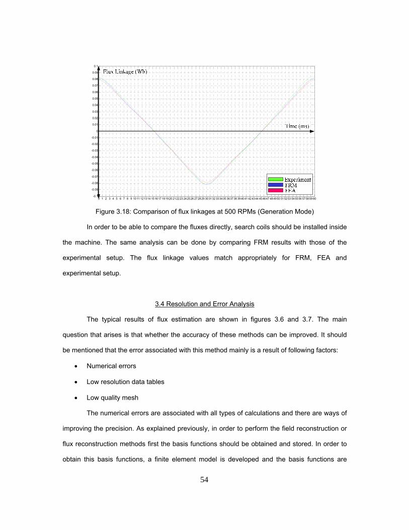
54

0 1 2 3 4 5 6 7 8 9 1011 1213 14 15 16 17 18 1920 212223 2425 26 27 28 29 30 3132 333435 3637 38 39 40 41 42 4344 454647 484950 5152 53 54 5556 575859 60-0.1

-0.09

-0.08

-0.07

-0.06

-0.05

-0.04

-0.03

-0.02

-0.01

0

0.01

0.02

0.03

0.04

0.05

0.06

0.07

0.08

0.09

0.1

Figure 3.18: Comparison of flux linkages at 500 RPMs (Generation Mode)

In order to be able to compare the fluxes directly, search coils should be installed inside

the machine. The same analysis can be done by comparing FRM results with those of the

experimental setup. The flux linkage values match appropriately for FRM, FEA and

experimental setup.

3.4 Resolution and Error Analysis

The typical results of flux estimation are shown in figures 3.6 and 3.7. The main

question that arises is that whether the accuracy of these methods can be improved. It should

be mentioned that the error associated with this method mainly is a result of following factors:

Numerical errors

Low resolution data tables

Low quality mesh

The numerical errors are associated with all types of calculations and there are ways of

improving the precision. As explained previously, in order to perform the field reconstruction or

flux reconstruction methods first the basis functions should be obtained and stored. In order to

obtain this basis functions, a finite element model is developed and the basis functions are

55

derived. If high resolution mesh is deployed in this process, the resulting basis function will be

more accurate. However, a denser mesh means a longer simulation time which is not always

desirable. Another factor that affects the accuracy is the number of points being stored in the

data tables of basis functions. This resolution can vary between a few samples per degree to a

sample per multiple degrees. Therefore, by increasing the mesh density the accuracy of basis

functions is guaranteed while having high resolution in basis functions improves the estimation

accuracy. The accuracy of the current measurements using current sensors is another factor

that affects the quality of the basis functions.

56

CHAPTER 4

FAULT TOLERANT OPERATION IN PMSM

The present chapter introduces various types of faults that can occur in an adjustable

speed PMSM drive, their methods of detection, clearance and treatment.

4.1 Classification of Faults in PMSM

Generally, the most frequently occuring faults in the permanent magnet motor drive can

be classified into the following categories:

Faults related to electrical structure

Faults related to mechanical structure

As mentioned before a multi phase drive, in which each phase is regarded as a single

module is the best design for fault tolerant purposes (increasing redundancy). These modules

should have the minimal impact on each other so that the failure in one does not affect the

others. The modular approach requires:

Separate single phase bridges (Minimal electrical interaction).

In case of the magnetic coupling between the phases, fault current in one can induce

voltages in the remaining phases, which in turn causes problems especially in the

control process (Minimal magnetic interaction).

The stator outer surface should be cooled down properly (Minimal thermal interaction).

To achieve the above mentioned goals the PMSM should be excited using separate full

bridges per each phase. In this case if any of the stator phases or their corresponding power

electronics experience a fault it can be disengaged from the healthy components. Based on this

arrangement the faults possible on the power electronics components and electrical machine

phases can be illustrated as shown in Figure 4.1.

57

Figure 4.1: Full bridge converter for one phase of PMSM

According to figure 4.1 the faults can be classified into the following:

Short and open circuit faults on the DC link (1)

Short and open circuit faults on switches (2, 4, 8, 10)

Short and open circuit faults on the diodes (3, 5, 9, 11)

Open circuit fault on the machine phase winding (6)

Partial and complete short circuit faults on the machine phase sinding (7)

Besides these faults, there are a set of faults that can happen on the sensors

measuring current, voltage and position. These types of fault will undermine the control

accuracy and functionality. The second set of faults that can happen in an EMEC are from a

magnetic or mechnical nature. Among these faults, partial demagnetization of the rotor magnets

and static rotor shaft eccentricity has been considered here.

4.1.1 Open-circuit faults

The open circuit faults can either happen on the power electronics components or on

the machine stator windings. In case an open circuit happens in one or more of the phases.

Consequently, the current flowing into that phase will be zero. The open circuit faults will harm

performane of the machine in terms of magnetic field generation and distribution which results

58

in the loss of synchronism and torque. In this dissertation various types of the open circuits in

stator windings have been considered. The modeling of the machine would not be any different

from that of the healthy machine. In case an open circuit happens, the current corresponding to

that phase will zero in the field reconstruction model. Based on that the magnetic field

distribution and hence the flux linking each of the phases can be monitored for fault detection

purposes.

4.1.2 Rotor partial demagnetization

In case of a PMSM motor drive, besides the regular monitoring of the current and

voltage levels, maximum operating temperature is also limited due to the thermal limitations of

the permanent magnets and stator windings. This thermal limit can be exceeded due to poor

ventilation (excessive heat) or excessive currents (extreme magnetic field) caused by short

circuits. These would change the magnetic properties of the permanent magnets resulting in

potential demagnetization. This demagnetization will affect the performance of the machine by a

great extent. The demagnetization of the magnets can be classified into the following:

Thermal shock [49]

Mechanical shock [49]

Magnetic shock [50]

The permanent magnet can maintain its properties as long as its temperature is within

the safe range. In the case of some faults such as short circuit, or overheating due to poor

cooling, the temperature of the PM machine increases and can result in partial demagnetization.

In this case a degradation of the coercive force of the permanent magnet can occur. As

discussed in [50], variation of temperature can degrade the performance of permanent

magnets. Also, mechanical shock can partially or totally damage the permanent magnets.

Magnet degradation, especially for Nd-Fe-B permanent magnets, can occur in case of inclined

field which normally leads to a phase displacement between the magnetization direction of the

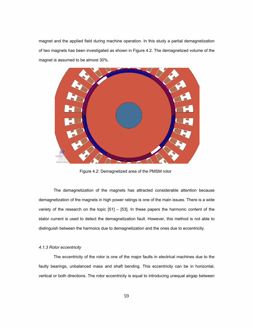
59

magnet and the applied field during machine operation. In this study a partial demagnetization

of two magnets has been investigated as shown in Figure 4.2. The demagnetized volume of the

magnet is assumed to be almost 30%.

Figure 4.2: Demagnetized area of the PMSM rotor

The demagnetization of the magnets has attracted considerable attention because

demagnetization of the magnets in high power ratings is one of the main issues. There is a wide

variety of the research on the topic [51] – [53]. In these papers the harmonic content of the

stator current is used to detect the demagnetization fault. However, this method is not able to

distinguish between the harmoics due to demagnetization and the ones due to eccentricity.

4.1.3 Rotor eccentricity

The eccentricity of the rotor is one of the major faults in electrical machines due to the

faulty bearings, unbalanced mass and shaft bending. This eccentricity can be in horizontal,

vertical or both directions. The rotor eccentricity is equal to introducing unequal airgap between

60

the stator and the rotor that causes an asymmetric distribution of the magnetic field in the

airgap. The eccentricity of the rotor can be classified into the following categories:

Static eccentricity

Dynamic eccentricity

In case of a static eccentricity, the position of minimal radial airgap length is constant

during the rotation of the rotor meaning that the rotor is shifted towards one side but it does not

move during rotation. In the case of static eccentricity, the amplitude of the forces exerting on

the stator teeth would alter and result in unbalanced radial forces. This can cause magnetic and

dynamic issues resulting in vibrations, noises and torque pulsations. There are various methods

of eccentricity fault detection, such as current spectrum analysis [54].

Figure 4.3: Eccentric 5-phase PMSM

In case of a dynamic ecentricity, the center of the shaft is eccentric and the airgap

changes dynamically during rotation. In this dissertation, it is assumed that the rotor has 40%

61

static eccentricity in horizontal direction as shown in Figure 4.3. It means that the center of the

shaft is replaced by 40% of the airgap length in horizontal direction.

4.2 FRM modeling of the Faulty machine

As described in the previous chapters a finite element model should be developed to

analyze the behavior of the machine under healthy and faulty operations. It has been shown

that to develop a comprehensive model for the PMSM, the basis functions and PM contribution

to the magnetic field components should be measured and stored. The process of obtaining the

basis functions and PM contribution has been described in section 2.1.

In case of a fault in the PMSM, the arrangement of the machine components would be

lost or at least altered compared with the healthy case. So, the basis functions and/or PM

contribution should be modified and replaced by the ones that include the fault impact. For

example, in case of the rotor permanent magnet partial demagnetization, the PM contribution to

the magnetic field is altered because of the change in the magnetic properties of the PMs on the

rotor.

4.2.1 FRM modeling of partial demagetization

In this study, the demagnetized volume of the magnet is assumed to be almost 15%. To

achieve the radial and tangential components of the magnetic field, the FR model should be

modified to comply with the changes made, to account for the demagnetized volume of the

permanent magnets. In case of demagnetization the PM contribution to the magnetic field is

different from that of the healthy machine, so the magnetic field distribution due to the magnets

should be captured and used instead of the healthy PM contribution.

Figure 4.4 illustrates the PM contribution to the magnetic field for healthy case and

partially demagnetized cases. In case of demagnetization, the corresponding data would be

used instead of the healthy case data.

62

Bn(

T)

0 60 120 180 240 300 360-0.4

-0.3

-0.2

-0.1

0

0.1

0.2

0.3

0.4

Rotor Position(Deg)

(a)

Bt(

T)

0 60 120 180 240 300 36-0.15

-0.1

-0.05

0

0.05

0.1

0.15

Rotor Position(Deg)

(b) Figure 4.4: Demagnetization: PM contribution. (a) Normal (b) Tangential

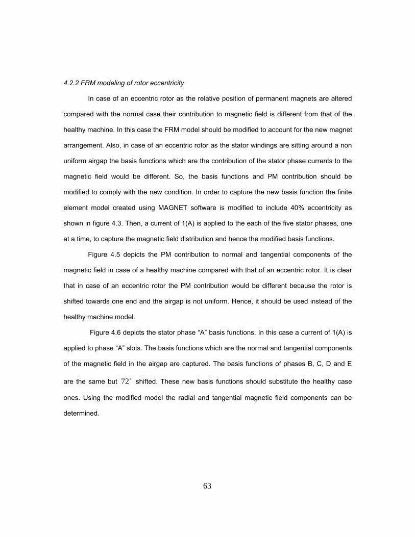
63

4.2.2 FRM modeling of rotor eccentricity

In case of an eccentric rotor as the relative position of permanent magnets are altered

compared with the normal case their contribution to magnetic field is different from that of the

healthy machine. In this case the FRM model should be modified to account for the new magnet

arrangement. Also, in case of an eccentric rotor as the stator windings are sitting around a non

uniform airgap the basis functions which are the contribution of the stator phase currents to the

magnetic field would be different. So, the basis functions and PM contribution should be

modified to comply with the new condition. In order to capture the new basis function the finite

element model created using MAGNET software is modified to include 40% eccentricity as

shown in figure 4.3. Then, a current of 1(A) is applied to the each of the five stator phases, one

at a time, to capture the magnetic field distribution and hence the modified basis functions.

Figure 4.5 depicts the PM contribution to normal and tangential components of the

magnetic field in case of a healthy machine compared with that of an eccentric rotor. It is clear

that in case of an eccentric rotor the PM contribution would be different because the rotor is

shifted towards one end and the airgap is not uniform. Hence, it should be used instead of the

healthy machine model.

Figure 4.6 depicts the stator phase “A” basis functions. In this case a current of 1(A) is

applied to phase “A” slots. The basis functions which are the normal and tangential components

of the magnetic field in the airgap are captured. The basis functions of phases B, C, D and E

are the same but 72 shifted. These new basis functions should substitute the healthy case

ones. Using the modified model the radial and tangential magnetic field components can be

determined.

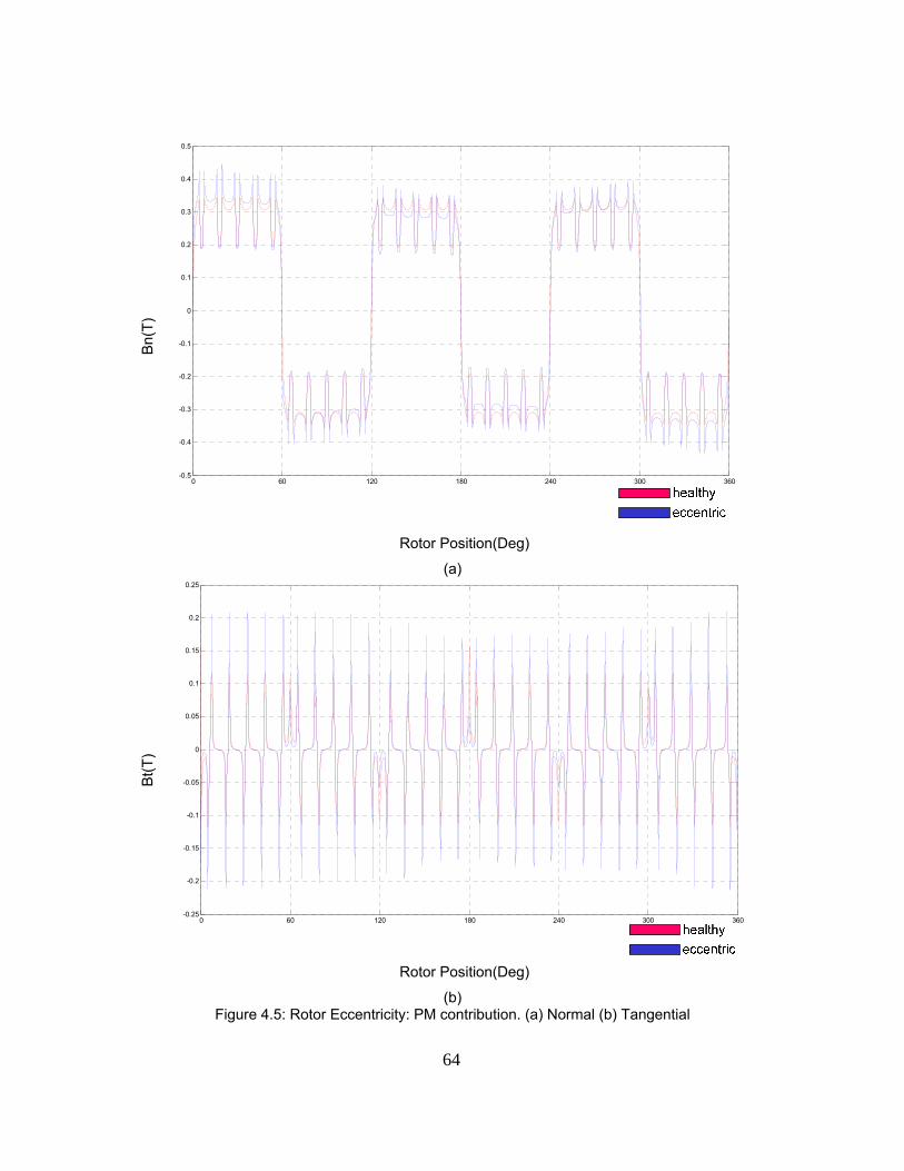
64

Bn(

T)

0 60 120 180 240 300 360-0.5

-0.4

-0.3

-0.2

-0.1

0

0.1

0.2

0.3

0.4

0.5

Rotor Position(Deg)

(a)

Bt(

T)

0 60 120 180 240 300 360-0.25

-0.2

-0.15

-0.1

-0.05

0

0.05

0.1

0.15

0.2

0.25

Rotor Position(Deg)

(b) Figure 4.5: Rotor Eccentricity: PM contribution. (a) Normal (b) Tangential

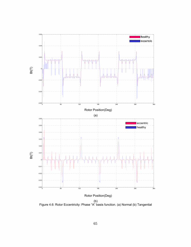
65

B

t(T

)

0 60 120 180 240 300 360-0.06

-0.04

-0.02

0

0.02

0.04

0.06

Rotor Position(Deg)

(a)

Bt(

T)

0 60 120 180 240 300 360-0.04

-0.03

-0.02

-0.01

0

0.01

0.02

0.03

0.04

0.05

0.06

eccentric

healthy

Rotor Position(Deg)

(b) Figure 4.6: Rotor Eccentricity: Phase “A” basis function. (a) Normal (b) Tangential

66

4.3 Fault detection Using FRM

In this dissertation a combination of the flux based and current based techniques has

been considered to detect the fault. This technique includes the injection of the measured

currents into the field reconstruction module and detrmination of the flux linkages due to that

current and then comparison of the resulting fluxes with those of the healthy machine. In case of

not matching flux linkages, the flux linkage can be investigated to determine the type of the

fault. The fault detection scheme has been depicted in figure 4.7. The detection signatures for

each type of fault and the treatment to obtain maximum average torque have been presented in

the following sections.

,... 5.1 ii

tn BB ,

51...

*5

*1 ...

Figure 4.7: Fault detection flowchart

4.3.1 Open-circuit fault detection

The electrical power is supplied to the machine through the stator phases. Loss of any

of phases would result in lower input power to the motor and hence the output torque would be

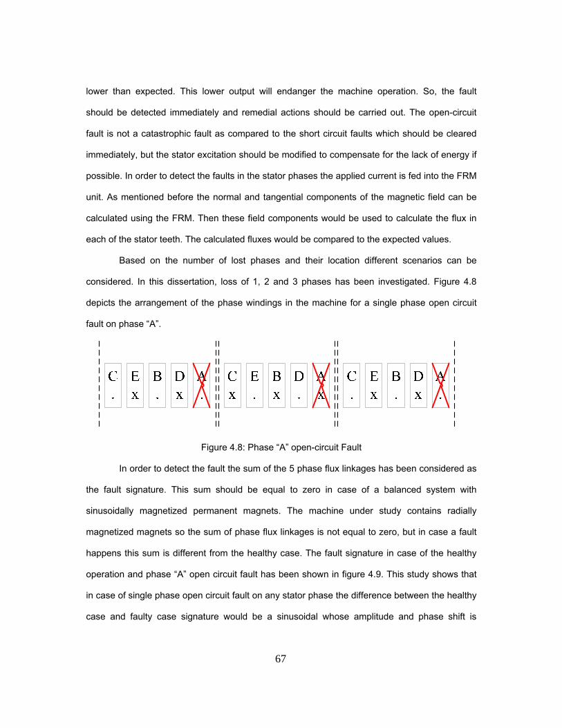
67

lower than expected. This lower output will endanger the machine operation. So, the fault

should be detected immediately and remedial actions should be carried out. The open-circuit

fault is not a catastrophic fault as compared to the short circuit faults which should be cleared

immediately, but the stator excitation should be modified to compensate for the lack of energy if

possible. In order to detect the faults in the stator phases the applied current is fed into the FRM

unit. As mentioned before the normal and tangential components of the magnetic field can be

calculated using the FRM. Then these field components would be used to calculate the flux in

each of the stator teeth. The calculated fluxes would be compared to the expected values.

Based on the number of lost phases and their location different scenarios can be

considered. In this dissertation, loss of 1, 2 and 3 phases has been investigated. Figure 4.8

depicts the arrangement of the phase windings in the machine for a single phase open circuit

fault on phase “A”.

Figure 4.8: Phase “A” open-circuit Fault

In order to detect the fault the sum of the 5 phase flux linkages has been considered as

the fault signature. This sum should be equal to zero in case of a balanced system with

sinusoidally magnetized permanent magnets. The machine under study contains radially

magnetized magnets so the sum of phase flux linkages is not equal to zero, but in case a fault

happens this sum is different from the healthy case. The fault signature in case of the healthy

operation and phase “A” open circuit fault has been shown in figure 4.9. This study shows that

in case of single phase open circuit fault on any stator phase the difference between the healthy

case and faulty case signature would be a sinusoidal whose amplitude and phase shift is

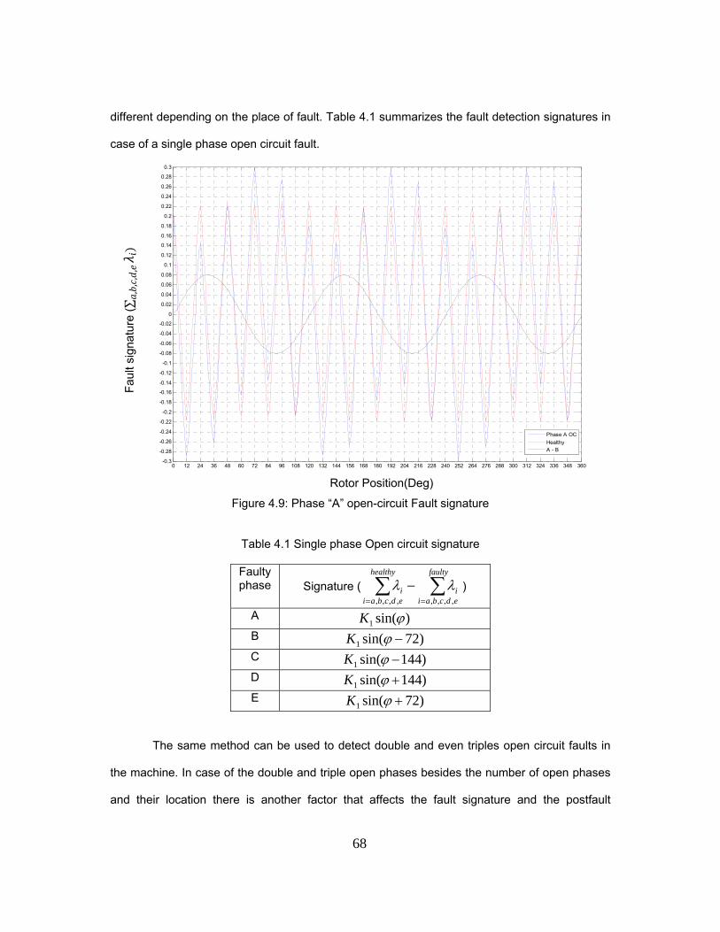
68

different depending on the place of fault. Table 4.1 summarizes the fault detection signatures in

case of a single phase open circuit fault. F

ault

sign

atur

e (∑

,,,,

Rotor Position(Deg)

Figure 4.9: Phase “A” open-circuit Fault signature

Table 4.1 Single phase Open circuit signature

Faulty phase Signature (

faulty

edcbaii

healthy

edcbaii

,,,,,,,,

)

A )sin(1 K

B )72sin(1 K

C )144sin(1 K

D )144sin(1 K

E )72sin(1 K

The same method can be used to detect double and even triples open circuit faults in

the machine. In case of the double and triple open phases besides the number of open phases

and their location there is another factor that affects the fault signature and the postfault

0 12 24 36 48 60 72 84 96 108 120 132 144 156 168 180 192 204 216 228 240 252 264 276 288 300 312 324 336 348 360-0.3

-0.28

-0.26

-0.24

-0.22

-0.2

-0.18

-0.16

-0.14

-0.12

-0.1

-0.08

-0.06

-0.04

-0.02

0

0.02

0.04

0.06

0.08

0.1

0.12

0.14

0.16

0.18

0.2

0.22

0.24

0.26

0.28

0.3

Phase A OC

HealthyA - B

69

treatment scheme. It is important whether adjacent or nonadjacent phases are missing. Figure

4.10 depicts the case of an adjacent open circuit fault on phases “A” and “C”.

(a)

Fau

lt si

gnat

ure

(∑,,,,

Rotor Position(Deg) (b)

Figure 4.10: Adjacent double open circuit (a) Winding arrangement, (b) Fault signature.

In case of a non-adjacent double open circuit the signature will be different from that of

the adjacent case. Figure 4.11 depicts the winding arrangement and fault signature for this

case. In this figure, the sum of the flux linkages for healthy and faulty cases has been presented

with blue and red curves, respetively. Table 4.2 summarizes the fault detection signatures in

case of an adjacent or non-adjacent double phase open circuit fault. According to the table, the

0 12 24 36 48 60 72 84 96 108 120 132 144 156 168 180 192 204 216 228 240 252 264 276 288 300 312 324 336 348 360-0.4

-0.38

-0.36

-0.34

-0.32

-0.3

-0.28

-0.26

-0.24

-0.22

-0.2

-0.18

-0.16

-0.14

-0.12

-0.1

-0.08

-0.06

-0.04

-0.02

0

0.02

0.04

0.06

0.08

0.1

0.12

0.14

0.16

0.18

0.2

0.22

0.24

0.26

0.28

0.3

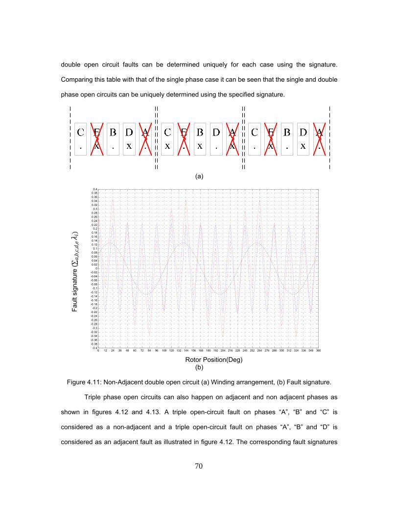
70

double open circuit faults can be determined uniquely for each case using the signature.

Comparing this table with that of the single phase case it can be seen that the single and double

phase open circuits can be uniquely determined using the specified signature.

(a)

Fau

lt si

gnat

ure

(∑,,,,

Rotor Position(Deg) (b)

Figure 4.11: Non-Adjacent double open circuit (a) Winding arrangement, (b) Fault signature.

Triple phase open circuits can also happen on adjacent and non adjacent phases as

shown in figures 4.12 and 4.13. A triple open-circuit fault on phases “A”, “B” and “C” is

considered as a non-adjacent and a triple open-circuit fault on phases “A”, “B” and “D” is

considered as an adjacent fault as illustrated in figure 4.12. The corresponding fault signatures

0 12 24 36 48 60 72 84 96 108 120 132 144 156 168 180 192 204 216 228 240 252 264 276 288 300 312 324 336 348 360-0.4

-0.38-0.36-0.34-0.32-0.3

-0.28-0.26-0.24-0.22-0.2

-0.18-0.16-0.14-0.12-0.1

-0.08-0.06-0.04-0.02

00.020.040.060.080.1

0.120.140.160.180.2

0.220.240.260.280.3

0.320.340.360.380.4

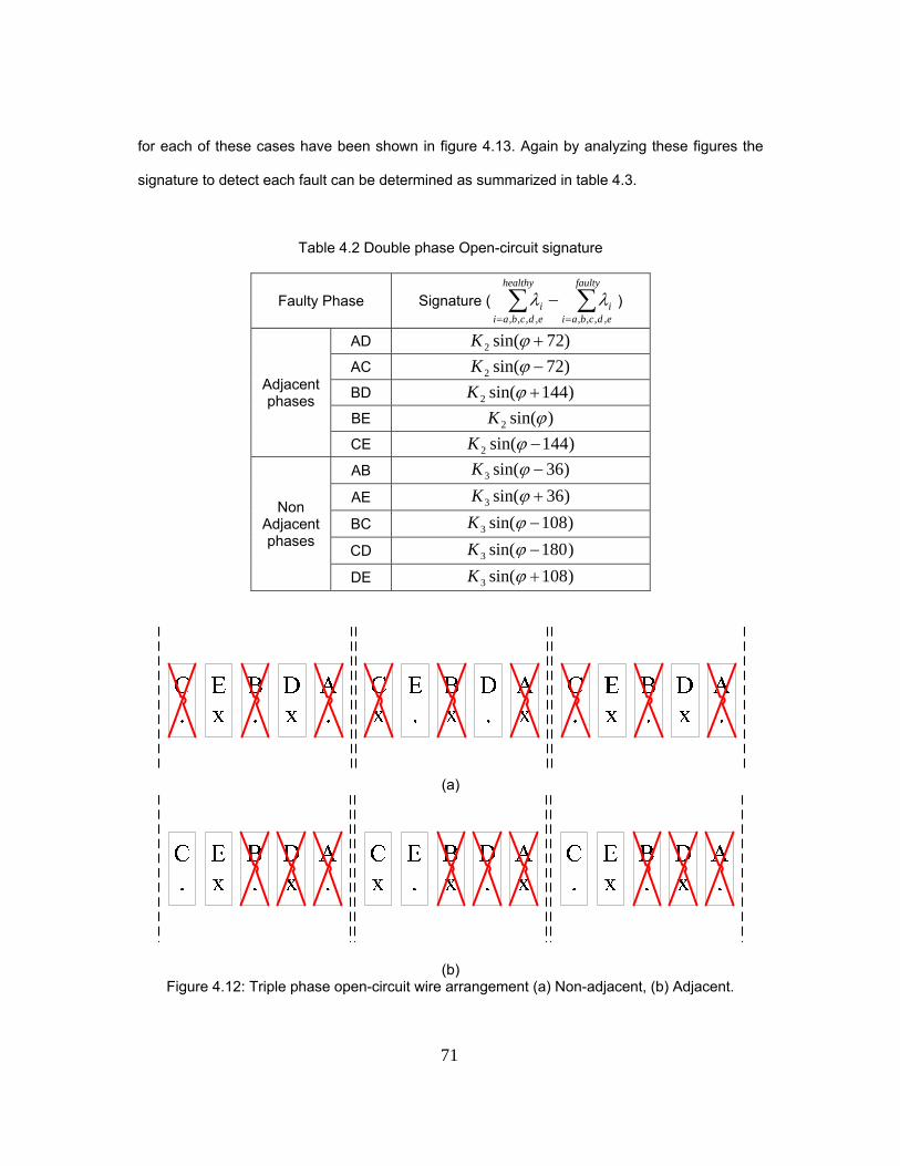
71

for each of these cases have been shown in figure 4.13. Again by analyzing these figures the

signature to detect each fault can be determined as summarized in table 4.3.

Table 4.2 Double phase Open-circuit signature

Faulty Phase Signature (

faulty

edcbaii

healthy

edcbaii

,,,,,,,,

)

Adjacent phases

AD )72sin(2 K

AC )72sin(2 K

BD )144sin(2 K

BE )sin(2 K

CE )144sin(2 K

Non Adjacent phases

AB )36sin(3 K

AE )36sin(3 K

BC )108sin(3 K

CD )180sin(3 K

DE )108sin(3 K

(a)

(b)

Figure 4.12: Triple phase open-circuit wire arrangement (a) Non-adjacent, (b) Adjacent.

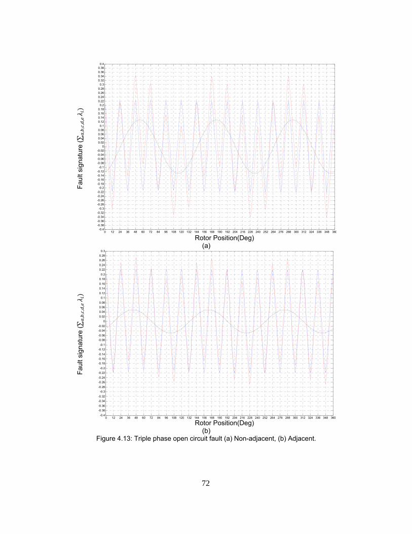
72

Fau

lt si

gnat

ure

(∑,,,,

Rotor Position(Deg) (a)

Fau

lt si

gnat

ure

(∑,,,,

Rotor Position(Deg) (b)

Figure 4.13: Triple phase open circuit fault (a) Non-adjacent, (b) Adjacent.

0 12 24 36 48 60 72 84 96 108 120 132 144 156 168 180 192 204 216 228 240 252 264 276 288 300 312 324 336 348 360-0.4

-0.38-0.36-0.34-0.32-0.3

-0.28-0.26-0.24-0.22-0.2

-0.18-0.16-0.14-0.12-0.1

-0.08-0.06-0.04-0.02

00.020.040.060.080.1

0.120.140.160.180.2

0.220.240.260.280.3

0.320.340.360.380.4

0 12 24 36 48 60 72 84 96 108 120 132 144 156 168 180 192 204 216 228 240 252 264 276 288 300 312 324 336 348 360-0.4

-0.38

-0.36

-0.34

-0.32

-0.3

-0.28

-0.26

-0.24

-0.22

-0.2

-0.18

-0.16

-0.14

-0.12

-0.1

-0.08

-0.06

-0.04

-0.02

0

0.02

0.04

0.06

0.08

0.1

0.12

0.14

0.16

0.18

0.2

0.22

0.24

0.26

0.28

0.3

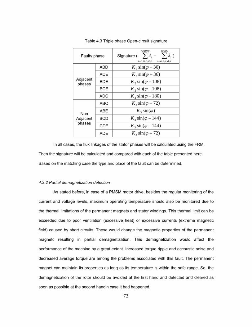
73

Table 4.3 Triple phase Open-circuit signature

Faulty phase Signature (

faulty

edcbaii

healthy

edcbaii

,,,,,,,,

)

Adjacent phases

ABD )36sin(2 K

ACE )36sin(2 K

BDE )108sin(2 K

BCE )108sin(2 K

ADC )180sin(2 K

Non Adjacent phases

ABC )72sin(3 K

ABE )sin(3 K

BCD )144sin(3 K

CDE )144sin(3 K

ADE )72sin(3 K

In all cases, the flux linkages of the stator phases will be calculated using the FRM.

Then the signature will be calculated and compared with each of the table presented here.

Based on the matching case the type and place of the fault can be determined.

4.3.2 Partial demagnetization detection

As stated before, in case of a PMSM motor drive, besides the regular monitoring of the

current and voltage levels, maximum operating temperature should also be monitored due to

the thermal limitations of the permanent magnets and stator windings. This thermal limit can be

exceeded due to poor ventilation (excessive heat) or excessive currents (extreme magnetic

field) caused by short circuits. These would change the magnetic properties of the permanent

magnetc resulting in partial demagnetization. This demagnetization would affect the

performance of the machine by a great extent. Increased torque ripple and accoustic noise and

decreased average torque are among the problems associated with this fault. The permanent

magnet can maintain its properties as long as its temperature is within the safe range. So, the

demagnetization of the rotor should be avoided at the first hand and detected and cleared as

soon as possible at the second handin case it had happened.

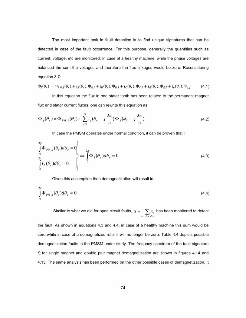
74

The most important task in fault detection is to find unique signatures that can be

detected in case of the fault occurrence. For this purpose, generally the quantities such as

current, voltage, etc are monitored. In case of a healthy machine, while the phase voltages are

balanced the sum the voltages and therefore the flux linkages would be zero. Reconsidering

equation 3.7:

Φ Φ , .Φ , .Φ , .Φ , .Φ , .Φ , (4.1)

In this equation the flux in one stator tooth has been related to the permanent magnet

flux and stator current fluxes, one can rewrite this equation as:

)5

2().

5

2()()(

5

1,

jji Sjej

jejPMej

(4.2)

In case the PMSM operates under normal condition, it can be proven that :

0)(

0)(

0)(2

02

0

2

0

,

eej

eeA

eejPM

d

di

d

(4.3)

Given this assumption then demagnetization will result in:

0)(2

0

, eejPM d

(4.4)

Similar to what we did for open circuit faults,

edcbaiiS

,,,,

has been monitored to detect

the fault. As shown in equations 4.3 and 4.4, in case of a healthy machine this sum would be

zero while in case of a demagnetized rotor it will no longer be zero. Table 4.4 depicts possible

demagnetization faults in the PMSM under study. The frequncy spectrum of the fault signature

S for single magnet and double pair magnet demagnetization are shown in figures 4.14 and

4.15. The same analysis has been performed on the other possible cases of demagnetization. It

75

is shown that in case of the rotor magnet demagnetization a set of frequencies would be

present in the FFT spectrum of S as summarized in Table 4.4.

Table 4.4: Demagnetization scenarios

Fault Scenario Place Frequencies to detect

Single magnet demagnetization N2

,....13.39

24.34

35.29

,46.24

56.19

67.14

78.9

89.4

8

7

6

5

4

3

2

1

f

f

f

f

f

f

f

f

S3

Double magnet demagnetization N1N2

S1S2

Triple magnet demagnetization N1N2N3

S1S2S3

2 Pair demagnetization N1N2S1S2

These frequencies could be used for detection purposes. According to the figures and

data from table and considering that the frequency of the stator sinusoidal current is known the

frequency spectrum could be determined using the following formula:

,.....3,2,12

kfP

kf edem (4.5)

Where, P and ef are the number of magnetic pole pairs and stator current frequency,

respectively. The magnetic flux density components will be calculated using field reconstruction

method for 1 electrical cycle. Then these components would be used to determine flux passing

each stator tooth which will finally be used to calculate the flux linkages of the stator phases.

Next step is to compare the expected flux linkage with the actual quantities. By applying the

FFT and low pass filtering the signature frequencies can be extracted.

76

S (

Wb)

Frequency (Hz)

Figure 4.14: Fault signature frequency spectrum. Single magnet demagnetization

S (

Wb)

Frequency (Hz)

Figure 4.15: Fault signature frequency spectrum. Double magnet pair demagnetization

0 20 40 60 80 100 120 140 160 180 200 220 240 260 280 300 320 340 360 380 400 420 440 460 480 5000

0.1

0.2

0.3

0.4

0.5

0.6

0.7

( )

N2

S3

0 20 40 60 80 100 120 140 160 180 200 220 240 260 280 300 320 340 360 380 400 420 440 460 480 5000

0.2

0.4

0.6

0.8

1

1.2

77

4.3.3 Rotor Eccentricity detection

In case of eccentricity as the rotor is closer to a set of windings the balance no longer

exists in the electrical quantities, so for the same amount of current applied as of the healthy

case some of the stator teeth would have higher levels of magnetic flux due to the proxomity to

the permanent magnets. Figure 4.16 depicts the comparison of the magnetic flux distribution in

the machine in case of a healthy machine and the one with an eccentric rotor. It can be seen

that the peak of magnetic flux is higher in case of eccentric rotor. Also, in case of eccentric rotor

the distribution of the magnetic flux around the airgap is no longer uniform. This signature can

be used to determine the eccentricity of the rotor. Similar to the partial demagnetization case, in

case of an eccentric rotor the magnetic flux can be written as:

0)()5

2().

5

2()()(

2

0

5

1,

eejSje

jjejPMej djji

(4.6)

This unbalance in the magnetic flux linking each stator phase can be used to detect the

eccentricity. The flux passing each stator tooth is measured using the FRM module and

compared with the flux for the healthy case and the unbalance of the flux shows the eccentricity

of the rotor. It should be mentioned that in case of an eccentric rotor there is no deformity in the

magnetic flux wavefrom as observed in case of PM demagnetization and the difference is in the

magitude of the flux. Figure 4.17 depicts the flux passing stator teeth in case of eccentric rotor

compared with the healthy machine. In this case an eccentricity of 30% has been considered for

the rotor.

78

(a)

(b) Figure 4.16: Magnetic flux distribution (a) healthy machine (b) eccentric rotor

79

0 60 120 180 240 300 360

-1

-0.8

-0.6

-0.4

-0.2

0

0.2

0.4

0.6

0.8

1

x 10-3

(a)

0 60 120 180 240 300 360-1.2

-1

-0.8

-0.6

-0.4

-0.2

0

0.2

0.4

0.6

0.8

1

1.2x 10

-3

(b)

Figure 4.17: Comparison of magnetic flux distribution (a) tooth#3 (b) tooth#20

4.4 Fault Treatment

Fault teartment is equally important as the fault detection in terms of machine

performance. Most of the research conducted on the fault detection is concentrated on the

methods of the fault detection. These valuable researches simply ignore what happens to the

system operation after the fault. Some of the fault tolerance methods suggest increasing the

redundancy of the system to compensate for the component loss in case of the fault. Although

80

helpful, increasing the redundancy of the system is not always possible because of the limitation

in the available space or due to the high price of the equivalent replacement device. On the

other hand increasing the redundancy leads in to a more complicated control strategy which

includes higher cost of control modules. In this dissertation the optimal excitation of the

remaining healthy components of the EMEC is considered as a survival technique to

compensate for the missing components.

The optimal currents for all the fault scenarios would be obtained and stored as

explaind later. In case the fault happens, based on the type and location of the fault the

appropriate set of currents would be applied to the PMSM stator phases to squeeze the

maximum torque possible. The optimization criteria can be changed based on the application.

Here the maximum average torque is considered while the torque ripple is minimized.

4.4.1 Open-circuit fault treatment

In most applications it is desirable to have the maximum output torque possible while

the torque ripple is minimized. This is not necessarily the most efficient way of running the

motor drive especially in terms of losses and harmonics. For example, considering the case of

the healthy 5 phase PMSM where no faults exist.

Normally, the sinusoidal excitation is used to drive the system because it introduces

fewer harmonics into the power electronics hardware hence reducing the losses and eliminating

the need to the filters. By the way, in applications where the maximum torque per RMS input

current is targeted sinusoidal excitation might not be the best choice. Figures 4.18 and 4.19

represent the sinusoidal and optimal excitation of the 5 phase PMSM machine.

To obtain the optimized waveforms the FRM code has been used in conjunction with

the MATLAB optimization toolbox. It can be seen that in case of the optimal excitation the

average output torque is higher than the case of the sinusoidal excitation as well as the torque

per ampere ratio. Table 4.5 depicts the numerical comparison of these two cases. Based on this

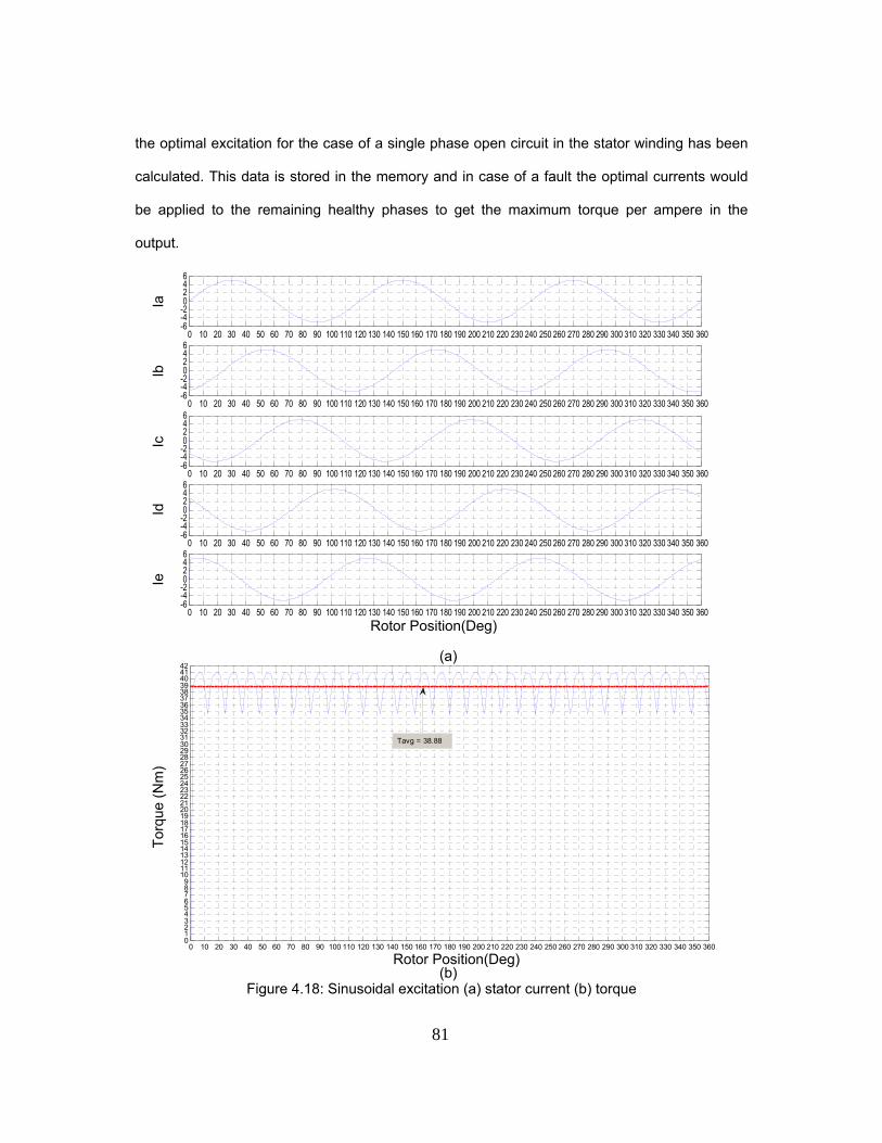
81

the optimal excitation for the case of a single phase open circuit in the stator winding has been

calculated. This data is stored in the memory and in case of a fault the optimal currents would

be applied to the remaining healthy phases to get the maximum torque per ampere in the

output.

Ia

Ib

Ic

Id

Ie

Rotor Position(Deg)

(a)

Tor

que

(Nm

)

Rotor Position(Deg) (b)

Figure 4.18: Sinusoidal excitation (a) stator current (b) torque

0 10 20 30 40 50 60 70 80 90 100 110 120 130 140 150 160 170 180 190 200 210 220 230 240 250 260 270 280 290 300 310 320 330 340 350 360-6-4-20246

0 10 20 30 40 50 60 70 80 90 100 110 120 130 140 150 160 170 180 190 200 210 220 230 240 250 260 270 280 290 300 310 320 330 340 350 360-6-4-20246

0 10 20 30 40 50 60 70 80 90 100 110 120 130 140 150 160 170 180 190 200 210 220 230 240 250 260 270 280 290 300 310 320 330 340 350 360-6-4-20246

0 10 20 30 40 50 60 70 80 90 100 110 120 130 140 150 160 170 180 190 200 210 220 230 240 250 260 270 280 290 300 310 320 330 340 350 360-6-4-20246

0 10 20 30 40 50 60 70 80 90 100 110 120 130 140 150 160 170 180 190 200 210 220 230 240 250 260 270 280 290 300 310 320 330 340 350 360-6-4-20246

0 10 20 30 40 50 60 70 80 90 100 110 120 130 140 150 160 170 180 190 200 210 220 230 240 250 260 270 280 290 300 310 320 330 340 350 3600123456789

101112131415161718192021222324252627282930313233343536373839404142

Tavg = 38.88

82

Ia

Ib

Ic

Id

Ie

Rotor Position(Deg) (a)

Tor

que

(Nm

)

Rotor Position(Deg) (b)

Figure 4.19: Optimal excitation (a) stator current (b) torque

Figure 4.20 depicts the optimal current waveforms in case of an open circuit fault in

phase “D”. Figure 4.21 depicts the resulting toque in case the optimized currents have been

applied to the remaining healthy phases. It can be seen that the average torque is decreased

0 20 40 60 80 100 120 140 160 180 200 220 240 260 280 300 320 340 360-6-4-20246

0 20 40 60 80 100 120 140 160 180 200 220 240 260 280 300 320 340 360-6-4-20246

0 20 40 60 80 100 120 140 160 180 200 220 240 260 280 300 320 340 360-6-4-20246

0 20 40 60 80 100 120 140 160 180 200 220 240 260 280 300 320 340 360-6-4-20246

0 20 40 60 80 100 120 140 160 180 200 220 240 260 280 300 320 340 360-6-4-20246

0 20 40 60 80 100 120 140 160 180 200 220 240 260 280 300 320 340 3600

2

46

810

12

1416

1820

2224

26

2830

3234

3638

40

4244

4648

5052

Tavg = 47.6976

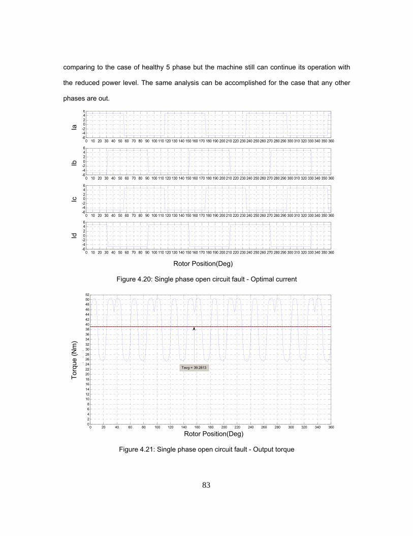
83

comparing to the case of healthy 5 phase but the machine still can continue its operation with

the reduced power level. The same analysis can be accomplished for the case that any other

phases are out.

Ia

Ib

Ic

Id

Rotor Position(Deg)

Figure 4.20: Single phase open circuit fault - Optimal current

Tor

que

(Nm

)

Rotor Position(Deg)

Figure 4.21: Single phase open circuit fault - Output torque

0 10 20 30 40 50 60 70 80 90 100 110 120 130 140 150 160 170 180 190 200 210 220 230 240 250 260 270 280 290 300 310 320 330 340 350 360-6-4-20246

0 10 20 30 40 50 60 70 80 90 100 110 120 130 140 150 160 170 180 190 200 210 220 230 240 250 260 270 280 290 300 310 320 330 340 350 360-6-4-20246

0 10 20 30 40 50 60 70 80 90 100 110 120 130 140 150 160 170 180 190 200 210 220 230 240 250 260 270 280 290 300 310 320 330 340 350 360-6-4-20246

0 10 20 30 40 50 60 70 80 90 100 110 120 130 140 150 160 170 180 190 200 210 220 230 240 250 260 270 280 290 300 310 320 330 340 350 360-6-4-20246

0 20 40 60 80 100 120 140 160 180 200 220 240 260 280 300 320 340 3600

24

68

101214

1618

2022

242628

3032

3436

384042

4446

485052

q(

)

Tavg = 39.2813

84

Table 4.5: Torque comparison for sinusoidal and optimal currents

Type of ExcitationrmsI

T

Sinusoidal 997.105355.388.38

rmsIT

Optimal 098.112979.46976.47

rmsIT

4.4.2 Partial demagnetization treatment

Depending on the service continuity strategy, various scenarios can be deployed after

the demagnetization fault is detected. In case, the service can be provided by another module

the machine could be stopped and the magnets being replaced. In case of an emergency

application in which service discontinuity is not possible the stator applied currents can be

modified in a way the maximum possible average torque could be squeezed out of the machine

shaft. Of course the presence of the harmonics in the current would result in extra torque

pulsations. For this purpose the field reconstruction method would be used in conjunction with

the optimization methods to attain the optimal current waveforms. Figure 4.22 depicts the output

mechanical torque of the machine for healthy and demagnetization fault cases in case

sinusoidal currents are applied to stator phases. It is shown that the average torque has

decreased almost 25% as a result of the magnet demagnetization. Also torque ripple has been

increased almost 30%. Using the optimization methods the optimal waveforms are determined

in case, demagnetization occurs. The Matlab optimization toolbox is linked to the FRM code.

For each rotor position, the optimization code calculates a set of currents based on the

optimization criteria. These currents are used to calculate the magnetic field components in the

machine. Then, using the magnetic field components the torque is calculated. In case the

calculated torque complies with the target values, the currents would be stored and a new rotor

85

position would be considered. Figure 4.23 depicts the optimal stator phase currents and the

output torque of the machine. T

orqu

e (N

m)

Rotor Position(Deg)

(a)

Tor

que

(Nm

)

Rotor Position(Deg)

(b)

Figure 4.22: Torque Analysis. (a) Healthy machine, (b) Partially demagnetized magnets

0 10 20 30 40 50 60 70 80 90 100 110 120 130 140 150 160 170 180 190 200 210 220 230 240 250 260 270 280 290 300 310 320 330 340 350 3600123456789

101112131415161718192021222324252627282930313233343536373839404142

Tavg = 38.88

0 10 20 30 40 50 60 70 80 90 100 110 120 130 140 150 160 170 180 190 200 210 220 230 240 250 260 270 280 290 300 310 320 330 340 350 3600

1

2

3

4

5

6

7

8

9

10

11

12

13

14

15

16

17

18

19

20

21

22

23

24

25

26

27

28

29

30

31

32

33

34

35

Tavg = 29.44

86

Ia

Ib

Ic

Id

Ie

Rotor Position(Deg) (a)

Tor

que

(Nm

)

Rotor Position(Deg)

(b)

Figure 4.23: Torque Analysis. (a) Optimal stator currents, (b) Output torque, partially demagnetized magnets

0 10 20 30 40 50 60 70 80 90 100 110 120 130 140 150 160 170 180 190 200 210 220 230 240 250 260 270 280 290 300 310 320 330 340 350 360-6-4-20246

0 10 20 30 40 50 60 70 80 90 100 110 120 130 140 150 160 170 180 190 200 210 220 230 240 250 260 270 280 290 300 310 320 330 340 350 360-6-4-20246

0 10 20 30 40 50 60 70 80 90 100 110 120 130 140 150 160 170 180 190 200 210 220 230 240 250 260 270 280 290 300 310 320 330 340 350 360-6-4-20246

0 10 20 30 40 50 60 70 80 90 100 110 120 130 140 150 160 170 180 190 200 210 220 230 240 250 260 270 280 290 300 310 320 330 340 350 360-6-4-20246

0 10 20 30 40 50 60 70 80 90 100 110 120 130 140 150 160 170 180 190 200 210 220 230 240 250 260 270 280 290 300 310 320 330 340 350 360-6-4-20246

0 10 20 30 40 50 60 70 80 90 100 110 120 130 140 150 160 170 180 190 200 210 220 230 240 250 260 270 280 290 300 310 320 330 340 350 3600123456789

101112131415161718192021222324252627282930313233343536373839404142

37.8487

87

The optimization criteria can be chosen to achieve the following cases regarding the

target application:

Maximum average torque

Maximum average and Minimum torque ripple

Minimum torque ripple

Here, the optimization process is targeted towards the maximum average torque. It can

be seen that the average torque is about 3% less than that of the healthy machine with

sinusoidal stator currents. The torque ripple is increased as expected. Different optimization

scenarios can be considered and the optimal currents for each case can be achieved and

stored in look up tables in the control unit. Based on the application, the appropriate currents

can be applied to stator phases in case the fault is detected.

4.4.3 Rotor eccentricity treatment

As mentioed before, depending on the service continouity strategy, the appropriate

control scheme should be deployed. In this dissertation the goal is to squeeze the maximum

average power out of the healthy components of the machine. For this purpose the optimal

currents for each case of the fault is calculated. In case a fault is detected, the optimal currents

would be applied to the stator phases. To obtain the optimized waveforms the FRM code has

been used in conjunction with the MATLAB optimization toolbox. The optimization criteria which

are determined based on the application are specified in the optimization code. The optimization

code is linked to FRM. Based on the initial values of the currents estimated in optimization

module, the resulting torque is calculated and compared with the target value. In case the target

is reached the optimal currents will be calculated for a new rotor position. This procedure has

been implemented for all the faulty cases. The output torque for the eccentric rotor for

sinusoidal stator currents has been shown in figure 4.24. It can be seen that the average torque

is reduced compared with the healthy machine while the ripple is almost %30 more.

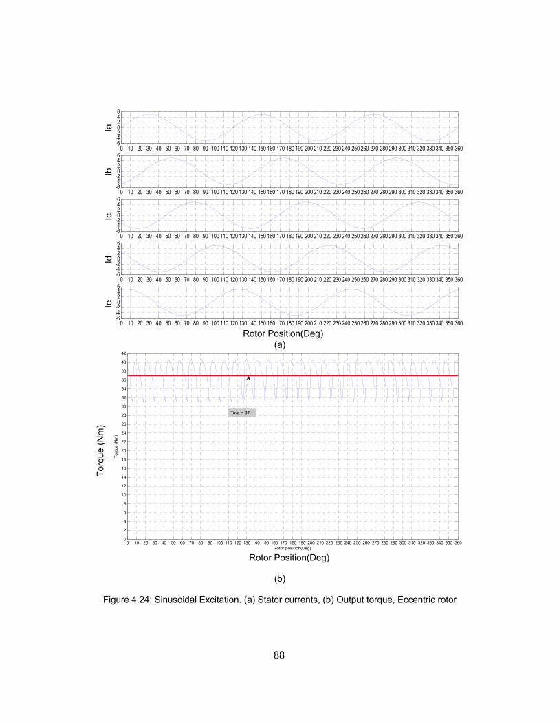
88

Ia

Ib

Ic

Id

Ie

Rotor Position(Deg) (a)

Tor

que

(Nm

)

Rotor Position(Deg)

(b)

Figure 4.24: Sinusoidal Excitation. (a) Stator currents, (b) Output torque, Eccentric rotor

0 10 20 30 40 50 60 70 80 90 100 110 120 130 140 150 160 170 180 190 200 210 220 230 240 250 260 270 280 290 300 310 320 330 340 350 360-6-4-20246

0 10 20 30 40 50 60 70 80 90 100 110 120 130 140 150 160 170 180 190 200 210 220 230 240 250 260 270 280 290 300 310 320 330 340 350 360-6-4-20246

0 10 20 30 40 50 60 70 80 90 100 110 120 130 140 150 160 170 180 190 200 210 220 230 240 250 260 270 280 290 300 310 320 330 340 350 360-6-4-20246

0 10 20 30 40 50 60 70 80 90 100 110 120 130 140 150 160 170 180 190 200 210 220 230 240 250 260 270 280 290 300 310 320 330 340 350 360-6-4-20246

0 10 20 30 40 50 60 70 80 90 100 110 120 130 140 150 160 170 180 190 200 210 220 230 240 250 260 270 280 290 300 310 320 330 340 350 360-6-4-20246

0 10 20 30 40 50 60 70 80 90 100 110 120 130 140 150 160 170 180 190 200 210 220 230 240 250 260 270 280 290 300 310 320 330 340 350 3600

2

4

6

8

10

12

14

16

18

20

22

24

26

28

30

32

34

36

38

40

42

Rotor position(Deg)

Tor

que

(Nm

)

Tavg = 37

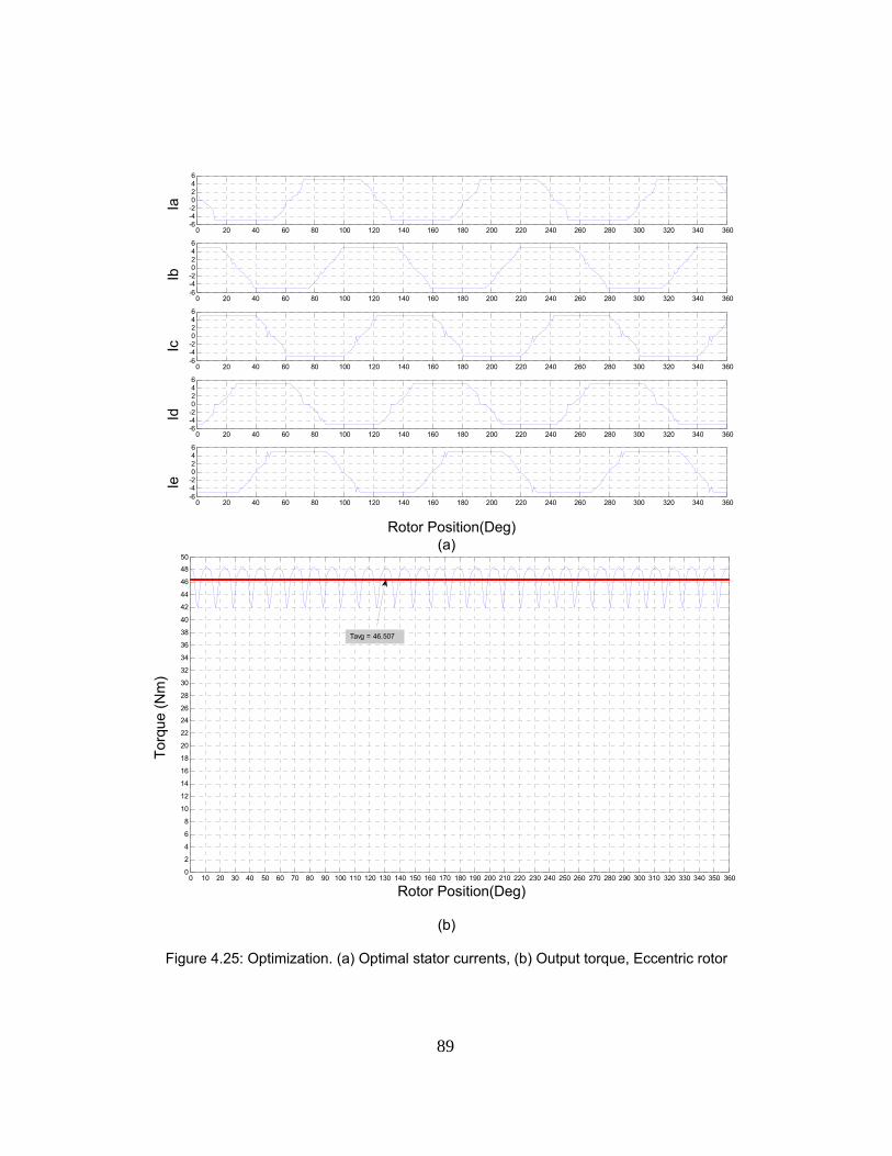
89

Ia

Ib

Ic

Id

Ie

Rotor Position(Deg) (a)

Tor

que

(Nm

)

Rotor Position(Deg)

(b)

Figure 4.25: Optimization. (a) Optimal stator currents, (b) Output torque, Eccentric rotor

0 20 40 60 80 100 120 140 160 180 200 220 240 260 280 300 320 340 360-6-4-20246

0 20 40 60 80 100 120 140 160 180 200 220 240 260 280 300 320 340 360-6-4-20246

0 20 40 60 80 100 120 140 160 180 200 220 240 260 280 300 320 340 360-6-4-20246

0 20 40 60 80 100 120 140 160 180 200 220 240 260 280 300 320 340 360-6-4-20246

0 20 40 60 80 100 120 140 160 180 200 220 240 260 280 300 320 340 360-6-4-20246

0 10 20 30 40 50 60 70 80 90 100 110 120 130 140 150 160 170 180 190 200 210 220 230 240 250 260 270 280 290 300 310 320 330 340 350 3600

2

4

6

8

10

12

14

16

18

20

22

24

26

28

30

32

34

36

38

40

42

44

46

48

50

Tavg = 46.507

90

Figure 4.25 depicts the output torque while the optimal currents have been applied to

stator phases. The optimization criteria are chosen so that the torque ripple would be minimized

and the average torque would be maximized.

4.5 Experimental Results

For independent control of phase currents which is required by fault tolerance, a full

bridge inverter has been used, which refers to the use of four switches connected in a bridge

arrangement as shown in figure 4.26. Control is performed by regulating the flow of current

through the stator windings of the machine. Current controllers are used to generate gate

signals for the inverter. Proper selection of the inverter devices and selection of the control

technique will guarantee the efficacy of the drive.

Figure 4.26: Current regulated full-bridge inverter used for the experimental 5-phase motor drive system

An electronically controlled PM motor drive system uses continuous rotor position

feedback and hystersis control to supply the motor with the appropriate current. The need of

knowing rotor position requires the development of devices for position measurement. In the

present drive system, the position sensor is mounted on the shaft of the rotor.

There are four devices that are commonly used for the measurement of position-

potentiometers, linear variable differential transformers, optical encoders and resolvers. Of

these, resolvers and encoders are most commonly used for motor drive applications.

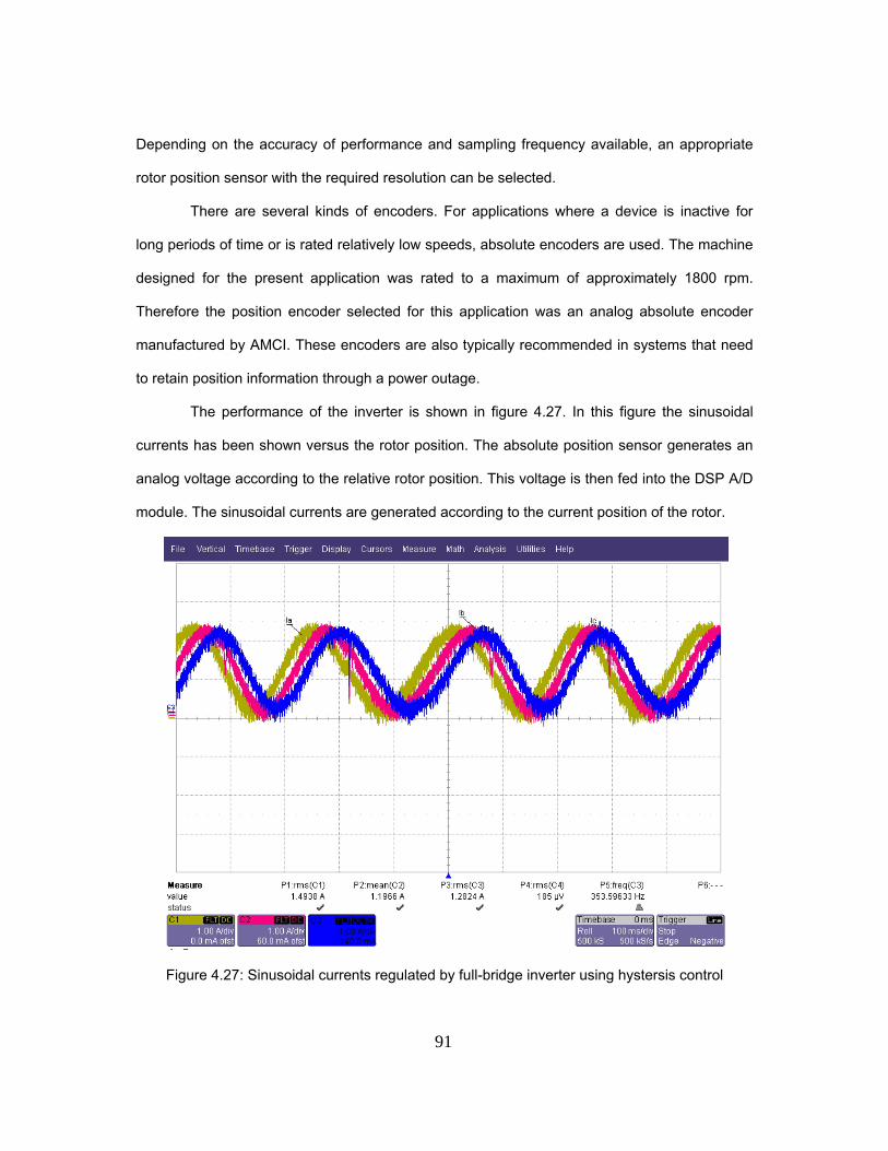
91

Depending on the accuracy of performance and sampling frequency available, an appropriate

rotor position sensor with the required resolution can be selected.

There are several kinds of encoders. For applications where a device is inactive for

long periods of time or is rated relatively low speeds, absolute encoders are used. The machine

designed for the present application was rated to a maximum of approximately 1800 rpm.

Therefore the position encoder selected for this application was an analog absolute encoder

manufactured by AMCI. These encoders are also typically recommended in systems that need

to retain position information through a power outage.

The performance of the inverter is shown in figure 4.27. In this figure the sinusoidal

currents has been shown versus the rotor position. The absolute position sensor generates an

analog voltage according to the relative rotor position. This voltage is then fed into the DSP A/D

module. The sinusoidal currents are generated according to the current position of the rotor.

Figure 4.27: Sinusoidal currents regulated by full-bridge inverter using hystersis control

92

Figure 4.28: Sinusoidal currents Applied to the motor

The sinusoidal excitation of the stator phases has been shown in figure 4.28. This figure

indicates the currents applied to phases “A” to “D”. In case one or more of the machine phases

undergo the open circuit fault, the DSP should be able to diagnose the fault location and apply

the appropriate currents to the remaining healthy phases. Figure 4.29 depicts the case in which

phase “B” of the machine is lost. The optimal currents have been calculated and stored using

Matlab optimization toolbox. These currents have been shown in figure 4.29(a). Figure 4.29(b)

depicts the actual currents obtained from the experimental test bed. The current waveform is

alos shown in figure 4.30 for a single phase.

Figure 4.31 depicts the optimal current applied to phase “A” of the motor. Figure 4.32

depicts the optimal currents in case of the double phase open circuit fault on the stator phases

“D” and “E”. The calculated optimal currents are shown in figure 4.32(a). The actual currents

applied to the stator healthy phases are shown in figure 4.32(b).

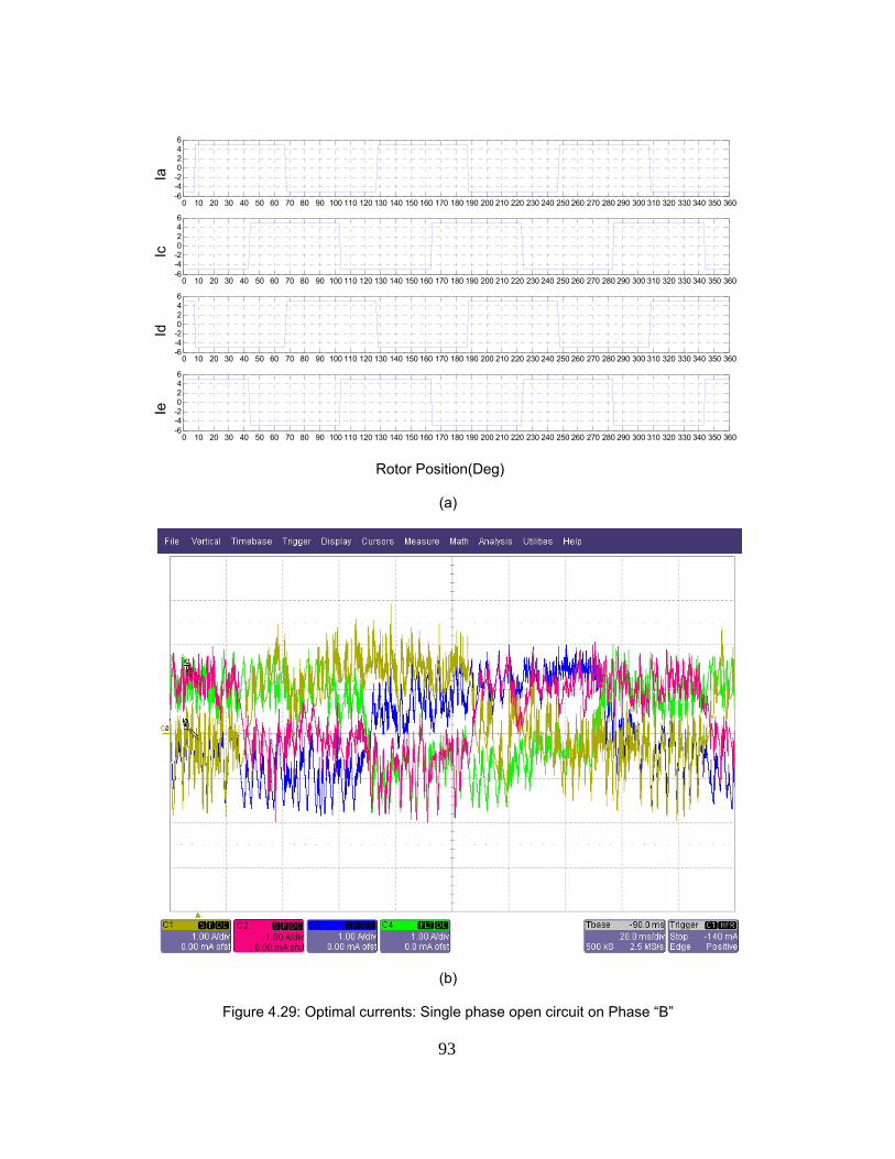
93

Ia

Ic

Id

Ie

Rotor Position(Deg)

(a)

(b)

Figure 4.29: Optimal currents: Single phase open circuit on Phase “B”

0 10 20 30 40 50 60 70 80 90 100 110 120 130 140 150 160 170 180 190 200 210 220 230 240 250 260 270 280 290 300 310 320 330 340 350 360-6-4-20246

0 10 20 30 40 50 60 70 80 90 100 110 120 130 140 150 160 170 180 190 200 210 220 230 240 250 260 270 280 290 300 310 320 330 340 350 360-6-4-20246

0 10 20 30 40 50 60 70 80 90 100 110 120 130 140 150 160 170 180 190 200 210 220 230 240 250 260 270 280 290 300 310 320 330 340 350 360-6-4-20246

0 10 20 30 40 50 60 70 80 90 100 110 120 130 140 150 160 170 180 190 200 210 220 230 240 250 260 270 280 290 300 310 320 330 340 350 360-6-4-20246

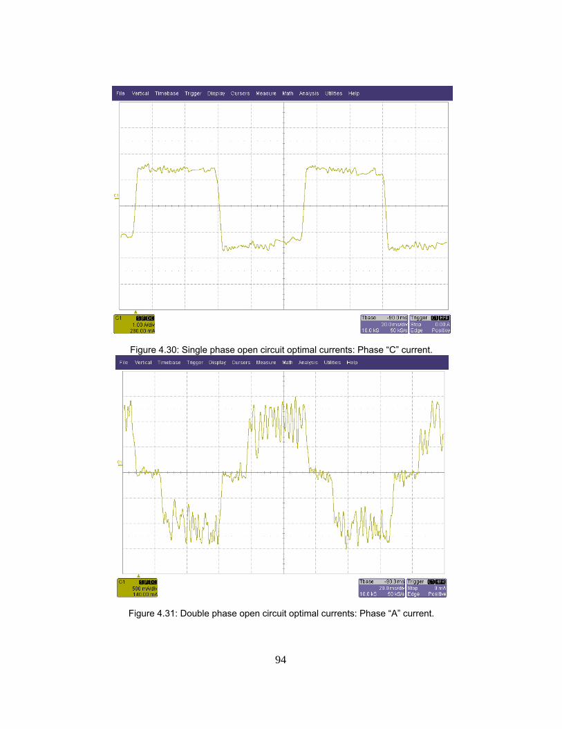
94

Figure 4.30: Single phase open circuit optimal currents: Phase “C” current.

Figure 4.31: Double phase open circuit optimal currents: Phase “A” current.

95

Ia

Ib

Ic

Rotor Position(Deg)

(a)

(b)

Figure 4.32: Optimal currents: Double phase open circuit on Phases “D” and “E”

0 10 20 30 40 50 60 70 80 90 100 110 120 130 140 150 160 170 180 190 200 210 220 230 240 250 260 270 280 290 300 310 320 330 340 350 360-6

-4

-2

0

2

4

6

0 10 20 30 40 50 60 70 80 90 100 110 120 130 140 150 160 170 180 190 200 210 220 230 240 250 260 270 280 290 300 310 320 330 340 350 360-6

-4

-2

0

2

4

6

0 10 20 30 40 50 60 70 80 90 100 110 120 130 140 150 160 170 180 190 200 210 220 230 240 250 260 270 280 290 300 310 320 330 340 350 360-6

-4

-2

0

2

4

6

96

Figure 4.33 compares the sinusoidal excitation of the stator phases compared with the

optimal case. The DC link voltage is 92(V). The rms value of the sinusoidal current is 0.7(A)

while the rms value of the optimal current is 0.63(A). The output torque of the machine in each

case has been shown in figure 4.34. According to this figure the output optimal torque is almost

%10 higher than the sinusoidal case. The significant achievement here is the reduction in the

torque ripple for optimal currents compared with sinusoidal excitation.

(a)

(b)

Figure 4.33: Torque Analysis. (a) Sinusoidal current, (b) Optimal current.

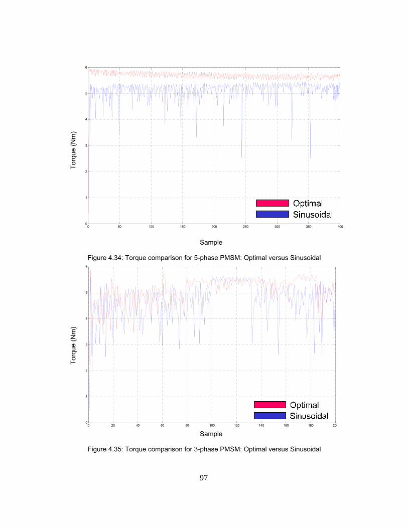
97

Tor

que

(Nm

)

0 50 100 150 200 250 300 350 4000

1

2

3

4

5

6

Sample

Figure 4.34: Torque comparison for 5-phase PMSM: Optimal versus Sinusoidal

Tor

que

(Nm

)

0 20 40 60 80 100 120 140 160 180 2000

1

2

3

4

5

6

Sample

Figure 4.35: Torque comparison for 3-phase PMSM: Optimal versus Sinusoidal

98

T

orqu

e (N

m)

0 20 40 60 80 100 120 140 160 180 2000

1

2

3

4

5

6

7

SinusoidalOptimal

Sample

Figure 4.36: Torque comparison for 4-phase PMSM: Optimal versus Sinusoidal

Figures 4.35 and 4.36 depict the torque comparison for the double and single phase

open-circuit faults. According to the figures, the average torque is higher in case of optimal

excitation compared with the sinusoidal operation of the machine. The torque per ampere is

better in case of 5–phase and 3-phase operation while in case of 4-phase operation sinusoidal

excitation gets better results. In terms of ripple the optimal excitation is significantly better

compared with the sinusoidal case.

99

CHAPTER 5

CONCLUSIONS

Fault tolerance operation of the adjustable motor drives is crucial in high impact

applications. Fault detection and optimal post fault treatment of the fault are the basic

requirements for the operation.

In this dissertation, a field reconstruction method based on Finite Element Analysis has

been developed. This method involves the reconstruction of the electromagnetic fields due to

the phase currents using basis functions obtained using one single solution from FEA. The field

reconstruction method presents a new numerical technique for analysis and design of a PMSM.

This technique is time- efficient and offers an insightful vision of the magnetic field in the

machine. It combines ideas from electromechanical energy conversion, signal reconstruction,

pattern recognition, and power electronics to create novel solutions. By manipulating the

tangential and normal components of magnetic field in the airgap of the machine, the magnetic

flux passing through each stator tooth can be estimated. These fluxes are used to estimate the

flux linking each stator phase. The flux estimated is used to detect the signatures related to

each of open circuit, partial demagnetization and rotor eccentricity faults. The fault treatment

has been investigated by comparing the optimal and sinusoidal excitation of the stator phases.

It is shoen that in case of optimal currents the average torque is higher compared with the

sinusoidal and the ripple is smaller.

100

APPENDIX A

EXPERIMENTAL TESTBED SETUP

101

Experimental test bed including the 5-phase PMSM, Torque meter, Dynamometer and Power Electronics boards

5-phase PMSM coupled to the absolute position encoder

102

APPENDIX B

ROTOR AND STATOR LAMINATION

103

5-phase PMSM stator and rotor laminations

104

APPENDIX C

COIL WINDINGS ARRANGEMENT

105

PMSM 6-pole, 5-phase, 30-slot stator and 6-pole rotor

106

APPENDIX D

POWER ELECTRONICS CONVERTER

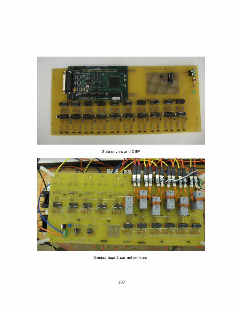
107

Gate drivers and DSP

Sensor board: current sensors

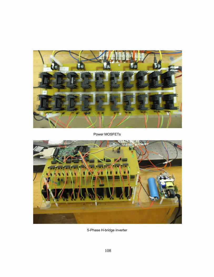
108

Power MOSFETs

5-Phase H-bridge inverter

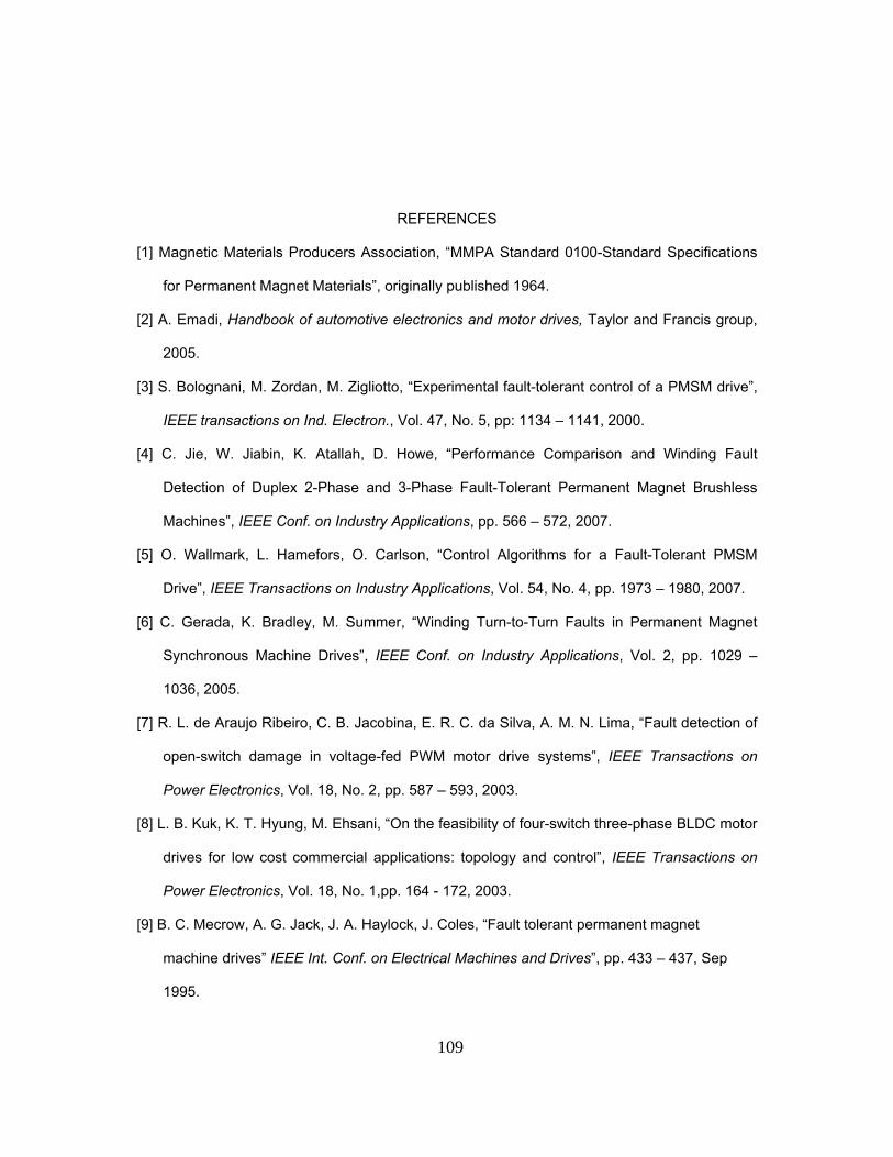
109

REFERENCES

[1] Magnetic Materials Producers Association, “MMPA Standard 0100-Standard Specifications

for Permanent Magnet Materials”, originally published 1964.

[2] A. Emadi, Handbook of automotive electronics and motor drives, Taylor and Francis group,

2005.

[3] S. Bolognani, M. Zordan, M. Zigliotto, “Experimental fault-tolerant control of a PMSM drive”,

IEEE transactions on Ind. Electron., Vol. 47, No. 5, pp: 1134 – 1141, 2000.

[4] C. Jie, W. Jiabin, K. Atallah, D. Howe, “Performance Comparison and Winding Fault

Detection of Duplex 2-Phase and 3-Phase Fault-Tolerant Permanent Magnet Brushless

Machines”, IEEE Conf. on Industry Applications, pp. 566 – 572, 2007.

[5] O. Wallmark, L. Hamefors, O. Carlson, “Control Algorithms for a Fault-Tolerant PMSM

Drive”, IEEE Transactions on Industry Applications, Vol. 54, No. 4, pp. 1973 – 1980, 2007.

[6] C. Gerada, K. Bradley, M. Summer, “Winding Turn-to-Turn Faults in Permanent Magnet

Synchronous Machine Drives”, IEEE Conf. on Industry Applications, Vol. 2, pp. 1029 –

1036, 2005.

[7] R. L. de Araujo Ribeiro, C. B. Jacobina, E. R. C. da Silva, A. M. N. Lima, “Fault detection of

open-switch damage in voltage-fed PWM motor drive systems”, IEEE Transactions on

Power Electronics, Vol. 18, No. 2, pp. 587 – 593, 2003.

[8] L. B. Kuk, K. T. Hyung, M. Ehsani, “On the feasibility of four-switch three-phase BLDC motor

drives for low cost commercial applications: topology and control”, IEEE Transactions on

Power Electronics, Vol. 18, No. 1,pp. 164 - 172, 2003.

[9] B. C. Mecrow, A. G. Jack, J. A. Haylock, J. Coles, “Fault tolerant permanent magnet

machine drives” IEEE Int. Conf. on Electrical Machines and Drives”, pp. 433 – 437, Sep

1995.

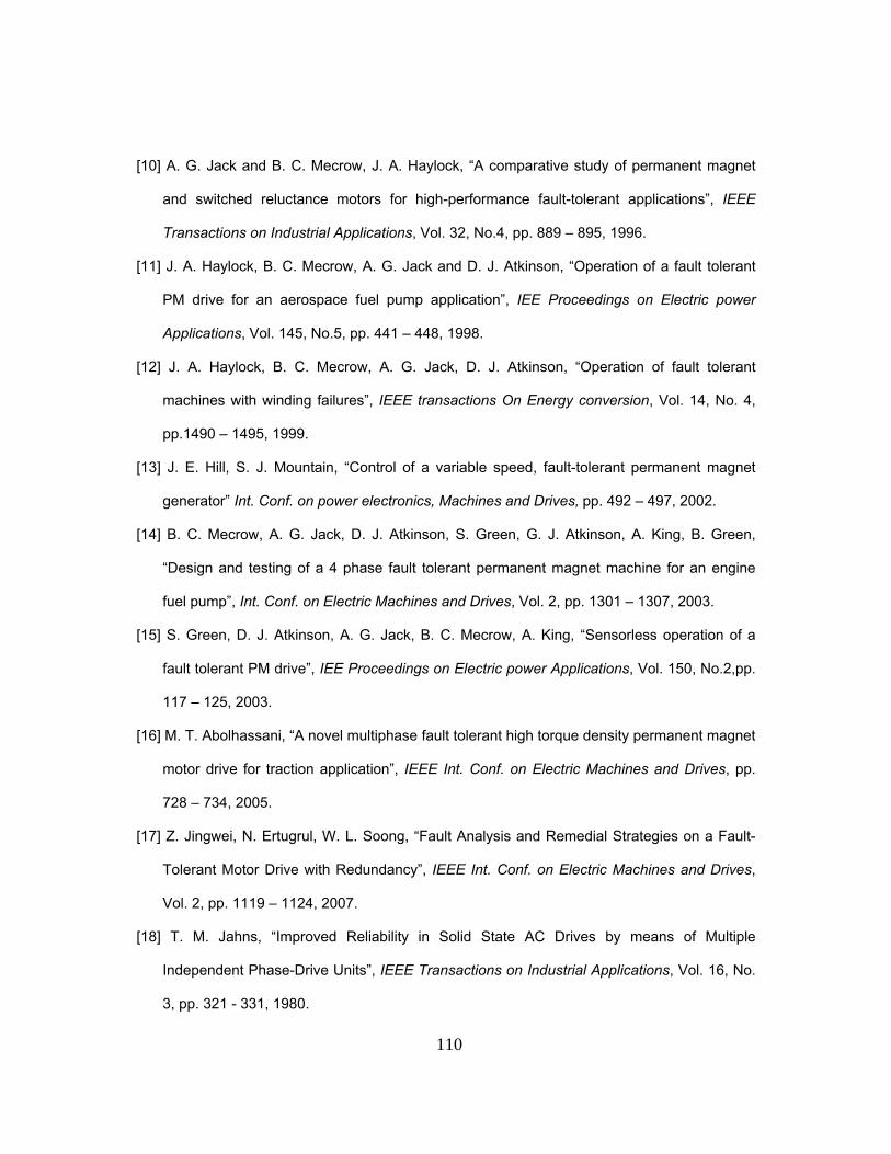
110

[10] A. G. Jack and B. C. Mecrow, J. A. Haylock, “A comparative study of permanent magnet

and switched reluctance motors for high-performance fault-tolerant applications”, IEEE

Transactions on Industrial Applications, Vol. 32, No.4, pp. 889 – 895, 1996.

[11] J. A. Haylock, B. C. Mecrow, A. G. Jack and D. J. Atkinson, “Operation of a fault tolerant

PM drive for an aerospace fuel pump application”, IEE Proceedings on Electric power

Applications, Vol. 145, No.5, pp. 441 – 448, 1998.

[12] J. A. Haylock, B. C. Mecrow, A. G. Jack, D. J. Atkinson, “Operation of fault tolerant

machines with winding failures”, IEEE transactions On Energy conversion, Vol. 14, No. 4,

pp.1490 – 1495, 1999.

[13] J. E. Hill, S. J. Mountain, “Control of a variable speed, fault-tolerant permanent magnet

generator” Int. Conf. on power electronics, Machines and Drives, pp. 492 – 497, 2002.

[14] B. C. Mecrow, A. G. Jack, D. J. Atkinson, S. Green, G. J. Atkinson, A. King, B. Green,

“Design and testing of a 4 phase fault tolerant permanent magnet machine for an engine

fuel pump”, Int. Conf. on Electric Machines and Drives, Vol. 2, pp. 1301 – 1307, 2003.

[15] S. Green, D. J. Atkinson, A. G. Jack, B. C. Mecrow, A. King, “Sensorless operation of a

fault tolerant PM drive”, IEE Proceedings on Electric power Applications, Vol. 150, No.2,pp.

117 – 125, 2003.

[16] M. T. Abolhassani, “A novel multiphase fault tolerant high torque density permanent magnet

motor drive for traction application”, IEEE Int. Conf. on Electric Machines and Drives, pp.

728 – 734, 2005.

[17] Z. Jingwei, N. Ertugrul, W. L. Soong, “Fault Analysis and Remedial Strategies on a Fault-

Tolerant Motor Drive with Redundancy”, IEEE Int. Conf. on Electric Machines and Drives,

Vol. 2, pp. 1119 – 1124, 2007.

[18] T. M. Jahns, “Improved Reliability in Solid State AC Drives by means of Multiple

Independent Phase-Drive Units”, IEEE Transactions on Industrial Applications, Vol. 16, No.

3, pp. 321 - 331, 1980.

111

[19] A. G. Jack and B. C. Mecrow, “Safety Critical Drives for Aerospace Applications”,

Proceedings of ICEM 94, Vol. 1, pp.91-96, 1994.

[20] R. V. White, “Fault tolerance in distributed power systems”, Proceedings of EPE’95, pp. 2

851-2 857, 1995.

[21] J. Zhu, N. Ertugrul, W. L. Soong, “Performance Investigation of a Fault-Tolerant Brushless

Permanent Magnet AC Motor Drive” IEEE Int. Conf. on Power Electronics and Motion

Control, Vol. 2, pp. 1 – 5, 2006.

[22] Z. Jingwei, N. Ertugrul, W. L. Soong, “Detection and Remediation of Switch Faults on a

Fault Tolerant Permanent Magnet Motor Drive with Redundancy”, IEEE Conf. on Industrial

Electronics and Applications, pp. 96 – 101, 2007.

[23] J. Penman, H. G. Sedding, B. A. Lloyd, W.T. Fink, “Detection and Location of Inter turn

Short Circuits in the Stator Windings of Operating Motors”, IEEE Transactions on Energy

Conversion, Vol. 9, No. 4, pp. 652-658, Dec. 1994.

[24] E. Wosdmagg “Turbo generator Field Winding Shorted Turn Detection by AC Flux

Measurement”, IEEE Transactions on Energy Conversion, Vol. 9, No. 2, pp. 427.431, June

1994.

[25] K. Weinreh, P. Drozdavski, “Detection of Winding Faults of a Salient Pole Synchronous

Modeling by a Spectral Analysis of Currents”, ICEM 94, Vol. 2, pp. 56-61, 1994.

[26] W. Jiabin, K. Atallah, D. Howe, “Optimal torque control of fault-tolerant permanent magnet

brushless machines”, IEEE transactions on Magnetics, Vol. 39, No. 5, pp. 2962 – 2964,

2003.

[27] W. Zhu, B. Fahimi, S. Pekarek, “A field reconstruction method for optimal excitation of

permanent magnet synchronous machines”, IEEE Trans. on Energy Conversion, vol. 21,

no.2, pp. 305 – 313, June 2006.

112

[28] B. Fahimi, “Qualitative approach to electromechanical energy conversion: Reinventing the

art of design in adjustable speed drives”, ICEMS Int. Conf. on Electrical machines and

Systems, pp. 432 – 439, Oct 2007.

[29] W. Jiang, M. Moallem, B. Fahimi, S. Pekarek, “Qualitative Investigation of Force Density

Components in Electromechanical Energy Conversion Process”, IEEE Conf. on Ind.

Electron., pp.1113-1118, Nov. 2006.

[30] W. Zhu, B. Fahimi, S. Pekarek, “Optimal excitation of permanent magnet synchronous

machines via direct computation of electromagnetic force components”, IEEE Int. Conf. on

Electrical machines and Drives, pp. 918 - 925 , May 2005.

[31] P. C. Krause, Analysis of Electric Machinery, McGraw- Hill, 1986, New York.

[32] J. Holtz, “Methods for speed sensorless control of AC drives,” in Sensorless Control of AC

Motor Drives, K. Rajashekara, A. Kawamura, and K. Matsuse, Eds. Piscataway, NJ: IEEE

Press, 1996.

[33] J. Jinsheng, J. Holtz, “High dynamic speed sensorless AC drive with on-line model

parameter tuning for steady state accuracy”, IEEE Trans. on Ind. Electron., vol. 44, no.2,

pp. 240 – 246, Apr 1997.

[34] J. Holtz, Q. Juntao, “Sensorless vector control of induction motors at very low speed using a

nonlinear inverter model and parameter identification”, IEEE Trans. on Ind. Appicatl., vol.

38, no.4, pp. 1087 – 1095, July 2002.

[35] J. Holtz, “Acquisition of position error and magnet polarity for sensorless control of PM

synchronous machines”, IEEE Trans. on Ind. Appicatl., vol. 44, no.4, pp. 1172 – 1180, July

2008.

[36] J. Holtz, “Sensorless position control of induction motors - an emerging technology”, IEEE

Trans. on Ind. Electron., vol. 45, no.6, pp. 840 – 851, Dec 1998.

[37] P. L. Jansen and R. D. Lorenz, “Transducerless position and velocity estimation in induction

and salient AC machines,” IEEE Trans. Ind. Applicat., vol. 31, pp. 240–247, Mar./Apr 1995.

113

[38] Y. A. Chapuis. D. Roye, J. Davoine, “Principles and implementation of direct torque control

by stator flux orientation of an induction motor”, IEEE IAS annual meeting, vol. 1, pp. 185 –

191, 1995.

[39] B. K. B. And, N. R. Patel, “A programmable cascaded low-pass filter based flux synthesis

for a stator flux-oriented vector-controlled induction motor drive”, IEEE Trans. on Ind.

Electron., vol. 44, no.1, pp. 140 – 143, Feb 1997.

[40] M. F. Rahman, M. E. Haque, L. Tang, L. Zhong, “Problems associated with the direct torque

control of an interior permanent magnet synchronous motor drive and their remedies ”,

IEEE Trans. on Ind. Electron., vol. 51, no. 4, pp. 799 - 809, Aug 2004.

[41] K. K. Shyu, L. J. Shang, H. Z. Chen, K. W. Jwo, “Flux compensated direct torque control of

induction motor drives for low speed operation”, IEEE Trans. on Power Electron., vol. 19,

no. 6, pp. 1608 - 1613, Nov. 2004.

[42] S. Mir, M. E. Elbuluk, D. S. Zinger, “PI and fuzzy estimators for tuning the stator resistance

in direct torque control of induction machines”, IEEE Trans. on Power Electron. vol. 13, no.

2, pp. 279 – 287, Mar 1998.

[43] L. Zhong, M. F. Rahman, K. W. Lim, Y. Hu, Y. Xu, “A fuzzy observer for induction motor

stator resistance for applications in direct torque control”, IEEE Int. Conf. on Power

Electronics and drive systems , pp. 91 - 96, 1997.

[44] F. Zidani, D, Diallo, M. E. H. Benbouzid, R. Nait-Said, “Direct torque control of induction

motor with fuzzy stator resistance adaption”, IEEE Trans on Energy Conversion, Vol. 21,

no. 2, pp. 619 - 621, June 2006.

[45] E. Wosdmagg, “Turbo generator Field Winding Shorted Turn Detection by AC Flux

Measurement”, IEEE Trans on Energy Conversion, Vol. 9, no. 2, pp. 427 - 431, June 1994.

[46] C. C. Wang, C. H. Fang, “Sensorless scalar controlled induction motor drives with modified

flux observer”, IEEE Trans. on Energy Conversion, vol. 18, no.2, pp. 181 – 186, June 2003.

114

[47] V. Vasic, S. N. Vukosavic, E. Levi, “A stator resistance estimation scheme for speed

sensorless rotor flux oriented induction motor drives”, IEEE Trans. on Energy Conversion,

vol. 18, no.4, pp. 476 – 483, Dec 2003.

[48] S. B. Lee, T. G. Habetler, R. G. Harley, D. J. Gritter, “An evaluation of model-based stator

resistance estimation for induction motor stator winding temperature monitoring”, IEEE

Trans. on Energy Conversion, vol. 17, no.1, pp. 7 – 15, Mar 2002.

[49] H. D. Glass, B. C. Brown, G. W. Foster, W. B. Fowler, R. Gustafson, G. P. Jackson, J. F.

Ostiguy, J. T. Volk, “Stability tests of permanent magnets built with strontium ferrite”,

Particle Accelerator Conference, Vol. 3, pp. 3260 – 3262, May 1997.

[50] S. Ruoho, A. Arkkio, “Partial Demagnetization of Permanent Magnets in Electrical

Machines Caused by an Inclined Field”, IEEE Trans. on Magnetics, Vol. 44, pp. 1773 –

1778, July 2008.

[51] J. R. Riba Ruiz, J. A. Rosero, A. Garcia Espinosa, L. Romeral, “Detection of

Demagnetization Faults in Permanent-Magnet Synchronous Motors Under Nonstationary

Conditions”, IEEE Trans. on Magnetics, vol. 45, No. 7, pp. 2961 – 2969, 2009

[52] J. Rosero, L. Romeral, J. A. Ortega, J.C. Urresty, “Demagnetization fault detection by

means of Hilbert Huang transform of the stator current decomposition in PMSM”, Int. Sym.

on Industrial Electronics (ISIE), pp. 172 – 177, 2008

[53] J. A. Rosero, J. Cusido, A. Garcia, J. A. Ortega, L. Romeral, “Study on the Permanent

Magnet Demagnetization Fault in Permanent Magnet Synchronous Machines”, IEEE conf.

on Industrial Electronics, pp. 879 – 884, 2006.

[54] B. M. Ebrahimi, J. Faiz, M.J. Roshtkhari, “ Static-, Dynamic-, and Mixed-Eccentricity fault

diagnoses in permanent-magnet synchronous motors”, IEEE Trans. on Ind. Electron., Vol.

56, No. 11, pp. 4727– 4739, 2009.

115

BIOGRAPHICAL INFORMATION

Amir Khoobroo was born on November 19, 1979 in Tehran, Iran. He received his

Bachelor of Science from Sharif University of technology, Tehran, Iran, in 2003 and Master of

Science in Electrical Machines and Drives from the Isfahan University of techology, Isfahan,

Iran, in 2006. He started his PhD in Spring 2007 at the University of Texas at Arlington.During

his PhD, he was employed at Renewable Energy and Vehicular technology Laboratory as a

Research Associate where he was involved in the design and implementation of Electrical

machines and Power Electronics modules. At the University of Texas at Arlington, he was also

involved in various projects including the design of linear Switched Reluctance machines and

development of the power electronics drilling applications. His research interests include power

electronics, motor drives, renewable energy and vehicular systems.