Fátima Sánchez Cabo - Bioinformatics...

07/03/2007 - p. 1/35

Introduction to probability theory

Fátima Sánchez CaboInstitute for Genomics and Bioinformatics, TUGraz

[email protected]

Probability Theory: Random

experiments

Conditional probability

Random variables and their

distributions

References

07/03/2007 - p. 2/35

Outline

Random experiments and conditional probability (7 March)

Random variables and their distributions

From Probability Theory to Statistics (14 March)

Hypothesis testing (14 March)

Stochastic processes and Markov chains (21 March)


experiments

Introduction

Definition

Sample space and events

Probability Space

Algebra of Sets

Probability measure

Example



distributions

References

07/03/2007 - p. 3/35

Probability Theory: Random experiments


experiments

Introduction

Definition


Probability Space

Algebra of Sets

Probability measure

Example



distributions

References

07/03/2007 - p. 4/35

Introduction

Life is full of unpredictable events

Probabilistic models are used to make inference from thistype of experiments: their outcome cannot be completelydetermined, but we can get some hints about the mostlikely situation that will occur

Randomness does not mean chaos: for example themost likely value in a normally distributed random variableis the mode; very small or very large values are veryunlikely to occur

−4 −3 −2 −1 0 1 2 3 40

0.05

0.1

0.15

0.2

0.25

0.3

0.35

0.4

Normal(0,1)


experiments

Introduction

Definition


Probability Space

Algebra of Sets

Probability measure

Example



distributions

References

07/03/2007 - p. 5/35

Random experiments: Definition

All outcomes of the experiment are known in advance

But, it is a priori unknown which will be the outcome ofeach performance of the experiment:

Systematic and random errorsComplex processes, result of many combined processes

The experiment can be repeated under identical conditions


experiments

Introduction

Definition


Probability Space

Algebra of Sets

Probability measure

Example



distributions

References

07/03/2007 - p. 6/35

Examples

Throwing a die:Possible outcomes: 1,2,3,4,5,6It is unknown what we will get next if we throw the dieWe can throw the die n times and all are independenttrials

Tossing a coin:Possible outcomes: head, tailIt is unknown what we will get next if we toss the coinWe can toss the coin n independent times

The length life of a light bulb produced by a manufacturer:Possible outcomes: Any number between 0 and ∞The life-time of a bulb is not known before handWe assume that the life-time of n bulbs can be measuredunder the same conditions


experiments

Introduction

Definition


Probability Space

Algebra of Sets

Probability measure

Example



distributions

References

07/03/2007 - p. 7/35

Sample space, events, σ algebra

Sample space: Collection of possible elementary outcomesfrom a random experiment.1. Throwing a die: Ω=1,2,3,4,5,62. Tossing a coin: Ω=head, tail3. Life-time of a bulb: Ω = [0,∞)

Event: A set of outcomes of the experiment.1. Throwing a die: "To obtain a 6" (6) or "Not to obtain a

6" (1,2,3,4,5)2. Tossing a coin: "To obtain a head"

3. Life-time of a bulb: "The life-time of the bulb is greaterthan 3 years"

A σ-field (or σ-algebra) is a non-empty collection of subsetsof Ω that satisfy:

∅ ǫ Fif A ǫ F then Ac ǫ F ,andif Ai ǫ F is a countable sequence of sets then

⋃

i Ai ǫ F


experiments

Introduction

Definition


Probability Space

Algebra of Sets

Probability measure

Example



distributions

References

07/03/2007 - p. 8/35

Probability space

The pair (Ω,F) is called under the previous conditions asample space

A measure is a nonnegative countably additive setfunction , i.e. a function µ : F → R such as:1. µ(A) ≥ µ(∅) for all AǫF , and2. if Ai ǫ F and

⋂

i Ai = ∅ then µ(⋃

i Ai) =∑

i µ(Ai)a

If µ(Ω) = 1 the measure is called a probability measureacountable: the set of the natural number, uncountable: the set of the real numbers


experiments

Introduction

Definition


Probability Space

Algebra of Sets

Probability measure

Example



distributions

References

07/03/2007 - p. 9/35

A little on Algebra of Sets

Sets algebra is equivalent to elementary algebra(arithmetic): Intersection → Multiplication; Union →Addition

Differently from arithmetic operations (only distributive forthe product) union and intersection have both thedistributive property

Uniqueness of complements:Given A, B such as A ∪B = Ω and A ∩B = ∅, then B = Ac

B\A = B ∩ Ac

Morgan’s Laws:(A ∪ B)c = Ac ∩ Bc

(A ∩ B)c = Ac ∪ Bc

Acc = A

∅c = Ω; Ωc = ∅


experiments

Introduction

Definition


Probability Space

Algebra of Sets

Probability measure

Example



distributions

References

07/03/2007 - p. 10/35

Probability measure

Some properties of the probability measure:1. P (A ∪ B) = P (A) + P (B) − P (A ∩ B)

2. P (Ac) = 1 − P (A)

3. If B ⊇ A ⇒ P (B) = P (A) + P (B\A) ≥ P (A)

4. In general, if A1, . . . , AnǫF ⇒

P (⋃

Ai) =

=∑

P (Ai) −∑

i<j

P (Ai ∩ Aj) − . . . + (−1)n+1P (A1 ∩ . . . ∩ An)

Exercise: Proof 1-3


experiments

Introduction

Definition


Probability Space

Algebra of Sets

Probability measure

Example



distributions

References

07/03/2007 - p. 11/35

Example

The probability of a chicken from Steiermark to be infected withthe Bird flu is 0.2 a. At the same time a chicken may haveanother lethal disease called Y that appears with probability0.5. Calculate the probability of chicken dying due to anydisease:1. If it is not possible that both diseases appear

simultaneously;2. If the probability of having both diseases is 0.6.

aUnreal number


experiments


Dependent events

Definition

Example

Bayes’ Theorem


distributions

References

07/03/2007 - p. 12/35



experiments


Dependent events

Definition

Example

Bayes’ Theorem


distributions

References

07/03/2007 - p. 13/35

Dependent events

P(B )=2/3 P(W )=1/3

P(B )=1/3 P(W )=2/3

Which is the probability of getting a white ball? Is the same inboth experiments?


experiments


Dependent events

Definition

Example

Bayes’ Theorem


distributions

References

07/03/2007 - p. 14/35

Dependent events

Definition:Two events A, B are called independent ifP (A ∩ B) = P (A) · P (B). Otherwise,P (A ∩ B) = P (A) · P (B |A) = P (B) · P (A |B)

Multiplication rule:Given a probability space (Ω,F ,P) such as A1, . . . , AnǫF

and P (∩n−1i=1 Ai) > 0, then

P (∩ni=1Ai) = P (A1)P (A2 |A1) . . . P (An | ∩n−1

i=1 Ai)


experiments


Dependent events

Definition

Example

Bayes’ Theorem


distributions

References

07/03/2007 - p. 15/35


Definition:(Ω,F ,P) is a probability space such as the events A and B

ǫ F . If P (B) > 0 it can be defined the probability of A

conditional on B as:

P (A |B) =P (A ∩ B)

P (B)

Total probability theorem:Let Ω be the sample space of a random experiment andAi, i = 1, 2, . . . ǫ F such as Ai

⋂

Aj = ∅ ∀i 6= j and⋃

i Ai = Ω. Then, for all B ǫ F

P (B) =∑

i

P (B |Ai)P (Ai)


experiments


Dependent events

Definition

Example

Bayes’ Theorem


distributions

References

07/03/2007 - p. 16/35

Example

The probability of a chicken from Steiermark to be infected withthe Bird flu is 0.2 a. At the same time a chicken may haveanother lethal disease called Y that appears with probability0.5. The death rate if a chicken has the Bird Flu is 0.8. Theprobability of death for a chicken with disease Y is 0.1. Bothdiseases cannot appear simultaneously. Additionally, a chickenmight die due to natural causes with a probability 0.1.Calculate the probability of dying for a chicken in Steiermark.

aUnreal number


experiments


Dependent events

Definition

Example

Bayes’ Theorem


distributions

References

07/03/2007 - p. 17/35

Bayes’ Theorem

Let Ω be the sample space of a random experiment andAi, i = 1, 2, . . . ǫ F such as Ai

⋂

Aj = ∅ ∀i 6= j and⋃

i Ai = Ω. Let B ǫ F with P(B)>0. Then

P (Ai |B) =P (B ∩ Ai)

P (B)

Equivalently,

P (Ai |B) =P (B |Ai)P (Ai)

∑

j P (B |Aj)P (Aj)


experiments


Dependent events

Definition

Example

Bayes’ Theorem


distributions

References

07/03/2007 - p. 18/35

Example

3

2

1

Door C Door B Door A

3

2

1



experiments


Dependent events

Definition

Example

Bayes’ Theorem


distributions

References

07/03/2007 - p. 19/35

Example

3

2

1


3

2

1


Naive approach: Regardless to the initial situation nowthere are only two doors from which I could choose. Hence,Pr(car is behind A)=Pr(car is not behind A)= 1

2

It is not an advantage to switch the door.

By Bayes’ Theorem: ⇒


experiments


Dependent events

Definition

Example

Bayes’ Theorem


distributions

References

07/03/2007 - p. 20/35

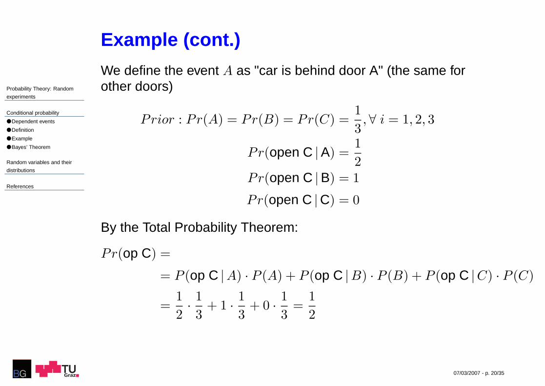
Example (cont.)

We define the event A as "car is behind door A" (the same forother doors)

Prior : Pr(A) = Pr(B) = Pr(C) =1

3, ∀ i = 1, 2, 3

Pr(open C |A) =1

2Pr(open C |B) = 1

Pr(open C |C) = 0

By the Total Probability Theorem:

Pr(op C) =

= P (op C |A) · P (A) + P (op C |B) · P (B) + P (op C |C) · P (C)

=1

2·1

3+ 1 ·

1

3+ 0 ·

1

3=

1

2


experiments


Dependent events

Definition

Example

Bayes’ Theorem


distributions

References

07/03/2007 - p. 21/35

Example (cont.)

By Bayes’ Theorem:

Pr(A |open C) =Pr(open C |A) · Pr(A)

Pr(open C)=

12 · 1

312

=1

3

Pr(B |open C) =Pr(open C |B) · Pr(B)

Pr(open C)=

1 · 13

12

=2

3

Conclusion: The probability of winning the car is bigger if youchange the door!!!


experiments



distributions

Random variable

Continuous random variables

Distribution function

Expectation and variance

Central Limit Theorem

References

07/03/2007 - p. 22/35

Random variables and their distributions


experiments



distributions

Random variable





References

07/03/2007 - p. 23/35

Random variable

The probability measure P is a set function and hencedifficult to work with it.

We define a random variable on a probability space as areal valued function X defined in Ω such as:

X : Ω → R and X−1(B) = ω : X(ω)ǫBǫF , for all Borel set B ⊂ R

In other words, if the inverse of any Borel subset of R

(semi-open intervals) belongs to the σ-algebra

Example: The random experiment "To toss a coin" can berepresented with the random variable

X =

1 if Head(⇒ X−1(1) = HeadǫF)

0 if Tail(⇒ X−1(0) = TailǫF)


experiments



distributions

Random variable





References

07/03/2007 - p. 24/35

Example 3.1.

A roulette wheel has 38 slots -18 red, 18 black and 2 green.A gambler bets 1 $ to red each time. We define the randomvariable Xi as the monetary gain of the gambler at game i.(From Durret (1996))

Ω = Red, Black, Green

Events:F =Red, Black, Green, Red, Black, Red, Green, Black, Green,Red, Black, Green, ∅

P (Red) = 1838 = 9

19 ,P (no Red) = 20

38 = 1019

Random variable:

X =

+1 Red−1 ¬Red


experiments



distributions

Random variable





References

07/03/2007 - p. 25/35

Discrete random variables

A discrete random variable can take a countable number ofpredetermined values

Example: "To toss a coin", "To throw a die", "Number ofcars crossing a line during a certain time interval"

Mass function: For discrete random variables, the massfunction determines the probability of each element of thesample space.

Example: for the random experiment "To throw a die"p(1) = . . . = p(6) = 1

6

1 2 3 4 5 6 7 8 90

5

10

15

20

25

Mass probability function of 100 random numbers from a binomial distribution (n=100, p=0.5)


experiments



distributions

Random variable





References

07/03/2007 - p. 26/35

Discrete random variables

Typical mass functions of discrete random variables:

1. Bernoulli :

X =

1 p

0 (1 − p)

2. Binomial: Number of successes within n Bernoulli trials:

P (X = k) = C(n, k)pk(1 − p)n−k

3. Poisson , P (X = k) = e−λλk

k!


experiments



distributions

Random variable





References

07/03/2007 - p. 27/35


For continuous random variables (that can take any real value)the way the probability is distributed within the sample space ismore difficult to define. The probability density function(pdf) has the following properties:

1. P [a ≤ X ≤ b] =∫ b

af(x)dx

2. f(x) ≥ 0, ∀xǫR

3.∫ ∞

−∞f(x)dx = 1

−4 −3 −2 −1 0 1 2 3 40

20

40

60

80

100

120

140

160

180

200

Histogram of frequencies for a normal random variable


experiments



distributions

Random variable





References

07/03/2007 - p. 28/35


Most usual pdf

1. Normal distributionf(x) = 1√

2πσ2· exp− (x−µ)2

2σ2

Random errors are normally distributed

2. Uniform f(x) = 1b−a

· I[a,b]

3. Gamma f(x) = βα

Γ(α)xα−1e−βx


experiments



distributions

Random variable





References

07/03/2007 - p. 29/35


F (x) = P (X ≤ x) =

∫ x

af(x)dx cont r.v.

∑xa P (X = k) discrete r.v.

where a is the smallest value that the r.v. can take.

1 2 3 4 5 6 7 8 90

0.1

0.2

0.3

0.4

0.5

0.6

0.7

0.8

0.9

1

x

F(x

)

Empirical CDF

−4 −3 −2 −1 0 1 2 3 40

0.1

0.2

0.3

0.4

0.5

0.6

0.7

0.8

0.9

1

x

F(x

)

Empirical CDF

Probability distribution of 100 random numbers from a binomial distribution (n=10, p=0.5) and cumulative probability

distribution of 1000 random numbers from a normal distribution (µ=0, σ2=1)


experiments



distributions

Random variable





References

07/03/2007 - p. 30/35

Example 3.2.

A fair coin (p=0.5) is tossed twice. For each one of the possibleoutcomes of the experiment we define the random variable thatindicates the number of heads, i.e.:

X =

2 HH1 HT,TH0 TT

Calculate and plot the probability distribution for this randomvariable.


experiments



distributions

Random variable





References

07/03/2007 - p. 31/35

Distribution function and probability

Properties of the distribution function:

1. limx→−∞ = 0; limx→+∞ = 1

2. If x < y ⇒ F (x) ≤ F (y)

3. F is continuous from the right, i.e. F (x + h) → F (x) as h ↓ 0

Distribution function and probability:

P (X > x) = 1 − F (x)

P (x < X ≤ y) = F (y) − F (x)


experiments



distributions

Random variable





References

07/03/2007 - p. 32/35


Expectation:Continuous random variable: E[X ] =

∫

xf(x)dx

Discrete random variable: E[X ] =∑

xiP (X = xi)

Variance: V [X ] = E[(X − E(X))2] = E[X2] − (E[X ])2

Probability StatisticBase Population Sample

Central tendency Expectation Average

Dispersion Variance Sample variance


experiments



distributions

Random variable





References

07/03/2007 - p. 33/35


Given X1, . . . , Xn a set of random variables independents andwith common distribution f , such as E[Xi] = µ and V [Xi] = σ2

for all i. Then it is true that:

X − E[X]

V [X]→ N(0, 1)

If n is big enough.


experiments



distributions

References

07/03/2007 - p. 34/35

References


experiments



distributions

References

07/03/2007 - p. 35/35

References

[1] Durbin, R., Eddy, S., Krogh, A. and Mitchison, G. (1996)Biological sequence analysis, Cambridge University Press.

[2] Durret, R. (1996) Probability: Theory and examples,Duxbury Press, Second edition.

[3] Rohatgi, V.K. and Ehsanes Saleh, A.K.Md. (1988) Anintroduction to probability and statistics, Wiley, SecondEdition.

[4] Tuckwell, H.C. (1988) Elementary applications of probabilitytheory, Chapman and Hall.

[5]http://www.math.tau.ac.il/ tsirel/Courses/IntroProb/syl1a.html

[Engineering statistics]http://www.itl.nist.gov/div898/handbook/

Fátima Sánchez Cabo - Bioinformatics...

Documents

Transcript of Fátima Sánchez Cabo - Bioinformatics...