FATIGUE PERFORMANCE OF LARGE-SIZED LONG-SPAN PRESTRESSED CONCRETE GIRDERS

IMPAIRED BY TRANSVERSE CRACKS

By

Paul Zia Co-Principal Investigator

Mervyn J. Kowalsky

Co-Principal Investigator

Gregory C. Ellen Graduate Research Assistant

Star E. Longo Graduate Research Assistant

Research Project 23241-99-1

Final Report

In cooperation with the

North Carolina Department of Transportation

And

Federal Highway Administration The United States Department of Transportation

Department of Civil Engineering North Carolina State University

Raleigh, N.C. 27695-7908

June 2002

ii

Technical Report Documentation Page

1. Report No. FHWA/NC/2002-24

2. Government Accession No.

3. Recipient’s Catalog No.

4. Title and Subtitle Fatigue Performance of Large-Sized Long-Span Prestressed Concrete Girders Impaired by Transverse Cracks

5. Report Date June 2002

6. Performing Organization Code

7. Author(s) Paul Zia, Mervyn J. Kowalsky, Gregory C. Ellen, and Star E. Longo

8. Performing Organization Report No.

9. Performing Organization Name and Address Department of Civil Engineering North Carolina State University Raleigh, N. C. 27695-7908

10. Work Unit No. (TRAIS)

11. Contract or Grant No.

12. Sponsoring Agency Name and Address North Carolina Department of Transportation 1 South Wilmington Street Raleigh, North Carolina 27601

13. Type of Report and Period Covered Final Report 7/1/1998 – 6/30/2000

14. Sponsoring Agency Code 1999–01

15. Supplementary Notes

16. Abstract Two full-size AASHTO prestressed concrete girders, one Type III and one Type V, were tested for fatigue resistance. Both girders were impaired by transverse cracks in their top flanges near the midspan and the cracks extended well into the web of each girder. Each girder was subjected to one million cycles of service load and 2,500 cycles of intermittent overload as if the girder were made composite with a cast-in-place bridge deck. The overload was equivalent to 75% of the ultimate capacity of the composite girder. Prior to the fatigue test, each girder was tested beyond its cracking load to create flexural cracks in its tension flange. After the fatigue loadings, the girders were tested to failure to determine their ultimate load capacities. Analytical studies were also conducted to model the behavior of the girders by using two separate computer programs, one called Cracked Beam and the other Response 2000. The former was developed by using Microsoft Excel and the latter was acquired from the University of Toronto in Canada.

The test results demonstrated that the fatigue loadings had virtually no effect on the girder behavior. The girders showed no degradation in stiffness or strength after 1,002,500 cycles of fatigue loading. Both girders showed considerable ductility, and their ultimate loads and maximum deflections exceeded predicted values.

The analytical results from both computer programs were sufficiently accurate in predicting the structural performance of the girders. In general, predictions made by Cracked Beam were closer to the experimental results than predictions made by Response 2000. 17. Key Words

Bridge, Cracking, Fatigue, Girder, Long-Span, Overload, Prestressed Concrete, Service Load, Stiffness, Testing, Ultimate Load

18. Distribution Statement

19. Security Classif. (of this report) Unclassified

20. Security Classif. (of this page) Unclassified

21. No. of Pages ix, 161 pp.

22. Price

Form DOT F 1700.7 (8-72) Reproduction of completed page authorized

iii

DISCLAIMER The contents of this report reflect the views of the author(s) and not necessarily

the views of the University. The author(s) are responsible for the facts and the accuracy

of the data presented herein. The contents do not necessarily reflect the official views or

policies of either the North Carolina Department of Transportation or the Federal

Highway Administration at the time of publication. This report does not constitute a

standard, specification, or regulation.

iv

ACKNOWLEDGMENTS

The research documented in this report was sponsored by the North Carolina

Department of Transportation in cooperation with the Federal Highway Administration.

A Technical Advisory Committee composed of representatives of the two agencies

provided guidance for the research project. The authors are indebted to many individuals

for their support and advice at the various stages of the project. They included Bill

Rogers, Jimmy Lee, Pat Strong, Mohammed Mustafa (deceased), Tim Rountree, Greg

Perfetti, Moy Biswas, David Greene, Rodger Rochelle, and Kristian Agnew of NCDOT,

as well as Paul Simon of FHWA.

The research would not have been possible without the generous support from

several companies. Bayshore Concrete Products Corporation of Cape Charles, Virginia

donated the two prestressed concrete girders used in this investigation, Nucor

Corporation and Steelfab of Charlotte, N. C. donated the large steel test frame, and

Ameristeel of Raleigh, N. C. provided reinforcing steel used for the construction of the

reinforced concrete support blocks. Their contributions are gratefully acknowledged.

Finally, the authors would also like to thank the technical staff of the NCSU

Constructed Facilities Laboratory, in particular, Jerry Atkinson and Bill Dunleavy who

provided assistance in various aspects of instrumentation and testing in the laboratory.

v

SUMMARY

Two full-size AASHTO prestressed concrete girders, one Type III and one Type

V, were tested for fatigue resistance. Both girders were impaired by transverse cracks in

their top flanges near the midspan and the cracks extended well into the web of each

girder. Each girder was subjected to one million cycles of service load and 2,500 cycles

of intermittent overload as if the girder were made composite with a cast- in-place bridge

deck. The overload was equivalent to 75% of the ultimate capacity of the composite

girder. Prior to the fatigue test, each girder was tested beyond its cracking load to create

flexural cracks in its tension flange. After the fatigue loadings, the girders were tested to

failure to determine their ultimate load capacities.

Analytical studies were also conducted to model the behavior of the girders by

using two separate computer programs, one called Cracked Beam and the other Response

2000. The former was developed by using Microsoft Excel and the latter was acquired

from the University of Toronto in Canada.

The test results demonstrated that the fatigue loadings had virtually no effect on

the girder behavior. The girders showed no degradation in stiffness or strength after

1,002,500 cycles of fatigue loading. Both girders showed considerable ductility, and

their ultimate loads and maximum deflections exceeded predicted values.

The analytical results from both computer programs were sufficiently accurate in

predicting the structural performance of the girders. In general, predictions made by

Cracked Beam were closer to the experimental results than predictions made by Response

2000.

TABLE OF CONTENTS

DISCLAIMER ....................................................................................................................iii

ACKNOWLEDGMENTS...................................................................................................iv

SUMMARY.........................................................................................................................v

LIST OF TABLES ............................................................................................................viii

LIST OF FIGURES.............................................................................................................ix

1. INTRODUCTION .....................................................................................................1

1.1 Background .......................................................................................................1 1.2 Statement of Problem........................................................................................2 1.3 Objectives and Scope ........................................................................................3

2. REVIEW OF LITERATURE.....................................................................................4

2.1 Early Fatigue Studies ........................................................................................4 2.2 Recent Fatigue Studies......................................................................................5

3. TESTS OF AASHTO TYPE III GIRDER...............................................................12

3.1 Description of Test Specimen........................................................................123.2 Test Set-Up.....................................................................................................153.3 Instrumentation...............................................................................................183.4 Test Procedure................................................................................................19

3.4.1 Tests for Initial Cracking....................................................................193.4.2 Fatigue Test........................................................................................223.4.3 Ultimate Load Test.............................................................................24

3.5 Test Results....................................................................................................253.5.1 Tests for Initial Cracking....................................................................253.5.2 Fatigue Test........................................................................................313.5.3 Ultimate Load Test.............................................................................32

4. TESTS OF AASHTO TYPE V GIRDER................................................................39

4.1 Description of Test Specimen........................................................................394.2 Test Set-Up.....................................................................................................424.3 Instrumentation...............................................................................................434.4 Test Procedure................................................................................................43

4.4.1 Tests for Initial Cracking....................................................................434.4.2 Fatigue Test........................................................................................45

vii

4.4.3 Ultimate Load Test.............................................................................47 4.5 Test Results....................................................................................................49 4.5.1 Tests for Initial Cracking ...................................................................49 4.5.2 Fatigue Test........................................................................................53 4.5.3 Ultimate Load Test.............................................................................56 5. ANALYTICAL STUDIES ......................................................................................62 5.1 Introduction....................................................................................................62 5.2 Analysis of AASHTO Type III Girder ..........................................................62 5.2.1 Analysis by Cracked Beam Program .................................................62 5.2.2 Analysis by Response 2000 Program.................................................65 5.2.3 Comparisons of Experimental and Analytical Results ......................69 5.3 Analysis of AASHTO Type V Girder ...........................................................72 5.3.1 Analysis by Cracked Beam Program .................................................72 5.3.2 Analysis by Response 2000 Program.................................................74 5.3.3 Comparisons of Experimental and Analytical Results ......................76 6. FINDINGS AND CONCLUSIONS ........................................................................82 RECOMMENDATIONS...................................................................................................84 IMPLEMENTATION........................................................................................................85 CITED REFERENCES......................................................................................................86 APPENDIX A....................................................................................................................88 APPENDIX B..................................................................................................................110 APPENDIX C ..................................................................................................................114 APPENDIX D..................................................................................................................131

viii

LIST OF TABLES

Table 2.1 Summary of Test Results (Russell and Burns 1993) .......................................6 Table 3.1 Cross-sectional Properties of AASHTO Type III Girder ..............................14 Table 3.2 Concrete Mix Proportion for Type III Girder ................................................15 Table 3.3 Compressive Strength of Concrete for Type III Girder .................................15 Table 3.4 Loading History for Type III Girder..............................................................20 Table 3.5 Ultimate Load Test for Type III Girder .........................................................25 Table 4.1 Cross-sectional Properties of AASHTO Type V Girder................................41 Table 4.2 Concrete Mix Proportion for Type V Girder .................................................42 Table 4.3 Compressive Strength of Concrete for Type V Girder ..................................42 Table 4.4 Loading History for Type V Girder ...............................................................44 Table 5.1 Results of Analysis for Girder before Flexural Cracking ..............................64 Table 5.2 Comparisons for Cracking and Ultimate Loads.............................................69 Table 5.3 Comparisons of Stresses in Strands ...............................................................71 Table 5.4 Comparisons of Camber and Deflection at Failure........................................72 Table 5.5 Comparisons for Cracking and Ultimate Loads.............................................77 Table 5.6 Summary of Strand Stresses and Strains .......................................................79

ix

TABLE OF FIGURES

Figure 3.1 AASHTO Type III Girder............................................................................13 Figure 3.2 Bearing Pad Support Assembly ...................................................................16 Figure 3.3 Load Frame for Girder Testing ....................................................................17 Figure 3.4 Equal Concrete Stress at Bottom Layer of Strands for both Composite and Non-composite Sections ........................................................................23 Figure 3.5 Cracks after Static Load 0-C........................................................................26 Figure 3.6 Load-Deflection Curve from Static Load Test 0-A .....................................28 Figure 3.7 Load-Displacement Curves after Fatigue Loadings ....................................33 Figure 3.8 Spalling of Concrete Near the Loading Plate...............................................34 Figure 3.9 Cracks after Static Load V...........................................................................35 Figure 3.10 Load-Displacement Curves during Ultimate Load Tests.............................36 Figure 3.11 AASHTO Type III Girder after Failure .......................................................37 Figure 4.1 AASHTO Type V Girder .............................................................................40 Figure 4.2 Equal Concrete Stress at Bottom Layer of Strands for both Composite and Non-composite Sections ........................................................................46 Figure 4.3 Load-Displacement Curves for Loadings A, C, and K ................................50 Figure 4.4 View of Cracks after Static Load C .............................................................54 Figure 4.5 View of Cracks after Static Load K .............................................................55 Figure 4.6 Load-Displacement Curves for Ultimate Load Tests M-Q..........................58 Figure 4.7 Load-Displacement Curves for Ultimate Load Tests R-T...........................59 Figure 4.8 View of Failure from South Side .................................................................60 Figure 4.9 View of Failure from North Side .................................................................61 Figure 5.1 Comparison of Load-Displacement Curves for AASHTO Type III Girder ......................................................................70 Figure 5.2 Comparison of Load-Displacement Curves for AASHTO Type V Girder .......................................................................78 Figure 5.3 Comparison of Crack Patterns for Type V Girder .......................................81

1

1. INTRODUCTION

1.1 Background

During the production of large-sized long-span prestressed concrete bridge girders

in the prestressing plant, it has been observed that one or more fine transverse cracks

often develop near the mid-third of the span before the prestressing strands are

detensioned. The cracks usually extend transversely across the top flange of the girder

and penetrate vertically down through the girder web, reaching toward or even into the

bottom flange. As soon as the strands are detensioned, the cracks are closed and become

almost invisible.

Bridge engineers have been concerned about the structural integrity and durability

of the girders with such transverse cracks. To allay these concerns, the North Carolina

Department of Transportation (NCDOT) had enforced a policy that if one of the cracks in

the girder extends into its bottom flange, the girder would be rejected.

In a previous investigation, Zia and Caner (1993) identified the restraining force

against thermal contraction during production as the primary cause for the cracking.

Their research also revealed that after detensioning the cracks will heal and the concrete

will virtually regain its full compressive strength if adequate supply of moisture is given

to the concrete. Therefore it was recommended that additional periods of moist curing be

applied to such cracked girders before they are placed in service so as to enhance the

concrete healing process.

Despite these research findings, the bridge engineers continue to have concerns as

to whether the cracked concrete could fully regain its tensile strength during the process

of healing. In addition, the long-term performance of such girders under service load and

2

overload conditions remains to be a critical issue for the bridge engineers. In order that

sound decisions could be made on the acceptance of the girders which had previously

been cracked, there is a need for more information on the serviceability and fatigue

behavior of these girders.

1.2 Statement of Problem

The criterion for flexural design of prestressed concrete girders used by the

NCDOT allows flexural tension in concrete under full service live load unless the girder

is located in a coastal environment. When the criterion is applied to a girder with healed

cracks in its flexural tension zone, one critical issue is whether the tensile stress could

cause the healed cracks to reopen. If cracking does occur, there would be larger stress

variation in the prestressing strands under repeated service live load. Whether the

repeated service live load would impair the fatigue strength of the girder will depend on

the magnitude of the stress range in the prestressing strands. The current AASHTO

LRFD provisions (1998) specify that, for straight strand arrangement, the allowable stress

range for the strand is 18,000 psi (124 MPa) based on cracked section analysis. There is

a need for a practical approach to determine the stress variation in the prestressing

strands.

Another critical issue is the fatigue strength of the cracked girder under repeated

overload. The criterion used by the NCDOT for issuing overload permit is that the

moment due to overload must not exceed 75% of the nominal moment capacity of the

girder. Although the number of repeated overload experienced by a cracked girder is

relatively small in comparison with the number of repeated service live load, there is a

3

lack of information on the effect of large repeated overload on the fatigue strength of a

girder with pre-existing cracks.

1.3 Objectives and Scope

The objectives of this investigation were three-fold: (1) To develop information

on the fatigue behavior of full-size prestressed concrete bridge girders with pre-existing

cracks. (2) To verify the compliance with the AASHTO LRFD provision (Section

5.5.3.3) on fatigue limit. (3) To develop a practical analytical procedure to determine the

increase of stress in the prestressing strand at cracked locations under repeated loading.

The scope of this investigation included: (1) A literature review of previous

research on fatigue strength of prestressed concrete beams with particular emphasis on

beams with pre-existing cracks. (2) An experimental program of static and fatigue tests

of two full-size AASHTO prestressed concrete girders, one Type III and one Type V. (3)

An analytical study to determine the stress variation of the prestressing strand at cracked

locations under repeated loading. (4) Comparison of the experimental results with the

theoretical studies including those obtained by using a computer program called

Response 2000 (Collins and Mitchell 1997, Bentz 2000).

4

2. REVIEW OF LITERATURE

2.1 Early Fatigue Studies

Fatigue studies of prestressed concrete members have been conducted since the

early 1960’s. Most of the early studies used small specimens fabricated in the laboratory.

In a previous report by Zia and Caner (1993), four different fatigue studies were reviewed

and will be briefly covered below.

Kreger et al. (1989) performed fatigue tests on three 122 cm (48 in.) deep full-

scale prestressed concrete girders. They reported that one girder, which was pre-cracked

in the flexure zone, failed in shear under fatigue loading although it was expected to fail

in flexure under monotonic loading. The other two girders developed web shear cracks at

a stress (diagonal tension) slightly less than 0.33 'cf MPa (4 '

cf psi). Flexural cracking

occurred under fatigue loading with the maximum nominal tensile stress in the bottom

fiber being slightly less than 0.50 'cf MPa (6 '

cf psi). With increasing number of

loading cycles, the concrete contribution to the shear resistance of the girder decreased.

So inclined web cracks propagated into the bottom flange, causing strand slip at the end

of the girders and accelerating failure in flexural fatigue.

Hanson et al. (1970) conducted fatigue tests on six prestressed concrete I-beams.

They reported that fatigue failure of the beams occurred between 2, 401,000 and

3,201,000 load cycles with the nominal tensile stress in the bottom fiber ranging from

0.65 'cf MPa (7.75 '

cf psi) and 0.80 'cf MPa (9.61 '

cf psi). It was their

recommendation that the nominal tensile stress in the bottom fiber of a beam under

repeated loading should not exceed 0.50 'cf MPa (6 '

cf psi).

5

Naaman and Founas (1991) and Harajli and Naaman (1985) conducted fatigue

tests on partially prestressed rectangular beams with mild steel being used as non-

prestressed reinforcement. The tests used both constant and random amplitude fatigue

loadings. It was reported that under random amplitude loading, most failures occurred at

57.5% of the static strength, whereas under constant amplitude loading, failures occurred

at 60% of the static strength. They recommended that partially prestressed concrete

beams should be designed by limiting simultaneously the stress range in the

reinforcement and the crack width range in the concrete. They considered a stress range

of 110.3 MPa (16 ksi) in the reinforcement and a crack width of 0.1 mm (0.004 in.) in the

concrete as realistic design values.

Zia and Caner (1993) also obtained some information by correspondence and

described another fatigue study conducted at Construction Technology Laboratories in

Skokie, Illinois. That study was subsequently published and will be more thoroughly

reviewed in the following section.

2.2 Recent Fatigue Studies

Fatigue tests were performed on three Texas Type C pretensioned concrete bridge

girders by Russell and Burns (1993). The girders, all cast with 69 MPa (10 ksi) concrete,

were tested as composite girders after a deck slab of 41 MPa (6 ksi) was added to each of

them. Each girder was 14.9 m (49 ft.) long with 24 low-relaxation strands of 12.7 mm

(½ in.) diameter. The strands were tensioned to 138 kN (31 kips) each, which

corresponded to 75% of the ultimate strength ƒpu. Two of the girders, Girder 1 and

Girder 2, had eight strands debonded at the ends, while Girder 3 had draped strands.

6

The specimens were pre-cracked initially by a static loading in order to increase

the stress ranges in the tendons. The applied fatigue load was cycled from 50% to 100%

of the service load, which would cause a maximum tensile stress of 0.50 'cf MPa

(6 'cf psi) in the bottom fiber of the girder. Each load cycle produced a stress variation

of 97 MPa (14.0 ksi) in the prestressing strand. In addition to cycling the service load,

periodic overloads were applied on the order of 1.3 to 1.6 times the magnitude of the

service load.

A summary of the test results is given in Table 2.1. The fatigue loading was

terminated at the indicated number of cycles. None of the girders failed during the cyclic

loading. Final failures were achieved by static loadings. The failure was defined by a

large increase in deformation, without an increase in resistance. At failure, the concrete

strain reached 0.002. It should be noted that during the fatigue cycling Girders 2 and 3

were subjected to intermittent overloads as well as shear loads, while Girder 1 was only

subjected to the service load.

Table 2.1 Summary of Test Results (Russell and Burns 1993)

Girder

P(crack) (kips)

Cycles

Pu (kips)

Deflection (in.)

Failure Mode

1 137.13 696,158 170.27 6.15 Flexure 2 112.70 228,452 157.10 2.70 Horizontal Shear 3 135.62 225,001 177.40 7.00 Flexure

Note: 1 kip = 4.448 kN; 1 in. = 25.4 mm

Roller, Russell, Bruce, and Martin (1995) performed fatigue test on a girder

without pre-cracking it in advance. The girder was a 21.3 m (70 ft.) long and 137.2 cm

(54 in.) deep prestressed bulb-tee. It was cast with high strength concrete of 69 MPa

(10,000 psi) and prestressed with 30 uncoated, 13 mm (½ in.) diameter, Grade 270, low-

7

relaxation, seven-wire strands, six of which were draped. All tendons were pretensioned

to a stress level corresponding to approximately 75 percent of the ultimate strength. In

the prestressing plant, the girder did exhibit pre-release cracks near its midspan but the

cracks became virtually invisible after the prestressing strands were released.

A 3.1 m (10 ft.) wide composite deck slab of 41 MPa (6,000 psi) concrete was

cast on the girder, and the composite girder was subjected to 5 million cycles of fatigue

loading to evaluate its fatigue performance.

The test sequence consisted of an initial static load, followed by 5 million cycles

of fatigue loading, with a static load test after each 1 million cycles. The upper bound for

the fatigue loading was the load required to cause a nominal tensile stress of 0.50 'cf

MPa (6 'cf psi) in the bottom fiber. The fatigue load range was selected to produce a

stress range in the bottom fiber equal to that caused by the design live load plus impact.

Therefore, the lower bound was determined based on the stress range, which was

approximately 69 MPa (10.0 ksi). In order to find the load required to cause a bottom

fiber tensile stress of 0.50 'cf MPa (6 '

cf psi), Roller et al. determined the

decompression load experimentally using strain gauges. Once the decompression load

was determined, the upper bound was established by adding an additional tensile stress of

0.50 'cf MPa (6 '

cf psi) to the decompression load. The fatigue loading was applied at

a frequency of 2 cycles per second.

Performance of the girder was evaluated based on the change in response to a

static load as the result of increasing fatigue cycling. The midspan camber showed a

8

gradual decrease throughout the testing, whereas prestressed losses did not change

significantly.

Following five million cycles of fatigue loading, the composite girder was tested

statically to failure. No cracks existed in the girder prior to the final ultimate strength

test. The load, which was applied at two locations 1.83 m (6 ft.) on each side of the

midspan, was increased in 8.9 kN (2,000 lbs) increments until failure occurred. The

cracking and ultimate moments of the composite girder were 3,702 and 8,941 kN-m

respectively (2,730 and 6,594 ft-kips). It was also noted that the pre-release cracks

opened before the development of any new cracks. At failure, the midspan deflection of

the girder was 44.2 cm (17.4 in.). It was concluded that even after the 5 million fatigue

cycles, the girder fulfilled the strength and serviceability requirements of the AASHTO

Standard (1996).

Most fatigue studies of bridge girders were conducted by applying a constant

load, which is usually equal to the service load. Rao and Frantz (1996), however,

performed fatigue tests where static overloads were applied at intervals of the fatigue

cycling. The overload was taken as the load which causes a nominal bottom fiber tensile

stress of 0.75 'cf MPa (9 '

cf psi). AASHTO Specifications (1996) allow for a service

load to cause a bottom fiber tensile stress equal to 0.50 'cf MPa (6 '

cf psi), which is

slightly less than the assumed flexural modulus of the concrete. If a bridge is subjected

to a load that causes the bottom fiber tensile stress to exceed the concrete flexural

modulus, flexural cracks would occur. Each subsequent loading will cause

decompression of the bottom fiber and allow the cracks to reopen, thus increasing the

stress ranges in the prestressing strands.

9

Rao and Frantz considered the effects of overloading using two 27-year-old

concrete box beams taken from an old bridge. The first of the two 16.5 m (54 ft.) long

beams, was subjected to a service fatigue load for 100,000 cycles followed by one cycle

of overload. Service load was defined as the load which caused a bottom fiber tensile

stress of 0.50 'cf MPa (6 '

cf psi), and overload caused a bottom fiber stress of

0.75 'cf MPa (9 '

cf psi). The loading was repeated 8 times until a total of 900,000

cycles were reached. Thereafter, the fatigue loading was increased to 200,000 cycles

between overloads. After 1,509,017 cycles of loading was reached, the beam was tested

to failure by a static load.

The second beam was tested using only the load causing a bottom fiber tensile

stress 0.50 'cf MPa (6 '

cf psi); there was no overloading. Fatigue loading was halted at

various cycles in order to perform static load tests, but the magnitude of all loading was

constant. After 264,189 cycles of loading, the beam was tested to failure by a static load.

All fatigue loading was applied at a frequency of 1 Hz.

The first beam failed at 328 kN (73.8 kips) with 58.9 cm (23.2 in.) of deflection

while the second beam failed at 248 kN (55.7 kips) with a deflection of only 10.2 cm (4.0

in.). The predicted ultimate capacity of the girders was 351 kN (79 kips).

During the fatigue testing of the second beam, a total of 16 wires were heard to

break and it was believed that more wire failures occurred while the test was not being

monitored. The low strand stress range observed prior to cracking indicated that fatigue

is not a concern for uncracked beams. Rao and Frantz concluded that the 0.06ƒpu strand

stress range limit set by ACI Committee 215 was consistent with their results. The first

10

beam with a stress range of 0.062ƒpu performed very well, while the second beam with a

stress range of 0.11ƒpu performed poorly. They recommended that since unintentional

overloads may cause flexural cracking, allowable strand stresses and stress ranges should

be calculated assuming a cracked cross section. Furthermore, it was suggested that

overloads causing bottom fiber concrete tensile stresses to exceed 0.50 'cf MPa

(6 'cf psi), or strand stress ranges above 0.06ƒpu, should be avoided. Further study of

overloads was also recommended.

In another study, two high performance concrete girders were tested by French,

Shield, and Ahlborn (1997). The Minnesota DOT 45M girders were 40.5 m (132.75 ft.)

long and 114 cm (45 in.) deep, prestressed with forty-six 15.2 mm (0.6 in.) diameter,

1,862 MPa (270 ksi) low-relaxation strands spaced at 50.8 mm (2 in.) on center. The 28-

day compressive strength of the concrete was 83 MPa (12 ksi) for one girder and 77 MPa

(11.2 ksi) for the other. In one of the girders, a total of 15 vertical cracks appeared in the

5.5 hours after the form was removed and before the strands were released. These cracks,

similar to those found by Roller et al. (1995), extended from the top flange towards the

bottom and were concentrated within the middle 50% of the span length. After flame

cutting the prestressing strands, all the cracks were closed completely and could not be

detected.

At the age of 200 days, a deck slab of 230 mm (9 in.) thick and 1220 mm (48 in.)

wide was cast on each of the girders using concrete with a 28-day compressive strength

of 40 MPa (5.8 ksi). The composite girders were tested by two point- loads, each located

at 0.4L from the supports to simulate the maximum moment induced by an AASHTO

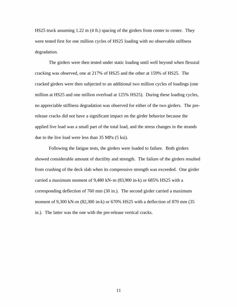
11

HS25 truck assuming 1.22 m (4 ft.) spacing of the girders from center to center. They

were tested first for one million cycles of HS25 loading with no observable stiffness

degradation.

The girders were then tested under static loading until well beyond when flexural

cracking was observed, one at 217% of HS25 and the other at 159% of HS25. The

cracked girders were then subjected to an additional two million cycles of loadings (one

million at HS25 and one million overload at 125% HS25). During these loading cycles,

no appreciable stiffness degradation was observed for either of the two girders. The pre-

release cracks did not have a significant impact on the girder behavior because the

applied live load was a small part of the total load, and the stress changes in the strands

due to the live load were less than 35 MPa (5 ksi).

Following the fatigue tests, the girders were loaded to failure. Both girders

showed considerable amount of ductility and strength. The failure of the girders resulted

from crushing of the deck slab when its compressive strength was exceeded. One girder

carried a maximum moment of 9,480 kN-m (83,900 in-k) or 685% HS25 with a

corresponding deflection of 760 mm (30 in.). The second girder carried a maximum

moment of 9,300 kN-m (82,300 in-k) or 670% HS25 with a deflection of 870 mm (35

in.). The latter was the one with the pre-release vertical cracks.

12

3. TESTS OF AASHTO TYPE III GIRDER

The overall experimental program consisted of static and fatigue tests of two full-

size AASHTO prestressed concrete girders. This chapter presents the details of the tests

of an AASHTO Type III girder.

3.1. Description of Test Specimen

The AASHTO Type III girder tested in this investigation was 19.95 m (65 ft. 5 ½

in.) long and was produced and donated by Bayshore Concrete Products Corporation,

Cape Charles, Virginia.

When the girder was delivered, there were three transverse cracks in the girder.

One crack was located at 2.0 m (6 ft. 8 in.) from the midspan toward one end of the

girder. It crossed the entire top flange and extended 660 mm (26 in.) downward toward

the bottom flange. The second crack was located at 1.8 m (5 ft. 11 in.) from the midspan

toward the other end of the girder. It also crossed the top flange and extended all the way

to the top of the bottom flange, about 787 mm (31 in.). On the same end of the girder,

there was another smaller crack at 3.7 m (12 ft.) from the midspan. This third crack

extended 559 mm (22 in.) downward from the top of the girder on one side, crossed the

top flange, and extended 203 mm (8 in.) downward on the opposite face.

The cracks were very fine and barely visible. If the cracks had not been marked

previously at the prestressing plant, they would be virtually impossible to identify.

Except for these pre-existing cracks, the girder was whitewashed to make new cracks

more visible during testing.

Figure 3.1 shows the cross-sections of the girder. The girder was prestressed

with thirty four (34) ½-in. low-relaxation strands initially tensioned to 138 kN (31 kips)

13

7"

16"

4 1/2"

7 1/2"

22"

7"

7 1/2"

1'-7"

4 1/2"

7"

5 1/4"

3"

9 SP.@2"=1'-6"

2"2 1/4" 1 3/4" (typ.)

2 1/4" (typ.)

7 Sp.@2'=1'-2"

7"

5 SP.@2"

2'-2"

AASHTO TYPE III GIRDER

STRANDS @ MID-SPAN STRANDS @ ENDS

5 1/2" 5 1/4" 2 STRAIGHT STRANDS

12 STRAIGHT STRANDS

22 STRAIGHT STRANDS

Note: 1ft. = 0.305 m; 1 in. = 25.4 mm

Figure 3.1 AASHTO Type III Girder (1 in. = 25.4 mm)

each. Twenty-two of the tendons were straight, and the remaining 12 were draped with

hold-down points at 1.85 m (6 ft. 1 in.) on each side of the midspan. In the top flange of

the girder, there were two additional straight prestressing tendons initially tensioned to

13.3 kN (3 kips) each. These two strands were used primarily to support the stirrups.

12 DRAPED STRANDS 12 DRAPED STRANDS

14

Stirrups were made of No. 13 metric bars (#4 bars). At each end of the girder,

there were six stirrups spaced at 102 mm (4 in.) on centers with the first stirrup being

placed at 76 mm (3 in.) from the end of the girder. The remaining stirrups were spaced at

0.61 m (2 ft.) on centers. The upper loop of each stirrup projected about 102 mm (4 in.)

above the top of the girder to enhance composite action between the girder and the cast-

in-place concrete deck.

Since the girder was tested without a cast- in-place concrete deck, the upper

portion of the stirrup located at the midspan of the girder was cut away so as to provide a

loading area for the actuator. At this location, a steel plate, 406 x 508 x 25.4 mm (16 x

20 x 1 in.), was placed and leveled with a Hydrostone mix.

The cross-sectional properties of the girder are given in Table 3.1, in which yb is

the distance from the centroidal axis to the bottom fiber, I is moment of inertia, Sb is

section modulus with respect to the bottom fiber, and St is section modulus with respect

to the top fiber.

Table 3.1 Cross-sectional Properties of AASHTO Type III Girder

Area (in.2) yb (in.) I (in.4) Sb (in.3) St (in.3)

560 20.3 125,390 6,186 5,070 Note: 1 in. = 25.4 mm

The 28-day concrete strength specified for the Type III girder was 44.8 MPa

(6,500 psi), and a concrete mixture with water-cement ratio of 0.36 was used for the

girder. The mix proportion of the concrete is shown in Table 3.2.

It was reported by the producer that the unit weight of the concrete was 2,425

kg/m3 (151.4 pcf), the slump was 127 mm (5 in.), the air content was 3.5%, and the

concrete temperature was 72°F after mixing. After curing under the normal production

15

procedure, the compressive strength of the concrete was reported by the producer as

shown in Table 3.3.

Table 3.2 Concrete Mix Proportion for Type III Girder

Material Weight (lbs per yd3) Yield (ft3) Lehigh Type III Cement 564 2.87

Mineral Admixture 188 1.03 Solite 1,193 7.35

Vulcan Materials #67 1,873 10.07 Water 270 4.33

Total Air (%) 3.0 ± 2.0 1.35 Note: 1 lb/yd3 = 0.593 kg/m3; 1 ft3 = 0.0283 m3 27.00

Table 3.3 Compressive Strength of Concrete for Type III Girder

Age (days) 1 7 28 Comp. Strength (psi) 5,476 6,962 7,698

Note: 1 MPa = 145 psi or 1 ksi = 6.895 MPa

3.2 Test Set-Up

The girder was supported by elastomeric bearing pads centered at 171 mm (6 ¾

in.) from each end of the girder, creating a simple span of 19.6 m (64 ft. 4 in.) for the test.

The bearing pads were 559 x 229 x 64 mm (22 x 9 x 2.5 in.) before any loading. Each

elastomeric bearing pad was placed between two 25.4 mm (1 in.) thick steel plates. The

top plate was 279 x 762 mm (11 x 30 in.) and the bottom one was 559 x 762 mm (22 x 30

in.). The plates were used to protect the surface of the bearing pads and for better

distribution of load. To prevent any longitudinal movement of the girder during fatigue

loading, two threaded rods were fastened to the bottom plate and a hand-tightened nut

was placed above the top plate. This assembly can be seen in Figure 3.2. Beneath each

support was a reinforced concrete reaction block that was bolted to the laboratory floor.

These 1.23 x 1.23 x 0.61 m (4 x 4 x 2 ft.) blocks, combined with the bearing pads and

16

plates, provided approximately 0.72 m (2 ft.-4 ½ in.) clearance between the bottom of the

girder and the laboratory floor.

Figure 3.2 Bearing Pad Support Assembly

The loading frame was designed to carry an upward axial load of 2,669 kN (600

kips) which was chosen as the design load in order to accommodate the 1,779 kN (400

kips) fatigue capacity of the actuator. The frame, shown in Figure 3.3, consists of two

W30 x 108 columns that support two W36 x 182 reaction beams. The frame was

anchored to the laboratory floor at a location such that the actuator would apply the load

at the midspan of the girder. The design and fabrication of the test frame has been

described in detail by Ellen (2000) and Longo (2000).

17

Figure 3.3 Load Frame for Girder Testing

All the static and fatigue load testing of this specimen was performed using a

MTS actuator with a 1,984 kN (446 kips) fatigue capacity and 1,016 mm (40 in.) stroke.

During the testing, both the load and displacement controls of the actuator were used. A

steel plate of 559 x 508 x 25.4 mm (22 x 20 x 1 in.) was bolted to the lower end of the

actuator to provide a flat contact surface to distribute the load applied to the girder.

18

3.3 Instrumentation

Load and deflection data were recorded at various times throughout the testing.

The load was measured by the load-cell of the actuator. Deflections were measured by

seven string potentiometers (string pots) attached to the girder, one at the midspan, one

on each side of the bearings at both ends of the girder, and one at each quarter point of

the girder. The string pots at midspan and at the quarter points were bolted to aluminum

angles fastened to the laboratory floor. The strings were then connected, using fishing

wire and hook, to aluminum brackets that had been epoxied to the bottom of the girder.

The connection of the string pots at the bearings was slightly different. Brackets were

epoxied to the sides of the girder, instead of the bottom, and the base of the string

potentiometer was fastened to the concrete pads, rather than the laboratory floor as can be

seen in Figure 3.2. String pots with strokes of 2, 10, 15, and 25 inches were used for the

test. The string pot with the largest stroke was placed at the midspan of the girder where

the largest deflection was expected.

Deflection of the girder due to loading was obtained by subtracting the average of

the four string pot readings at the supports from the string pot reading at the midspan.

The same procedure was applied to find the deflection at the quarter points. The string

potentiometer located on both sides of the girder at the bearings was also monitored to

determine if there was any beam rotation in the transverse direction, which could occur if

the load from the actuator was not applied directly through the centroid of the cross-

section of the girder or if the girder was not cast perfectly straight.

Gage points for the mechanical strain gage DEMEC were also applied to the

girder. On one side of the girder, four DEMEC points were epoxied to the bottom flange

19

near the midspan. During initial loading, DEMEC readings were taken in an effort to

determine first cracking in the bottom flange of the girder and thus the corresponding

cracking load. The gage length between the DEMEC points was 76.2 mm (3 in.) and

each division of the DEMEC gauge measured a strain of 15.8 x 10-6.

3.4 Test Procedure

The overall test program consisted of an initial static loading, followed by cycles

of service loading (with intermittent overloading), and a final ultimate load test. Static

load tests were intended to induce flexural cracking in the girder and to determine its

initial flexural response before and after cracking. Several repetitions of static load tests

were performed in order to obtain accurate initial load-deflection curves of the girder.

Fatigue loading was applied in segments of 100,000 cycles of service loading,

followed by a static load test. After each 200,000 cycles of service loading with the

follow-up static load test, 500 cycles of fatigue overload were applied to the girder with

another follow-up static load test. Load-deflection curves were obtained before and after

each 500 cycles of overload.

After the fatigue test, the girder was tested to failure to determine its load carrying

capacity and to observe its behavior. Table 3.4 shows the loading history for the girder.

3.4.1 Tests for Initial Cracking

Static 0-A was the initial test of the girder to induce the flexural cracks. Before

each static load test, the initial readings of potentiometers were recorded so that the

displacement of the girder could be determined during and after the test. The load was

applied slowly with displacement control at the rate of 0.25 mm/sec.(0.01 in./sec.) in

increments of 5.08 mm (0.2 in.) of displacement to ensure that the initial cracking could

20

Table 3.4 Loading History for Type III Girder

TYPE OF TEST

LOADING TYPE

LOAD RANGE (kips)

NUMBER OF CYCLES

TOTAL NUMBER OF FATIGUE CYCLES

Static 0-A 0 - 140 1 0 Static 0-C 0 - 140 1 0

Static 0-D * 0 - 110 1 0 Static 0-E * 0 - 115 1 0 Static A-1* 0 - 140 1 0 Static A-2 * 0 - 145 1 0 Static A-3 * 0 - 140 1 0

TEST FOR INITIAL

CRACKING

Static A-4 0 - 140 1 0 Service 26 - 107 100,000 100,000 Static B 0 - 140 1 100,000 Service 26 - 107 100,000 200,000 Static C 0 - 140 1 200,000 Overload 26 - 152 500 200,500 Static D 0 - 150 1 200,500 Service 26 - 107 100,000 300,500 Static E 0 - 150 1 300,500 Service 26 - 107 100,000 400,500 Static F 0 - 150 1 400,500 Overload 26 - 152 500 401,000 Static G 0 - 150 1 401,000 Service 26 - 107 200,000 601,000 Static H 0 - 150 1 601,000 Overload 26 - 152 500 601,500 Static I 0 - 150 1 601,500 Service 26 - 107 200,000 801,500 Static J 0 - 150 1 801,500

Overload 26 - 152 500 802,000 Static K-1 * 0 - 150 1 802,000 Static K-2 0 - 150 1 802,000

Service 26 - 107 200,000 1,002,000 Static L 0 - 150 1 1,002,000 Overload 26 - 152 500 1,002,500

FATIGUE TEST

Static M 0 - 150 1 1,002,500 Static N 0 - 75 1 1,002,500 Static O 0 - 109 1 1,002,500 Static P 0 - 133 1 1,002,500 Static Q 0 - 147 1 1,002,500 Static R 0 - 156 1 1,002,500 Static S 0 - 172 1 1,002,500 Static T 0 - 182 1 1,002,500 Static U 0 - 191 1 1,002,500 Static V 0 - 204 1 1,002,500

ULTIMATE LOAD TEST

Static W 0 - 196 1 1,002,500 * Applied load was either reached and then unloaded, or not quite reached. Cracks were not marked.

Note: 1 kip = 4.448 kN

21

be observed. After each load increment, the specimen was carefully surveyed for any

flexural cracks.

When the load reached about 596 kN (134 kips), a few fine cracks were observed

on the bottom face of the girder which extended partially into the bottom flange. To

ensure that the cracks were fully developed, the load was increased to 623 kN (140 kips)

and the cracks were marked with black permanent markers. The magnitude of the load

was also recorded at the tip of the crack. In all the static load tests, the maximum crack

length, the maximum crack width, the locations where cracks occurred, the average crack

spacing on the side face, and the average crack spacing on the bottom face of the girder

were all measured and recorded.

After the first static load test and a review of the data file, it was determined that

recording data at small increments of deflection produced too many data points. So a

trial test was conducted to acquire data at every load increment of 8.9 kN (2 kips) and it

proved to be more efficient. So the Static 0-C test was performed to ensure that the

girder was sufficiently cracked, using the revised procedure. The string potentiometer

readings were recorded prior to the static test and 24 hours thereafter.

Two additional static load tests (Static 0-D and Static 0-E) were performed to

determine the load at which the cracks reopened. Twenty four hours prior to Static 0-D

load test, DEMEC points were epoxied around two of the larger cracks on one side of the

girder. Instead of displacement control, load control was used to apply the load with an

increment of 44.5 kN (10 kips) at the rate of 4.45 kN (1 kip) per second. However, it was

found that the loading rate was too rapid to allow enough DEMEC measurements to be

made. So the load increment was reduced to 4.45 kN (1 kip) for Static 0-E load test.

22

For the rest of the static load tests, load was applied slowly rather than at a

specific rate in order to ease the collection of load-deflection data. After each desired

load level was reached, either the load was held for crack marking or unloading followed

immediately. Load-deflection data were collected at every 8.9 kN (2 kips) load

increment.

Due to the need to repair the hydraulic system for the actuator, Static A-1, A-2, A-

3, and A-4 tests were performed 43 days after the initial static load tests. Static A-1, 2, 3,

and 4 were four repetitive tests. On the 4th test (Static A-4), the desired load of 623 kN

(140 kips) was held for crack marking and measurement. In total, eight static load tests

were performed before the beginning of fatigue testing.

3.4.2 Fatigue Test

The girder was tested under fatigue loading without a composite deck. The

fatigue load was applied at midspan as a point load at one cycle per second. This loading

frequency made efficient use of the hydraulic system and avoided resonance with the

natural frequency of the test specimen. The magnitude of the cyclic load varied from

116 kN (26 kips) to 476 kN (107 kips). The lower limit load produced the same moment

at midspan as a composite deck of 2.44 m (8 ft.) wide and 203 mm (8 in.) thick. The

upper limit load would produce a nominal bottom fiber stress of 1.81 MPa (263 psi) at

the midspan of the composite girder (i.e., the test girder with a hypothetical deck), which

is equal to the design stress of 0.25 'cf MPa (3 '

cf psi) used by NCDOT. The

corresponding concrete stress at the bottom layer of prestressing strands would be 1.72

MPa (249 psi) as shown in Figure 3.4. (The corresponding nominal bottom fiber stress in

the test girder would be 1.90 Mpa (276.2 psi) or 0.26 'cf MPa (3.15 '

cf psi.)

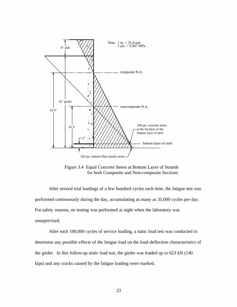
23

8" slab

45" girder

20.3"

36.9"

composite N.A.

noncomposite N.A.

263 psi. bottom fiber tensile stress

249 psi. concrete stressat the location of thebottom layer of steel

2"

bottom layer of steel

Note: 1 in. = 25.4 mm 1 psi. = 0.007 MPa

Figure 3.4 Equal Concrete Stress at Bottom Layer of Strands for both Composite and Non-composite Sections After several trial loadings of a few hundred cycles each time, the fatigue test was

performed continuously during the day, accumulating as many as 35,000 cycles per day.

For safety reasons, no testing was performed at night when the laboratory was

unsupervised.

After each 100,000 cycles of service loading, a static load test was conducted to

determine any possible effects of the fatigue load on the load-deflection characteristics of

the girder. In this follow-up static load test, the girder was loaded up to 623 kN (140

kips) and any cracks caused by the fatigue loading were marked.

24

After each 200,000 cycles of service loading, the girder was subjected to a fatigue

overload test for 500 cycles at one-half cycle per second. The load varied from 116 kN

(26 kips) to 676 kN (152 kips). The overload test represented the effect of over-weight

vehicles allowed to use a bridge with special permit issued by NCDOT, which is based

on 75 percent of the ultimate strength of the girder with a composite deck. After each

500 cycles of overload test, a static load test was again performed with the girder being

loaded up to 667 kN (150 kips) in order to determine any possible effects of the overload

on the load-deflection behavior of the girder. At the load of 667 kN (150 kips), any new

cracks caused by the cyclic overload test were also marked for record.

The above test sequence was continued until a total of 1,002,500 cycles of fatigue

loadings were reached.

3.4.3 Ultimate Load Test

After the fatigue test was completed, the girder was tested to failure under static

load. In order to best document the behavior of the girder prior to failure, several static

load tests were performed at increasing load levels by progressively increasing the

actuator displacement. Table 3.5 shows the test sequence and the load range as well as

the displacement of the actuator.

The load was applied using displacement control, and the loading rate was varied

such that the desired deflection was obtained in about two minutes each time. Data were

recorded every half second for all the loading and unloading cycles.

The girder was loaded and unloaded nine times (Static N to Static V) before it

reached failure. In the interest of safety, cracks on the bottom face of the girder were not

marked, but all cracks on both side faces were marked. On the 10th loading (Static W),

25

Table 3.5 Ultimate Load Test for Type III Girder

LOAD TEST

LOAD RANGE

(kips)

DISPLACEMENT OF ACTUATOR

(in.) STATIC N 0 - 75 1.0 STATIC O 0 - 109 1.5 STATIC P 0 - 133 2.0 STATIC Q 0 - 147 2.3 STATIC R 0 - 156 2.5 STATIC S 0 - 172 3.0 STATIC T 0 - 182 3.5 STATIC U 0 - 191 4.0 STATIC V 0 - 204 5.0 STATIC W 0 - 196 <5.0

Note: 1 kip = 4.448 kN; 1 in. = 25.4 mm

the concrete on the top flange of the girder crushed at midspan, resulting in failure of the

girder.

3.5 Test Results

3.5.1 Tests for Initial Cracking

Crack Development — As indicated in Table 3.4, static tests were repeated eight

times in this phase of the test program. During the first static test, flexural cracks were

observed on the bottom of the girder extending slightly into the bottom flange when the

applied load reached 596 kN (134 kips). After the load was increased to 623 kN (140

kips), the initial cracks were extended further into the bottom flange and some new

cracks were developed. The cracks were located within 0.9 m (3 ft.) on each side of the

midspan. Crack spacing ranged from 178 to 305 mm (7 to12 in.) with an average of

about 254 mm (10 in.). No crack width exceeded 0.05 mm (0.002 in.) and the longest

crack extended 305 mm (12 in.) into the web from the bottom of the girder.

26

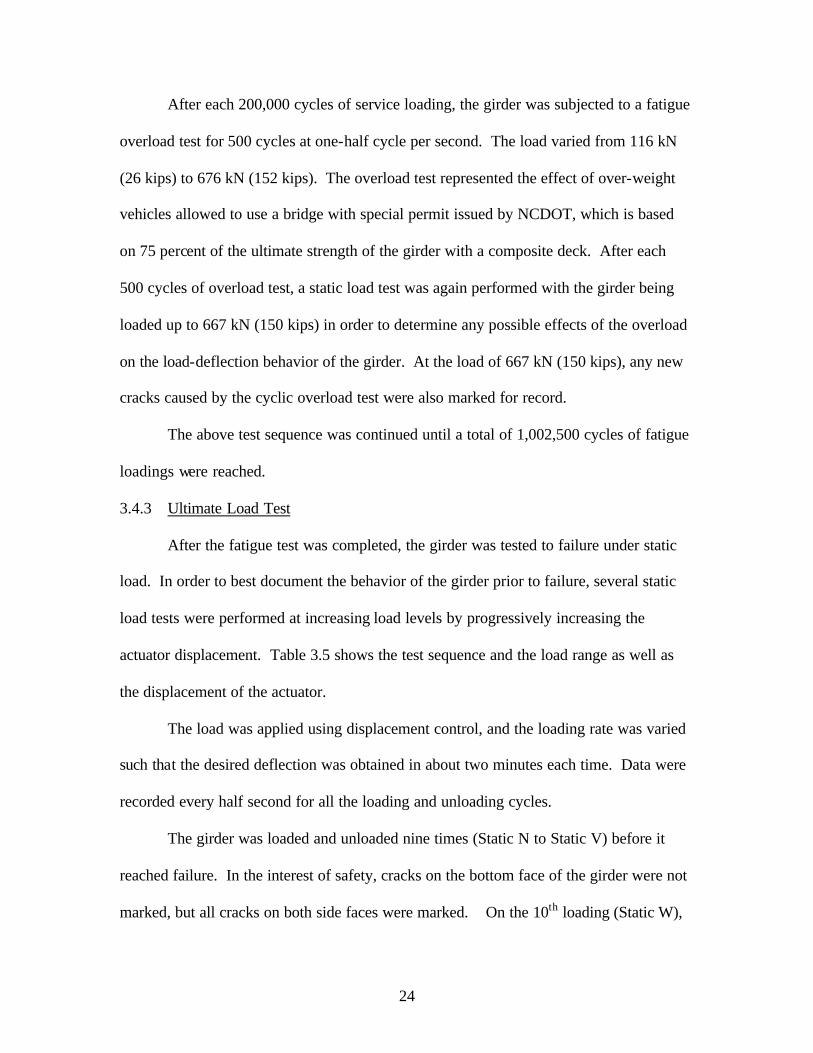
In the second static load test, some of the previously developed flexural cracks

reopened when the applied load reached 507 kN (114 kips); and as the loading increased,

all the existing cracks reopened. When the load reached 623 kN (140 kips), several of the

existing cracks propagated slightly, and several new cracks were discovered. Still no

cracks exceeded 0.05 mm (0.002 in.) in width, but the crack spacing decreased. The

average crack spacing was about 178 mm (7 in.), and all the cracks were located within

1.3 m (4.25 ft.) on each side of the midspan. Figure 3.5 shows the largest cracks after the

second test.

Figure 3.5 Cracks after Static Load 0-C

During the third and the fourth static tests, it was observed that the principal

flexural cracks began to reopen when the applied load reached 446 kN (100.2 kips).

After the eight static tests, the crack width under the load of 623 kN (140 kips) increased

and it varied from 0.13 to 0.18 mm (0.005 to 0.007 in.). The crack spacing remained

27

virtually the same and varied from 152 to 178 mm (6 to 7 in.). The longest crack

extended 381 mm (15 in.) from the bottom of the girder into the web.

Deformation and Stiffness — Prior to the initial flexural cracking, the girder

behaved elastically as shown by the load-deflection curve in Figure 3.6. For each of the

eight static load tests, the load-deflection curve were virtually the same prior to the

opening of the flexural cracks. From the load-deflection curve, it can be seen that the

slope of the curve is 76.4 kips/in. (13.37 kN/mm). Therefore the flexural stiffness of the

girder can be calculated as

EI = (76.4) L3/48 = (76.4) (64.3)3(1728)/48

= 731 x 106 kips- in2 (2,098 x 109 kN-mm2)

where E is the modulus of the concrete, I is the moment of inertia of the girder and L is

the span of the girder. Since I = 125,390 in4 (52,162 x 106 mm4), then

E = 731 x 106/125,390 = 5.83 x 103 ksi. (40.2 GPa).

According to the ACI 318 Code (1999), the modulus of the concrete can also be

estimated as

E = 33γ1.5 'cf

where γ = unit weight of concrete = 151.4 pcf (2,425 kg/m3) and fc' is the 28-day

compressive strength of the concrete = 7,698 psi (53 MPa). Therefore,

E = 5.39 x 103 ksi. (37.2 GPa).

This estimated value of E based on the ACI formula compares quite well with the value

of E obtained from the stiffness of the girder.

28

29

In terms of the permanent deformation, the girder had an initial camber of 29.5

mm (1.16 in.) before the static tests. After the tests, the camber was measured to be 24.4

mm (0.96 in.), representing a loss of 5.1 mm (0.2 in.) in camber.

Flexural Modulus — Knowing the load that causes the initial flexural cracks and

the load that causes the cracks to reopen, one can determine the flexural modulus of the

girder and its effective prestress at the time of testing. During the first and the second

static tests, it was observed that the first flexural cracking occurred when the applied load

was 596 kN (134 kips) and the cracks reopened at the load level of 507 kN (114 kips).

However, it is generally difficult to detect minute cracks in the bottom of the girder by

visual observation. Therefore the above indicated load levels may not be accurate and it

is desirable to examine the load-deflection curve to determine where non-linearity of the

curve begins. From the load-deflection curve shown in Figure 3.6, it appears that better

estimates of the two load levels in question are 556 kN (125 kips) and 436 kN (98 kips)

respectively.

The difference between the two load levels, i.e., ∆P = 556 – 436 = 120 kN (27

kips), represents the load carried by the girder due to the flexural modulus of the

concrete. Since the midspan moment produced by ∆P is

∆M = (∆P)L/4 = 27(64.3)(12)/4 = 5,208 kip- in

and the section modulus for the bottom fiber of the girder is Sb = 6,186 in3, therefore the

flexural modulus of the concrete at the time of testing would be

fr = ∆M/Sb = 5,208/6,186 = 0.842 ksi = 842 psi (5.81 MPa).

30

According to the ACI 318 Code (1999), fr = 7.5 'cf , and by substituting fc

' =

7,698 psi (53 MPa), one obtains fr = 658 psi (4.54 MPa) which is 22% lower than the

value of 842 psi (5.81 MPa) obtained above.

Effective Prestress — Since the flexural cracks reopened at 436 kN (98 kips), one

can determine the effective prestress of the girder at the time of testing. Let F = effective

prestress, fd = bottom fiber stress at midspan due to the dead load of girder, and fa =

bottom fiber stress at midspan due to the applied load of 436 kN (98 kips). Then

–F/A – Fe/S b + fd + fa = 0

in which A = cross-sectional area of girder = 560 in.2 (3,613 cm2),

e = eccentricity of prestressing force at midspan = 12.34 in. (31.34 cm),

Sb = section modulus for bottom fiber = 6,186 in.3 (101,370 cm3),

Md = midspan moment due to dead load of girder = 304.6 ft-kips (413 kN-m),

Ma = midspan moment due to applied load = 1,576 ft-kips (2,138 kN-m).

Then fd = 304,600 x 12 / 6,186 = 591 psi (4.08 MPa)

and fa =1,576,000 x 12 / 6,186 = 3,057 psi (21.10 MPa).

Therefore – F/560 – F(12.34)/6,186 + 591 + 3,057 = 0.

From the above equation, the effective prestress is found to be

F = 964,824 lbs = 964.8 kips (4,291 kN).

Since the initial tension for each of the 34 strands was 137.9 kN (31 kips), the

total initial prestress would be Fi = 34 x 31 = 1,054 kips (4,688 kN). So the loss of

prestress at the time of testing would be 9%.

31

3.5.2 Fatigue Test

Crack Development — During the fatigue test under service loading, crack

development was very limited. After 100,000 service load cycles, no new cracks were

found and crack propagation was minimal. After the second 100,000 service load cycles,

still no new cracks were identified but some cracks propagated 13 to 102 mm (0.5 to 4

in.). Much more significant cracking occurred under the first 500 cycles of overloading.

During the Static Load Test D (see Table 3.4), many new cracks were observed and some

cracks propagated as much as 178 mm (7 in.). Maximum crack length and crack width

increased, while average crack spacing decreased to 165 mm (6.5 in.).

All subsequent service load cycles caused minimum effect on crack development.

The second overloading cycle was much less detrimental than the first. Additional

cracks propagated up to 178 mm (7 in.) and the cracks existed in the central 5.2 m (17 ft.)

portion of the girder. The remaining three overloading cycles also had minimal effect on

crack development. At the end of the fatigue test, cracks in the girder can be

characterized as follows:

(1) The maximum crack length was 546 mm (21.5 in.), well into the web of the girder.

(2) Cracks developed in the lower part of the girder within a

distance of 5.8 m (19 ft.) centered about the midspan. (3) The maximum crack width under a load of 667 kN (150 kips)

was 0.33 mm (0.013 in.). (4) The average crack spacing as measured on the sides of the

girder was 140 mm (5.5 in.). (5) On the bottom of the girder, the average crack spacing was

only 76 mm (3 in.).

32

Stiffness and Deformation — All the load-deflection curves obtained during the

fatigue testing were very closely grouped. A select few of these curves are shown in

Figure 3.7. Only the curves from static load tests occurring after overloading sequences

are shown to avoid unnecessary clutter.

It is significant to note that all the curves are virtually parallel, which indicates

that there was no stiffness degradation after the girder was subjected to 1,000, 000 cycles

of service load and 2,500 cycles of overload. The continuous shifting of the load-

deflection curves provides evidence of the gradual, but permanent reduction in the

camber of the girder.

3.5.3 Ultimate Load Test

Crack Development and Ultimate Load — As expected, cracks developed more

extensively during the ultimate load test than during the fatigue testing. While new

cracks were observed, the average crack spacing remained virtually unchanged at

approximately 140 mm (5.5 in.). The initial loadings, Static N – Static R (see Table 3.5),

were lower than what the girder had already experienced. Therefore, no additional

cracking was observed until Static Load S when some cracks propagated as much as 45.7

cm (18 in.) and the maximum crack length reached 58.4 cm (23 in.).

At Static Load S, there were signs of spalling at the pre-existing cracks, which

were marked at the prestressing plant. Small pieces of concrete were falling off, and

crushing was evident. When the deflection was increased to 89 mm (3.5 in.), the spalling

became even more evident. Furthermore, one of the flexural cracks begun to follow the

path of an original crack found at the plant. At Static Load U, more cracks formed and

some cracks extended upward 737 mm (29 in.) from the bottom of the girder.

33

34

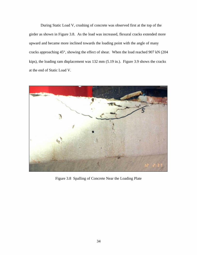
During Static Load V, crushing of concrete was observed first at the top of the

girder as shown in Figure 3.8. As the load was increased, flexural cracks extended more

upward and became more inclined towards the loading point with the angle of many

cracks approaching 45°, showing the effect of shear. When the load reached 907 kN (204

kips), the loading ram displacement was 132 mm (5.19 in.). Figure 3.9 shows the cracks

at the end of Static Load V.

Figure 3.8 Spalling of Concrete Near the Loading Plate

35

Figure 3.9 Cracks after Static Load V

The final static load test, Static Load W, was supposed to reach 153 mm (6 in.) of

actuator displacement. However, when the load on the girder reached only 870 kN (196

kips) and the displacement was less than 127 mm (4.99 in.), the girder collapsed from

extensive crushing of the concrete in the compression zone. So the maximum (ultimate)

load carried by the girder was 907 kN (204 kips) under Static Load V.

Stiffness and Failure Mode — The load-deflection curves for the final ultimate

load test are shown in Figure 3.10. The curves for Static Loads N, O, P, and Q are not

shown since they coincide with that of Static Load R corresponding to the actuator

displacement of 64 mm (2.5 in.). It is noted that all the curves have the same initial

slope, and thus the same stiffness which is roughly 14.6 kN/mm (83.3 kips/in.), with the

exception of the final loading Static Load W. The final curve shows not only a small

decrease in stiffness, but also a further increase in permanent deflection of the girder.

36

37

In addition, it shows that non- linear behavior initiated well before the load reached 444.8

kN (100 kips). The girder collapsed when the load reached 872 kN (196 kips) with a

deflection of slightly less than 127 mm (5 in.). It should be noted that the maximum load

carried by the girder was 907 kN (204 kips) during Static Load V.

Since the girder was tested without a composite deck slab, its failure mode was

sudden and explosive. Failure occurred primarily from crushing of concrete in the

compression zone on one side of the steel loading plate at the location shown in Figure

3.8. As soon as the compression zone was lost, the large force in the prestressing

strands put the remaining concrete area in the web and the bottom flange under a very

high compressive stress which, in turn, caused concrete crushing in those areas. A view

of the girder after failure is shown in Figure 3.11.

Figure 3.11 AASHTO Type III Girder after Failure

38

None of the 34 prestressing tendons in the bottom flange of the girder was

fractured, neither were any of the individual wires in the strands. Bending and unraveling

of the tendons was noted in several locations where the confinement of concrete cover

was lost due to spalling.

39

4. TESTS OF AASHTO TYPE V GIRDER

The overall experimental program consisted of static and fatigue tests of two full-

sized AASHTO prestressed concrete girders. This chapter presents the details of the tests

of an AASHTO Type V girder.

4.1 Description of Test Specimen

The AASHTO Type V girder tested in this investigation was 19.8 m (65 ft.) long

and was also produced and donated by Bayshore Concrete Products Corporation located

in Cape Charles, Virginia.

When the girder was delivered 13 days after casting, there was a camber of 19

mm (0.75 in.). Two cracks were observed in the top flange, located roughly 203 mm (8

in.) on either side of the midspan of the girder and extended down on both faces of the

girder for approximately 610 mm (24 in.) from the top of the girder, or 305 mm (12 in.)

into its web below the top flange. The cracks were virtually invisible. In preparation for

tests, the cracks were marked in red ink and the rest of the girder was whitewashed to

make new cracks more visible during testing.

Typically, Type V girder would be used for spans between 27.4 m (90 ft.) and

36.6 m (120 ft.). However, due to the size limitation of the test floor, a shorter test girder

was used and therefore modifications were made on the number and layout of the

prestressing strands. Figure 4.1 shows the cross-sections of the girder. It can be seen that

only straight strands were used in order to keep the girder from being over-stressed.

Thirty-eight (38) 12.7 mm (1/2 in.) low relaxation prestressing strands were used

in the girder. Two of the strands were pre-tensioned to 4.45 kN (1 kip) for support of

web reinforcement and crack control, and are shown as type “A” strands. Each of the

40

(36) "B" Strands

Note: 1ft. = 0.305 m; 1 in. = 25.4 mm

5"

2'-4"

3"4"

2'-9"

10"

8"

3'-6"

8"

4" 1'-1"

3" (typ.)

3 SP. @ 2"=6"

4 SP. @ 2"=8" (typ.)3"

3 SP. @2"=6"

1'-7"2"

Web Reinforcing

Bottom Flange Bars

(2) "A" Strands

# 4 Bars# 4 Bars

Figure 4.1 AASHTO Type V Girder (1 in. = 25.4 mm)

41

remaining 36 strands were tensioned to 138 kN (31 kips), and are shown as type “B”

strands. Of the 36 fully prestressed strands, four were located in the top flange. Along

with these four prestressed strands, there were four No. 13 metric bars (#4 bars) placed in

the top flange. Two bars extended 10.47 m (34.33 ft.) from each end of the girder and

overlapped at the center of the girder. These bars were used also to help limit possible

cracking that might occur during production of the girder.

Stirrups in the form of 90° bent bars were made of No. 13 metric bars (#4 bars).

At each end of the girder, the stirrups were placed at 50.8 mm (2 in.) spacing for 203.2

mm (8 in.) and increased to 228.6 mm (9 in.) for the next 914.4 mm (36 in.). In the

central portion of the girder, including midspan, the stirrup spacing was approximately

609.6 mm (24 in.). In addition to the stirrups, bottom flange bars were used at the end

sections, but not in the central portion of the girder. The concrete cover for the stirrups

and bars was 50.8 m (2 in.).

The cross-sectional properties of the girder are given in Table 4.1, in which yb is

the distance from the centroidal axis to the bottom fiber, I is moment of inertia, Sb is

section modulus with respect to the bottom fiber, and St is section modulus with respect

to the top fiber.

Table 4.1 Cross-sectional Properties of AASHTO Type V Girder

Area (in2) yb (in) I (in4) Sb (in3) St (in3) 1,013 31.96 521,180 16,307 16,790

Note: 1 in. = 25.4 mm

The 28-day concrete strength specified for the Type V girder was 48 MPa (7,000

psi) and the mix proportion of the concrete as furnished by the producer is shown in

Table 4.2.

42

Table 4.2 Concrete Mix Proportion for Type V Girder

Material Quantity (per yd3) Cement 423 lbs

New Cem 282 lbs #67 Stone 1,873 lbs

Sand 1,209 lbs Water 280 lbs DCIs 2 Gallons

ADVA 50 oz. Daravair 1000 12 oz.

Hycol 21 oz. Note: 1 lb/yd3 = 0.593 kg/m3; 1 fl. oz. = 0.0296 liter

It was reported by the producer that the unit weight of the concrete was 2,412

kg/m3 (150.6 pcf) and the compressive strength of the concrete is as shown in Table 4.3.

Table 4.3 Compressive Strength of Concrete for Type V Girder

Age (days) 1 7 28 Comp. Strength (psi) 4,572 7,293 9,439

Note: 1 MPa = 145 psi or 1 ksi = 6.895 MPa

4.2 Test Set-Up

The girder was supported by elastomeric bearing pads centered at 203 mm (8 in.)

from each end of the girder, creating a simple span of 19.4 m (63.67 ft.) for the test.

Other details of the test set-up were essentially same as described previously in Section

3.2 for the test of Type III girder.

Based on the experience of testing Type III girder, a protective wall of plywood

with a plexi-glass window was placed on each side of the girder at the midspan, as a

safety measure during the ultimate load test. The wall kept any flying debris from

injuring laboratory personnel and the plexi-glass window allowed viewing of the girder

behavior during test.

43

Also for safety reason, three-foot sections of timber cribbing, using 139.7 x 139.7

mm (5.5 x 5.5 in.) lumber, were stacked at the midspan and quarter points under the

girder to keep the girder from damaging the laboratory floor in case of a collapse.

Enough clearance was left between the timber cribbing and the girder so that the girder

could deflect freely until failure.

4.3 Instrumentation

The instrumentation used for the test was essentially same as that described

previously in Section 3.3 for the test of Type III girder. However, in the interest of

safety, a detachable X-Y plotter was used to track the load-deflection curve of the girder

while the girder was being loaded. Knowing the response of the girder in real time

helped to see when failure was imminent. The X-Y plotter was used only during static

load tests after every 200,000 cycles of loading and for the ultimate load test.

4.4 Test Procedure

Type V girder was tested with the same procedure as that for the Type III girder

described in Section 3.4. The girder was tested initially to determine its cracking load,

followed by 1,000,000 cycles of service load (with 2,500 cycles of overload applied

intermittently), and finally the girder was tested for its ultimate load. Table 4.4 shows the

loading history for the girder.

4.4.1 Tests for Initial Cracking

The first static load test, Static A-1, was performed to induce the initial flexural

cracking and the load was applied in 178 kN (40 kips) increments. After each load

increment, the girder was examined closely for cracks. When the load reached 712 kN

(160 kips), smaller load increments were used. Using smaller load increments allowed

44

Table 4.4 Loading History for Type V Girder

TYPE OF TEST

LOADING TYPE

LOAD RANGE

(kips)

NUMBER OF

CYCLES

TOTAL NO. OF FATIGUE CYCLES

Static A-1 0 - 240 1 0 Static A-2 0 - 150 1 0

TEST FOR INITIAL

CRACKING Static A-3 0 - 160 1 0 Service 30 - 186 200,000 200,000 Static B 0 - 240 1 200,000

Overload 30 - 254 500 200,500 Static C 0 - 254 1 200,500 Service 30 - 186 200,000 400,500 Static D 0 - 254 1 400,500 Overload 30 - 254 500 401,000 Static E 0 - 254 1 401,000 Service 30 - 186 200,000 601,000 Static F 0 - 254 1 601,000

Overload 30 - 254 500 601,500 Static G 0 - 254 1 601,500 Service 30 - 186 200,000 801,500 Static H 0 - 254 1 801,500 Overload 30 - 254 500 802,000 Static I 0 - 254 1 802,000 Service 30 - 186 200,000 1,002,000 Static J 0 - 254 1 1,002,000

Overload 30 - 254 500 1,002,500

FATIGUE

TEST

Static K 0 - 254 1 1,002,500 Static L 0 - 254 1 1,002,500 Static M 0 - 276 1 1,002,500 Static N 0 - 286 1 1,002,500 Static O 0 - 296 1 1,002,500 Static P 0 - 300 1 1,002,500 Static Q 0 - 303 1 1,002,500 Static R 0 - 325 1 1,002,500 Static S 0 - 373 1 1,002,500

ULTIMATE LOAD TEST

Static T 0 - 377 1 1,002,500 Note: 1 kip = 4.448 kN

time to examine the girder for the first minute crack which occurred at 925 kN (208 kips).

The crack was marked and labeled at the crack tip as “208A-1”. The load was

45

then increased to 1,068 kN (240 kips) and more general cracks were observed. The

cracks were marked as “240A-1”. Upon unloading, the cracks were closed completely.

The second and third static load tests were conducted to determine the

decompression load and to observe when the cracks would re-open and become visible.

The load was applied at a rate of 4.45 kN/sec (1 kip/sec) and the first crack re-opened

when the load reached 623 kN (140 kips). The load was then increased to 667 kN (150

kips) and any further crack propagation was noted and marked on the beam. Static A-3

test was conducted in the same manner, and the cracks reopened again when the load

reached 623 kN (140 kips). The load was then increased to 712 kN (160 kips) before the

girder was unloaded.

For these static load tests, data was acquired and recorded for every 8.9 kN (2

kips) of load. Each of the seven string potentiometers was read by a data acquisition unit,

and the load and displacement from the actuator were also recorded. New cracks, crack

propagation, crack width, crack length, and spacing were recorded as they occurred

during these static load tests.

4.4.2 Fatigue Test

As before, the girder was tested under fatigue loading without a composite deck.

The fatigue load was applied at midspan as a point load at one cycle per second. The

magnitude of the cyclic load varied from 133 kN (30 kips) to 827 kN (186 kips). The

lower- limit load produced the same moment at midspan as a composite deck of 2.7 m (9

ft.) wide and 213 mm (8 ½ in.) thick. The upper- limit load would produce a bottom fiber

concrete stress of 2 MPa (291 psi) at midspan of the composite girder (i.e., the test girder

with a hypothetical deck), which is equal to the design stress of 0.25 'cf MPa (3 '

cf psi)

46

used by NCDOT. The corresponding concrete stress at the bottom layer of prestressing

strands would be 188 MPa (273 psi) as shown in Figure 4.2. (The corresponding nominal

bottom fiber stress in the test girder would be 2.1 MPa (301 psi) or 0.26 'cf MPa

(3.11 'cf psi.)

48.1"

composite N.A.

noncomposite N.A.

bottom layer of steel

Note: 1 in. = 25.4 mm 1,000 psi. = 6.895 MPa

3"

32"

63" Girder

291 psi bottom fiber tensile stress=cf '3

TARGET STRESS = 273 psi concrete stressat the location of thebottom layer of steel

Figure 4.2 Equal Concrete Stress at Bottom Layer of Strands

for both Composite and Non-composite Sections Based on the experience of the previous test for Type III girder, the fatigue load

was applied continuously during the day, accumulating approximately 30,000 cycles per

47

day, with some days approaching 60,000 cycles. No testing was performed at night when

the laboratory was unsupervised.

After the first 200,000 cycles of service loading, a static load test was conducted

to determine any possible effects of the fatigue load on the load-deflection characteristics

of the girder. In this follow-up static load test, the load was increased up to 1,068 kN

(240 kips) and any new cracks caused by the fatigue loading were marked and recorded.

The girder was then subjected to the first fatigue overload test for 500 cycles at

one-half cycle per second. The load varied from 133 kN (30 kips) to 1,130 kN (254

kips). The latter represented the effect of over-weight vehicles allowed to use a bridge

with special permit issued by NCDOT based on 75 percent of the ultimate strength of the

girder with a composite deck. After 500 cycles of the overload test, a static load test was

again performed with the girder being loaded up to 1,130 kN (254 kips). The load-

deflection behavior of the girder was measured and any new cracks caused by the cyclic

overload test were also marked and recorded.

The above test sequence was continued four more times until a total of 1,000,000

cycles of service load and 2,500 cycles of overload were completed.

4.4.3 Ultimate Load Test

After completion of the 1,002,500 cycles of fatigue loading, the girder was

subjected to the ultimate load test. Table 4.5 shows the test sequence, the load range, and

the displacements of the actuator and the girder.

Initially, the girder was loaded using load control at a rate of 445 kN/min (100

kips/min) for load levels below yield. Six tests involving loading and unloading were

conducted, Static L through Static Q, with increasing load up to 1,348 kN (303 kips).

48

While the load was held at this level, the X-Y plotter showed that the girder was

deflecting without any additional load being applied. At this point, the girder was

unloaded.

Table 4.5 Ultimate Load Test for Type V Girder

ULTIMATE LOAD

LOAD RANGE

ACTUATOR DISPLACEMENT

GIRDER DISPLACEMENT

TEST (kips ) (in.) (in.) L 0 - 254 1.45 1.39 M 0 - 276 1.70 1.63 N 0 - 286 1.89 1.81 O 0 - 296 2.16 2.07 P 0 - 300 2.26 2.17 Q 0 - 303 2.31 2.22 R 0 - 325 2.91 2.86 S 0 - 373 5.30 5.10 T 0 - 377 6.40 5.98

Note: 1 kip = 4.448 kN; 1 in. = 25.4 mm

The ultimate load test was resumed the following day, using displacement control

at a rate of 10 mm/min (0.4 in./min). This corresponded closely to the load-controlled test

conducted the previous day. For Static R test, the displacement was increased up to 74

mm (2.91 in.) when the load reached the pre-set limit of 1,446 kN (325 kips). After

removing the load limit, the testing was started again. For Static S test, the load was

increased to the level that the displacement reached 74 mm (2.91 in.). Then the

displacement was increased in 2.54 mm (0.1 in.) increments until the pre-set

displacement limit of 135 mm (5.3 in.) was reached. As before, the displacement limit

was removed and testing was started again. For Static T test, the load was brought back

again to induce a displacement of 102 mm (4 in.). Then the displacement was increased

in 2.54 mm (0.1in.) increments until failure occurred at 1,677 kN (377 kips) and 163 mm

49

(6.4 in.) of actuator displacement. The failure was explosive, causing crushing of the top

flange of the girder at the midspan.

4.5 Test Results

4.5.1 Tests for Initial Cracking

Crack Development — Static tests to determine the initial flexural cracking were

repeated three times as indicated in Table 4.4. During the first static load test, A-1, the

first flexural crack was observed when the load was at 925 kN (208 kips). When the load

reached 1,068 kN (240 kips), there were four flexural cracks in the bottom flange with

the spacing varying from 356 to 508 mm (14 to 20 in.) and the maximum crack length of

737 mm (29 in.) from the bottom of the girder. The crack width was quite small, in the

order of 0.18 mm (0.007 in.). When the loading was removed, the girder fully recovered

and the cracks were hardly visible.

The second and the third static load tests, A-2 and A-3, were performed to

observe the reopening of the cracks which occurred when the load was 623 kN (140

kips). The tests did not cause any change in the crack properties from the first test A-1.

Deformation and Stiffness — The girder behaved elastically before the initial

cracking as shown by the load-displacement curve A in Figure 4.3. The slope of the

curve is 290 kips/in. (50.8 kN/mm). Therefore the flexural stiffness of the girder can be

computed as EI = (290) L3/48 = (290) (63.67)3(1,728)/48

= 2,695 x 106 kips- in2 (7,735 x 109 kN-mm2)

where E is the modulus of the concrete, I is the moment of inertia of the girder and L is

the span of the girder. Since I = 521,180 in4 (216,810 x 106 mm4), then

E = 2,695 x 106/521,180 = 5.18 x 103 ksi. (35.7 Gpa)

50

51

According to the ACI 318 Code (1999), the modulus of the concrete can also be

estimated as

E = 33γ1.5 'cf

where γ = unit weight of concrete = 150.6 pcf (2,412 kg/m3) and fc' is the 28-day

compressive strength of the concrete = 9,440 psi (65.1 MPa). Therefore,

E = 5.93 x 103 ksi. (40.9 GPa).

This estimated value of E based on the ACI formula is 13.6% higher than the value of E

obtained from the stiffness of the girder. This seems reasonable, considering the fact that

the girder was tested when the concrete was 21 days old.

Flexural Modulus — Knowing the load that causes the initial flexural cracks and

the load that causes the cracks to reopen, one can determine the flexural modulus of the

girder and its effective prestress at the time of testing. During the three static tests, it was

observed that the first flexural cracking occurred when the applied load was 925 kN (208

kips) and the cracks reopened at the load level of 623 kN (140 kips). However, it is

generally difficult to detect minute cracks in the bottom of the girder by visual inspection.

Therefore the above indicated load levels may not be accurate and it is desirable to

examine the load-deflection curve to determine where non- linearity of the curve begins.

From the load-deflection curve shown in Figure 4.3, it appears that the non- linearity

begins at the load level of 712 kN (160 kips), suggesting that the cracks would reopen at

this load level.

The difference between the two load levels, i.e., ∆P = 925 – 712 = 213 kN (48

kips), represents the load carried by the girder due to the flexural modulus of the

concrete. Since the midspan moment produced by ∆P is

52

∆M = (∆P)L/4 = 48(63.67)(12)/4 = 9,168 kip- in. (1.034 x 106 kN-mm)

and the section modulus for the bottom fiber of the girder is Sb = 16,307 in3, therefore the

flexural modulus of the concrete at the time of testing would be

fr = ∆M/Sb = 9,168/16,307 = 0.526 ksi = 526 psi (3.63 MPa).

According to the ACI 318 Code (1999), fr = 7.5 'cf , and by substituting the 28-

day concrete strength fc' = 9,440 psi, fr = 729 psi. By comparison, the above calculated

value of 526 psi based on the load-deflection curve is 28% less than the prediction by the

ACI Code formula. It should be noted that the test was performed before the concrete

age reached 28 days, and therefore the value based on the test is expected to be less than

the prediction by the ACI Code formula.

Effective Prestress — Since the flexural cracks reopened at 712 kN (160 kips),

one can determine the effective prestress of the girder at the time of testing. Let F =

effective prestress, fd = bottom fiber stress at midspan due to the dead load of girder, and

fa = bottom fiber stress at midspan due to the applied load of 712 kN (160 kips). Then

–F/A – Fe/S b + fd + fa = 0

in which A = cross-sectional area of girder = 1,013 in.2 (6,535 cm2),

e = eccentricity of prestressing force at midspan = 20.85 in. (52.96 cm),

Sb = section modulus for bottom fiber = 1,6307 in.3 (267,224 cm3),

Md = midspan moment due to dead load of girder = 536.6 ft-kips (727 kN-m),

Ma = midspan moment due to applied load = 2,547 ft-kips (3,453 kN-m).

Then fd = 536,600 x 12 / 16,307 = 395 psi (2.72 MPa)

and fa =2,547,000 x 12 / 16,307 = 1,874 psi (12.92 MPa).

53

Therefore – F/1,013 – F(20.85)/16,307 + 395 + 1,874 = 0.

From the above equation, the effective prestress is found to be

F = 1,001,300 lbs = 1,001.3 kips (4,453.8 kN).

Since the initial tension for each of the 36 strands was 137.9 kN (31 kips), the

total initial prestress would be Fi = 36 x 31 = 1,116 kips (4,964 kN). So the loss of

prestress at the time of testing would be 10.4%.

4.5.2 Fatigue Test

Crack Development — As shown in Table 4.4, the first segment of 200,000

cycles of fatigue loading was applied after the initial three static load tests. Since the

fatigue load range was from 133.5 kN (30 kips) to 827.7 kN (186 kips) and the upper

limit was less than the maximum load reached in the first static load test, the fatigue

loading had little impact on the crack development of the girder. However, the follow-up

test, Static Load B, was applied to a load of 1,068 kN (240 kips) and new flexural cracks

developed while old cracks extended. The cracks were located within the central 3.66 m

(12 ft.) of the girder and their spacing were reduced to the range of 203 to 254 mm (8

to10 in.). The maximum crack length was increased to 813 mm (32 in.) from the bottom

of the girder. The maximum crack width was 0.4 mm (0.016 in.)

After the first 500 cycles of overloading, Static Load C was executed. Both of

these tests, with load being carried to 1,130 kN (254 kips), had a major influence on the

crack development. New cracks were induced and old crack propagated. The cracks

now occupied the central 4.12 m (13.5 ft.) of the girder. The crack width was measured

to be 0.51 mm (0.02 in.). Though the crack spacing remained the same, the maximum

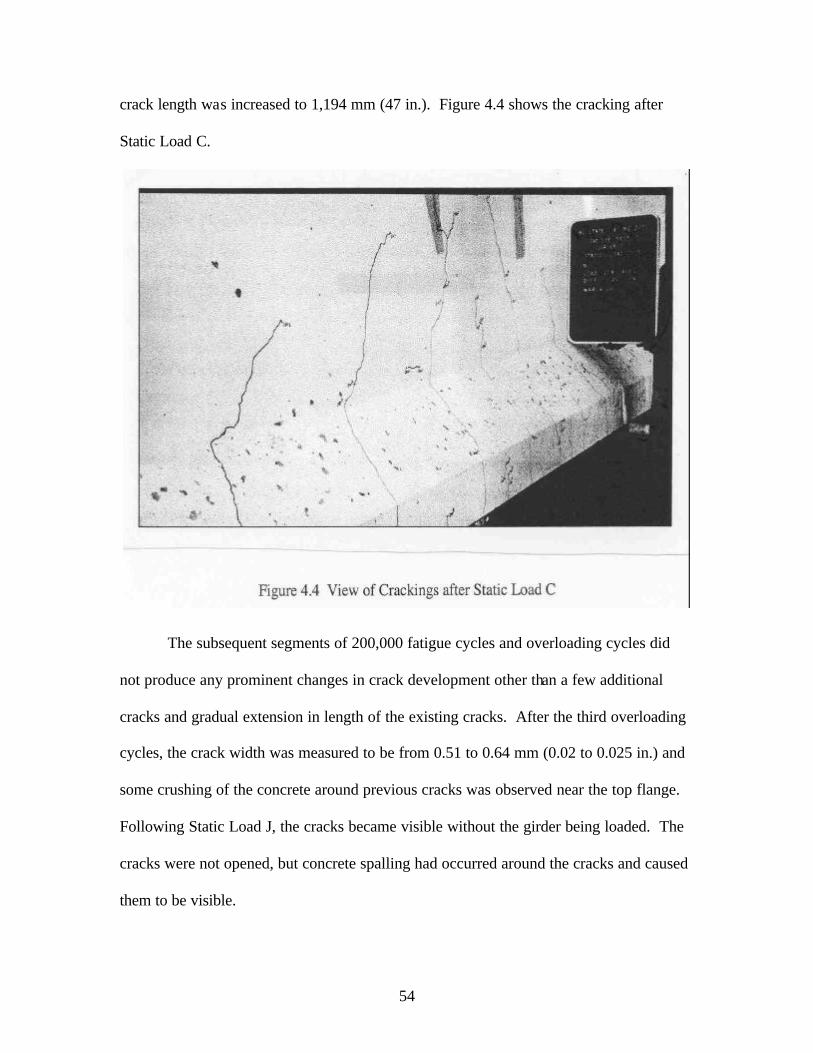
54

crack length was increased to 1,194 mm (47 in.). Figure 4.4 shows the cracking after

Static Load C.

The subsequent segments of 200,000 fatigue cycles and overloading cycles did

not produce any prominent changes in crack development other than a few additional

cracks and gradual extension in length of the existing cracks. After the third overloading

cycles, the crack width was measured to be from 0.51 to 0.64 mm (0.02 to 0.025 in.) and

some crushing of the concrete around previous cracks was observed near the top flange.

Following Static Load J, the cracks became visible without the girder being loaded. The

cracks were not opened, but concrete spalling had occurred around the cracks and caused

them to be visible.

55

Figure 4.5 shows a view of the girder at the end of the fatigue test. Cracking in

the girder at that stage can be characterized as follows:

(1) Crack spacing ranged from 203 to 254 mm (8 to10 in.).

(2) Cracks existed in the central part of 4.12 m (13. ft.) of the girder and remained unchanged during the last eight static tests.

(3) The maximum crack length was 1,194 mm (47 in.) near the

midspan.

(4) The maximum crack width was 0.64 mm (0.025 in.) under a load of 1,130 kN (254 kips).

56

Stiffness and Deformation — As shown in Figure 4.3, curve A is the load-

deflection curve for the initial static load test. Curve C was obtained after the first

overload test which followed the first segment of 200,000 cycles of fatigue test. Curve K

was obtained after the final overload test which was preceded by 1,002,500 fatigue cycles

of service load and overload. It is significant that the three curves are virtually parallel,

which suggests that there was no stiffness degradation due to the fatigue loadings. The

continuous shifting of the load-deflection curves indicates a gradual, but permanent

reduction in the camber of the girder.

4.5.3 Ultimate Load Test

Crack Development and Ultimate Load — As shown in Table 4.5, there were nine

steps (loading and unloading) involved in the ultimate load test with loadings reaching as

high as 1,677 kN (377 kips). As expected, the crack characteristics changed drastically

as more load was applied to the girder. In the first test, L, the load was applied only up to

1,130 kN (254 kips) and therefore no new cracks were observed. In test M, when a load

of 1,228 kN (276 kips) was applied, a crack extended upward and reached the top of the

web while several new cracks as long as 432 mm (17 in.) developed. From test N

through test Q, the applied load was successively increased to 1,348 kN (303 kips),

causing more new cracks with reduced crack spacing. Some existing cracks propagated

as much as 737 mm (29 in.). During test Q, cracking in the concrete was very audible

and, with the load being held at 1,348 kN (303 kips), the girder displacement began to

increase rapidly. At that stage, the crack characteristics can be described as:

(1) The central cracked region of the girder had increased from 4.12 m (13.5 ft.) to 5.03 m (16.5 ft.).

57

(2) New cracks had developed outside the previously cracked region and therefore crack spacing remained basically unchanged at 203 to 254 mm (8 to10 in.).

(3) The longest crack had extended to the top of the web,

i.e.,1,295 mm (51 in.) from the bottom of the girder with the maximum crack width remaining at 0.64 mm (0.025 in.).

The final three tests (R, S, and T) for ultimate load were applied with

displacement control using 2.54 mm (0.1 in.) increments. At 63.5 mm (2.5 in.) of

displacement and 1,335 kN (300 kips) of load, a 457 mm (18 in.) long shear crack

developed in the web of the girder. As the displacement was increased to 68.6 mm (2.7

in.), new shear cracks were formed with the original shear crack extending to the top of

the web as far as 2.13 m (7 ft.) from midspan. When the displacement was increased to

101.6 mm (4 in.), another shear crack occurred with a popping sound and reached as far

away as 2.74 m (9 ft.) from midspan. Finally, when the displacement reached 162.6 mm

(6.4 in.) with load at 1,677 kN (377 kips), failure occurred at a section approximately

0.91 m (3 ft.) from the midspan. At failure, the shear crack spacing was 127 to 178 mm

(5 to 7 in.) and the cracks had spread over the central 8.23 m (27 ft.) of the girder.

Stiffness and Failure Mode — The load-deflection curves for the final ultimate

load tests are shown in Figures 4.6 and 4.7. It is clear that after over 1,000,000 cycles of

fatigue loading, the girder did not suffer any stiffness degradation since all the load-

deflection curves are parallel to each other in the elastic region. However, the fatigue

loading did cause increasing permanent deflections in the girder. Furthermore, in the

final ultimate load test, the girder did lose its elastic behavior at early stages of loading

due to the extensive cracking developed in the girder.

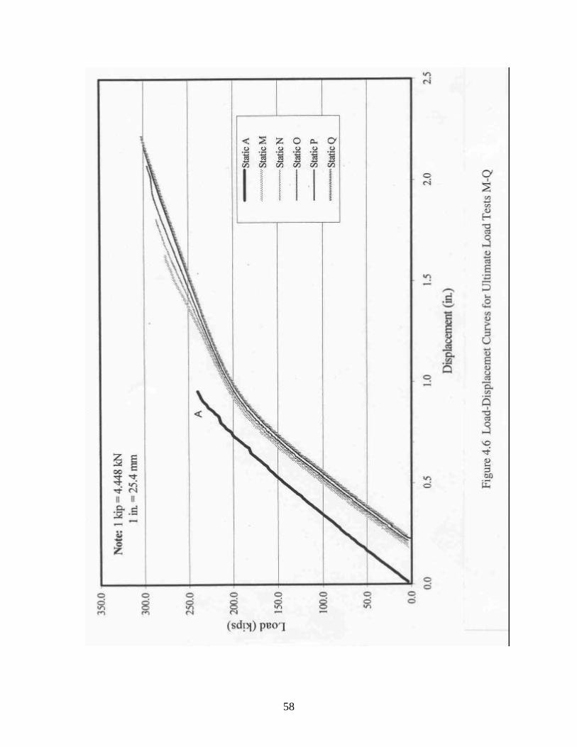
58

59

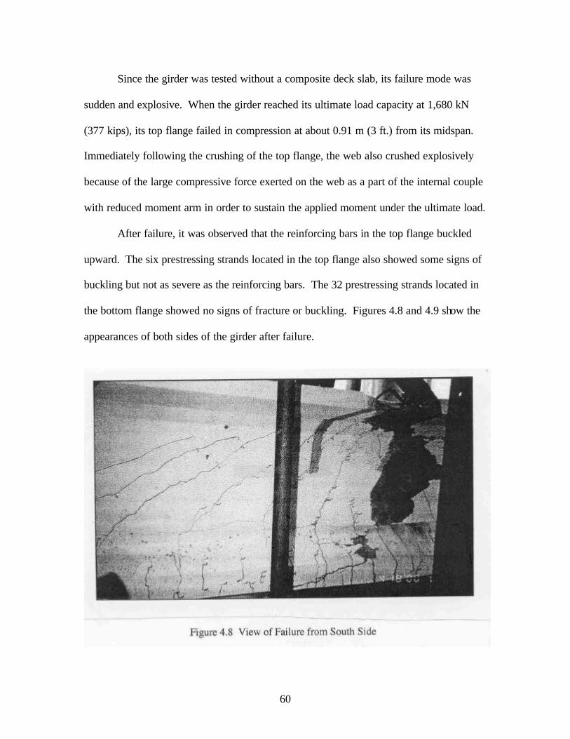
60

Since the girder was tested without a composite deck slab, its failure mode was

sudden and explosive. When the girder reached its ultimate load capacity at 1,680 kN

(377 kips), its top flange failed in compression at about 0.91 m (3 ft.) from its midspan.

Immediately following the crushing of the top flange, the web also crushed explosively

because of the large compressive force exerted on the web as a part of the internal couple

with reduced moment arm in order to sustain the applied moment under the ultimate load.

After failure, it was observed that the reinforcing bars in the top flange buckled

upward. The six prestressing strands located in the top flange also showed some signs of

buckling but not as severe as the reinforcing bars. The 32 prestressing strands located in

the bottom flange showed no signs of fracture or buckling. Figures 4.8 and 4.9 show the

appearances of both sides of the girder after failure.

61

62

5. ANALYTICAL STUDIES 5.1 Introduction

Analytical studies were conducted to model the behavior of the test girders by

using two separate computer programs. The first is a spreadsheet program called

Cracked Beam which was developed by Longo (2000). The second is Response 2000

developed by Bentz (2000). This chapter presents the applications of the two programs

for the analyses of the test specimens. Details of these two computer programs are given

in Appendices A, B, C, and D.

The input and output of both programs will be discussed first, followed by

comparisons of the analytical results. Although the same cross-sectional properties,

prestressing details, and material properties were used in both analyses, each program

required slightly different data for input.

5.2 Analysis of AASHTO Type III Girder

5.2.1 Analysis by Cracked Beam Program

A list of the user inputs for the Cracked Beam analysis is given below. In

addition, the cross-sectional dimensions and the strand layout were also entered as input.

As an illustration, Appendix B shows a computer printout of the Cracked Beam

spreadsheet program.

LIST OF MATERIAL PROPERTIES:

Ultimate tensile strength of 7-wire strand, ƒpu = 1,862 MPa (270 ksi.)

Modulus of elasticity of strand, Es = 196,565 MPa (28,500 ksi.)

Area of strand, Aps (1 tendon) = 98.7 mm2 (0.153 in2)

Jacking force per strand = 214 MPa (31 kips)

63

Prestress losses = 9%

Concrete compressive strength, ƒ’c (girder) = 53.10 MPa (7,700 psi.)

Concrete unit weight, γc (girder) = 2,425 kg/m3 (151.4 lbs/ft3)

Maximum concrete strain at ultimate moment = 0.003

Based on the Cracked Beam analysis, the ultimate moment of the girder was

found to be 4,453 kN-m (3,284 ft-kips). Under this moment, yielding occurred in the

bottom six layers of prestressing strands, according to the stress-strain curve given in the

PCI Handbook (1999) for a Grade 270 strand as shown below:

psspsps Ef εε =≤ :0086.0 (ksi) (5-1a)

007.004.0

270:0086.0−

−=≥ps

psps fε

ε (ksi) (5-1b)

where εps = strain in the prestressing strand fps =stress in the prestressing strand (ksi) Es = Modulus of elasticity of prestressing strand (ksi)

So yielding occurred in all the strands within 305 mm (12 in.) from the bottom of the

girder. The total tensile as well as compressive force in the girder was equal to 5,747 kN

(1,292 kips) under the ultimate moment. Other results for the girder before flexural

cracking are shown in Table 5.1. It should be noted that the applied decompression load

and the applied cracking load were not obtained directly from the analysis. Instead, they

were calculated from the corresponding moments after deducting the dead load moment

of the girder due to self-weight.

The Cracked Beam analysis also showed that the fatigue service load was 480 kN

(108 kips), producing a moment of 2,760 kN-m (2,037 ft.-kips), which is virtually

identical to the actual fatigue service load of 476 kN (107 kips) applied during the test.

64

At the service load, the stress in the bottom layer strands was found to be 1,417 MPa

(205.5 ksi) and 1,436 MPa (208.2 ksi), respectively, for a uncracked and cracked section.

Table 5.1 Results of Analysis for Girder before Flexural Cracking

Load and Moment before Flexural Cracking Decompression Moment 1892.7 ft-kips Applied Decompression Load 98.8 kips Cracking Moment 2253.5 ft-kips Applied Cracking Load 121.2 kips

Stress and Strain under Dead Load Top Fiber Concrete Stress -0.193 ksi Bottom Fiber Concrete Stress -2.897 ksi Top Fiber Concrete Strain -0.0000429 Bottom Fiber Concrete Strain -0.0006423 Bottom Layer Strand Stress 184.4 ksi

Note: 1 kip = 4.448 kN; 1 ft-kip = 1.355 kN-m

To determine the fatigue overload, the stress in the bottom layer strands of a

composite section (i.e., the girder with a composite deck) was analyzed first under 75%

of its ultimate moment. The stress was found to be 1,504 MPa (218 ksi.). The computer

program Cracked Beam was then used to find the required moment in the girder

(noncomposite) that would cause the same stress in the bottom layer strands. The

required moment and the corresponding point load were found to be 3,398 kN-m (2,508

ft-kips) and 609 kN (137 kips) respectively. In contrast, the actual applied load and

moment during the test were 676 kN (152 kips) and 3,727 kN-m (2,749 ft.-kips)

respectively. So the applied fatigue overload was more than the theoretical value by 11%

and the girder was tested more severely than expected.

65

5.2.2 Analysis by Response 2000 Program

The test specimen, AASHTO Type III girder, was also analyzed by using a

computer program called Response 2000 (version 1.0.0). The program is capable of

modeling moment curvature plots, steel and concrete stresses, crack development, and

longitudinal strain, as well as other features. In order to evaluate a specific section of the

girder, such as the midspan, it is necessary to find the ratio of the shear and moment

acting on that section. By using statics to find this ratio at different sections along the

girder, one can determine the behavior of the entire girder. This procedure has been

discussed more fully by Ellen (2000) and certain selected sections of the user's manual

for Response 2000 are given in Appendix D.

Response 2000 allows the user to prescribe any cross-section, but also provides

several common sections preset in the program. Regardless of whether a section is

chosen, or entered manually into the program, the cross-sectional area, section modulus,

moment of inertia of uncracked section, and the location of the neutral axis are all

calculated by the program. Once the cross-section is established, it is necessary to define

the reinforcement. The size, type, and location of prestressing strands are entered into the

program. When the strand characteristics are entered, the prestrain corresponding to the

effective prestress, is entered after allowing for the prestress losses. The prestrain value

used in this analysis was εps = 0.00647.

In addition to defining the prestressing steel, Response 2000 also allows input of

data on shear reinforcement. While the stirrup spacing changes along the length of the

girder, Response 2000 only requires the stirrup spacing at the section under investigation.

66

Initially, the cross-section for an AASHTO Type III girder was selected for

analysis from the predefined menu. After the input for the geometry of the cross-section

and the reinforcement have been made, it was necessary to specify the structural

characteristics of the materials used in the girder. Even though Response 2000 is capable

of calculating material properties, it is possible to override the defaults defined in the

program. The following material properties were entered into Response 2000 as input:

CONCRETE:

Compressive strength = 53.10 MPa (7,700 psi)

Modulus of rupture = 5.81 MPa (842 psi) (based on experimental results)

Peak strain = 0.00229

Maximum aggregate size = 19.1 mm (0.75 in.)

PRESTRESSING STEEL (low-relaxation strands):

Ultimate tensile strength = 1,862 MPa (270 ksi)

Modulus of elasticity = 196,565 MPa (28,500 ksi)

Rupture strain = 0.04

SHEAR REINFORCEMENT:

Yield strength = 414 MPa (60 ksi)

Ultimate tensile strength = 517 MPa (75 ksi)

Modulus of elasticity = 203,462 MPa (29,500 ksi)

Strain at hardening = 0.007

Rupture strain = 0.1

In addition to the selected concrete properties shown above, the Popovics stress-strain

curve (see Collins and Mitchell 1997) for concrete was chosen for the analysis.

67

With all of the properties of the girder inputted into the computer program, a

sectional analysis was performed. Since flexural failure was expected, the analysis was

performed for the midspan section. The ultimate moment of the girder, including the

girder self-weight, was found to be 4,505 kN-m (3,345 ft.-kips). After subtracting the

dead load moment of 413 kN-m (304.6 ft-kips), the required applied point load at failure

was determined as 841 kN (189 kips).

At the ultimate moment, the strain in the concrete was 0.00259 and crushing of

concrete was indicated. As the moment-curvature plot began to fall slightly before

collapse, the concrete strain increased to 0.00273 and then to 0.00290. Prior to concrete

crushing, none of the prestressing steel was yielding. The stress in the strands was 1,637

MPa (237.4 ksi), which increased to 1,659 MPa (240.6ksi) at the cracks. Response 2000

also indicated a stress of 250 MPa (36.2 ksi) in the stirrups before concrete crushing.

After concrete crushing, the stress increased immediately to yielding.

The fatigue overload was also calculated by Response 2000. At 75% of the

ultimate moment of the composite section, the stress in the bottom layer strands was

1,285 MPa (186.3 ksi.). To develop this same stress in the non-composite girder, a

moment of 3,092 kN-m (2,282 ft.-kips) was required. Corresponding to this moment, the

required applied load would be only 547 kN (123 kips). Again, the actual fatigue

overload of 676 kN (152 kips) used during the test exceeded the theoretical value by 24%

and the girder was tested more severely than expected.

After the sectional analysis was performed, Response 2000 was used to evaluate

the full-member response. Due to symmetry, the full response analysis was performed

for one half of the span. The following information was also entered as input.

68

GEOMETRY AND LOADING:

Length of girder subjected to shear = 9,804 mm (385.98 in.)

Constant moment zone on right = 0.00

Constant shear analysis (Point loads were applied)

Moment at left as percentage of right = 0.00%

LEFT SIDE PROPERTIES:

Support at Bottom

RIGHT SIDE PROPERTIES:

Load on continuous beam, load on top

The full-member response provides a plot of shear load versus maximum

deflection, and as with the sectional response, it does not take into consideration the dead

load effect. Therefore, it is necessary to subtract the equivalent applied load due to the

girder weight from the full-member shear load versus deflection curve in order to

compare this curve with the experimental results.

The dead load moment effect was converted to an applied load, as before, using

the static relationship of moment and load for a simply supported beam. An applied load

of 84.2 kN (18.9 kips) would create the same moment at midspan as the dead load of the

girder. Before subtracting this load from the shear load versus deflection plot, the shear

load values must be doubled, since the full response analysis was performed for one half

of the beam length due to symmetry.

After adjusting the loads, the deflection values had to be modified as well.

During the test, the applied load was plotted against the actual displacement of the girder

from its initial cambered position, whereas Response 2000 predicted deflection of the

69

girder as if the girder was level. After adjustments for the displacements were made, the

final applied load versus total deflections plot was then developed which is shown in

Figure 5.1. It can be seen that the cracking load was at 663 kN (149 kips) and the

ultimate load was at 850 kN (191 kips). Under the dead load of the girder, Response

2000 predicted the camber as 28.2 mm (1.11 in.). Including this camber, the total

displacement at failure was 113 mm (4.43 in.). At the ultimate load during the test, the

actual girder deflection was measured as 126 mm (4.96 in.).

5.2.3 Comparisons of Experimental and Analytical Results

Figure 5.1 shows a good comparison between the load versus displacement curves

obtained from the test and from the full member response analysis by Response 2000.

Initially, the experimental curve shows a slightly greater stiffness than the theoretical

curve because the tension stiffening effect of the concrete between the cracks. However,

the experimental curve loses linearity much sooner that the theoretical curve, possibly

because of the effect of fatigue loading. Regardless, the girder fails at a slightly greater

load than that predicted by the computer model. Table 5.2 shows the predicted and

experimental results of the girder at flexural cracking and ultimate load.

Table 5.2 Comparisons for Cracking and Ultimate Loads

Cracking Moment

Cracking Load

Ultimate Moment

Ultimate Load

Method (ft-kips) (kips) (ft-kips) (kips)

Experimental 2,315 125 3,590 204

Cracked Beam Analysis 2,254 121 3,284 185

Response 2000 – Sectional 2,373 129 3,345 189

Response 2000 – Full Member 2,702 149 3,377 191 Note: 1 kip = 4.448 kN; 1 ft-kips = 1.355 kN-m

70

71

As shown in Table 5.2, the theoretical ultimate loads for the girder are less than

the experimental ultimate load, even after 1,002,500 fatigue cycles. So the predictions

are on the conservative side. It should be noted that all the material properties of the

girder used for each analysis were the actual experimentally determined values. For

example, the average cylinder compressive strength and the experimentally determined

concrete tensile strength were used in these programs.

To further compare the results of experiment and analyses, Table 5.3 shows the

stress in the bottom layer strands at each loading stage.

Table 5.3 Comparisons of Stresses in Strands

Stresses in the Bottom Layer Strands (ksi)

Dead Load

Minimum Fatigue Load

Fatigue Service Load

Fatigue Overload

Ultimate Load

Cracked Beam 184.4 188.7 208.2* 218.0 258.0

Response 2000 166.8 171.0 183.9 186.3 240.6 Note: 1 ksi = 6.895 MPa * Based on cracked section analysis. For uncracked section, the stress is 202.4 ksi

According to Cracked Beam analysis, the stress range under fatigue service load

was 134 MPa (208.2 ksi −188.7 ksi = 19.5 ksi), which was increased to 202 MPa (218 ksi

– 188.7 ksi = 29.3 ksi) under fatigue overload. Analysis by Response 2000 resulted in a

stress range of 89 MPa (12.9 ksi) under fatigue service load, and a stress range of 105

MPa (15.3 ksi) under fatigue overload, which are noticeably smaller than those from the

Cracked Beam analysis. This is partly due to the fact that the stress-strain curve of the

prestressing steel was modeled differently in each program. Whereas Cracked Beam

used the PCI stress-strain relationship (1999), Response 2000 used the Ramberg-Osgood

equation found in Collins and Mitchell (1997) as shown below:

72

( )[ ] puCCpf

pfpp fB

AAEf ≤

+

−+=

/11

1

εε (5-2)

where A = 0.025, B = 118, C = 10 for low-relaxation strands with fpu = 270 ksi A = 0.03, B = 121, C = 6 for stress-relieved strands with fpu = 250 ksi

A comparison of the camber and deflection at failure of the girder is shown in

Table 5.4. The camber was predicted within 5% and the deflection at failure was within

15%. A possible reason for the smaller predicted deflection is that the maximum

compressive strain of the concrete was underestimated by Response 2000. If the concrete

strain in the girder exceeded 0.00259 as predicted by Response 2000, then the deflection

would be greater than indicated.

Table 5.4 Comparisons of Camber and Deflection at Failure

Initial Camber (in.)

Deflection at Failure (in.)

Experimental 1.16 5.19

Response – Full Member 1.11 4.43 Note: 1 in. = 25.4 mm

5.3 Analysis of AASHTO Type V Girder

5.3.1 Analysis by Cracked Beam Program

As before, the cross-sectional dimensions, tendon layout, and material properties

are entered first as input. Then the following material properties were entered into the

program.

LIST OF MATERIAL PROPERTIES:

Ultimate tensile strength of 7-wire strand, ƒpu = 1,862 MPa (270 ksi.)

Modulus of elasticity of strand, Es = 196,565 MPa (28,500 ksi.)

73

Area of strand, Aps (1 tendon) = 98.7 mm2 (0.153 in2)

Jacking force per strand = 214 MPa (31 kips)

Prestress losses =10.4%

Concrete compressive strength, ƒ’c (girder) = 65 MPa (9,440 psi.)

Concrete unit weight, γc (girder) = 2,412 kg/m3 (150.6 lbs/ft3)

Maximum concrete strain at ultimate moment = 0.003

Based on the Cracked Beam analysis, the ultimate moment of the girder was

found to be 8,189 kN-m (6,040 ft-kips). To produce this ultimate moment in the girder,

an applied point load of 1,539 kN (346 kips) was required. Under this moment, the stress

in the bottom layer strands was 1,855 MPa (269 ksi). The analysis also found that the

cracking moment of the girder was 5,558 kN-m (4,099 ft-kips) with the corresponding

applied point load being 996 kN (224 kips). In addition, the stress in the bottom layer

strands with the girder supporting the weight of a deck was 1,262 MPa (183 ksi), and the

stress under service load was 1,358 MPa (197 ksi).

To determine the fatigue overload, a composite girder (i.e., the test girder

combined with a deck) was analyzed first by the Cracked Beam program, and the

ultimate moment was found to be 9,923 kN-m (7,319 ft-kips). Under 75% of the ultimate

moment, the stress in the bottom layer stands was 1,531 MPa (222 ksi). The moment that

would produce the same stress in the test girder (non-composite) was 6,195 kN-m (4,569

ft-kips). After subtracting the dead load moment of 727 kN-m (535.6 ft-kips), the

required overload was found to be 1,130 kN (254 kips), which was the same fatigue

overload used during the test.

74

5.3.2 Analysis by Response 2000 Program

The cross-section of the girder was entered first as input. Since the AASHTO

Type V section was not available as a standard shape in the computer program, it was

entered using the user defined menu tab. It was a rather simple step where the widths of

the section at desired heights were entered.

After entering the cross-section geometry, the prestressed and non-prestressed

steels were entered. Since the critical section of the girder was at midspan, only the steel

properties at that section were entered. The stirrups were entered as #4 bars spaced at

610 mm (24 in.) with the concrete cover of 81 mm (3.2 in.) on top and bottom. The only

input value, besides the number and location, of the prestressing strands that needed to be

entered was the prestrain value. This value was 0.00711 based on the jacking force of

138 kN (31 kips), the strand area of 99 mm2 (0.153 in.2), and the modulus of elasticity of

steel of 196,565 MPa (28,500 ksi). Once the steel layout was entered and the girder

cross-section generated, the following material properties were entered into Response

2000 as input:

CONCRETE

Compressive strength = 65 MPa (9,440 psi)

Modulus of rupture = 3.88 MPa (562 psi) (based on experimental value)

Peak strain = 0.00246

Maximum aggregate size = 19.1 mm (0.75 in.)

PRESTRESSED STEEL (low-relaxation strands)

Ultimate tensile strength = 1,862 MPa (270 ksi)

Modulus of elasticity = 196,565 MPa (28,500 ksi)

75

Rupture strain = 0.04

SHEAR REINFORCEMENT

Yield strength = 414 MPa (60 ksi)

Ultimate tensile strength = 517 MPa (75 ksi)

Modulus of elasticity = 203,462 MPa (29,500 ksi)

Strain at hardening = 0.007

Rupture strain = 0.1

With the geometry of the girder and all the material properties entered as input, a

sectional analysis was performed for the midspan section. The analysis showed that the

flexural cracking occurred in the girder at a moment of 5,293 kN-m (3,904 ft-kips). After

deducting the dead load moment of 727 kN-m (535.6 ft-kips), the point load necessary to

induce cracking was calculated to be 943 kN (212 kips).

It was also found that the ultimate moment of the girder was 7,322 kN-m (5,401

ft-kips) and the corresponding point load to cause failure was 1,362 kN (306 kips). At

the ultimate moment, the stress in the bottom layer strands was 1,731 MPa (251 ksi)

which was in excess of the yield strength of the strand. At the same time, the concrete

strain in the top fiber of the girder was 0.00182 which was less than the concrete peak

strain of 0.00246. Therefore, the strands began to yield before the crushing of concrete.

After the sectional analysis, Response 2000 was used to evaluate the full-member

response. Due to symmetry, the full-member analysis was performed for one half of the

span. In order to perform the full-member analysis, the following information was

entered also as input.

76

GEOMETRY AND LOADING:

Length of girder subjected to shear = 9,700 mm (382 in.)

Constant moment zone on right = 0.00

Constant shear analysis (Point loads were applied)

Moment at left as percentage of right = 0.00%

LEFT SIDE PROPERTIES:

Support on Bottom

RIGHT SIDE PROPERTIES:

Load on continuous beam, load on top

The full-member analysis revealed that the cracking moment of the girder was

5,137 kN-m (3,788 ft-kips) and the corresponding cracking load, after deducting the dead

load moment of 727 kN-m (535.6 ft-kips), was 907 kN (204 kips). Likewise, the ultimate

moment of the girder was found to be 7,914 kN-m (5,836 ft-kips) and the corresponding

ultimate load of 1,481 kN (333 kips) excluding the dead load moment. The analysis also

showed that the initial camber of the girder under dead load was 13.5 mm (0.532 in.) and

the deflection at ultimate load was 131 mm (5.14 in.).

5.3.3 Comparisons of Experimental and Analytical Results

Table 5.5 shows the cracking and ultimate loads of the girder obtained from tests

and computer analyses. The predicted cracking loads by both Cracked Beam and

Response – Sectional analyses are slightly higher than the more precise prediction by

Response – Full Member analysis, and the latter is exactly the same as the experimental

result. For the ultimate load, the experimental result exceeded the analytical predictions

by 9 to 23%. It is significant that the girder did not lose its ultimate strength after

77

1,000,000 cycles of fatigue service load and 2,500 cycles of fatigue overload. In terms of

predictions, Response 2000 is more conservative than Cracked Beam.

Table 5.5 Comparisons for Cracking and Ultimate Loads

Method

Cracking Load (kips)

Ultimate Load (kips)

Experimental 204 377

Cracked Beam 224a 346

Response – Sectional 212 306

Response – Full Member 204 333 Note: 1 kip = 4.448 kN

a Assuming fr = 7.5'

cf

Figure 5.2 shows the load-displacement curves obtained experimentally and from

analysis. Curve A is from the initial static test. Curves S and T are from the final two

ultimate load tests. The curve identified as R2K is from the Response Full Member

analysis. It can be seen that the elastic region of Curve A and Curve S have essentially

the same slope as that of Curve R2K, which indicates that there was virtually no

degradation of girder stiffness after all the fatigue loadings.

For the final ultimate load test as represented by Curve T, the girder maintained

its initial stiffness but began to lose it quickly because of the extensive cracks and

displacement induced in the previous test represented by Curve S.

78

79

The stress in the bottom layer strands was computed by both Cracked Beam and

Response 2000 for three different load levels. They are summarized in Table 5.6.

Table 5.6 Summary of Strand Stresses and Strains

Strand Stresses (ksi) / Strains (in./in.) Method Deck Load Service Load Overload

Cracked Beam 183 / 0.00643 197 / 0.00690 222 / 0.00779 Response 2000 181 / 0.00639 190 / 0.00673 204 / 0.00730 or 217 / 0.00793* Note: 1 in. = 25.4 mm 1 ksi = 6.895 MPa *Stress and strain at crack location

It can be seen that the predicted stresses and strains by Cracked Beam are

consistently higher than those predicted by Response 2000. The reason for this

difference is that Response 2000 analyzes the girder as an uncracked beam at deck load

(i.e. the weight of deck slab) and service load, whereas Cracked Beam analyzes the girder

section as a cracked section even under the service load. For a cracked section, the strand

will always have a larger strain and thus a higher stress.

It should also be noted that the slight differences in the predicted stresses and

strains at the various load levels also reflect the fact that the stress-strain relationship for

concrete was modelled differently in the two computer programs. As stated before,

Cracked Beam used the equations from the PCI Handbook (1999) shown as Eq. (5-1),

whereas Response 2000 used the Ramberg-Osgood equation found in Collins and

Mitchell (1997) shown as Eq. (5-2).

It is worth noting that, according to the Cracked Beam analysis, the stress range in

the strands was 0.097 MPa (14 ksi) under fatigue service load and 0.27 MPa (39 ksi)

under fatigue overload. Based on the Response 2000 analysis, the stress range in the

strands was 0.062 MPa (9 ksi) under fatigue service load and 0.248 MPa (36 ksi) under

fatigue overload.

80

Response 2000 for full-member analysis also produced a sketch showing

the predicted crack pattern. For the AASHTO Type V girder tested in this investigation,

such a sketch is shown in Figure 5.3 along with the sketch of the crack pattern obtained

from the test. The similarity of the two sketches is quite obvious, except that the actual

test girder developed more cracks which extended higher into the web than the computer

generated crack pattern. In addition, the predicted cracked portion of the girder is slightly

less than the actual cracked portion of the girder from test.

81

82

6. FINDINGS AND CONCLUSIONS

Two full-size AASHTO prestressed concrete girders, one Type III and one Type

V, were tested for fatigue resistance. Both girders were impaired with transverse cracks

in their top flanges near the midspan and the cracks extended well into the web of each

girder. Each girder was subjected to one million cycles of service load and 2,500 cycles

of intermittent overload as if the girder were made composite with a cast- in-place bridge

deck. The overload was equivalent to 75% of the ultimate capacity of the composite

girder. Prior to the fatigue test, each girder was initially tested beyond its cracking load

to create flexural cracks in its tension flange. After the fatigue loadings, each girder was

tested to failure to determine its ultimate load capacity.

Analytical studies were also conducted to model the behavior of the girders by

using two separate computer programs, one called Cracked Beam and the other Response

2000. The former was developed by using Microsoft Excel and the latter was acquired

from the University of Toronto in Canada.

Based on the results of the studies, the following are the findings and conclusions:

(1) For the AASHTO Type III girder, there was no loss of stiffness or strength

after one million cycles of fatigue service load with a corresponding stress range of 133

MPa (19.5 ksi) in the prestressing strands, plus 2,500 cycles of fatigue overload with a

stress range of 201 MPa (29.3 ksi) in the strands. None of the prestressing strands

showed any signs of fatigue or failure. The ultimate load obtained from test exceeded the

predicted values by the two computer programs by as much as 10%. Also, the ductility

of the girder was not affected by the fatigue loadings since the girder deflected 131.8 mm

(5.19 in.) at failure which exceeded the prediction of 112.5 mm (4.43 in.) by 17%.

83

(2) For the AASHTO Type V girder, its response to fatigue loadings was quite

similar to that of the Type III girder. After completing one million cycles of fatigue

service load with a stress range of 96.5 MPa (14 ksi) in the prestressing strands, plus

2,500 cycles of fatigue overload causing a stress change of 269 MPa (39 ksi) in the

strands, the pre-cracked girder showed no signs of strength or stiffness degradation. The

prestressing strands showed no signs of fatigue or failure. The ultimate load obtained

from the test exceeded the predicted values by as much as 23%. The ductility of the

girder was not affected by the fatigue loadings. Both the actual and predicted deflections

of the girder reached nearly 140 mm (5.5 in.).

(3) For both girders, cracking and permanent deflection progressively increased

with each segment of 500 cycles of fatigue overloading.

(4) Based on the initial cracking load from test, it was possible to compute the

amount of prestress loss, the modulus of elasticity of concrete, and the flexural modulus

of concrete, with fairly good accuracy.

(5) The analytical results from both computer programs were sufficiently accurate

in predicting the structural performance of the girders. In general, the predictions made

by Cracked Beam were closer to the experimental results than the predictions made by

Response 2000.

(6) The research demonstrated that the current AASHTO LRFD limit of 124 MPa

(18 ksi) on stress range in strands subjected to fatigue loading is a suitable design

criterion.

84

RECOMMENDATIONS

The primary objective of this research was to evaluate the fatigue performance of

large-sized long-span prestressed concrete AASHTO bridge girders which had been

impaired with transverse cracks near the midspan.

Based on the results of this investigation, it is recommended that the current

AASHTO LRFD criterion on fatigue loading be applied to evaluate such cracked girders.

If a cracked girder is analyzed as a fully cracked section under fatigue service loading

and the stress range in the prestressing strand does not exceed 124 MPa (18 ksi), then the

girder can be accepted for service.

85

IMPLEMENTATION

This research has demonstrated that both computer programs, Cracked Beam and

Response 2000, are sufficiently accurate in predicting the performance of cracked girders

under fatigue loading. Predictions made by Cracked Beam are closer to the experimental

results than by Response 2000, and Cracked Beam is simpler to apply. If desired, the

NCDOT Structures Unit could implement Cracked Beam program as a tool to evaluate

the performance of cracked girders in the future.

86

CITED REFERENCES

ACI Committee 318. (1999). “Building Code Requirements for Structural Concrete

(ACI 318-99) and Commentary (ACI 318R-99),” American Concrete Institute, Farmington Hills, Michigan, 391pp.

American Association of State Highway and Transportation Officials (ASHTO). (1998). LRFD Bridge Design Specifications, 1st Edition, Washington, D. C.

American Association of State Highway and Transportation Officials (AASHTO). (1996). Standard Specifications for Highway Bridges, 16th Edition, Washington, D.C.

Bentz, E. C. (2000). Sectional Analysis of Reinforced Concrete, Ph.D. Dissertation, Department of Civil Engineering, University of Toronto, Canada.

Carrasquillo, R. L., Nilson, A. H., and Slate, F. O. (1981). “Properties of High Strength Concrete Subject to Short-term Loads,” ACI Journal, Vol. 78, No. 3, May-June, pp. 171-178. Collins, M. P. and Mitchell, D. (1997). Prestressed Concrete Structures, Response Publications, Canada. Ellen, G. C. (2000). Fatigue Behavior of an AASHTO Type V Prestressed Concrete Bridge Girder, M. S. Thesis, Department of Civil Engineering, North Carolina State University, Raleigh, N. C. French, C., Shield, C., and Ahlborn, T. (1997). “Tests of Two High Performance Concrete Prestressed Bridge Girders,” International Symposium on High Performance Concrete, PCI/FHWA, New Orleans, LA, October 20-22, pp. 394-405.

Hanson, J. M., Hulsbos, C. L., and Van Horn, D. A. (1970). “Fatigue Tests of Prestressed Concrete I-Beams,” Journal of the Structural Division, ASCE, Vol. 96, No. ST11, November, pp. 2443-2463.

Harajli, H. M. and Naaman, A. E. (1985). “Static and Fatigue Tests on Partially

Prestressed Beams,” Journal of Structural Engineering, ASCE, Vol.111, No. 7, July, pp.102-1618.

Kreger, M. E., Bachmen, P. M., and Breen, J. E. (1989). “An Exploratory Study of

Shear Fatigue Behavior of Prestressed Concrete Girders,” PCI Journal, Vol. 34, No. 4, July-August, pp. 104-125.

Longo, S. E. (2000). Fatigue Behavior of an AASHTO Type III Prestressed Concrete

Bridge Girder, M. S. Thesis, Department of Civil Engineering, North Carolina State University, Raleigh, N. C.

87

Naaman, A. E., and Founas, M. (1991). “Partially Prestressed Beams Under Random-Amplitude Fatigue Loading,” Journal of Structural Engineering, ASCE, Vol. 117, No. 12, December, pp. 3742-3761.

PCI Industry Handbook Committee. (1999). PCI Design Handbook - Precast and Prestressed Concrete, 5th ed., Prestressed Concrete Institute, Chicago, Illinois.

Rao, C., and Frantz, G. C. (1996). “Fatigue Tests of 27-Year-Old Prestressed

Concrete Bridge Box Beams,” PCI Journal, Vol. 41, No. 5, September-October, pp. 74-83.

Roller, J. J., Russell, H. G., Bruce, R. N., and Martin, B. T. (1995). “Long-Term

Performance of Prestressed, Pretensioned High Strength Concrete Bridge Girders,” PCI Journal, Vol. 40, No. 6, November-December, pp. 48-59.

Russell, B. W. and Burns, N. H. (1993). “Static and Fatigue Behavior of Pretensioned Composite Bridge Girders Made with High Strength Concrete.” PCI Journal, Vol. 38, No. 3, May-June, pp. 118-128. Zia, P. and Caner, Alp. (1993). “Cracking in Large-Sized Long-Span Prestressed Concrete AASHTO Girders,” Report No. FHWA/NC/94-003, Department of Civil Engineering, North Carolina State University, Raleigh, N. C. 27695-7908, 98 pp.

88

APPENDIX A

Cracked Beam© Program

The Microsoft Excel© spreadsheet program was developed for the analysis of pre-

stressed concrete bridge girders as part of the research described in this report. Although the authors verified the results of the program against experimental data and other

analysis packages, the users of Cracked Beam are responsible for the correct application of the program and verification of the results that are obtained.

The program Cracked Beam, which is described in this appendix, is included on the

project CD and can also be obtained from the following website: www4.ncsu.edu/~kowalsky. Samples of input and output can be found in Appendix

B of this report.

89

Cracked Beam Program

A.1 Introduction

Cracked Beam is a Microsoft Excel version 7.0 spreadsheet program developed to

determine the behavior of a prestressed concrete bridge girder after it has been cracked.

A computer printout of this program can be found in Appendix B. All spreadsheet cell

names mentioned in this chapter will be referred to in bold text. Cracked Beam requires

the user to enter a variety of section properties, as well as the material properties of the

concrete and steel. After making a series of initial calculations that include, among other

things, the determination of section properties, flexural characteristics, and effective

prestressing force, Cracked Beam then performs several computations assuming an

uncracked section. The final, and largest, portion of the spreadsheet program consists of

a method for analyzing a cracked concrete section where no tension is carried in the

concrete below the neutral axis.

The cracked analysis portion of Cracked Beam allows the user to enter a variable

concrete compressive strain in the top fiber of the cross-section and a variable depth of

the neutral axis (measured from the top fiber of the section). Based on these values, the

strain distribution across the depth of the section can be found. Total tendon strains,

stresses, and then forces are all calculated. Using the assumed strain distribution

obtained, it is possible to determine the concrete stress distribution in the compressive

region. Numerical integration is used to determine the average compressive force in a

given region of the section. With the total tensile and compressive forces known, it is

then necessary to determine the appropriate "c" value (depth of the neutral axis) that

satisfies equilibrium. By using the goal seek function, the user can set the difference

90

between the tensile force and the compressive force to equal zero by trying different

values for "c". The solution of the goal seek function gives a neutral axis depth which

creates equal and opposite forces based on the given top fiber concrete compressive

strain. Once the forces are equal, then the strains, stresses, and forces in the steel and

concrete become the actual values, rather than just assumptions. In Section A.5, the

calculation procedures are described in greater depth.

Cracked Beam has certain limitations that should not affect its application. The

following are the assumptions and limitations:

• The spreadsheet program is not designed to analyze short and deep members where the effect of shear is significant and must be considered.

• The beam is assumed simply supported at each end. • Only one size or cross-sectional area of the prestressing strands is used for

each analysis. • Minimally prestressed steel in the compression zone is neglected. • Only 16 layers of prestressing strands are allowed. • Slab reinforcement is neglected.

• The flexural modulus of concrete is assumed to be 7.5 'cf where ƒc

' is the compressive strength of the girder in psi.

• The ultimate tensile strength of the prestressing strand must be either 1,724

MPa (250 ksi.) or 1,862 MPa (270 ksi.). • The strain discontinuity between the cast- in-place deck and the top of the

girder is neglected. By treating the beam as if it were cast entirely at the same time, the difference in top fiber strain at failure is quite small and its effect is negligible.

A.2 User Inputs

91

This section explains all of the user inputs that are required in order to use

Cracked Beam. The spreadsheet cells which require user inputs are highlighted with a

yellow color. All inputs for this program require English units, which are specified to the

right of the input cells. The first group of information required by Cracked Beam may be

found in the subsection named Cross-section Dimensions. This subsection allows the

user to input the dimensions of the desired cross-section into their respective spreadsheet

cells. Figure A.1 provides a guide for the user so that the appropriate dimensions are

entered into their corresponding cells. If the user does not want to perform the analysis

using a slab or haunch, then the respective dimension cells may be left blank, or enter as

zero. Also input in this subsection is the Span Length. This cell simply requires the

unsupported span length of the beam being analyzed.

th

ab

c

w

d

g

jk

m

Figure A.1 Cross-sectional Dimensions Required by Cracked Beam

In some instances, such as the case of Type V and Type VI girders the top flange

of the girder does not taper directly to the web as shown in Figure A.1. Instead, the top

92

flange tapers twice forming two trapezoidal shapes before the web begins. This can be

easily observed in Figure A.2. For the case of a girder such as this one, the user must

treat the girder as if the lower portion of the top flange tapers into the web. The modified

cross-section can be seen with dashed lines in Figure A.2. Also shown in the figure are

the dimensions labeled "a" and "d", which are modified when the trapezoids are

neglected. Ignoring the effect of these small areas will reduce the moment of inertia of

the section slightly and is therefore conservative for the analysis.

NeglectedTrapezoids

a

d

Figure A.2 Cross-section of a Type V or Type VI girder

The next two subsections of the User Inputs are Tendon Layout at Midspan and

Prestressing Steel. Cracked Beam allows the user to input up to 16 layers of prestressing

tendons. In each of the layers, the user is required to input the number of tendons in that

layer, as well as the vertical distance from the bottom fiber of the concrete section to the

centroid of the tendons in that layer. Three inputs are required regarding the properties of

the prestressing steel.

93

Aps (1 tendon) – This cell requires the cross-sectional area of one of the

prestressing strands used in the girder. (in2)

Jacking Force Per Tendon – This cell requires the initial jacking force applied

to each of the prestressing strands. It is not the total initial jacking force. (kips)

Prestress Losses – The prestress losses are entered as a percentage that represents

the total loss of the initial prestressing force applied. As the effects of steel relaxation,

creep, and shrinkage all change with time, it is possible to input losses to represent the

behavior of a bridge girder being analyzed at a given time.

Material Properties is the final subsection of the User Inputs. The following list is

the inputs required in this subsection, as well as a brief description of each.

fpu – The ultimate tensile strength of the prestressing tendons is required in this

cell. The user must enter 1,724 MPa (250 ksi.) or 1,862 MPa (270 ksi.). Only the

English units may be entered into the program.

Es – In this cell, the user must enter the modulus of elasticity of the prestressing

steel. (ksi.)

f 'c (deck) – This cell represents the maximum compressive strength of the

concrete in the slab of the composite section, if a slab is entered. This value is usually

obtained from a cylinder test. (ksi.)

γc (deck) – This represents unit weight of the concrete in the slab of the composite

section, if a slab is entered. (lbs/ft3)

f 'c (girder) – This cell represents the maximum compressive strength of the

concrete in the girder of the composite section. This value is usually obtained from a

cylinder test. (ksi.)

94

γc (girder) – This represents unit weight of the concrete in the girder of the

composite section. (lbs/ft3)

A.3 Initial Calculations

Following the User Inputs is the Initial Calculations section of Cracked Beam. In

this section several preliminary calculations are displayed for the user. The four

subsections of this section are Section Properties, Transformed Section Properties,

Concrete Properties, and Miscellaneous. While the user may not need some of the output

in this section, all calculations are required in the later sections of the spreadsheet

program. A brief description of the calculated section properties follows.

Ac – This cell gives the total area of the concrete in the cross-section, including

the area of the holes where the tendons are located.

Zt – This represents the section modulus of the cross-section measured to the top

fiber of the section. It is obtained by dividing the gross moment of inertia, I, by the

distance from the neutral axis to the top fiber of the cross-section, yt.

Zb – This represents the section modulus of the cross-section measured to the

bottom fiber of the section. It is obtained by dividing the gross moment of inertia, I, by

the distance from the neutral axis to the bottom fiber of the cross-section, yb.

yt – It is the distance from the neutral axis to the top fiber of the cross-section.

yb - It is the distance from the neutral axis to the bottom fiber of the cross-section.

I – This cell represents the gross moment of inertia about the neutral axis of the

uncracked cross-section. It includes all trapezoids as well as the area of the holes in the

concrete where the tendons are located.

95

Following the Section Properties is the Transformed Section Properties

subsection. All of the same calculations are performed; however, the transformed

properties consider the different moduli of elasticity between the materials making up the

composite girder. Before calculating any of the section properties, all of the material in

the cross-section must be transformed, based on the concrete of the girder. For instance,

the prestressing steel has a greater modulus of elasticity than that of the concrete in the

girder. Therefore, the total area of the steel in the girder must be multiplied by the ratio

between the modulus of the prestressing steel and the modulus of the concrete.

Multiplying by this ratio, which is calculated in the cell labeled nsteel, creates an

imaginary area of concrete that represents the steel area, but has the same modulus as the

concrete of the girder. Thus the steel area is transformed, in a sense, to concrete. Since

the slab concrete may also have a modulus of elasticity different from that of the girder, it

also must be transformed to an equivalent area with the same modulus of concrete of the

girder. The ratio of the modulus of the slab concrete to the modulus of the girder

concrete, nconcrete, is multiplied by the slab area. If the modulus of the slab concrete is

smaller, then the area of the slab will be reduced, and thus transformed into a concrete

area that is made of the same concrete found in the girder. The modulus of elasticity will

then be constant for the entire cross-section. Once the area has been transformed (both

the steel and the slab), the remainder of the transformed section properties are calculated

in the usual manner, only using the new cross-sectional area.

The third subsection of the Initial Calculations is the Miscellaneous subsection.

Listed below is what each of these cells output, as well as a description of how each was

calculated.

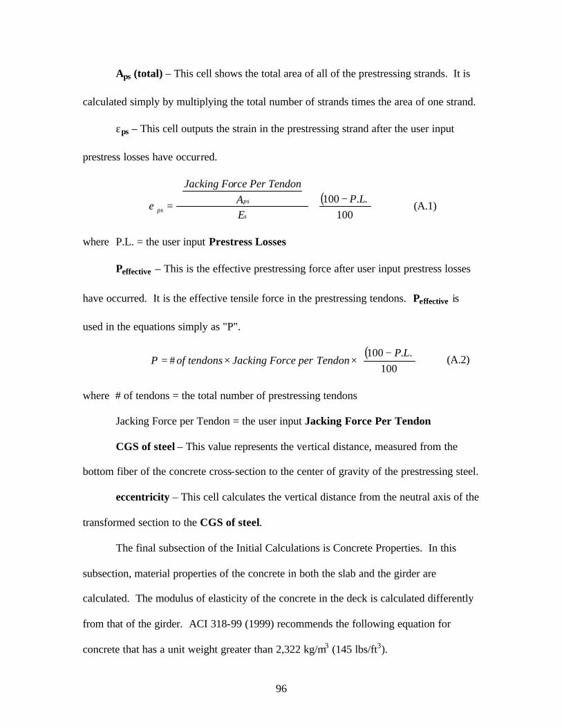
96

Aps (total) – This cell shows the total area of all of the prestressing strands. It is

calculated simply by multiplying the total number of strands times the area of one strand.

εps – This cell outputs the strain in the prestressing strand after the user input

prestress losses have occurred.

( )

−

⋅

=100

..100 LPEA

ndonrce Per TeJacking Fo

es

psps (A.1)

where P.L. = the user input Prestress Losses

Peffective – This is the effective prestressing force after user input prestress losses

have occurred. It is the effective tensile force in the prestressing tendons. Peffective is

used in the equations simply as "P".

( )

−

××=100

..100 #

LPTendonForce per Jackingof tendonsP (A.2)

where # of tendons = the total number of prestressing tendons

Jacking Force per Tendon = the user input Jacking Force Per Tendon

CGS of steel – This value represents the vertical distance, measured from the

bottom fiber of the concrete cross-section to the center of gravity of the prestressing steel.

eccentricity – This cell calculates the vertical distance from the neutral axis of the

transformed section to the CGS of steel.

The final subsection of the Initial Calculations is Concrete Properties. In this

subsection, material properties of the concrete in both the slab and the girder are

calculated. The modulus of elasticity of the concrete in the deck is calculated differently

from that of the girder. ACI 318-99 (1999) recommends the following equation for

concrete that has a unit weight greater than 2,322 kg/m3 (145 lbs/ft3).

97

1.5= deckfdeckE ccc '33(deck) )( γ (psi.) (A.3)

where Ec (deck) = modulus of elasticity of the concrete in the deck

Carrasquillo et al. (1981) recommend that for concretes with compressive

strengths exceeding 41.37 MPa (6,000 psi.) the following equation should be used to

compute the modulus of elasticity.

000,000,1'000,40)( +⋅=

girderfgirderE cc (psi.) (A.4)

where Ec (girder) = modulus of elasticity of the concrete in the girder

Equation A.3 is thought to overestimate the stiffness of higher strength concretes.

Cracked Beam assumes that the concrete used for the slab will have a compressive

strength less than 41.37 MPa (6,000 psi.) and that the girder will be fabricated using a

concrete with compressive strengths greater than this value. The values of n, k, and peak

strain were calculated using the same formulas for both the deck and slab. The equations

for each, which are shown below, were taken from Collins and Mitchell (1997). They

were used in the cracked analysis section to calculate concrete stresses. Only the

concrete compressive strengths varied in the computations of each.

n – This variable is a curve fitting factor that is found using the following

equation. 2500

'8.0

cfn += (psi.) (A.5)

Peak strain – This cell displays the peak strain, or the strain obtained when the

stress in the concrete reaches the maximum.

−⋅=

1'

'n

nEf

c

ccε (A.6)

where ε'c = the Peak Strain of the concrete

98

k – This is a factor that is used to increase the post peak decay in stress. It is

taken as 1.0 for (εc/ε 'c) < 1.0 and greater than 1.0 for (εc/ε 'c) > 1.0. k is calculated as

follows:

9000

'67.0

cfk += (psi.) (A.7)

Flexural Modulus – This cell outputs the tensile strength of the concrete in the

girder. It is estimated by the following equation.

(girder)cffr '5.7= (psi.) (A.8)

where ƒr is the Flexural Modulus of the concrete in the girder

Dead Load Weight – This is the total weight of the section per 0.305 m (1 ft.)

length of the girder. It takes into account the two individual concrete unit weights

entered for the slab and girder of the cross-section.

A.4 Uncracked Analysis

This section of Cracked Beam performs several static calculations assuming that

the girder is completely uncracked. Since cracking has not occurred, the assumption that

steel and concrete strains are equal at the same location remains valid. This allows for

the determination of steel stresses that would otherwise require a different and more in-

depth approach. Initially, four different moment calculations are required for the

Miscellaneous subsection.

Dead Load Moment – This cell provides the moment at the midspan of the girder

due to the dead load weight of the cross-section. This calculation, along with all other

calculations, is made with the assumption that the beam is simply supported. Equation

A.9 shows the calculation of Dead Load Moment.

99

( )

8 2LengthSpantLoad WeighDead

M DL⋅

= (A.9)

where MDL = Dead Load Moment

If a slab is included in the cross-section dimensions, then it is included in the

calculation of the dead load moment. If the user requires the moment due to the dead

load of the girder alone, then it is necessary to enter the cross-section without the slab.

Moment Due to Deck Only – This cell computes the portion of the dead load

moment that is caused by the weight of the girder deck only. If a deck is not included in

the analysis, then this cell value will be zero.

Decompression Moment – Due to prestressing, there will be a tensile force in the

tendons which causes a compressive stress in the concrete cross-section (usually greatest

at the bottom fiber). The Decompression Moment is the required moment applied at the

midspan of the girder to cause the bottom fiber of the girder to have no compressive

stresses. The following equation shows, in parenthesis, the calculation of the

decompression stress, which is multiplied by the section modulus to the bottom fiber.

The result is the Decompression Moment.

bbc

ZZ

ePAP

MomentionDecompress ⋅

⋅

+= (A.10)

where P = effective prestressing force in the tendons

Ac = non-transformed area of the cross-section

e = eccentricity of the prestressing force

Zb = transformed section modulus to the bottom fiber

Cracking Moment – This is the required moment applied at the midspan of the

girder to cause the concrete in the bottom fiber of the girder to crack. In order to crack

100

the concrete, the tensile stress in the bottom fiber of the cross-section must exceed the

flexural modulus of the concrete. Therefore, the flexural modulus of the concrete must

be added to the decompression stress before the moment can be determined. The

following equation shows, in parenthesis, the calculation of the tensile stress increase

required to cause cracking, which is multiplied by the section modulus to the bottom

fiber. The result is the Cracking Moment.

brbc

ZfZ

ePAP

omentCracking M ⋅

+⋅

+= (A.11)

where P = effective prestressing force in the tendons

Ac = non-transformed area of the cross-section

e = eccentricity of the prestressing force

Zb = transformed section modulus to the bottom fiber

ƒr = flexural modulus, or tensile strength, of the concrete

The next subsection of the Uncracked Calculations is the Dead Load Conditions.

In this subsection, the stresses and strains due to the dead load of the beam are calculated.

In addition, the steel stress in the bottom layer caused by dead load is also found.

Concrete stresses are determined by summing the stresses that are caused by prestressing

and the stress caused by the dead load weight of the section. Compressive stress is taken

as negative, while tension is positive. Equation A.12 shows the calculation of the bottom

fiber concrete stress due to dead load.

b

DL

b

DLb

ZM

ZeP

AP

fc

+⋅

−−= (A.12)

where fbDL = bottom fiber stress under dead load

MDL = Dead Load Moment from above

101

In order to find the concrete stress at the top fiber, Equation A.12 must be slightly

altered. The transformed section modulus to the bottom fiber, Zb, should be replaced

with the transformed section modulus to the top fiber. Once top and bottom fiber

concrete stresses are determined, the corresponding strains may be easily determined by

dividing the stresses by the moduli of elasticity of the respective concrete type.

The bottom tendon layer stress under dead load is equal to the stress caused by the

prestressing after losses have occurred. If a deck is being used for the analysis, then the

increase of steel stress caused by the weight of the deck is also added. This following

equation shows how the bottom layer tendon stress is calculated when a deck is not being

used.

σDL)( totalA

Pps

effective= (A.13)

where σDL= Bottom Tendon Layer Stress under dead load

Steel and Concrete Stress Calculator is the third subsection of the Uncracked

Analysis section. In this subsection, the user may enter a distributed load for which the

bottom tendon steel and concrete stresses will be calculated. After entering this load into

the Input a distributed load cell, it is added to the Dead Load Weight and the moment

caused by both the dead and distributed load is calculated. By using this Total Moment

in place of the Dead Load Moment in Equations A.12 and A.13, the steel and concrete

stresses can be determined for a distributed load. Once the top and bottom fiber concrete

stresses are known, then the strains can be calculated as before by dividing the stress by

the respective concrete modulus of elasticity.

The Steel and Concrete Stress Calculator provides the user another advantage. It

is possible to determine the distributed load that causes a given steel or concrete stress.

102

Calling the Tools/Goal Seek function of Excel, will open a window which requires the

following three input boxes — (1) "Set cell:" (2) "To value:" (3) "By changing cell:". In

the "Set cell:" input box, the user could enter the Bottom tendon layer stress cell from

Cracked Beam. It would then be possible to enter a desired Bottom tendon layer stress

in the Goal Seek box labeled "To value". Finally, the Enter a distributed load cell

should be inputted in the box labeled "By changing cell:". After inputting all three of the

Goal Seek boxes and pressing the enter key, the goal seek will begin. The result will give

the distributed load that causes the desired bottom tendon layer stress. This Goal Seek

can also be performed for the top and bottom fiber concrete stress cells. It is important to

note that all of the calculations performed in the Steel and Concrete Stress Calculator

subsection are not valid when the Total Moment exceeds the Cracking Moment

because this portion of the spreadsheet program is for uncracked analysis only.

The final subsection of the Uncracked Analysis section is Calculations for an

Input Moment. In this subsection, the user may enter a desired moment at which to

perform the analysis. Once the desired moment is entered, the top fiber concrete stress

and strain, bottom fiber concrete stress and strain, and bottom tendon layer stress, are

calculated based on the inputted moment. An analysis can be performed for a moment at

any section along the length of the girder. However, calculations in this subsection are

not valid when the Input Moment for the Analysis exceeds the Cracking Moment

since this portion of the program is for uncracked analysis only.

A.5 Cracked Analysis

The final section of Cracked Beam program provides a means to analyze a girder

that has previously been cracked. It is capable of determining the steel stresses, tensile

103

and compressive forces, the depth of the neutral axis, and the moment for any given top

fiber concrete compressive strain. Input Variables, Output, and Moment Finder are the

three subsections located within Cracked Beam. The user must enter two variables for

the Input Variables subsection.

c – This is the depth of the neutral axis. An assumed value should be entered.

εc – This cell requires the top fiber concrete compressive strain at which the

analysis will be run. A strain of 0.003 is recommended for ultimate moment analysis;

however, using the calculated peak strain from the Initial Calculations should also be

adequate. Figure A.3 shows the flow chart for the Cracked Analysis section of Cracked

Beam and the following paragraphs explain the steps in more detail.

Total tendon strain is calculated by summing the strain due to bending, the strain

due to the eccentricity of the prestressing force, and the strain caused by the initial

prestressing. If the top fiber of the girder has a certain compressive strain, then the

portion of the girder below the neutral axis will have a linear distribution of tensile strain.

This strain, which is the strain due to bending, is found easily by using similar triangles

formed with the user inputted top fiber strain and assumed depth to the neutral axis. It

may be a negative value, as the tendons can be located in the top flange of the girder.

The strain due to the eccentricity of the prestressing force refers to the amount of tensile

strain that must be added to the tendons in order for the strain distribution to be zero

along the entire depth of the section. Under prestressing, the girder would have a

negative curvature, or camber. In order to perform the cracked analysis, bending is

assumed to start from a section with zero curvature. Applying a moment to remove the

104

Start

Yes

Goal seek to find T - C = 0 bychanging “c”

Find the moment by summing the compressive forces × distance to the C.G.S.

No

Stop

Enter e c for the analysis

Assume “c”

Find the total strain in tendons

Find the stress in the tendons

Find the total tensile force in the tendons

Find the concrete strains in the compression zone

Find the concrete stresses at small intervals along the compression zone

Find the compressive forces in each section of the girder’s compression zone

Find the total compression force

Does tension equalcompression?

Figure A.3 Cracked Analysis Flow Chart

105

negative curvature would increase the strain in the prestressing tendons. This amount of

strain is known as the strain due to negative curvature. The third component of the total

strain is the strain due to prestressing. It is calculated in the Initial Calculations section

using Equation (A.1).

After the total strain in each tendon layer is known, Cracked Beam determines the

corresponding stresses. PCI (1999) recommends the following equations for 7-wire, low-

relaxation prestressing strands:

For 1,724 MPa (250 ksi.) strand:

εs ≤ 0.0076 fps = 28,500 (εs) (A.14)

−−=>

0064.004.0

250 :0076.0s

pss fε

ε (A.15)

For 1,862 MPa (270 ksi.) strand:

)(500,28 :0086.0 spss f εε ⋅=≤ (A.16)

−−=>

007.004.0

270 :0086.0s

pss fε

ε (A.17)

where εs = the total strain in the prestressing steel ƒps = the stress in the prestressing steel Once tendon stresses have been found, the total tensile force can easily be calculated by

multiplying the stress in a layer of tendons by the number of tendons in that layer.

The next step performed by Cracked Beam is the calculation of the concrete

strains in the compressive zone of the section. This calculation can be performed using

the relationship of similar triangles created by the assumed depth of the neutral axis and

the top fiber compressive strain in the concrete. Each section of the girder is treated

separately; both the area and centroid of the slab, top rectangle, top trapezoid, web,

106

bottom trapezoid, and bottom rectangle are calculated. The sections are shown in Figure

A.4.

Slab

Top Rectangle

Top Trapezoid

Web

Bottom Trapezoid

Bottom Rectangle

Figure A.4 Different Sections of the Girder

The number of strain calculations in a given section varies, depending on the

depth of the compression block. If the compression block only extends partially through

a section, then strain readings below the neutral axis will be zero.

Strains are taken at a number of sections so that an average stress can be

determined for each section of the girder. Within the concrete slab and the top rectangle,

strain is calculated at ten equally spaced increments. Only five increments are used to

calculate strains in both the top trapezoid and the web of the girder. As concrete strain

decreases, the stress distribution becomes more linear, so fewer increments can be used

without affecting the average stress of the section of the girder. Therefore, the bottom

trapezoid and bottom rectangle are only divided into three increments at which strain

107

calculations are made. The following equation shows the stress-strain relationship that

was recommended by Collins and Mitchell 1997) and also used in this program.

( )( )

( )

+−

⋅⋅= nk

cc

cc

cc

n

nff

'1''

εεε

ε (psi.) (A.18)

where ε’c = the Peak Strain of the concrete (see Equation 6.6) εc = the strain in the concrete n = the curve fitting factor (see Equation 6.5) k = factor to increase post peak decay (see Equation 6.7) ƒ'c = the concrete strength (could be the slab or the girder) Cracked Beam makes a summation of all of the stress values in one section of the

girder divided by the number of times stress was calculated in that particular section.

This gives the average compressive stress for that section. Multiplying this average stress

of the section by the area of the section gives the compressive force in that section.

Cracked Beam then multiplies these compressive forces by the distance from the centroid

of the section to the center of gravity of the steel. After summing all of these moments,

the total moment of the section is displayed in the Output subsection. It is important to

note that if the "T – C" cell does not equal to zero, then the moment is incorrect because

the force equilibrium has not been satisfied.

In order to satisfy the force equilibrium, it is necessary to find the depth of the

neutral axis such that the total tensile and compressive forces are equal. The user must

use the Tools/Goal Seek function of Microsoft Excel. This will open the Goal Seek

window which requires the following three input boxes: (1) "Set cell:" (2) "To value:"

(3) "By changing cell:". In the "Set cell:" input box, the user should enter the "T – C"

cell from Cracked Beam. Zero should be entered for the Goal Seek box labeled "To

value:", and the Cracked Beam cell "c" should be entered for the box labeled "By

108

changing cell:". After entering all three of the Goal Seek boxes and pressing the enter

key, the goal seek will begin. The result will provide a "c" value for a given top fiber

strain, where the total tensile force equals the total compressive force. In addition, the

corresponding total moment will be correct, as the force equilibrium has been satisfied.

In some instances when the assumed value of the neutral axis is greater than the actual

value, the Goal Seek function may not be able to find a solution. In the unlikely event

that this happens, it is necessary to re-enter the assumed value of "c". A smaller value,

but not zero, should be entered and the process then repeated.

If the user desires to perform an analysis at a specific moment, lower than the

ultimate moment, it is necessary to follow an iterative process to most efficiently

determine the top fiber strain at this desired moment. Rather than using trial and error

with different strain values, the subsection Moment Finder can be used to quickly

interpolate the compressive strain that corresponds to a desired moment. The user begins

by entering the moment at which an analysis will be performed in the Desired Moment

cell. In the table below the Desired Moment cell, the user enters the strain at ultimate in

the left column and the corresponding moment in the right column. Next, the user must

use the Goal Seek function at two or more lower strain values. These strains, and their

corresponding moments should also be entered in the same table. The graph, found in the

Moment Finder subsection, will then plot the line formed by the strain and moment

coordinates. In addition, the graph also plots a line representing the desired moment.

The strain value, which is shown on the horizontal axis of the graph, where the two lines

intersect represents the strain at which the desired moment occurs. Performing a Goal

Seek, as described above, with this strain should result in a moment that is very close to

109

the desired moment. A few more trial and error strain iterations may be needed to

exactly pinpoint the desired moment. If the two lines on the graph do not intercept, then

the trial strains are not low enough. Two lower strains should be chosen and then the

process should be repeated.

110

APPENDIX B

Samples of Input and Output of Cracked Beam Program

111

112

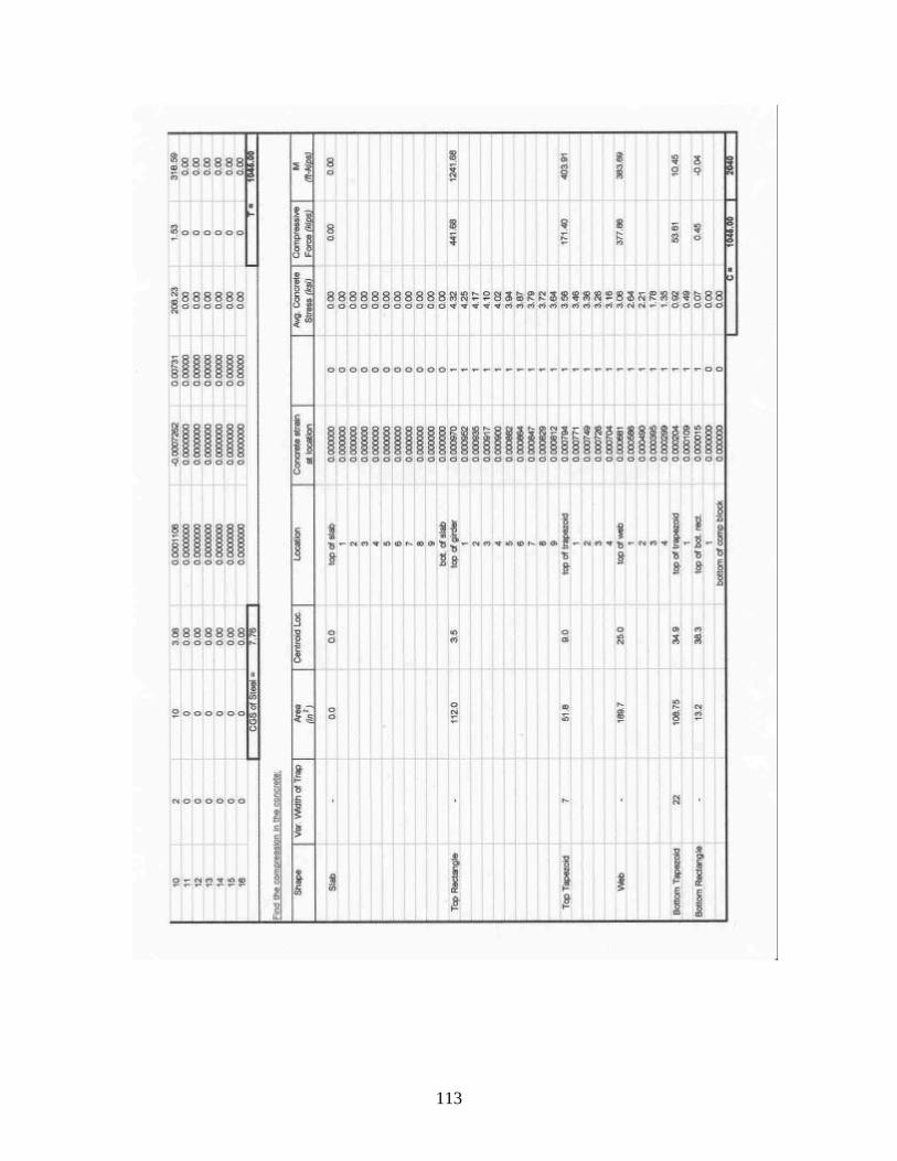
113

114

APPENDIX C

Response 2000© Program Procedure

115

RESPONSE 2000© PROCEDURE C.1 Introduction

Response 2000 is a non- linear concrete sectional analysis program developed by

Bentz (2000). The computer program consists of over 150,000 lines of C++. In this

program, the basic assumptions of prestressed concrete are defined along with the fact

that there is no transverse clamping stress across the depth of the beam. In addition to

Response 2000, Bentz also developed Membrane-2000, Triax-2000, and Shell-2000.

These programs analyze their respective namesakes and are included in the entire user

manual, which can be found online at www.ecf.utoronto.ca/~bentz/r2k.htm. Appendix D

gives selected sections from the entire user manual that will be referenced herein. This

appendix will discuss the steps needed to develop and analyze a prestressed concrete

bridge girder using Response 2000 (version 1.0.0). Any further questions or inquiries

about any of these programs can be directed to Evan Bentz at bentz@ecf.utoronto.ca.

C.2 File Setup and Beam Description

To begin file setup and beam description, go to "Options | Preferences" where the

units can be changed between SI Metric, US Customary, or kg/cm Metric. From this

point a cross-section needs to be entered. Go to "Define | Quick Define" to input the

appropriate material properties and section properties. The first step asks for a title and

the material properties. These material properties can be altered at a later time if

necessary. The second step of the quick define is the concrete cross-sectional

dimensions. There are general shapes that are already pre-dimensioned such as PCI-

Double-T and AASHTO girders. Other shapes that are listed can be chosen and then

dimensioned using the appropriate input boxes located to the right of the screen. If there

116

is not a section that directly correlates to the section to be analyzed, a similar section can

be chosen and then modified later. These modifications will be discussed later in this

appendix. The third of four steps is the reinforcement designation page. This page

allows top and bottom non-prestressed reinforcement to be selected by area or

designation. A table of the available designations is located in Table 2-4 in Appendix D.

The fourth and final step of the quick define menu is to input stirrups and prestressed

tendons. Like the previous step, the stirrups can be selected in one of two ways. The

tendons are inputted by number and prestressing strain in the strands. Again, the

properties listed in steps 3 and 4 can be modified later if necessary. To finish the "quick

define" section, click "Finish".

After clicking "Finish", the cross-section and geometric properties will be

displayed. From this screen many of the properties can be modified or added. For

example, if the cross section needs to be modified, simply double click within the cross-

section area and the "define concrete cross section" screen will appear. This applies to

reinforcement (prestressed, non-prestressed, and stirrups), loading, crack spacing,

material properties and even the title block. Another way to access the menu for a

specific item is to go to "Define | _____". In this blank, the menu that needs to be

modified can be chosen. Again, using the same example as before, if the cross section

needs to be modified, go to "Define | Concrete Section". This menu will then have three

tabs that can be chosen to develop the appropriate cross section. The first tab contains

basic shapes that the user can insert values for pre-defined dimensions and the cross-

section will be produced. The second tab is used if an uncommon section or a

modification of a standard shape needs to be created. Widths of the cross section can be

117

inputted at certain heights of the section. After each width and height is inputted, the

button marked "Modify" or "Add" should be clicked to make the change or addition to

the section. The third tab is marked "standard shapes". This tab contains cross sections

of standard sections. In this section an AASHTO beam or PCI beam can be chosen, for

example. There is also a box that can be checked to add a slab with dimensions that the

user can specify.

C.3 Material Properties

The next modifications and/or additions that probably need to be made are

associated with the material properties of the concrete and steel. Like the concrete

section, these properties can be accessed by double clicking on the text describing the

material, the graph describing the behavior of the material, or through the "Define |

Material Properties" menu. Once into the "Material Properties" menu, there are three

choices: Concrete, Non-Prestressed Reinforcement, and Prestressed Reinforcement.

These three sub-menus will now be described in more detail. Further discussion of these

menus is contained in the full user manual located in Appendix D. This will be referred

to often for examples and tables.

C.3.1 Material Properties: Concrete

The concrete sub-menu of the material properties page can be accessed by

clicking on the "detailed f′c" button. In this menu, there are eight fields that can be

entered. The first field is the concrete compressive strength. In this box the design

compressive strength of the concrete should be entered. From this number the second

field will be calculated. This option is used when the word "auto" appears in the field

box. This "auto" refers to the automatic calculation of the tension strength. As

118

mentioned in Table 2-1 of Appendix D, this tensile strength should be used as the ACI

shear cracking stress, but can be changed to a user-defined number if the user should

decide to do so. The next field is the peak strain, which is also calculated automatically

based on the Base (stress-strain) Curve included in the program, but can be changed to a

different value. The options, in past versions of Response 2000, for Base Curve were

either parabolic or Popovics / Thorenfeldt / Collins, but in v. 1.0.0, the only option is the

latter. This option is the modeling of the compressive stress-strain curve of the concrete.

The peak strain for a Popovics model can be found in Collins and Mitchell (1997) as

ε1

''

−=

nn

Ef

c

cce (C.1)

where ε’c = peak strain f‘c = compressive strength (psi) Ec = Modulus of Elasticity of the concrete (psi) n = 0.8 + f‘c / 2500 (psi) This is the equation that is used in the Response program to find the automatic peak strain

value. It is a part of the Popovics equation that is also used in the program. The key part

of this equation is the calculation of Ec. As cited in Collins and Mitchell (1997),

Carrasquillo, Nilson, and Slate (1981) proposed that for concrete compressive strengths

over 41.4 MPa (6,000 psi) the equation for Ec should be

000,000,1'000,40 += cfEc (C.2)

as opposed to the ACI equations for Ec. Using this equation results in a smaller value for

the modulus of elasticity which, when using a composite structure, gives a larger steel to

concrete modular ratio. Also, it should be noted that changing the peak stress manually

will affect the value given for the modulus of elasticity of the concrete. To check the

initial stiffness of either the concrete or the steel, right click on the appropriate stress-

119

strain graph on the cross-section screen. This will give the user a menu where "Initial

Stiffness" will be a choice. Click on that option and the Modulus of that material will be

shown.

Following the peak strain is the aggregate size. The default value of 19 mm (0.75

in.) is given in most files. After the aggregate size is the tension stiffness factor. This

factor is related to the tension stiffening field number eight, but can be manually changed

to a value less than unity. The only option that Response 2000 version 1.0.0 will

acknowledge for the tension stiffening is the Bentz 1999 option, which is associated with

a default value of 1.0 for the tension stiffness factor. This is also the case with field

numbers six and seven. The final field to be entered in is the Compression Softening box,

which can only be chosen as Vecchio / Collins 1986. As mentioned previously, Table 2-

1 in Appendix D gives further discussion about the different options on this sub-menu

and other menus within the material properties menu.

When modeling a girder with a deck slab attached, two different concrete

compressive strengths would be needed. To account for this difference, two separate

concrete types should be used. While in the concrete menu, change the name cell in the

type list to reflect what is being modeled, such as slab. Then make the appropriate

changes to the properties and click "Add". This will add the new concrete type. After

creating a new concrete type, the user must return to the "Define | Concrete Section"

menu to apply this type to the slab. Once in the menu, click on the slab in the drawing of

the girder and slab, and a pop-up window will appear. In this window will be the choices

for the types of concrete. Choose the appropriate concrete type and click "OK". This

difference will be shown on the cross-section screen to the left of the cross-section.

120

C.3.2 Material Properties: Non-Prestressed Reinforcement

Below the Concrete section of the material properties page is the Non-Prestressed

Reinforcement section. To access this sub-menu simply click on the "detailed fy" button

located on the right side of the menu. There are six fields that can be entered on this

menu and most of them are standard values. Fields one and two are values of which are

usually considered to be constant for non-prestressed reinforcement. If these values need

to be changed from the existing values, simply click in the field, delete the existing value,

type in the appropriate number, and then click on the modify button on the left side of the

screen. This will modify the steel that you have inserted in your section. If there is more

than one type of steel, and/or multiple layers of non-prestressed reinforcement, then there

will be more than one name in the type list. When the user needs to modify an existing

layer or type, simply click on the appropriate name (which the user can assign) and then

input the values and press "modify". If a new layer or type needs to be added, put the

cursor in the name box and erase the existing name and type a new one and then click the

"Add" button. This will give the user a new layer or type of steel. This process is typical

with all the sub-menus in this program. The fields within this sub-menu are best

explained in Table 2-1 of Appendix D. The third and final sub-menu of the Material

Properties page, Prestressed Reinforcement, will now be discussed.

C.3.3 Material Properties: Prestressed Reinforcement

As with the previous two sections, this menu can be accessed by clicking on the

"Detailed fpu" button on the right side of the screen. In this menu, the values for each

field are also typical values for the type of prestressing steel that is listed in field seven.

In field seven, three different options can be chosen: Custom Type, 1,860 MPa (270 ksi)

121

Low-Relaxation, and 1,860 MPa (270 ksi) Stress-Relieved. If either of the two latter

options are chosen, then fields one through six will be automatically chosen for the user

based on values that are associated with that type of strand. If the first option, Custom

Type, is chosen then the values will be based solely on the user’s input. The first three

input fields are constants that are used in the Ramberg-Osgood equation to calculate the

steel stresses. It should be noted that using the Ramberg-Osgood equation gives steel

stresses that are smaller in magnitude than using the stress-strain curve equations found

in PCI Handbook (1999). Further information regarding the Ramberg-Osgood method

can be found in Collins and Mitchell (1997). Table 2-1 in Appendix D further explains

the details behind each of the fields in this menu.

After the user has modified these three sub-menus, the topic of geometry of the

non-prestressed and prestressed reinforcing steel will be addressed.

C.4 Steel Geometry and Layout

In the "Define | Quick Define" menu, steps three and four asked for preliminary

inputs for the reinforcement details. In the following section, more detailed information

can be added to the information that has already been entered.

C.4.1 Steel Geometry and Layout: Transverse Reinforcement

The first menu is "Define | Transverse Reinforcement". This menu contains six

fields, which are straightforward. The small check box next to "Selection Type" is used

if the user would like to select the bar type by its area. If this box is not selected, then the

steel designation can be used to choose the appropriate steel. This check box is typical

within these three steel menus. The appropriate steel designations are listed in Table 2-4

in Appendix D. This table contains an extensive listing of bar and strand designations,

122

but if the user would like to add to this list of bar designations, there are directions listed

in Section 5-8 of Appendix D that show how new bar designations can be added to the

database. This menu operates like the previous and following menus in that there may be

more than one type of stirrup and this can be added or modified using the left side of the

screen.

C.4.2 Steel Geometry and Layout: Longitudinal Steel

The next section in the steel defining step is the "Define | Longitudinal Steel"

menu. This menu contains three tabs located across the top of the window. The first tab

will be discussed herein. Tabs two and three were not used in this NCDOT project and

are explained in Section 2-5 of Appendix D. Individual layers of longitudinal steel can

be added using the first tab. Within this sub-menu, there are four fields to be inputted not

including the Selection Type check box. This sub-menu is easily inputted and any

additional information needed can be located in Section 2-5 of Appendix D.

C.4.3 Steel Geometry and Layout: Tendons

The next and final sub-menu dealing with the steel geometry and layout is the

"Define | Tendons" sub-menu. This menu contains more detailed fields to be inputted

and will be discussed in a little more detail. First, most prestressed members will contain

more than one layer of prestressing, and therefore additional layers need to be added to

the Layer List. After the appropriate number of layers has been added, each individual

layer can be modified. Click on the layer that needs to be changed and the fields on the

right of the screen will display the values that have been inputted so far for this layer.

The first field is the number of tendons that will be in this layer. The horizontal position

of these tendons will not be user controlled and therefore there will not be any input areas

123

for this dimension. After the number of tendons is entered, the area or designation can be

inputted. The third field is the prestrain value. This value is defined as the jacking force

of an individual strand divided by the area of that strand and then that quotient is divided

by the modulus of elasticity of steel. This should give a number with at least two decimal

spaces before the first non-zero number (such as 0.00711). This number will be the

initial prestrain value. To account for any losses that may occur in the strands, Response

2000 version 1.0.0 contains an option listed as "Loads | Time Dependent Effect" that will

model the appropriate losses over a specified life of the member. To activate this option,

simply go to "Loads | Time Dependent Effect" and click the "Consider Time Dependent

Effects" check box and enter the age for analysis and sustained moment. Any further

information regarding this option can be found in Section 3-5 of Appendix D. To input

the value, the user should multiply the actual value by 1,000 to get the appropriate units

of milli-strain.

The next field is the distance from the bottom of the concrete section. This value

will depend on the location of the specific layer of steel. Following this value will be the

slope of tendon field. This value is how much slope the layer of tendons have at the

section that is being analyzed. Most sections are analyzed at midspan, and would have

zero slope, but if the section being analyzed is not where tendons are straight, then the

slope of the tendon, in percentage, should be entered in this box. Since this is a dual

section analysis the computer analyzes the cross section that is inputted and then a section

directly next to the cross section to determine the data that is presented in the results. The

last field that is in this window is the Tendon Type. This value was entered in the “Quick

Define” menu at the beginning of the file. It should show either Low Relax or Psteel 1.

124

Psteel 1 is the designation given to stress relieved strands. After checking to make sure

this value matches the value entered in the initial menu, click "Modify", if the user made

changes, or "Add" if the user added a new layer of steel. Once this is accomplished

simply click "OK" and the tendons will be shown on the cross section of the member.

If any of the values inputted in the steel defining steps needs to be revised, the

user can double-click on the description of the steel that needs changing. For example, if

(2) 0.153 in.2 tendons were inputted, there should be wording describ ing this and simply

double click on that wording and the appropriate screen will appear for making any

necessary changes.

C.5 Loads

Once the concrete and steel properties are defined and the cross-section is

developed, the next step is to input the loads. In this program the loading is done as a

proportion and not as exact values. To access the loading screen click "Loads | Loads"

and there will be a window that has six input fields. The three left fields are constant

loading values that are used for a single load analysis or a starting load level. In the

analysis of the NCDOT test girders covered in this report, the constant loading values

were not used. Loads were inputted only in the "increment" fields. The actual

magnitudes of the loads are not necessary, only the proportion relative to each other. The

general equation for the ratio is simply,

VM

ratio = (C-3)

where M is the equation for the moment at the section of the beam being analyzed and V

is the corresponding equation fo r shear at this section. Two examples of the calculation

necessary to produce the ratio is shown below.

125

The first example will detail the load setup used to test the NCDOT girders and

the second example will be a distributed load, which would be the common load case for

design. If there is a single point load acting at the midspan of the beam and the midspan

is the section being analyzed, then the equations for the moment and the shear are

4

PLM = (C-4)

2P

V = (C-5)

where P = point load applied (lbs.)

L = span length of the beam (ft.)

Therefore, the ratio VM

would give a result of 2L

. This value would be inputted into the

moment box and a value of 1 can be inputted into the shear box. If a distributed load is

applied to the beam and the beam is being analyzed at midspan, then the equations used

are

8

2LM

w= (C-6)

2L

Vw

= (C-7)

where w = distributed load over the beam (lbs./ft.) L = span length of the beam (ft.)

Inserting these equations into Equation (C-3) results in an equation of 4L

. This value

would be inputted into the moment box with a 1 inputted for shear. Once these loads are

inputted, the program is ready to run.

The following sub-menu of the "Load" menu is "Time Dependent Effects". By

using this option, Response 2000 will account for prestress losses at the specified age of

126

the girder. This process was detailed in Section C.4.3 previously and is explained further

in Section 3-5 of Appendix D. After this sub-menu, there are three other options, two of

which are not covered here but are discussed in detail in Section 3-5 of Appendix D.

These options can allow for more details to be inputted on the section being analyzed. In

the analysis of the NCDOT girders, these options were not explored. The third option is

labeled as "Full Member Properties" and was used in this project.

This menu allows for input that will enable the program to analyze the beam as a

full member and show the crack pattern over the full length. The first input cell is the

length subjected to shear. For this project, this length was simply half the span length of

the girder because a point load was applied at the midspan. If, for example, two point

loads were used, each at equal distances from the midspan, then the length subjected to

shear would be the distance from the support to the point load. This type of loading

would also result in a constant moment region between the two point loads. The second

input cell accounts for this constant moment. For this example, this cell would be the

distance from one of the point loads to the midspan, assuming these point loads are

symmetrical. Below the two input cells are three options describing how the beam is

loaded. For this project, the first option was chosen, point loads. As these options are

chosen the picture to the right of the screen shows how the moment diagram would look.

Following the loading options is a cell asking for what percentage of the moment the left

side of the beam has as compared to the right side. For a simply supported beam, such as

the one analyzed in this project, this value would be zero. If a beam was a multiple-span

beam that was able to carry a moment at the left side, then this value could be a number

other than zero. After these cells have been entered, there are two more options to

127

choose. The first is the left side properties and the second is the right side properties. For

both of these the first option was used to model this girder. These, as the previous

loading options, are dependent on how the load is applied and the beam is arranged.

Once these values are inputted the program is ready to run.

C.6 Analysis Options

After the input for the section and the loads have been entered, the section is

ready to be analyzed. In the "Solve" menu, there are ten sub-menus that can be chosen,

each dealing with a different type of analysis. The only two analysis options that were

used in the project were the "Sectional Response" and the "Member Response" options.

The "Sectional Response" option calculates the single load, if one is inputted, and then

applies the incremental load until failure. The "Member Response" option shows the full

member properties and analyzes the entire beam. The other options, excluding the "One

Load" option, are strain state analyses and are discussed further in Section 4-2 of

Appendix D.

C.6.1 Analysis Options: Sectional Response

When "Sectional Response" is selected from the "Solve" menu, the screen will

show two graphs on the left side of the screen and nine pictures/charts on the right.

These graphs will progress through the incremental load steps and show the user how the

section is reacting to the loads. Once the analysis is complete (15 seconds, or more if the

section is really complex) the ultimate moment and curvature will be displayed on the

bottom left graph marked M-Phi. This moment is the total moment capacity of the

section. In order to find the necessary applied load to cause this moment, the dead load

moment of the member must be subtracted from the total moment and then the resulting

128

moment can be used to find the applied load. The stress and strain properties of the

section at this load are shown in nine graphs on the right-hand side. Among these graphs

are the cross section, which shows what part of the concrete has cracked, and the crack

diagram that shows the location and widths of these cracks. The other seven graphs show

stresses and strains of the steel and concrete. If these properties are desired for another

load level, such as at cracking, the user can click on the M-Phi graph to change the load

level. Once on the M-Phi graph, use the "Page Up" and "Page Down" but tons to scroll

through the load levels.

If another type of graph is desired it can be accessed a number of different ways.

The "View | _____" menu has different options that can be chosen depending on the

graphs requested. The first sub-menu under "View" is the "Cross Section". This simply

shows the cross section as seen in previous screens before analysis. Following "Cross

Section" is "1 Cross Section Plot", which shows a window that is the size of the screen,

where any of the 24 graphs can be viewed. While in this window, the load level can be

scrolled by clicking on the M-Phi graph as before and using the "Page Up" and "Page

Down" keys, or by going to the "View | _____" menu and selecting "Next Load Stage" or

"Previous Load Stage". The next option is the "9 Cross Section Plots". This window is

the same window that appears when the analysis was initially completed and has the

capabilities of showing all the graphs possible, nine at a time. While in this window, or

in any window containing a graph, the graph can be right clicked on and a menu of

options will appear. Within this menu are options dealing with the visual effects of the

graph and the data of the graph. The "View Data" option is helpful when trying to find a

specific value at a specified depth of the section. The option called "Load Deformation

129

Plot" in the "View" menu is an option that is aimed at giving information relating the load

and other variables of the results. This option is detailed in Section 4-4 of Appendix D.

This option is beneficial when reporting the results in graphical form because it can show

the behavior of the beam with sub-menus pasted onto the graph.

C.6.2 Analysis Options: Member Response

The second analysis option used in this project is the "Member Response" option.

When this option is chosen the same screen comes up as when the "Sectional Response"

was chosen. This screen does not contain information that is needed when doing a full

member response analysis. After the analysis is complete (30 seconds) another screen

will appear that will show half of the beam, four graphs below, and two to the left of the

screen. The bottom left graph shows the load-displacement curve of the beam. The P

value that is listed is the point load for half the beam and should be doubled if an applied

point load is desired. The beam figure shows the crack pattern of the girder at the

associated load level. Below the beam are four graphs that show the reaction of the beam

under loading arrangement. As before, the user can right click on the graphs and pull up

a menu that allows the user to change the visual properties as well as view the data in a

table form.

The top left graph shows the curvature along the length of the beam. This is

helpful in determining the displacement of the specimen, which is shown in the graph at

the bottom left. The top right graph shows the shear strain along the length of the beam

while the bottom right graph shows the shear force versus displacement. As mentioned

previously, clicking on the P-∆ graph and using the "Page-Up" and "Page-Down" keys

130

can change the load level. Individual graphs can be shown, as before, by going to the

"View" menu and selecting the appropriate option.

This discussion gave a brief overview of the steps taken to model a prestressed

concrete girder such as the one tested for this project and some of the capabilities of the

program. Response 2000 has many other capabilities and the full user manual should be

consulted to learn even more about this program.

131

APPENDIX D

Selected Sections of the Total Response-2000 User’s Manual (Bentz, 2000)

(Shown with permission of Evan Bentz)

132

Quick Start: Response-2000

Response-2000 is perhaps the most immediately useful of the four programs explained in this manual. It allows analysis of beams and columns subjected to arbitrary combinations of axial load, moment and shear. It also includes a method to integrate the sectional behaviour for simple prismatic beam-segments. The assumptions implicit in the program are that plane sections remain plane, and that there is no transverse

clamping stress across the depth of the beam. For sections of a beam or column a reasonable distance away from a support or point load, these are excellent assumptions. These are the same locations in beams that are usually the critical locations for brittle shear failures.

Unlike the other programs, Response-2000 doesn’t have a default cross section entered into it. This isn’t a real problem, however, as one can be made quickly. For this example, an 80 foot span prestressed concrete bridge girder and slab will be analysed.

First, as this example is presented with US customary units rather than the default SI metric, select it from the “Options | Preferences” dialog box. To select US units as a default each time the program begins, see section 5-11 of this manual.

Secondly, go to the “Define | Quick Define” dialog box. This is a “wizard” that allows a section to be created quite quickly, usually within 30 seconds. Each of the four programs in this manual has such a wizard to make new files quickly.

The first page of the dialog box asks for a title and material properties. After entering a title, say, “Test Section” with the reader’s initials for the “Analysis by” box, the material properties may be selected. For this example, the 5000 psi concrete, 60 ksi steel and 270 ksi strands are fine, so select the “Next” button.

The second page of the wizard asks for the concrete cross section. At the top of the list are simple sections such as rectangles and circles. In the middle of the list are more exotic shapes such as columns with interlocking hoops, and hollow columns. At the bottom are the “standard shapes” such as AASHTO girders. As this is what is needed here, scroll down near the bottom of the list and select “Standard Shapes AASHTO”. Press tab (or click with the mouse) to the right side to select the type of section. Pressing any key will pop up a selection box to select a section from the currently defined listings. Select the AASHTO Type IV girder and press “ok”. For the next input field, enter zero, as there will be no “haunch” on this section (i.e., no extra concrete between the top of the precast beam and the bottom of the slab.) Select a slab depth of 8 inches, and a slab width of 80 inches, and select Next to go to the next page of the wizard.

133

The third page allows selection of the longitudinal reinforcement for the section. The top half defines bars in the slab for this standard cross section case and the bottom defines non-prestressed steel in the bottom of the cross section. Leave the default of 20 #4 bars for the top, but remove the 3 #8 bars for the bottom by entering “0” for the number of bars in the bottom half of the screen. Press the Next button again to go to the last page of the quick menu.

The last page allows selection of the stirrups as well as the strands. Select “open stirrup” from the list of stirrup types. The default bar type of #4 is reasonable. Select a spacing of 16 inches. Switch the clear cover to 2 inches from the default value, which is actually 40 mm converted to inches. Finally, enter 30 for the number of strands. The prestrain listed as 6.5 represents a jacking stress of 70% of ultimate, and is therefore reasonable. Select the “Finish” button to complete the definition of the section. Automatic Cross Section

Response-2000 will automatically create the cross section as shown below similar to the one from Membrane-2000. As with the other programs, changing the geometry is achieved either through the use of the “define” menu or by double clicking on the drawing itself. For example, to change the stirrup spacing, double click on the text in the drawing where it says “#4 @ 16.00 in.” Like all the programs, this page is meant to include all the information needed to repeat the analysis or document it in the course of a design.

Test Section

ECB 1999/8/23

All dimensions in inchesClear cover to transverse reinforcment = 2.00 in

Inertia (in4)

Area (in2)

yt (in)

yb (in)

St (in3)

Sb (in3)

1423.8

649082.1

22.2

39.8

29241.2

16307.6

1480.4

694653.1

22.6

39.4

30725.3

17634.6

Gross Conc. Trans (n=7.58)

Geometric Properties

Crack Spacing

Loading (N,M,V + dN,dM,dV)

2 x dist + 0.1 db /ρ

0.0 , 0.0 , 0.0 + 0.0 , 1.0 , 0.0

26.0

80.0

8.062.0

2 layers of 10 - #4

#4 @ 16.00 in

30 - S.5∆εp = 6.50 ms

Concrete

εc' = 2.02 ms

fc' = 5000 psi

a = 0.75 inft = 269 psi (auto)

Rebar

εs = 100.0 ms

fu = 90 ksi

fy= 60

P-Steel

εp = 43.0 ms

fpu = 270 ksi

Low Relax

134

Analysis without Shear

The default type of analysis for a new section is a simple flexural analysis with no axial load. To start it, select “Solve | Sectiona l Response” from the menu. The analysis should take perhaps two seconds to complete. The control plot will show up along with 9 plots as in Membrane-2000. In the case of Response-2000, the plots all represent the given variable plotted over the depth of the section for the load stage indicated by the control plot. Click on the “Auto Range” button on the top left of the screen below the menu to automate the scale of the plots, and click anywhere on the control plot. All the plots will automatically change depending on the new location on the control plot. Note that the loading is listed in the bottom bar of the program window. The crack diagram shows predicted crack widths in inches as well as an estimate of the pattern of cracking. Analysis with Shear

A more involved analysis type, one that Response-2000 excels at, is the prediction of sectional behaviour including the effects of shear. For a beam like this, it may be decided to perform an analysis at a location ‘d’ from the end of the beam. At a uniformly applied load of 3.0 kips/ft, the moment and shear at this location are about 435 kip.ft and 109 kips respectively. These loads are entered into the Response-2000 “Loads | Loads” menu option. This menu has a left and right side, where the left is for initial loads and the right is for any increment in load beyond that level. Leave the left values as zero and set the right side value for moment to 435 kip.ft and shear value to 109 kips. Note that the actual numbers here don’t matter, only the ratios and signs. After clicking the “ok” button, select “Solve | Sectional Response” to start the analysis. The analysis should take about 10 seconds to reach the peak load, and then about 20 more seconds to determine the post-peak ductility for the section. The following 9-plot screen will show up. These plots represent the state of the beam at failure, as shown by the location of the crosshairs on the control plots. Each plot is drawn with respect to the depth of the section. For example, the top centre plot shows the longitudinal strain versus depth for the section showing the basic assumption that plane sections remain plane. Briefly, the cross section in the top left is drawn darker in regions where it is predicted not to have cracked. In this case, only the web of the beam is predicted to be cracked at the shown failure load. The top right shows the variation in transverse strain over the depth, with a maximum of 7 mm/m near the top of the web. The crack diagram shows the predicted angle and width of cracks in inches. The shear stress plot shows that the shear is not uniformly distributed over the depth of the section, though is fairly constant in the web at about 630 psi.

135

The bottom left plot of the 9 plots shows the principal compressive stress values. The line at the left of the plot is the maximum allowed stress versus depth and the right line shows the applied stress. Note the shear has applied an additional diagonal compression in the web on top of the expected concrete stress profile from the prestressing force. The two lines on this plot are about to touch at the top of the web indicating that this section is about to fail by crushing of the web. The two control plots show that the “V-Gxy” curve, that is, the shear-shear strain plot, is descending with increasing shear strain, whereas the lower moment curvature plot is unloading along its loading curve. This indicates that the section is predicted to fail in shear. The maximum predicted shear capacity of the section is 249.4 kips. By scaling this from the loading, it is predicted that the beam would fail in shear at this location if the applied load were to increase to a level of 7.0 kips/foot. Member Response

Response-2000 will calculate the full member behaviour for a prismatic section as well. To get a prediction of the behaviour of this 80-foot beam, such an analysis will be performed with the beam subjected to a uniformly distributed load. First select the “Load | Full Member Properties” menu option. Select the “length subjected to shear” at the top as 480 inches. (The analysis is done from one end to the mid-span of the beam.) Also select in the top options a uniform distributed load rather than a constant shear analysis.

136

This is the second option in the top list of three buttons. Click “ok” and select the “Solve | Member Response” option.

This analysis will calculate an entire Moment-Shear interaction diagram and determine the load-deflection properties and crack diagram for the entire 40 foot half span of the beam. The analysis on an inexpensive 400 MHz Pentium II takes about 60 seconds to complete. As the analysis continues, the growing M-V interaction diagram will be shown on the control plots. Periodically, the 9 plots will also update showing the sectional behaviour at the location of the crosshairs on the control plots. The transition from flexural failures under positive moment at the right of the interaction diagram gives way to shear failures at the top of the interaction diagram and then back to flexural failures under negative moment at the left side. By clicking on the little squares on the plot, any of the integration points may be examined so see how the beam is behaving at that load combination.

When the analysis is complete, the screen will change to the deflection page as shown below. The top diagram is the predicted crack pattern at failure for the entire 40 foot section of beam. The bearing support plate at the left bottom can be seen, and the right side represents the midspan of the beam. Estimated crack widths are shown in inches. In the top control plot at the left is the M-V interaction diagram as well as the applied loading for this beam shown in red. For a uniformly distributed load, such as this, the majority of the loading is a parabola, with the load cut down to zero near the support due to non-sectional load resistance methods. The explanation for the shape of

137

this load diagram can be found in reference 2. It can be seen from the interaction diagram that the loading envelope is touching the strength envelope almost simultaneously at the right side bottom (flexure in positive moment at midspan), as well as at the top (shear near support). Indeed, the midspan cracks are predicted to be almost 1 inch wide, and there is substantial shear cracking (0.147 inch cracks) near the support.

The bottom control plot shows the predicted load-deflection relationship for the beam (pushover analysis results for column analyses). The final behaviour is predicted to be fairly ductile, with a 22.9 inch deflection at a failure load of 7.13 kips/foot. Assuming that the load capacity is acceptable, this would seem to be a fairly efficient design in terms of shear versus flexural capacity; more stirrups would not be needed, as the beam would fail in flexure first. A lower amount of stirrups would subject the beam to a potentially brittle shear failure, however. In a design like this, it may be wise to err on the conservative side of shear design, however, and include a little bit more shear reinforcement than what has been provided. Of course Response-2000 allows any such option to be quickly checked by changing the spacing of the stirrups, and quickly rerunning the analysis.

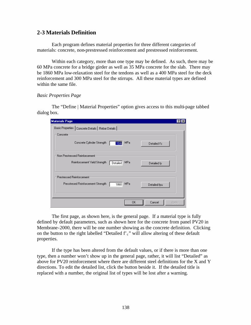
138

2-3 Materials Definition

Each program defines material properties for three different categories of materials: concrete, non-prestressed reinforcement and prestressed reinforcement.

Within each category, more than one type may be defined. As such, there may be 60 MPa concrete for a bridge girder as well as 35 MPa concrete for the slab. There may be 1860 MPa low-relaxation steel for the tendons as well as a 400 MPa steel for the deck reinforcement and 300 MPa steel for the stirrups. All these material types are defined within the same file. Basic Properties Page

The “Define | Material Properties” option gives access to this multi-page tabbed dialog box.

The first page, as shown here, is the general page. If a material type is fully

defined by default parameters, such as shown here for the concrete from panel PV20 in Membrane-2000, there will be one number showing as the concrete definition. Clicking on the button to the right labelled “Detailed f’c” will allow altering of these default properties.

If the type has been altered from the default values, or if there is more than one type, then a number won’t show up in the general page, rather, it will list “Detailed” as above for PV20 reinforcement where there are different steel definitions for the X and Y directions. To edit the detailed list, click the button beside it. If the detailed title is replaced with a number, the original list of types will be lost after a warning.

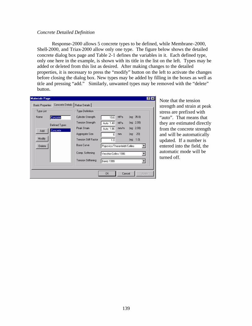
139

Concrete Detailed Definition

Response-2000 allows 5 concrete types to be defined, while Membrane-2000, Shell-2000, and Triax-2000 allow only one type. The figure below shows the detailed concrete dialog box page and Table 2-1 defines the variables in it. Each defined type, only one here in the example, is shown with its title in the list on the left. Types may be added or deleted from this list as desired. After making changes to the detailed properties, it is necessary to press the “modify” button on the left to activate the changes before closing the dialog box. New types may be added by filling in the boxes as well as title and pressing “add.” Similarly, unwanted types may be removed with the “delete” button.

Note that the tension strength and strain at peak stress are prefixed with “auto”. That means that they are estimated directly from the concrete strength and will be automatically updated. If a number is entered into the field, the automatic mode will be turned off.

140

Table 2-1 Concrete Material Properties, Meanings and Default Values

The listed “default value” is selected automatically when using the “basic properties” page of the dialog box.

Property Definition Title Default Value Cylinder Strength Concrete cylinder strength fc' 40 MPa

Tension Strength Tensile strength of concrete ft 0.45(fc')0.4 MPa This should not be modulus of rupture, but rather a value

such as the ACI shear cracking stress

Peak Strain Strain at peak stress e0 As listed in Ref 5 this value, fc', and base curve define stiffness Page 63

Aggregate Size Maximum Aggregate size Maxagg 19 mm (3/4 inch) Used for shear on crack calculations. Reduced

for high strength concrete to model smooth cracks

linearly reduced to 0 mm from 60-80 MPa

Tens. Stiff factor Relative amount of tension stiffening. tsfactor 1.0

Base Curve Basic shape of concrete base curve: Linear linear to (ε0,fc'), zero after Parabolic Parabolic through (ε0,fc') and (2ε0,0) Popovics/Thorenfeldt/

Collins Default equation from Ref (5)

Segmental User defined curve: See Section 5-5 Elasto-Plastic linear to (ε0,fc'), constant at fc' until 2 x ε0

141

TABLE 2-1 (Continued) Compression Models lowering of concrete strength with increasing transverse tensile strain

Softening There are many models here. For normal strength concrete, the Vecchio-Collins 1986 model is suggested. For very high strength concrete (>90 MPa), the Porasz-Collins 1989 model is recommended.

None No change in compressive capacity with tensile strain This option does not model concrete well Vecchio-Collins 1982 Equation proposed by Vecchio, Ref 3 This works well for normal and low strength concrete Vecchio-Collins 1986 Equation proposed by Vecchio/Collins, Ref 1 This is a simplification of the above equation: Recommended Vecchio-Collins 92-A Equation proposed by Vecchio/Collins, Ref 6 This is a new fit to the data. Comparable to the 1982 eq. Vecchio-Collins 92-B Equation proposed by Vecchio/Collins, Ref 6 This is a new fit to the data. Comparable to the 1986 eq. Mehlhorn et al Equation proposed by Mehlhorn et al, Ref 7 This does not model concrete well for high strains Maekawa et al Equation proposed by Maekawa, et al 8 Noguchi et al Equation proposed by Noguchi, et al 9 Belarbi-Hsu proportional Rotating Angle Softened Truss Model Relation

Ref 10. If this is selected with Tamai tension stiffening, program runs in RA-STM mode.

CAN CSA S474 Offshore Code. Like V-C ’86 but Not a function of e0 Collins 1978 Compression Field Theory Equation Ref 11. Kaufmann-Marti 1998 Equation proposed by Kaufmann and Marti Ref 12 This is fit to many RC panels from Canada/Japan/USA Porasz-Collins 1988 Equation proposed by Porasz and Collins Ref 13 Recommended method for very high strength concrete Hsu-Zhang 1998 Model of RA-STM 98 and FA-STM98. Ref 14 Concrete crushes early in this model. Not recommended Hsu 1993 Another model from the Houston RA-STM. Ref 15

Tension Models the post cracking tensile strength in reinforced/prestressed concrete Stiffening The Bentz-1999 model is suggested.

None Ignore post cracking tension stiffening Vecchio-Collins 1982 Equation proposed by Vecchio Ref 3 Collins-Mitchell 1987 Equation proposed in 1987 textbook Ref 16 Suggested Equation if Bentz 1999 method not used Izumo et al Equation proposed by Izumo et al 17 Tamai et al Tamai, also used by Hsu models 18 Elasto-Plastic Full cracking stress at any strain after cracking Bentz 1999 Tension stiffening based on strain and distance to steel

See Reference 2 to find out how this works Reinforcement Detailed Definition

142

Non-prestressed steel is defined in a similar manner to that above for concrete. Note that the example shown has 2 different types of steel defined. The values currently shown at the right are for the selected “x-steel” type. Clicking on the “y-steel” type would allow that to be edited as well.

The “predefined type” option allows selection from common types of steel defined in Table 2-2, below, along with all the other parameters used in this dialog box.

Table 2-2 Reinforcement Material Properties Meanings and Default Values

Property Definition Title Default Value

Elastic Modulus Stiffness before yield E 200,000 MPa Yield Strength Proportional limit fy 400 MPa e-strain harden Strain at strain harden εsh 7 mm/m Rupture strain Strain at Ultimate stress. εu 10%

Ultimate strength Maximum stress fu 1.5 x fy

Curve is linear to yield, flat post yield, and quadratic after strain hardening. Slope is zero at location of maximum stress and strain.

Predefined Options

E fy εsh εu fu

(MPa) (MPa) (mm/m) (mm/m) (MPa) ASTM A615 40 ksi 200000 276 20.0 120.0 483 ASTM A615 60 ksi 200000 414 15.0 80.0 621 ASTM A706 60 ksi 200000 414 15.0 120.0 552 CSA G30.12 300 MPa 200000 300 20.0 110.0 450 CSA G30.12 400 MPa 200000 400 15.0 80.0 600 CSA G30 400 Weld 200000 400 15.0 130.0 550 1030 MPa Dywidag 200000 800 10.0 40.0 1030 1080 MPa Dywidag 200000 820 10.0 40.0 1080

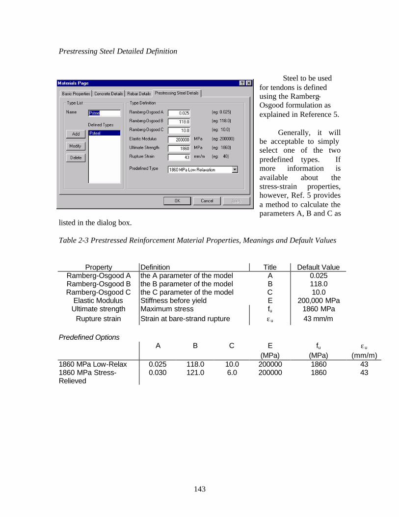
143

Prestressing Steel Detailed Definition

Steel to be used for tendons is defined using the Ramberg-Osgood formulation as explained in Reference 5.

Generally, it will be acceptable to simply select one of the two predefined types. If more information is available about the stress-strain properties, however, Ref. 5 provides a method to calculate the parameters A, B and C as

listed in the dialog box. Table 2-3 Prestressed Reinforcement Material Properties, Meanings and Default Values

Property Definition Title Default Value

Ramberg-Osgood A the A parameter of the model A 0.025 Ramberg-Osgood B the B parameter of the model B 118.0 Ramberg-Osgood C the C parameter of the model C 10.0

Elastic Modulus Stiffness before yield E 200,000 MPa Ultimate strength Maximum stress fu 1860 MPa

Rupture strain Strain at bare-strand rupture εu 43 mm/m

Predefined Options A B C E fu εu

(MPa) (MPa) (mm/m) 1860 MPa Low-Relax 0.025 118.0 10.0 200000 1860 43 1860 MPa Stress-Relieved

0.030 121.0 6.0 200000 1860 43

144

2-5 Longitudinal Reinforcement

Defining longitudinal steel for Membrane-2000 is identical to Shell-2000 and both are similar to Response-2000 and so all will be explained together.

Steel in the programs is defined either as individual layers of bars or in collections of patterned layers. Patterns include distributed patterns as well as circular patterns. Membrane-2000 and Shell-2000 don’t allow circular patterns.

Each dialog box uses the traditional list of layers with the ability to add a new definition, modify an existing one or delete it. This is the same style used in the materials definition page. Individual Layers

Shown is the

Response-2000 longitudinal reinforcement definition page. Membrane-2000 and Shell-2000 are similar except that they ask for spacing of bars rather than the number of bars as well as asking for a prestrain for the bar.

In the example, three layers are defined,

with the one called “bot2” currently highlighted. It has 3 bars defined each with a cross sectional area of 440 mm2 and a centroid 38 mm above the bottom of the cross section. The type of steel selected is “botlong” which would have been defined in the materials dialog page. Different layers can, of course, use different material types.

Table 2-4 shows the bar types built into the programs. See section 5-8 for a description of how to add new bar types to this listing.

145

Table 2-4 Reinforcing Bar and Strand Designations CSA Reinforcing Bars. CSA Prestressing Strands

Bar

Designation Nominal

(mm) Cross

Sectional Area (mm2)

Strand Designation

Nominal Diameter

(mm)

Cross Sectional

Area (mm2) 10M 11.3 100 S9 9.53 55 15M 16.0 200 S11 11.13 74 20M 19.5 300 S13 12.70 99 25M 25.2 500 S13FAT 13.9 107.7 30M 29.9 700 S13S 13.9 107.7 35M 35.7 1000 S15 15.24 140 45M 43.7 1500 55M 56.4 2500

CSA Reinforcing Alternate Titles. US Prestressing Strands (270 ksi)

Bar

Designation Nominal Diameter

(mm)

Cross Sectional

Area (mm2)

Strand Designation

Nominal Diameter

(mm)

Cross Sectional

Area (mm2) 10 11.3 100 S.25 0.250 0.036 15 16.0 200 S.375 0.375 0.085 20 19.5 300 S.5 0.500 0.153 25 25.2 500 S.5FAT 0.550 0.167 30 29.9 700 S.5S 0.550 0.167 35 35.7 1000 S.6 0.600 0.215 45 43.7 1500 55 56.4 2500

Standard US bars Deformed Prestressing Bars (Dywidag)

Bar

Designation Nominal Diameter

(mm)

Cross Sectional

Area (mm2)

Bar Designation

Nominal Diameter

(mm)

Cross Sectional

Area (mm2) #2 0.248 0.050 PB15 15.0 177 #3 0.375 0.110 PB26 26.5 551 #4 0.500 0.200 PB32 32.0 804 #5 0.625 0.310 PB36 36.0 1018 #6 0.750 0.440 #7 0.875 0.600 #8 1.000 0.790 #9 1.128 1.000

#10 1.270 1.270 #11 1.410 1.560 #14 1.693 2.250 #18 2.257 4.000

146

Table 2-4 Reinforcing Bar and Strand Designations (con’t) US Proposed Metric Titles Bars nominal by diameter

Bar

Designation Nominal Diameter

(mm)

Cross Sectional

Area (mm2)

Bar Designation

Nominal Diameter

(mm)

Cross Sectional

Area (mm2) M10 9.5 71 1 mm 1 0.785 M13 12.7 129 2 mm 2 3.142 M16 15.9 200 3 mm 3 7.069 M19 19.1 284 4 mm 4 12.57 M22 22.2 387 5 mm 5 19.63 M25 25.4 510 6 mm 6 28.27 M29 28.7 645 7 mm 7 38.48 M32 32.3 819 8 mm 8 50.27 M36 35.8 1006 9 mm 9 63.62 M43 43.0 1452 10 mm 10 78.54 M57 57.3 2581 11 mm 11 95.03

12 mm 12 113.1 Japanese Bars 13 mm 13 132.7

14 mm 14 153.9 Bar Nominal Cross 15 mm 15 176.7

Designation Diameter Sectional 16 mm 16 201.1 (cm) Area (cm2) 17 mm 17 227.0

JD6 0.64 0.32 18 mm 18 254.5 JD8 0.80 0.5 19 mm 19 283.5 JD10 0.95 0.71 20 mm 20 314.2 JD13 1.27 1.27 21 mm 21 346.4 JD16 1.59 1.99 22 mm 22 380.1 JD19 1.91 2.87 23 mm 23 415.5 JD22 2.23 3.87 24 mm 24 452.4 JD25 2.55 5.07 25 mm 25 490.9 JD29 2.86 6.42 26 mm 26 530.9 JD32 3.18 7.94 27 mm 27 572.6 JD35 3.50 9.57 28 mm 28 615.8 JD38 3.82 11.4 29 mm 29 660.5 JD41 4.14 13.4 30 mm 30 706.9

31 mm 31 754.8 32 mm 32 804.2 33 mm 33 855.3 34 mm 34 907.9 35 mm 35 962.1 36 mm 36 1018

147

3-5 Response-2000

Loading

Response-2000 allows axial load, moment and shear to be applied to the element. Positive axial force is tension and negative axial force is compression. Positive moment indicates compression on the top of the section. The shear term must be positive.

Like all the programs, loading is provided on the left side for a starting load level or a single load analysis, and on the right for the increments in load. The actual magnitudes of the incremental values are not important. Response-2000 only uses the signs and values relative to each other.

For this example, there is no initial load level, and the moment to shear ratio is 1.34 feet.

Time Dependent Effects

To assist in the examination of time-dependent effects, Response-2000 includes a routine that implements the AASHTO-9419 suggested methods for shrinkage, creep and prestressing strand relaxation. This is accessed via the “Loads | Time Dependent Effects” menu option. Note that it does not model the increase in concrete strength with time, as that is too dependent on individual mix designs.

This module will only

be used if the checkbox at the top is selected. The age for long-term behaviour is needed, as is the sustained moment for the section as that strongly affects the creep.

Briefly, the shrinkage and relaxation is estimated for the given age and the

creep under the given sustained moment is estimated. Then a shrinkage/thermal profile is automatically added to the section to model this. Analyses done then represent short term loading on a well-aged beam or column. For a more detailed description of the time-dependent effects module, see Reference 2.

148

Detailed Shrinkage and Thermal Strains

To account for structures such as large box-girders where there is a substantial thermal gradient over the depth of the structure, Response-2000 allows this to be selected with some detail.

Note that the

shrinkage and thermal strains calculated above in the time-dependent effects are not reflected here.

The left side of the dialog box allows selection of values of shrinkage at selected depths. Response-2000 parabolically interpolates between these points.

The top right side allows setting of individual thermal strains for the reinforcement. As shown, it is also possible to select a value and apply it to all layers of reinforcement. Note that these strains can be used the same way as prestrains are to tendons if desired.

The bottom right shows a plot with a line indicating the shrinkage distribution and with little dots to indicate the thermal strains of the reinforcement.

The example shows a 120 inch high section with a large distribution of thermal strains in the top as well as a small distribution in the bottom. The reinforcement does not have any thermal strains defined for it.

149

Strain Discontinuity

The strain discontinuity dialog box allows modelling of behaviour effects due to composite construction. See section 5-7 for a description and example of how best to use the strain discontinuity feature. In general, it allows for an explicit difference between the longitudinal strain profile at a given depth and the basic assumption that plane sections remain plane.

The interface is

similar to the shrinkage page above. Elevation-strain pairs are added to the list and they are plotted on the graph at the right.

In this example, a 2300 mm precast section was given a 200 mm slab on top and the strain discontinuity models the difference from plane-sections for

this slab. Full Member Properties

A full member analysis will calculate force deflection relationships for simple beams. The beam must be prismatic with the load applied at the right end and a support at the left end. Response-2000 requires the length subjected to shear, the length with no shear at midspan (for beams loaded with 2 point loads), the type of loading (point load, UDL beam type or UDL footing type), and the moment at the left end relative to the right end. For a beam type analysis, the left end moment is often equal to zero, as this is where the support would be.

150

The left side support may be selected as a support on the bottom of the beam, a hanging support from the top of the beam, or a fixed support. In addition to changing how the beam is drawn, the left support changes the assumed load sharing between strut action and sectional action in the analysis.

The right side has similar options. In this case, the fixed support also needs information about the penetration of strains into the bottom block of concrete that would be supporting the column. The default value of 0.022 is suggested for columns. See Reference 2 for an explanation of how this is used.

151

4-2 Types of Analyses

Three types of analysis are common to all the programs. The first is the “Full-Response” type of analysis. This will first do a single- load level analysis at the values in the left column of the “Loads | Loads” menu choice, and then increase loads in the ratio shown in the right column of the “Loads | Loads” menu item.

The second type of analysis is a “Single Load Level”. This will solve to the loads selected in the left side of the “Loads | Loads” dialog box.

The third type of analysis is a strain state analysis that will return the stress and force state that corresponds to a given set of global strains.

Membrane-2000 also includes explicit options in the solve menu to perform a full analysis for a number of analysis types. These include the Modified Compression Field Theory 1987 (MCFT)1, the Rotating-Angle Softened Truss Model (RA-STM) 199315, the RA-STM 199510, the RA-STM 199820 , the Fixed Angle Softened Truss Model (FA-STM) 199621 , FA-STM 199722 and FA-STM 199823. Hsu and colleagues at the University of Houston derived the last 6 methods. They are included in Membrane-2000 for comparison purposes. In general, the six methods from Houston do no better a job than the MCFT, despite having much more experimental data to derive from. Response-2000 has a number of additional analysis options:

Full Sectional Response Calculate Moment Curvature as above More Detail Interpolate full sectional response to more detail Member Response Calculate load-deflection relations for simple beams One Load Calculate strains for given M, N, V as above 2 Strain Calculate stress state for given pair of long. strains 1 Strain Calculate stress and strain state corresponding to selected strain at certain depth. (e.g. first yield) M-N Interaction Calculate axial load-moment interaction envelope M-V Interaction Calculate moment-shear interaction envelope. (this is a first step in the Member Response option) N-V Interaction Calculate axial load-shear interaction envelope.

The following section gives a listing of all the 9-plot settings available in the programs. In each case, an example is shown and the description of the 9 plots provides guidance in interpreting analyses. The units listings that goes with each description shows the units used for SI metric, US customary units, and kg-cm units as used in Japan.

152

4-4 Response-2000 Response-2000 9 Plots General

Response-2000 draws plots over the depth of the beam of column. This example shows a sectional analysis with shear and moment on a prestressed single-Tee beam.

Response-2000 uses two control plots. They are selected based on the type of

loading, but for shear analyses, the top one shows shear versus shear-strain plot and the bottom one shows the moment curvature plot. This quickly allows detection of shear failures versus flexural failures. In this case, due to the prestressing, the moment curvature never actually reaches a positive curvature, but the shear plot has started descending indicating a shear failure, in this case before even full depth cracking of the section. The plots show the behaviour just before failure. Cross Section The cross section is drawn darker in regions where the concrete hasn’t cracked. Longitudinal reinforcement and stirrups are draw dark red if on the yield plateau, bright red if strain hardening, and dark and bright green for yielding in compression. In this case, note that despite the positive moment on the section, the bottom of the section hasn’t cracked through yet due to the prestress force.

153

Longitudinal Strain Longitudinal strain (x 10-3) vs section depth This confirms that the curvature is still negative in the section. Note that the line is linear, showing the implicit assumption that plane sections remain plane. Right clicking on this plot and selecting “toggle text” will show or hide the curvature of the beam. Transverse Strain Bulging strain (x 10-3) vs depth of section While the longitudinal strains must be linearly distributed, the transverse strain depends on the local stress-strain conditions at each point in the depth of the beam. They are dictated by the assumption that the total vertical stress at every depth of the beam must be zero. In this failure condition note the high strains (~ 3 x yield strain) near the top of the web. Crack Diagram This plot shows the estimated crack pattern as well as crack widths (mm, in, cm). Note that the crack widths as well as patterns are rather approximate and should not be used alone to estimate the health of a structure. For this beam about to fail, the maximum crack width is predicted to be 3.0 mm. For cases where part of the concrete is crushing, the section is redrawn in pink, and for sections where the cracks are slipping causing failure, the section is drawn in purple. Shear Strain (x 10-3) Like the transverse strain, this shows the distribution of shear strain in the section. If the section starts to unload for any reason, a grey envelope will show the maximum value attained so far. Shear Stress (MPa, psi, kg/cm2) Shear stress is calculated in Response-2000 by a process that considers the longitudinal stiffness of the cracked concrete2. This produces a calculated shear stress profile for each load level. This calculated shear stress profile is shown on the plot in green, and the stress from the strain state is shown in blue. Generally these two lines will match very closely, but if they don’t, the load stage should be treated with some caution. Note that the shear stress is zero at the top and bottom faces of the beam as expected, but that the shear stress distribution isn’t the width-modified parabola that linear theory would predict. The calculated shear-stress profiles for cracked reinforced concrete in general are more complex than linear theory would predict, having important effects on predicted behaviour. Principal Compressive Stress (MPa, psi, kg/cm2)

Principal compressive stress over the depth is shown in the bottom left. The maximum allowable stress is shown in red at left. This number will reduce due to cracking in the concrete as predicted by the MCFT. The blue line is the applied stress in the concrete at each depth in the beam. Note that due to the shear inducing diagonal compression, it is quite possible to have principal compression over the entire depth of the beam. The stress in this beam is more due to the prestressing, however. If the red and blue lines touch, the concrete is predicted to crush and the section will fail. That is

154

the fate of this beam. At the next load stage, the concrete is crushing at the top of the web. Shear on the Crack (MPa, psi, kg/cm2) Cracked concrete may require shear on the crack to maintain the principal tensile stress in the concrete. See the Membrane-2000 section above for a discussion of this. As in that section, the maximum allowable shear on the crack is shown in red with the applied in blue. For this section, the maximum is limiting the shear on the crack over part of the depth. In that region, the principal tensile stress has been lowered to maintain equilibrium. Principal Tensile Stress (MPa, psi, kg/cm2) This tensile stress will exist throughout the beam, caused by shear on the cross section. Note the location where the stress is reduced due to the shear on the crack limitation. The red line on the right indicates the maximum value of stress allowed due to the requirement of longitudinal yield. If this line pulls in diagonally and intersects the blue applied stress line, the section is approaching flexural failure. Response-2000 9 Plots Cracking

This page of 9 plots in Response-2000, not shown here, contains plots of: Cross Section as above Longitudinal strain as above Principal tensile strain (x 10–3) Crack diagram as above Crack width plot (mm, in, cm) Average Angle with depth (degrees) Longitudinal Crack Spacing (mm, in, cm) Transverse Crack Spacing (mm, in, cm) Diagonal Crack Spacing (mm, in, cm)

Response-2000 calculates crack spacing based on the angle and the estimate of crack spacing in the longitudinal and transverse directions as per the MCFT. If the crack spacing is calculated automatically as suggested, the spacing will vary over the depth of the section, further improving the realism of the analysis. Response-2000 9 Plots Reinforcement

This page shows the state of the reinforcement in the longitudinal and transverse direction. The following plots are included: Cross Section as above Longitudinal strain as above Transverse strain as above Longitudinal Reinforcement Stress (MPa, ksi, t/cm2) This the average stresss

155

Longitudinal Reinforcement Stress at a crack (MPa, ksi, t/cm2) This local value includes the effects of the shear on the crack and principal tension. Longitudinal Average Bond (MPa, psi, kg/cm2) This bond stress is what the reinforcement must be able to withstand in order to support the given shear. No limitations are made in Response-2000 if this value becomes unrealistically high. Stirrup Stress (MPa, ksi, t/cm2) This shows the average stress in the stirrups over the beam depth. Stirrup Stress at a Crack (MPa, ksi, t/cm2) This is the local stress at a crack mandated by equilibrium considering shear on the crack and principal tensile stresses. Transverse Average Bond (MPa, psi, kg/cm2) As the stress is changing along the length of the stirrups, it is possible to calculate the bond stresses that would need to be resisted by the stirrup. Response-2000 calculates these but does not use them to affect the analysis at all. In cases where a stirrup enters the top flange of a T-Beam, for example, there will be a large drop in stirrup stress due to the increased concrete area, resulting in a very large calculated bond. The real bond would be much lower due to strain penetration, and shear lag of forces entering the top flange.

156

Response-2000 9 Plots No Shear

For analyses without any shear, Response-2000 automatically shows a special 9-plot page for that case shown below for a beam under axial compression and shear.

This page has 2 new graphs that have not been explained yet.

The Internal Forces plot shows the force and location of the compressive and tensile forces in the cross section. In this case, due to the axial load, they do not balance each other. Note that the tensile force arrow may not come directly from the steel location due to the concrete tensile force component. By right clicking on the plot, another mode may be selected that calculates directly the resultant of the steel and concrete forces. This can produce counterintuitive results, so isn’t the default mode of presentation.

The N+M plot shows the moment and axial force drawn simply as arrows. This helps in finding mistakes in simple things such as the sign of the axial force.

157

Response-2000 Load Deformation Plots

The example below shows the screen of Response-2000 in the load-deformation plot mode. The figure shows the AASHTO-99 moment-shear interaction diagram for a column tested at the University of Toronto in the 1970’s by Aregawi24 . This figure contains a great deal of information and so will be explained in detail.

Response-2000 Interface Issues

This page of results is selected with the toolbar icon with the lamba (λ − signifying load factor) beside the little 9-plot icon or from the “View | Load Deformation Plot” menu.

The background plot is selected in the top left of the screen. Currently it is selected to the AASHTO-99 LRFD M-V interaction diagram. Below that option is the “Paste Data” section that allows selection of which plots to paste onto the plot. The figure at the start of the section showing cracked shell elements on the main figure was prepared this way with Shell-2000. Currently selected is the longitudinal strain profile, with the current levels controlled by the control plot below. Pressing the “add to graph” button would paste the picture on the main figure where it could be moved and resized.

The main figure contains a pair of text-boxes as well as a diagram of the element. The element picture is pasted on via the “Options | Insert Beam Diagram” menu option. By right clicking on the figure, the dimension text may be resized and copied to the

158

clipboard etc. The top text was automatically prepared by Response-2000 and inserted with the “Options | Insert Text Box” option. This text box may also be edited and customised. The bottom right text box was automatically included by Response-2000 to provide information on how the AASHTO-99 analysis was calculated. Analysis Results Issues

The AASHTO-99 page (there is also an AASHTO-94 LRFD page) automatically calculates the strength of the section and prints it in the text box, in this case in the bottom right. It can be seen that the ultimate shear capacity (Vu) was predicted as 79 kips. This is calculated for the ratio of moment to shear selected from the “Loads | Loads” dialog box. Note that there is a little box on the interaction curve at the point it calculates failure at. In this case, it is on the top curve part of the envelope meaning a shear failure is predicted.

There is an additional little box shown just below the envelope, this is the maximum load that the Response-2000 analysis was able to achieve. In this case they are very close, but they can vary more widely. If the Response-2000 prediction is outside the envelope, it suggests that the AASHTO code is conservative compared to the more advanced predictions that Response-2000 makes. If the Response-2000 prediction is within the envelope, it suggests that the code is unconservative compared to the Response-2000 analysis. This provides a second, independent, checking of the provisions of the code that can add to engineer’s confidence for strength predictions of unusual geometry.

It is noted in the top text box that this particular column happened to fail experimentally at a shear of 80 kips, which is in excellent agreement with both the Response-2000 predictions and the code prediction. See Reference 2 for more discussion of the experimental verification of Response-2000.

159

Other Load-Deformation Plots

Response-2000 also has the following load-deformation plots. Shear/Moment VS longitudinal strain at mid-depth Moment-Curvature Moment-Maximum Crack Width Moment-Maximum Reinforcement Strain Shear-Maximum Crack Width Shear-Shear Strain Shear-Transverse Strain Interaction Diagrams (M-V, N-V, M-N depending on which is calculated) Response-2000 Full Member Plots

One of the features of Response-2000 is that while internally it is a sectional

analysis program, it is able to connect a number of sections to perform simple member analysis. The shown example is for the largest beam ever tested in shear, tested by Shioya et al in Japan25. This beam had an effective depth of 3000 mm (10 feet), and was 36 metres long (120 feet). The beam was subjected to a uniformly distributed loading.

To perform the shown Response-2000 analysis, the section was first entered into the program. Next, the “Loads | Full Member Properties” option was used to select a length of 18 metres (Response-2000 does the analysis on the half- length of the beam),

160

and the loading was switched to a uniformly distributed load. Finally, the “Solve | Member Response” menu option was selected.

Response-2000 calculated the interaction diagram shown in the top control chart. It then determined the la rgest loading envelope that would fit into the diagram. It can be seen that the loading envelope touches the failure envelope on the top indicating a shear failure. If it had touched at the right side, it would have represented a flexural failure. The shape of the loading envelope is parabolic on the right and linear on the left. See Reference 2 for a description of the derivation of the loading shape.

The shown crack diagram is the predicted extent of cracking in the beam at failure. The support plate can be seen on the left. The loading is uniform over the top surface of the beam. Using the lower control plot, the predicted extent of cracking at other load levels may also be explored.

The plots at the bottom are also instructive. The top left one shows the change in curvature over the length of the beam. The location of first flexural cracking, about 2500 mm from the support, can be clearly seen as can the roughly parabolic distribution that would be expected for the parabolic moment diagram. Note that these curvatures all implicitly include the effect of shear on the curvature.

The shear strain distribution shows that the average shear strain over the length of the beam isn’t uniform at all. It may be expected that the strain would increase linearly from the right as the shear diagram is linear, but this isn’t the case due the concrete non-linearity. The strong interaction of shear and moment for this beam means that the predicted critical location for shear is about 6 metres away from the location of maximum shear.

Rounding out the plots are the predicted deflected shape and the plot of load

versus deflection for the beam. Note that the failure is predicted at a load of 102.6 kN/m and a deflection of about 100 millimetres. The experimental failure load was measured as 105 kN/m, at a deflection of about 100 millimetres.

161

5-8 Rebar.dat

Each of the programs has a list of reinforcing bar definitions that can be used by any cross section (see Table 2-4 in section II). This list is, in fact, user definable. Each program maintains a file in its install directory called “rebar.dat” that is a text file loaded each time the program starts. Users may add to this list and the new options will be available the next time the program is started. Note that each program has a separate rebar.dat, but they are all identical on distribution. (i.e. if changes are made to one, they can be copied to the directories of the other programs as well.) The format of the file is as follows: // Response-2000 Data File // // This file contains the definitions of all standard rebar/strand types // // Users may add more types which will be available the next time that // Response-2000 is started. Input is not case sensitive. // // If bars are entered with the same name as existing ones, the first one will be used // Bar title is limited to 14 characters. Spaces are allowed, but the first number // found after the title and a space is assumed to be the area. // // Information is as follows: // // Name code Nominal Diameter (mm) Nominal Area (mm^2) // // -- start of default listing -- // // CSA standard Reinforcing Bars // 10M 11.3 100 15M 16.0 200 20M 19.5 300 25M 25.2 500 30M 29.9 700 35M 35.7 1000 … etc

If a file including a user defined bar is used on a version of one of the programs that has not seen the bar title before, the new name will be saved to the standard listing when the program shuts down.