Fatigue Life Prediction of Screw Blade in Screw Sand...

© 2016 Jie Gong, Yun-Fei Fu, Wen Xia, Ji-Hua Li and Fan Zhang. This open access article is distributed under a Creative

Commons Attribution (CC-BY) 3.0 license.

American Journal of Engineering and Applied Sciences

Original Research Paper

Fatigue Life Prediction of Screw Blade in Screw Sand

Washing Machine under Random Load with Gauss

Distribution

Jie Gong, Yun-Fei Fu, Wen Xia, Ji-Hua Li and Fan Zhang

Agricultural Product Processing Research Institute at Chinese Academy of Tropical Agricultural Sciences, Zhanjiang524001,

China

Article history

Received: 24-11-2016 Revised: 27-11-2016 Accepted: 21-12-2016 Corresponding Author: Wen Xia Agricultural Product Processing Research Institute at Chinese Academy of Tropical Agricultural Sciences, Zhanjiang524001, China Email: [email protected]

Abstract: The purpose of this study is to present a new method for estimating the fatigue life of the screw blade in the screw sand washing machine. To ensure the accuracy of numerical simulation, the loading area and the value of load are determined by means of the theoretical analysis. To ascertain the location of the stress peak and stress range, the static analysis of the screw blade is executed via the finite element method. To reduce the research cost and ensure the feasibility of the research method, Markov chain Monte Carlo (MCMC) is employed to simulate the random load with the Gauss distribution on the screw blade. In addition, the Nondominated Sorting Genetic Algorithm (NSGA-II) is utilized to find out an optimum variation coefficient of the stress, aiming at guaranteeing the precision of the random load. The rainflow cycle extrapolation is adopted to generate the fatigue load spectrum closer to the real condition, taking account of the possibility of the extreme loads caused by overload occurrence. Subsequently, the rainflow matrix after extrapolation, the estimated P-S-N curve, Goodman stress correction method and Miner’s rules are made use of assessing the service life of the screw blade. In particular, the effects of the surface roughness, residual stresses and fatigue notch factors on the fatigue life are taken into consideration. Ultimately, the non-linear surface fitting technique is used to obtain the equation concerning the fatigue life of the screw blade versus residual stresses and fatigue notch factors. The numerical results show that the stress peak is in the root of the screw blade and the service life of the screw blade declines exponentially with growing residual stresses and fatigue notch factors. Keywords: Fatigue Life, Markov Chain Monte Carlo, NSGA-II, Rainflow Cycle Extrapolation, Non-Linear Surface Fitting

Introduction

With the increasingly rapid development of the architectural industry throughout the world, the demands for the sand used as the concrete fine aggregate are extremely huge (Zhang et al., 2010; Shi et al., 2012). Recently, river sand is a main source of sand for building, whereas river sand resources are surprisingly dwindling due to resource and environment constraints. Worldwide, since numerous coastal cities have a vast number of sea sand resources, the development and

utilization of sea sand resources will therefore resolve the contradiction between the limited river sand resources and the urban growth. In comparison with river sand, the chloride salt and shell in sea sand are two major factors restricting the application of sea sand. Researches have shown that the chloride salt in sea sand will have negative effects on the hydration process of the portland cement and will corrode the steel bar in concrete and the shell in sea sand will adversely affect the durability of concrete (Vedalakshmi et al., 2008). As a result of misusing sea

Jie Gong et al. / American Journal of Engineering and Applied Sciences 2016, 9 (4): 1198.1212 DOI: 10.3844/ajeassp.2016.1198.1212

1199

sand, a series of severe engineering accidents have unfortunately occurred in several countries, such as Japan, Britain, China, Turkey, etc. Nowadays, various sand washing technologies have been adopted to clean sea sand, to acquire qualified sea sand that can be used in the construction industry.

Currently, mechanical sand washing methods are wide-spread all over the world, because the working efficiency of mechanical sand washing methods are the highest, compared with the remaining sand washing technologies: The natural cleaning method with fresh water and natural placement method (Fu et al., 2015). More importantly, sand washing machines are the crucial components of mechanical sand washing systems (Fu et al., 2015). Presently, there are three main categories of sand washing machines in diverse mechanical sand washing systems, namely, the screw sand washing machine, rotating wheel sand washing machine and vibration sand washing machine (Fu et al., 2015; Yang et al., 2016). Virtually, the sand washing capacity of the screw sand washing machine far outperforms that of the other two types of sand washing machines (rotating wheel sand washing machine and vibration sand washing machine), so this study takes the screw sand washing machine as the research object (Yang et al., 2016; Fu et al., 2016). In most mechanical sand washing systems, the subsystem of eliminating the chloride salt in sea sand is shown in Fig. 1, including screw sand washing machines and the equipment for generating ozone water (Fu et al., 2015). When sand washing machines run smoothly, the ozone water is conveyed into the running screw sand washing machines to get rid of the

chloride salt in sea sand via the pipes (Fu et al., 2015). This means that the chemical approach is taken advantages of desalting the sea sand without consuming the extra energy of screw sand washing machines.

Practically, the screw blade is an actuator of washing sea sand in screw sand washing machines, with the result that it will suffer from the sophisticated alternating load, causing the fatigue damage of the screw blade. The service life is an essential index used for evaluating the performance of screw sand washing machines. On the condition that the screw sand washing machine is out of service in a series mechanical sand washing system, the whole sand washing system would stop working. Under the circumstance that the screw sand washing machine is unable to run in a parallel and series mechanical sand washing system, the output of desalted sea sand would be adversely affected to a large extent. Consequently, the investigation regarding the fatigue life prediction of the screw blade would accelerate the sustainable progress of the sand washing technology to some extent.

Approach for Fatigue Life Prediction

A general approach for predicting the fatigue life of the screw blade is fairly required, which could dramatically cut the research and development expenditure on the screw sand washing machine. The flow diagram of the method mentioned in this study for estimating the fatigue life of the screw blade is illustrated in Fig. 2.

Fig. 1. Subsystem of removing the chloride salt


1200

Fig. 2. Flow diagram of predicting the fatigue life of the screw blade

The chief steps of this approach are summarized as follows: Step 1. Execute the finite element analysis to determine

the stress range in the weakest location of the screw blade.

Step 2. Take advantages of the Markov chain Monte Carlo to generate the random loading on the screw blade.

Step 3. Harness the rainflow cycle counting and extrapolation to produce the random load input used for assessing the fatigue life.

Step 4. Carry out the prediction of the service life allowing for the effects of the surface roughness, residual stress and fatigue notch factor.

Step 5. Utilize the non-linear surface fitting technique to achieve the formula regarding the fatigue life of the screw blade.

Determination of Loading Area and

Magnitude of Load

Determination of Loading Area

As the working principle of the screw sand washing machine closely resembles that of the screw conveyor, the determination of the loading area and the magnitude of the load on the screw blade will refer to the screw conveyor (Fu et al., 2016). Apparently, the main differences between the screw sand washing and screw


1201

conveyor are practical working surroundings and detailed dimension parameters.

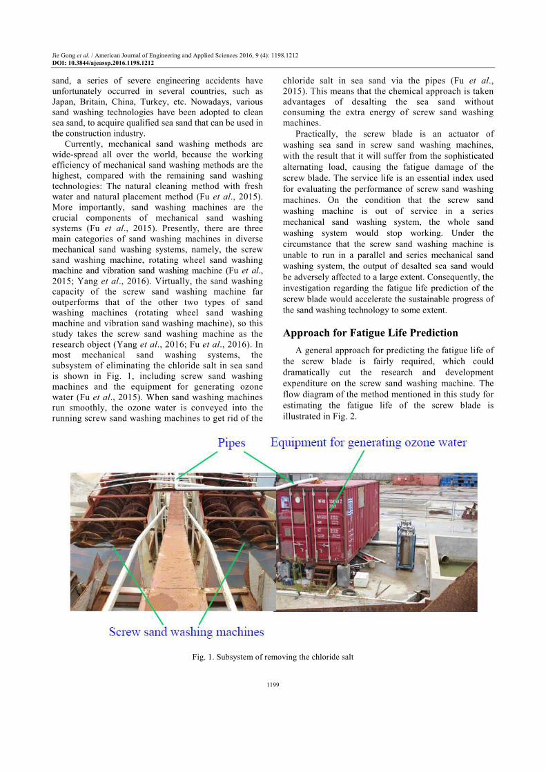
When the filling coefficient of the screw sand washing machine is a constant, the cross section of the sea sand in the feed through is similar to arch (Wang et al., 2012b; Pezo et al., 2015). Because of the effect of dynamic friction, there is an angle β between the line OW and the vertical line, as shown in Fig. 3 (Wang et al., 2012b; Pezo et al., 2015). In Fig. 3, the point W is the center of gravity of sea sand, the point O is the axis of the screw axis and the angle θ is the central angle of the cross section of sea sand. In actual engineering, let the angle β be the dynamic friction angle. Based on angles β and θ, the loading area of the screw blade can be determined, as shown in Fig. 3.

The cross-sectional area of sea sand is (Wang et al., 2012b):

g yA Aγ= (1)

But:

( )21sin

8gA D θ θ= − (2)

2

4y

DA π= (3)

Equation 1 then reduces to:

sin 2θ θ γπ− = (4)

Where: Ag = The cross-sectional area of sea sand (m2) Ay = The cross-sectional area of the screw blade (m2) γ = The filling coefficient D = The diameter of the screw structure (m) θ = The central angle of the cross section of sea sand

(rad) Calculation of Load

When the screw sand washing machine washes sea sand, the force condition of the screw blade is intensely complicated (Müller, 2009). To illustrate the force condition of the screw blade clearly, let the center of gravity of sea sand W be the acting point of force (Wang et al., 2012b). The simplified force condition of the screw blade is shown in Fig. 4. In Fig. 4, F is the resultant force in newtons, Fn is the normal force of the screw blade in newtons and Ff is the friction between sea sand and the screw blade in newtons. Also, the resultant force F can be broken into the axial force Fa and radial force Fr.

Fig. 3. Loading area of screw blade

Fig. 4. Simplified force condition of screw blade

For applying load in the finite element analysis conveniently, assume that the load per unit area in the loading area of the screw blade is equal. In consequence, the pressure load of the screw blade can be expressed by:

naverage

g

FP

A= (5)


1202

where, Paverage is the pressure load of the screw blade (Pa).

The normal force of the screw blade is:

cosn

F F β= (6)

But:

( )sinrF

Fω β

=+

(7)

arctanS

Dω

π= (8)

1tanβ µ−= (9)

Where: β = The dynamic friction angle (°) ω = The screw angle of the screw blade (°) S = The pitch (m) µ = The friction coefficient between the screw blade

and sea sand

The radial force can be expressed by Fr:

1r

TF

OW= (10)

But:

1 9549s

PST

n L= (11)

3sin4 2

3 sin 2

DOW

θ

θ θ= ⋅ ⋅

− (12)

Where: T1 = The torque of a circle of the screw blade (Nm) OW = The length of the line OW (m) P = The driving power of the screw sand washing

machine (kW) ns = The speed of the screw axis (rad min−1) L = The transportation distance (m)

The driving power of the screw sand washing machine is used to overcome various resistances in the process of washing sea sand. In general, the driving power of the screw sand washing machine can be expressed by (Fu et al., 2016):

sin

367 20 367rQL DL QL

Pµ ε

= + + (13)

Where: Q = The production capacity (ton hr−1) µr = The running resistance factor ε = The installation angle (°)

The production capacity of the screw sand washing machine is given by (Fu et al., 2016):

247s i

Q D Sn Cγρ= (14)

Where: ρ = The material accumulation density (ton m−3) Ci = The inclination factor

As distinct kinds of screw sand washing machines have different technical parameters, this study takes a typical screw sand washing machine as the research object, whose technical parameters are as follows:

3

1

7.5 , 0.82 , 0.71 , 15 ,

1.6 , 0.2, 0.88,

10 min , 1.9, 0.2

i

s r

L m D m S m

ton m C

n r

ε

ρ γ

µ µ

−

−

= = = = °

= = =

= = =

In addition, the diameter of the screw axis d is 0.25 m

and the thickness of the screw blade δ is 0.005 m.

Static Analysis of Screw Blade

Establishment of Finite Element Model

To reduce the simulation time, the simulation model is simplified as a circle of the screw blade. Actually, the high-quality finite element model plays a vital role in the finite element analysis because the high-quality finite element model, in the process of simulation, can reduce errors to minimum (Tsai and Wang, 2015; Zhou et al., 2016; Wu et al., 2016). Accordingly, to guarantee the accuracy of the numerical calculation, let the element size be 3 mm. The finite element model of the screw blade is shown in Fig. 5. According to the statistic data in ANSYS Workbench, it can be seen that the number of nodes is 6824679 and the number of elements is 4738561.

By calculating Equation 4 and 9, angles θ and β are determined, the values of which are 121° and 11.3°, respectively. Depending on angles θ and β, the loading area is determined. By calculating Equation 5, the pressure load of the screw blade is determined, the value of which is 18428 Pa. Furthermore, the material parameters of the screw blade are as follows: The density is 7.85 ton m−3, the young’s modulus is 2×1011 Pa, the poisson’s ratio is 0.3, the yield strength is 240 MPa and the ultimate tensile strength is 440 MPa.


1203

Results of Finite Element Analysis

ANSYS Workbench is used to execute the numerical simulation of the screw blade. The pressure load is applied on the loading area and the fixed supports are applied at both ends of the screw axis. Through the finite element analysis, the stresses of the screw blade are obtained, as shown in Fig. 6. From Fig. 6, it can be seen that the maximum equivalent stress is in the root of the screw blade. The results show that the maximum equivalent stress is 127.23 MPa, which is less than the yield strength of the screw blade (240 MPa). Therefore, the root of the screw blade is the position easy to generate fatigue failures. As a consequence, the root of the screw blade is taken as the research object to estimate the fatigue life. In particular, the equivalent stress in the root of the screw blade is in the range of 27.267 to 127.23 MPa.

Fig. 5. Finite element model of screw blade

Fig. 6. Distribution of stresses of screw blade

As the screw blade performs the periodically rotational motion, the stress distribution in the root of the screw blade, which is shown in the Fig. 6, can exactly mirror the change process of the stress of a point in the root of the screw blade within a rotation period. To put it another way, the stress obtained by the static analysis is able to describe the dynamic change process of a specific point on the screw blade, due to the periodicity of the screw blade.

Generation of Fatigue Load Spectrum

Simulation Method of Fatigue Load

The stress spectrum is the precondition of the fatigue life prediction and also, the practice shows that the fatigue load, in most cases, has some randomness. Owing to the randomness of load, the stress spectrums obtained by different tests still has significant differences, even for the same components. Therefore, the stress spectrum used for calculating the fatigue life should be the statistical results of the measured data obtained by multiple tests. In fact, the generation of the fatigue load spectrum requires large sample numbers of statistically meaningful data sets. However, on account of the restriction of time and resource, it is unable to conduct a great quantity of experimental investigations to generate a huge number of data sets under many circumstances. As a result, it is desirable to have a technique to simulate the fatigue load required by the fatigue life prediction. Because of this, this study takes advantages of statistical theory to simulate the fatigue load of the screw blade.

Monte Carlo methods, especially those based on Markov chains, have now matured to be part of the standard set of techniques used by statisticians (Robert and Casella, 2004). Markov Chain Monte Carlo (MCMC) is a method involving the use of random numbers to achieve data series with given probability distributions on the basis of Markov chain (Wang et al., 2012a). The basis of MCMC is a Markov chain that generates a random walk through the search space and successively visits solutions with stable frequencies stemming from a stationary distribution (Vrugt, 2016). Compared with MCMC, standard Monte Carlo simulation methods are computationally inefficient for anything but very low dimensional problems (Vrugt, 2016). That is, for the large-scale problems with a large number of random variables and sampling sets, it is extremely tough for standard Monte Carlo simulation methods to obtain reliable results. More importantly, because of involving a couple of powerful simulation techniques, MCMC has the ability to generate the random loadings with any given probability distribution (Zio, 2012). Depending on the analysis above, MCMC is utilized to simulate the random load on the screw blade.


1204

Particularly, the Gauss distribution (normal distribution) is the most common and widely used probability distribution, which can be used to describe many natural phenomenon and different physical properties (Xie, 2013). In consequence, assume that the stress in the root of the screw blade follows the Gauss distribution; that is, the fatigue load on the screw blade is a random Gauss-process. In addition, the degree of variation of the loads on the screw blade can be evaluated by the variation coefficient. Therefore, the probability density function of the random load on the screw blade is given by:

( )

2

1

21

2

Sr

Sr

r

x

r

S

f S e

µ

σ

σ π

− − = (15)

But:

max min

2r

r r

S

S Sµ

+= (16)

r r rS S SCσ µ= (17)

Where: Sr = The stress in the root of the screw blade (MPa)

rSµ = The mean value of the stress Sr (MPa)

rSσ = The standard deviation of the stress Sr

Srmax = The maximum value of the stress (MPa) Sr Srmin = The minimum value of the stress Sr (MPa)

rSC = The variation coefficient of the stress

The advantages of using the high sampling frequency

are that the high sampling frequency can not only obtain the peak of the analog signal more accurately but also provide the better time-domain resolution (Lee et al., 2005). On the other hand, the disadvantage of using the high sampling frequency is that a great number of sampling data will prolong the time of the subsequent processing (Lee et al., 2005). Through comprehensive consideration, this study lets the sampling frequency be 1 kHz (Narayanan et al., 2016). Furthermore, according to the speed of the screw axis (10 r min−1), the rotation period of the screw blade can be readily acquired, which is 6 sec (the reciprocal of the speed of the screw axis).

Determination of Variation Coefficient with NSGA-

II

The selection of the variation coefficient of the stress is overwhelmingly paramount because it will affect the accuracy of generating the fatigue load spectrum. To get an accurate fatigue load, the intelligent optimization

algorithm is used to find out the optimal variation coefficient. Given that the minimum and maximum value are the main features describing the random load on the premise of determining the random load distribution, the difference between the minimum value of the fatigue load simulated by MCMC and the minimum value of the stress in the root of the screw blade and the difference between the maximum value of the simulated fatigue load and the maximum value of the stress in the root of the screw blade should be minimum.

Genetic algorithm is a pretty powerful method for the optimization of the non-linear and complex problems that works depending on the natural selection process in biological systems (Gholami and Azizi, 2014). Particularly, the Non-Dominated Sorting Genetic Algorithm (NSGA-II), an extended form of GA, has become one of the most efficient algorithms for the multi-objective optimization in recent years (Chen et al., 2015). Compared with traditional algorithms, NSGA-II could avoid the dependence on selecting proper weight values, which is still a challenging problem (Gholami and Azizi, 2014; Mi et al., 2016). As NSGA-II presents an extremely outstanding performance in the aspect of solving multi-objective optimization problems, this research harnesses NSGA-II to achieve a most appropriate variation coefficient of the stress (Murugan et al., 2009).

The multi-objective problem to be optimized can be expressed as:

( )1 min min:r

r rSMinimize f f C S= − (18)

( )2 max max:r

r rSMinimize f f C S= − (19)

Subjected to:

0 0.5

rSC≤ ≤ (20)

Where: frmin(⋅) = A function used for finding out the minimum

value from the fatigue load frmax(⋅) = A function used for finding out the maximum

value from the fatigue load

The optimization problem for calculating the optimal variation coefficient of the stress has two objective functions and just a variable. Considering the complexity of this multi-objective optimization problem, let the Pareto front population fraction, population size, the number of generations, stall generation limit and function tolerance be 0.3, 100, 200, 200, 1×10−100, respectively. By analyzing calculation results, it is found that the optimal variation coefficient obtained with NSGA-II is 0.182. Through using MATLAB, the statistical histogram of the random


1205

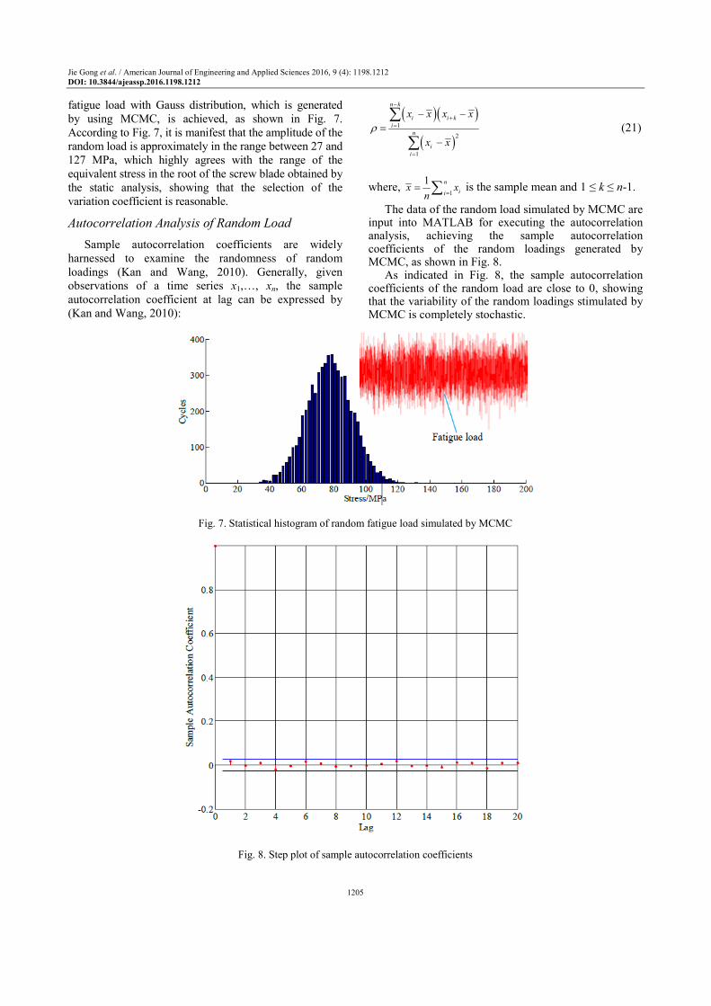
fatigue load with Gauss distribution, which is generated by using MCMC, is achieved, as shown in Fig. 7. According to Fig. 7, it is manifest that the amplitude of the random load is approximately in the range between 27 and 127 MPa, which highly agrees with the range of the equivalent stress in the root of the screw blade obtained by the static analysis, showing that the selection of the variation coefficient is reasonable.

Autocorrelation Analysis of Random Load

Sample autocorrelation coefficients are widely harnessed to examine the randomness of random loadings (Kan and Wang, 2010). Generally, given observations of a time series x1,…, xn, the sample autocorrelation coefficient at lag can be expressed by (Kan and Wang, 2010):

( )( )

( )1

2

1

n k

i i k

i

n

i

i

x x x x

x x

ρ

−

+=

=

− −=

−

∑

∑ (21)

where, 1

1 n

iix x

n == ∑ is the sample mean and 1 ≤ k ≤ n-1.

The data of the random load simulated by MCMC are input into MATLAB for executing the autocorrelation analysis, achieving the sample autocorrelation coefficients of the random loadings generated by MCMC, as shown in Fig. 8.

As indicated in Fig. 8, the sample autocorrelation coefficients of the random load are close to 0, showing that the variability of the random loadings stimulated by MCMC is completely stochastic.

Fig. 7. Statistical histogram of random fatigue load simulated by MCMC

Fig. 8. Step plot of sample autocorrelation coefficients


1206

Fig. 9. Rainflow cycle counting histogram after extrapolation Rainflow Cycle Counting and Extrapolation

Rainflow cycle counting is utilized as a signal processing approach for fatigue analysis (Baek et al., 2008). In practice, rainflow cycle counting is a method of taking a variable amplitude stress history and from it identifying a number of cycles with different range and mean values, which are identified as potentially damaging events (Baek et al., 2008; Johannesson and Thomas, 2001). The rainflow cycle counting of the fatigue load on the screw blade is executed using the Rainflow module in nCode GlyphWorks, an extremely specialist fatigue analysis software.

In many cases, fatigue analysis ignores the possibility of the extreme loads caused by overload occurrence in a longer time period, which is an incorrect postulate actually (Lee et al., 2005). Although extreme loads rarely occur in practical engineering, extreme loads can result in substantial damage of components and have great effects on the final determination of fatigue damage. In consequence, the extreme loads caused by overload occurrence should be taken into consideration. As the aim of the rainflow cycle extrapolation method is to predict the rainflow histogram for a much longer time period based on a short-term load measurement, the rainflow cycle extrapolation method is therefore employed to generate the fatigue load spectrum closer to the real condition (Johannesson, 2006).

According to the recorded field data, the time of transferring sea sand from the flume to discharge opening is around 63 sec. Accordingly, let the extrapolation factor be 10.5; namely, the rainflow cycle counting histogram after extrapolation represents the fatigue load spectrum of 63 sec. Additionally,

Nonparametric Extrapolation method (NPE) is utilized for extrapolation purpose, which uses a nonparametric statistical method to obtain the statistical probability distribution (Wang et al., 2016). The rainflow cycle counting histogram after extrapolation is shown in Fig. 9. Presented in Fig. 9 is the distribution of the stress range and mean stress of the random load in the root of the screw blade. From Fig. 9, it can be seen that the data in the large range region are very sparse. Actually, the rainflow cycle counting histogram after extrapolation is the fatigue load input used for predicting the fatigue life of the screw blade.

Fatigue Life Calculation of Screw Blade

Estimation of P-S-N Curve

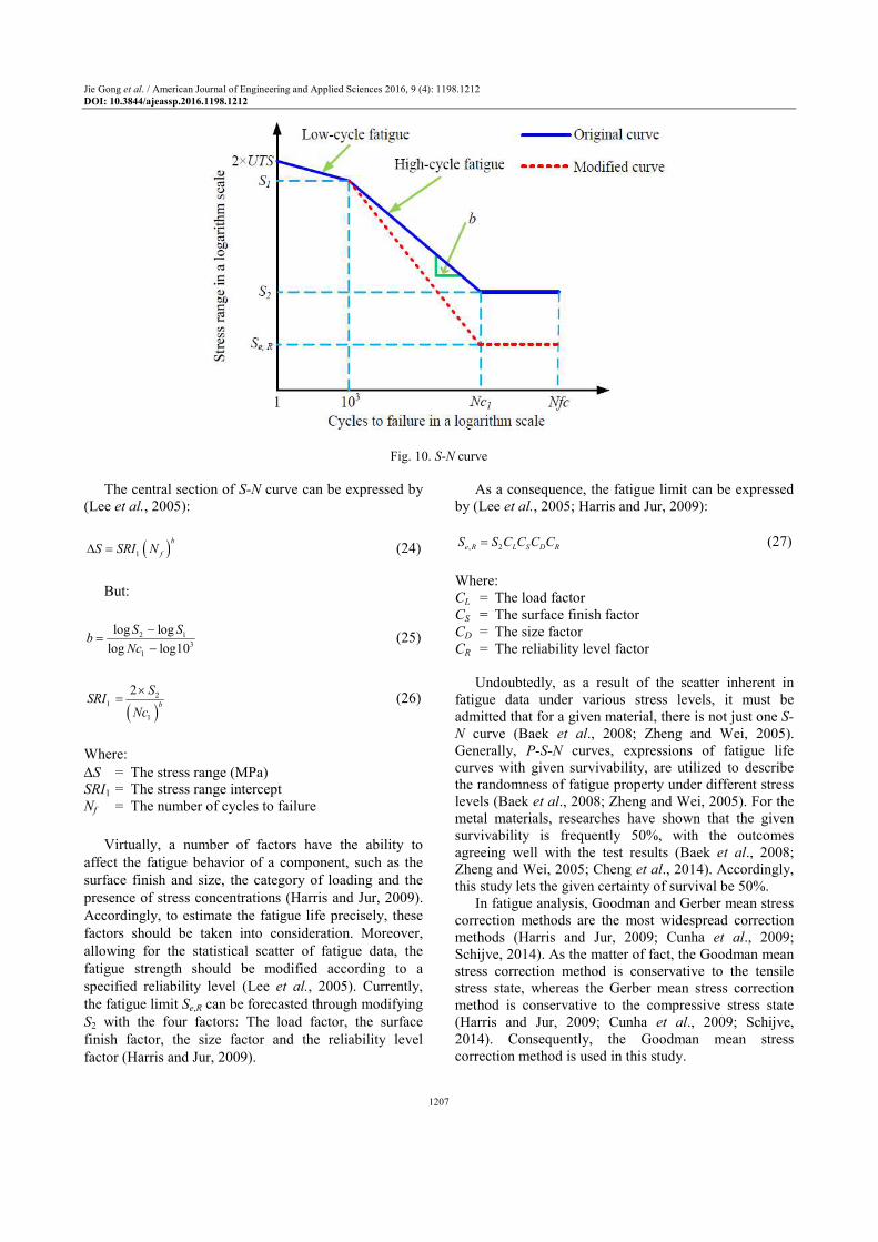
The S-N curve is the foundation of predicting the fatigue life of the screw blade. Generally, the standard S-N curve consists of 3 linear segments on a log-log plot, as shown in Fig. 10. In Fig. 10, is the ultimate tensile strength, b is the slope of the S-N curve in the high-cycle fatigue region, Nc1 is the transition life and Nfc is the numerical fatigue cutoff life, normally set at 1×1030 cycles (Lee et al., 2005). For steels, the transition life Nc1 is normally 106 cycles. Additionally, S1 is the value of the stress at 1000 cycles, S2 is the value of the stress at the transition life Nc1 and Se,R is the fatigue limit.

S1 and S2 can be expressed by the following equations (Lee et al., 2005):

1 0.9S UTS= × (22)

2 0.357S UTS= × (23)


1207

Fig. 10. S-N curve

The central section of S-N curve can be expressed by (Lee et al., 2005):

( )1

b

fS SRI N∆ = (24)

But:

2 13

1

log log

log log10

S Sb

Nc

−=

− (25)

( )2

1

1

2b

SSRI

Nc

×= (26)

Where: ∆S = The stress range (MPa) SRI1 = The stress range intercept Nf = The number of cycles to failure

Virtually, a number of factors have the ability to

affect the fatigue behavior of a component, such as the surface finish and size, the category of loading and the presence of stress concentrations (Harris and Jur, 2009). Accordingly, to estimate the fatigue life precisely, these factors should be taken into consideration. Moreover, allowing for the statistical scatter of fatigue data, the fatigue strength should be modified according to a specified reliability level (Lee et al., 2005). Currently, the fatigue limit Se,R can be forecasted through modifying S2 with the four factors: The load factor, the surface finish factor, the size factor and the reliability level factor (Harris and Jur, 2009).

As a consequence, the fatigue limit can be expressed by (Lee et al., 2005; Harris and Jur, 2009):

, 2e R L S D RS S C C C C= (27)

Where: CL = The load factor CS = The surface finish factor CD = The size factor CR = The reliability level factor

Undoubtedly, as a result of the scatter inherent in fatigue data under various stress levels, it must be admitted that for a given material, there is not just one S-

N curve (Baek et al., 2008; Zheng and Wei, 2005). Generally, P-S-N curves, expressions of fatigue life curves with given survivability, are utilized to describe the randomness of fatigue property under different stress levels (Baek et al., 2008; Zheng and Wei, 2005). For the metal materials, researches have shown that the given survivability is frequently 50%, with the outcomes agreeing well with the test results (Baek et al., 2008; Zheng and Wei, 2005; Cheng et al., 2014). Accordingly, this study lets the given certainty of survival be 50%.

In fatigue analysis, Goodman and Gerber mean stress correction methods are the most widespread correction methods (Harris and Jur, 2009; Cunha et al., 2009; Schijve, 2014). As the matter of fact, the Goodman mean stress correction method is conservative to the tensile stress state, whereas the Gerber mean stress correction method is conservative to the compressive stress state (Harris and Jur, 2009; Cunha et al., 2009; Schijve, 2014). Consequently, the Goodman mean stress correction method is used in this study.


1208

Fatigue Damage Analysis of Screw Blade

Miner linear accumulative damage theory (Miner’s rules) is used to calculate the fatigue life of the screw blade. Failure is expected to occur if (Baek et al., 2008):

1 2 3

1 2 3 1i

i

if f f f

n n n nD

N N N N= + + + = ≥∑⋯ (28)

Where: ni = The number of applied cycles

ifN = The number of cycles to failure at a specified

stress amplitude σi

The fatigue life is defined as (Zhou et al., 2016; Baek et al., 2008):

1

/i

i fi

Lifen N

=∑

(29)

The Stress Life module in nCode GlyphWorks is

used to estimate the fatigue life. It is shown by results that the fatigue life of the screw blade is nearly 2.043×1010 cycles, which is equal to 5.4418×104 years when the working time of the screw sand washing machine is 18 h per day. Indeed, this result does not correspond with the engineering practice. This is because that the manufacturing level of the screw blade is not taken into consideration in the prediction

of the fatigue life. On one hand, residual stresses can be introduced into components by various machinery-building technologies, such as casting, cutting, welding, heat treatment and so forth (Schijve, 2014). On top of this, the notch can be introduced into components by various processing technologies (Cunha et al., 2009; Schijve, 2014). In particular, the major forms of the notch caused by the processing technology are the material and manufacturing defects, such as inclusion, welding defect, casting defects, small scratches and grooves caused by cutting tool action, etc. The fatigue notch factor, which is the ratio of the fatigue strength of the smooth specimen to that of the notch specimen, is used to quantitatively describe the notch effect. One final point, the effect of the surface roughness on the fatigue life reflects the sensitivity of the fatigue life for irregularities of the surface topography (Schijve, 2014). Normally, the surface roughness of the screw blade is 12.5 µm.

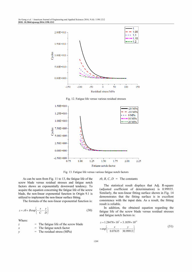
When the surface roughness of the screw blade is 12.5 µm, the fatigue life of the screw blade versus residual stresses and fatigue notch factors is shown in Fig. 11. According to Fig. 11, with the rise in residual stresses and fatigue notch factors, the fatigue life of the screw blade plummets. Evidently, the fatigue life of the screw blade is not a constant, which is a value varying with the manufacturing level of the screw blade. In addition, the line graph of the fatigue life versus various residual stresses and the curve diagram of the fatigue life versus various fatigue notch factors are shown in Fig. 12 and 13, respectively.

Fig. 11. Fatigue life versus residual stresses and fatigue notch factors


1209

Fig. 12. Fatigue life versus various residual stresses

Fig. 13. Fatigue life versus various fatigue notch factors

As can be seen from Fig. 11 to 13, the fatigue life of the screw blade versus residual stresses and fatigue notch factors shows an exponentially downward tendency. To acquire the equation concerning the fatigue life of the screw blade, the non-linear exponential function in Origin 9.1 is utilized to implement the non-linear surface fitting.

The formula of the non-linear exponential function is:

0 expx y

z z BC D

= + − −

(30)

Where: z = The fatigue life of the screw blade x = The fatigue notch factor y = The residual stress (MPa)

z0, B, C, D = The constants

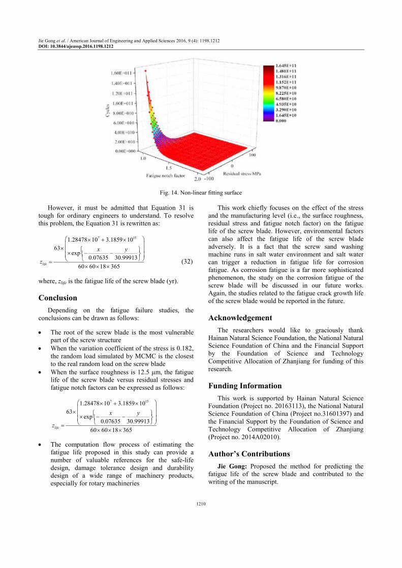
The statistical result displays that Adj. R-square (adjusted coefficient of determination) is 0.99935. Similarly, the non-linear fitting surface shown in Fig. 14 demonstrates that the fitting surface is in excellent consistence with the input data. As a result, the fitting result is reliable.

In addition, the obtained equation regarding the fatigue life of the screw blade versus residual stresses and fatigue notch factors is:

7 151.28478 10 3.1859 10

exp0.07635 30.99913

z

x y

= × + ×

× − −

(31)


1210

Fig. 14. Non-linear fitting surface

However, it must be admitted that Equation 31 is tough for ordinary engineers to understand. To resolve this problem, the Equation 31 is rewritten as:

7 151.28478 10 3.1859 10

63exp

0.07635 30.99913

60 60 18 365life

x y

z

× + × × × − − =

× × × (32)

where, zlife is the fatigue life of the screw blade (yr).

Conclusion

Depending on the fatigue failure studies, the conclusions can be drawn as follows: • The root of the screw blade is the most vulnerable

part of the screw structure • When the variation coefficient of the stress is 0.182,

the random load simulated by MCMC is the closest to the real random load on the screw blade

• When the surface roughness is 12.5 µm, the fatigue life of the screw blade versus residual stresses and fatigue notch factors can be expressed as follows:

7 151.28478 10 3.1859 10

63exp

0.07635 30.99913

60 60 18 365life

x y

z

× + × × × − − =

× × ×

• The computation flow process of estimating the

fatigue life proposed in this study can provide a number of valuable references for the safe-life design, damage tolerance design and durability design of a wide range of machinery products, especially for rotary machineries

This work chiefly focuses on the effect of the stress and the manufacturing level (i.e., the surface roughness, residual stress and fatigue notch factor) on the fatigue life of the screw blade. However, environmental factors can also affect the fatigue life of the screw blade adversely. It is a fact that the screw sand washing machine runs in salt water environment and salt water can trigger a reduction in fatigue life for corrosion fatigue. As corrosion fatigue is a far more sophisticated phenomenon, the study on the corrosion fatigue of the screw blade will be discussed in our future works. Again, the studies related to the fatigue crack growth life of the screw blade would be reported in the future.

Acknowledgement

The researchers would like to graciously thank Hainan Natural Science Foundation, the National Natural Science Foundation of China and the Financial Support by the Foundation of Science and Technology Competitive Allocation of Zhanjiang for funding of this research.

Funding Information

This work is supported by Hainan Natural Science Foundation (Project no. 20163113), the National Natural Science Foundation of China (Project no.31601397) and the Financial Support by the Foundation of Science and Technology Competitive Allocation of Zhanjiang (Project no. 2014A02010).

Author’s Contributions

Jie Gong: Proposed the method for predicting the fatigue life of the screw blade and contributed to the writing of the manuscript.


1211

Yun-Fei Fu: Organized the study and contributed to the writing of the manuscript.

Wen Xia: Designed the research plan. Ji-Hua Li: Contributed to the writing of the

manuscript. Fan Zhang: Compiled the MATLAB program of

NSGA-II.

Ethics

This article is original and contains unpublished material. The corresponding author confirms that all of the other authors have read and approved the manuscript and no ethical issues involved.

References

Baek, S.H., S.S. Cho and W.S. Joo, 2008. Fatigue life prediction based on the rainflow cycle counting method for the end beam of a freight car bogie. Int. J. Auto. Tech.-Kor., 9: 95-101.

DOI: 10.1007/s12239-008-0012-y Chen, S.M., T.Z. Shi, D.F. Wang and J. Chen, 2015.

Multi-objective optimization of the vehicle ride comfort based on kriging approximate model and NSGA-II. J. Mech. Sci. Technol., 29: 1007-1018. DOI: 10.1007/s12206-015-0215-x

Cheng, H.W., J.Y. Tao, X. Chen and Y. Jiang, 2014. Fatigue reliability evaluation of structural components under random loadings. P. I. Mech. Eng. O-J. Ris., 228: 469-477.

DOI: 10.1177/1748006X14527927 Cunha, S.B., I.P. Pasqualino and B.C. Pinheiro, 2009.

Stress-life fatigue assessment of pipelines with plain dents. Fatigue Fract. Eng. Mater. Struct., 32: 961-974. DOI: 10.1111/j.1460-2695.2009.01396.x

Fu, Y.F., J. Gong, Z. Peng, J.H. Li and S.D. Li et al., 2016. Optimization design for screw wash-sand machine based on fruit fly optimization algorithm. J. Applied Sci. Eng., 19: 149-161.

DOI: 10.6180/jase.2016.19.2.05 Fu, Y.F., J. Gong, Z.M. Yang, P.W. Li and S.D. Li et al.,

2015. Reliability analysis of mechanical sand washing system. Proceedings of the International Conference on Advances in Energy, Environment and Chemical Engineering, Sep. 26-27, Atlantis Press, France, pp: 533-536.

DOI: 10.2991/aeece-15.2015.107 Gholami, M.H. and M.R. Azizi, 2014. Constrained

grinding optimization for time, cost and surface roughness using NSGA-II. Int. J. Adv. Manuf. Tech., 73: 981-988.

DOI: 10.1007/s00170-014-5884-6 Harris, D. and T. Jur, 2009. Classical fatigue design

techniques as a failure analysis tool. J. Fail. Anal. Preven., 9: 81-87. DOI: 10.1007/s11668-008-9202-1

Johannesson, P., 2006. Extrapolation of load histories and spectra. Fatigue Fract. Eng. Mater. Struct., 29: 201-207. DOI: 10.1111/j.1460-2695.2006.00982.x

Johannesson, P. and J.J. Thomas, 2001. Extrapolation of rainflow matrices. Extremes, 4: 241-262.

DOI: 10.1023/A:1015277305308 Kan, R. and X.L. Wang, 2010. On the distribution of the

sample autocorrelation coefficients. J. Econometr., 154: 101-121. DOI: 10.1016/j.jeconom.2009.06.010

Lee, Y.L., J. Pan, R.B. Hathaway and M.E. Barkey, 2005. Fatigue Testing and Analysis: Theory and Practice. 1st Edn., Elsevier Butterworth-Heinemann, Oxford, ISBN-10: 9780750677196, pp: 15.

Mi, C.J., Z.Q. Gu, Y. Zhang, S.C. Liu and S. Zhang et al., 2016. Frame weight and anti-fatigue co-optimization of a mining dump truck based on Kriging approximation model. Eng. Fail. Anal., 66: 177-186. DOI: 10.1016/j.engfailanal.2016.03.021

Müller, G., 2009. Simplified theory of archimedean screws. J. Hydraul. Res., 47: 666-669.

DOI: 10.3826/jhr.2009.3475 Murugan, P., S. Kannan and S. Baskar, 2009. NSGA-II

algorithm for multi-objective generation expansion planning problem. Electr. Pow. Syst. Res., 79: 622-628. DOI: 10.1016/j.epsr.2008.09.011

Narayanan, G., K. Rezaei and U. Nackenhorst, 2016. Fatigue life estimation of aero engine mount structure using Monte Carlo simulation. Int. J. Fatigue, 83: 53-58.

DOI: 10.1016/j.ijfatigue.2015.03.030 Pezo, L., A. Jovanović, M. Pezo, R. Čolović and B.

Lončar, 2015. Modified screw conveyor-mixers-discrete element modeling approach. Adv. Powder Technol., 26: 1391-1399.

DOI: 10.1016/j.apt.2015.07.016 Robert, C.P. and G. Casella, 2004. Monte Carlo

Statistical Methods. 2nd Edn., Springer, New York, ISBN-10: 9780387212395, pp: 205.

Schijve, J., 2014. Fatigue of Structures and Materials. 2nd Edn., Aviation Industry Press, Beijing,

ISBN-10: 9787516504031, pp: 47. Shi, X.M., N. Xie, K. Fortune and J. Gong, 2012.

Durability of steel reinforced concrete in chloride environments: An overview. Constr. Build. Mater., 30: 125-138.

DOI: 10.1016/j.conbuildmat.2011.12.038 Tsai, Y.T. and K.S. Wang, 2015. A study of reliability

analysis of fatigue life for dental implants. J. Chin. Soc. Mech. Eng., 36: 439-448.

Vedalakshmi, R., R.R. Devi, B. Emmanuel and N. Palaniswamy, 2008. Determination of diffusion coefficient of chloride in concrete: An electrochemical impedance spectroscopic approach. Mater. Struct., 41: 1315-1326.

DOI: 10.1617/s11527-007-9330-1


1212

Vrugt, J.A., 2016. Markov chain Monte Carlo simulation using the DREAM software package: Theory, concepts and MATLAB implementation. Environ. Modell. Softw., 75: 273-316.

DOI: 10.1016/j.envsoft.2015.08.013 Wang, J.X., H.B. Chen, Y. Li, Y.Q. Wu and Y.S. Zhang,

2016. A review of the extrapolation method in load spectrum compiling. Stroj. Vestn. J. Mech. E., 62: 60-75. DOI: 10.5545/sv-jme.2015.2905

Wang, J.X., J.H. Zhang, Y.L. Liang and Y.H. Yang, 2012a. A cyclic simulation approach for the generation of the non-stationary load histories of engineering vehicles. J. Mech. Sci. Technol., 26: 1547-1554. DOI: 10.1007/s12206-012-0315-9

Wang, T.L., X.M. Guo, Q.E. Zhang and Y. Cai, 2012b. FEA and optimization design of screw of screw conveyor. Coal Mine Mach., 33: 14-16.

DOI: 10.13436/j.mkjx.2012.12.001 Wu, Y.Z., W.J. Li and Y.H. Liu, 2016. Fatigue life

prediction for boom structure of concrete pump truck. Eng. Fail. Anal., 60: 176-187.

DOI: 10.1016/j.engfailanal.2015.11.040 Xie, L.Y., 2013. Reliability Design. 1st Edn., Higher

Education Press, Beijing, ISBN-10: 9787040366761, pp: 11.

Yang, Z.M., S.D. Li, Y.F. Fu, M.Z. Lv and F. Zhang et al., 2016. Research on new desalination method of sea sand and its properties. Guangdong Chem. Ind., 43: 54-56. DOI: 10.3969/j.issn.1007-1865.2016.18.024

Zhang, Q.M., P. Wang, W.J. Wang and Y.X. Zhang, 2010. Marine sand resources in the Pearl River estuary waters of China. J. Marine Syst., 82: S83-S89. DOI: 10.1016/j.jmarsys.2010.02.007

Zheng, X.L. and J.F. Wei, 2005. On the prediction of P-

S-N curves of 45 steel notched elements and probability distribution of fatigue life under variable amplitude loading from tensile properties. Int. J. Fatigue, 27: 601-609.

DOI: 10.1016/j.ijfatigue.2005.01.001 Zhou, X.Y., Z.L. Hu, X.P. Qin, Y.J. Tao and L. Hua,

2016. Study on the stress characteristic and fatigue life of the shredder pin. Eng. Fail. Anal., 59: 444-455. DOI: 10.1016/j.engfailanal.2015.11.003

Zio, E., 2012. The Monte Carlo Simulation Method for System Reliability and Risk Analysis. 1st Edn., Springer, New York, ISBN-10: 9781447145875, pp: 127.

Fatigue Life Prediction of Screw Blade in Screw Sand...

Documents

Transcript of Fatigue Life Prediction of Screw Blade in Screw Sand...