Fatigue Life Prediction of Drill-String Subjected to ...

FATIGUE LIFE PREDICTION OF DRILL-STRING SUBJECTED TO RANDOMLOADINGS

Jiahao Zheng∗Faculty of Engineeringand Applied Science

Memorial University of NewfoundlandSt John’s, Newfoundland and Labrador, Canada A1B 3X5

Email: [email protected]

Hongyuan QiuFaculty of Engineeringand Applied Science



Jianming YangMember of ASME

Faculty of Engineering and Applied ScienceMemorial University of Newfoundland

St John’s, Newfoundland and Labrador, Canada A1B 3X5Email: [email protected]

Stephen ButtFaculty of Engineering and Applied Science



ABSTRACTBased on linear damage accumulation law, this paper in-

vestigates the fatigue problem of drill-strings in time domain.Rainflow algorithms are developed to count the stress cycles.The stress within the drill-string is calculated with finite elementmodels which is developed using Euler-Bernoulli beam theory.Both deterministic and random excitations to the drill-string sys-tem are taken into account. With this model, the stress timehistory in random nature at any location of the drill-string canbe obtained by solving the random dynamic model of the drill-string. Then the random time history is analyzed using rainflowcounting method. The fatigue life of the drill-string under bothdeterministic and random excitations can therefore be predicted.

NOMENCLATUREle Finite element length

∗Corresponding author.

g = 9.84 m/s2 Gravity AccelerationG = 7.6923∗1010 N/m2 Drill-string shear modulusE = 210 GPa Drill-string elastic modulusr = 7850 kg/m3 Drill-sting densityE0 = 4∗1010 N/m2 Rock elastic modulusν = 0.25 Poisson ratioG0 = 1.6∗1010 N/m2 Rock shear modulusr0 = 2100 kg/m3 Rock densitykc = 4.27∗109 N/m Rock stiffnessc = 1.05∗106 Rock damping coefficientm = 500kg Stabilizer masskst = 10 MN/m Stabilizer stiffnessr = 0.03 m Eccentric distance of stabilizer massw Average bit speedrb = 0.22 Bit radiusL = 0.005 H Motor inductanceRm = 0.01 W Armature resistanceKm = 6 V/s Motor inductance

1 Copyright © 2014 by ASME

Proceedings of the ASME 2014 International Mechanical Engineering Congress and Exposition IMECE2014

November 14-20, 2014, Montreal, Quebec, Canada

IMECE2014-36009

Figure 1: The simplified model of the system

n = 7.2 Gear ratio of the gearboxα = 0.01β = 0.01c1 = 1.35∗10−8 Coefficient of the ROP modelc2 =−1.8∗10−4 Coefficient of the ROP modelξ0 = 1 Coefficient of the TOB modelα1 = 2 Coefficient of the friction modelα2 = 1 Coefficient of the friction modela = 14.7 Coefficient of the S-N curveb1 =−3.46 Coefficient of the S-N curveb2 =−1.65∗10−5 Coefficient of the S-N curve

INTRODUCTIONIn drilling operations, fatigue is the main cause for most

of drill-string failures according to field data gathered over thepast few years [1]. Drill-string failures increase the cost ofdrilling dramatically. Although many studies have been con-ducted to address the fatigue failure problem, the frequency ofoccurrence of drill-string failure remains high. Thus, the avoid-ance of catastrophic drill-string failures caused by fatigue dam-age during drilling operations is of great economic significance.There are rich literatures on experimental works of fatigue fail-ure of drill-string. Among many experimental works, the fol-lowing three are most representative. Bachman [2] reported thetest result of full-size drill pipes from Hughes Tool Company. In

his test, the drill pipes were clamped as cantilevered beams andsubjected to rotational bending. The data obtained in this workformed the basis for the guideline in API RP7G. In this work,no axial load was considered, and the test was conducted in air.Morgan and Robin [3] tested small-scale coupons cut from as-produced seamless hot-rolled drill pipes. In this work, axial loadwas applied to the specimens. In 1991, Grondin and Kulak con-ducted their experiment using full-size drill pipes [4]. Their testsprovided the most comprehensive data for drill-string fatigue inwhich full-size drill pipes were subjected to axial load, fluctuat-ing bending and rotating bending in both air and corrosive media.The data provided by these experimental works formed the basisfor theoretical prediction of fatigue.

Also, several theoretical models are developed to analyze fa-tigue failures of drill-strings. Theoretical works on drill-stringfatigue have been developed mainly along two lines. One isbased on fracture mechanics theory [5]. This method assumesmicro cracks exist in the drill pipe materials. These micro crackspropagate in the drill pipe body along certain directions undercyclic loadings, and will eventually develop into fractures [6–8].The other method combines the traditional S-N curve and linearcumulative law based upon which the equivalent damage to thefatigue life of the drill pipe caused by cyclic loadings with dif-ferent amplitudes is calculated and summed [9–12]. This groupof method was initiated by Lubinski [9], and many modificationswere made to the S-N curves and boundary conditions by Hans-ford and Lubinski [10], Wu [11,12] and other researchers. Com-paratively, the second group of methods is more widely accepted,partly because it has more solid data supports from experimen-tal works. It is also reported that prediction made by the firstgroup of methods (fracture mechanics) is less conservative thanby the second (S-N curve plus linear cumulative fatigue dam-age) [6]. Although several models have been constructed to pre-dict drill-string fatigue, limitations still exist. First, all researchworks with exception of Patel and Vaz [13] dealt only with thecyclic loadings caused by dog-leg and/or drill-string buckling,without account for vibration which is a very important contribu-tor to fatigue of drill-strings. Secondly, Patel and Vaz’s work onlydealt with fatigue to drill-strings caused by deterministic cyclicstresses; therefore, it was unable to predict the fatigue caused byrandom stresses. However, it has long been recognized that thevibration of drill-strings is random in essence [14]. This fact re-quires that fatigue prediction of drill-string is better conductedwith random vibration theory. Aiming at this need, this paperdevelops a random dynamic model of drill-string with finite el-ement method (FEM). The random stresses within a drill-stringare calculated with the FEM model and the fatigue accumulationcaused by the random stress is investigated. The paper is orga-nized as follows. In section 2, the dynamic model used in thispaper is developed. Following that, mechanisms for the fatigueprediction used in this paper, including the cycle counting meth-ods and the S-N curves, are presented in section 3. Then simula-


Figure 2: Degrees of freedom of an element

tion results from deterministic and random cases are analyzed insection 4. Finally, conclusions are drawn in section 5.

DYNAMIC MODELPrimary Model

A typical rotary drilling system commonly seen in the oiland gas industry is illustrated in Fig. 1. This paper focuses onthe vibrations in axial and torsional directions. The drill-string isdiscretized using Lagrange linear shape function with axial andtorsional displacements. the axial displacement u and twistingangle θu of a element can be presented as:

u = Nuq, θu = Nθq (1)

where Nu, and Nθ are shape function matrices, and q is the vectorof nodal coordinates of the two-node finite element as shown inFig. 2, which is defined by:

q = {u1 θu1 u2 θu2}T (2)

where u, represents x− translational degree of freedom (DOF),while θu represents the rotational DOF around the x− axe.

By defining the element length le and the non-dimensionalelement variable ξ = x/le, the shape function matrices are givenas:

N1 = 1−ξ (3)N2 = ξ (4)

Nu = {N1,0,N2,0} (5)Nθ = {0,N1,0,N2} (6)

The expression for the linear stiffness Ke is:

Ke =∫ 1

0[EAle

N′Tu N

′u +

GJle

N′Tθ N

′θ]dξ (7)

where Nu and Nθ are for axial and torsional respectively. Theexpression for the mass matrix Me is:

Me =∫ 1

0[ρAleNT

u Nu +ρJleNTθ Nθ]dξ (8)

Substituting Eqn. (3) through (6) into Eqn. (7) and (8), the linearstiffness Ke and mass Me are obtained:

Ke =

EAle 0 −EA

le 00 GJ

le 0 −GJle

−EAle 0 EA

le 00 −GJ

le 0 GJle

(9)

Me =

ρAle

3 0 ρAle6 0

0 ρJle3 0 ρJle

6ρAle

6 0 ρAle3 0

0 ρJle6 0 ρJle

3

(10)

By assembling the local stiffness and mass matrices, the system’sglobal mass and stiffness matrices can be obtained. In the cur-rent paper, the drill-string is divided into 30 elements: 20 fordrill-pipe section and 10 for drill-collar section. Considering theboundary conditions, the drill-string finite element model con-tains 62 DOF in total.

After cer mathematical manipulations and taking the mass ofthe stabilizer into account, the equations of motion for the systemcan be represented in a compact matrix form as:

Mq(t)+Cq(t)+Kq(t) = F(x, x,φ, φ,Fc, I) (11)

M = M′+Am (12)

where M′, C and K are system global mass, damping andstiffness matrices, respectively, q(t) is the displacement vector,F(x, x,φ, φ,Fc, I) is the excitation vector which is random in na-ture including WOB, TOB, Fg, Fh and Trb. A is the correspond-ing transformation matrices, while m is the mass of the stabilizerwhich is assumed to be 500 kg in this paper.The downhole damping C is assumed to be a linear combinationof K and M as below:

C = αM+βK (13)


where α and β are constants to be selected. In this paper the sys-tem is assumed as underdamped which is common in engineeringapplication.

Deterministic Excitations WOB, the weight on bit, isrepresented as:

WOB =

{kc(x− s)+ c(x− s) x≥ s

0 x < s (14)

where x is the displacement of the bit, kc is the formation contactstiffness, c is the rock damping coefficient and s is the elevationof the formation surface. kc , c and s can be computed by [15,16]

G0 =E0

2(1+ν)(15)

kc =G0r0

1−ν(16)

c =3.4r2

0√

G0ρ0

1−ν(17)

s = s0sin(φ) (18)

where E0, G0, ν, ρ0 are determined by the property of the rock,r0 is the foundation diameter, φ is bit torsional displacement.The torque on bit (TOB) is related with WOB and cutting condi-tions [15], and can be calculated by:

TOB =WOBrb(µ(φ)+ξ0

√δc

rb) (19)

where rb is the radius of the bit and δc is the depth of cut percircle:

δc =2πROP

w(20)

ROP, representing the average rate of penetration, is given as[15]:

ROP = c1F0√

w+ c2 (21)

where F0 is the difference between the total weight and the hookload, w is the average bit speed. µ(φ) is modeled as a continuousfunction [15]:

µ(φ) = µ0(tanh φ+α1φ

1+α2φ2+νφ) (22)

Fg is the elementary load vector resulting from the gravity field:

Fg =∫ 1

0ρgAleNT

u dξ+Cmg (23)

where C is the corresponding transformation matrix.Fh is the hook load given as:

Fh = rcWr (24)

where rc is a constant ratio, Wr is the total weight of the drillingsystem. In this paper, the weight of drill-pipe is about 43 percentof the total weight. In order to make the drill-pipe under tensionand put the central point in drill-collar part, rc is chosen to belarger than 0.5 in the simulations.Trb is the torque given by the rotary table. It is assumed in thispaper that the rotary table is driven by a DC motor through a gearbox and Trb is given as [15]:

LI +RmI +Kmnφrt =Vc (25)Vc = Kmnwd (26)Trb = KmnI (27)

where I is the motor current and φrt is the speed of the rotarytable. wd is assumed to be the desired table speed in this paper.

Random Components Considering the randomness ofthe downhole excitation, two stationary Gaussian white noiseW1(t) and W2(t) are introduced into the bit axial and torsional di-rections as the random components. The continuous time whitenoise excitation needs to be discretized in the simulation. It isachieved by using [17]:

W (ti) =

√2πS0

∆tUi (28)

where random variables Ui are normal distributed with zero meanand unit standard deviation and time step ∆t depends on the max-imum natural frequency ωn of the system. ∆t is determined bythe following equation:

∆t <2π

ωn× 1

10(29)

Therefore, the equation of motion for the system is renewed as:

Mq(t)+Cq(t)+Kq(t)=F(x, x,φ, φ,Fc, I)+T1 ·W1(t)+T2 ·W2(t)(30)


where T1 and T2 are transformation matrices, which will putW1(t) and W2(t) into bit axial and torsional directions respec-tively.

Solution Strategy The equation of motion for the sys-tem is given as:

Mq(t)+Cq(t)+Kq(t) = F (31)

where F is the excitation vector including deterministic and ran-dom components. Eqn. (31) is valid for any given time instant qi.Using the central difference method, the acceleration and veloc-ity vectors at time ti can be written as [18]:

qi =1

2∆t(qi+1−qi−1) (32)

qi =1

∆t2 (qi+1−2qi +qi−1) (33)

By substituting Eqns. (32) and (33) into Eqn. (31), and rearrang-ing the terms one has [18]:

qi+1 = ∆t2N1Fi +N2qi +N3qi−1 (34)

with

N1 = [M+12

∆tC]−1 (35)

N2 = N1[2M−∆t2K] (36)

N3 = N1[12

∆tC−M] (37)

M, K, C are all constants at each time step. However, Eqn. (32)can not be used directly here to calculate qi because the value ofqi+1 is unknown. To solve this problem, velocity vectors at timeti are calculated in terms of:

qi = qi−1 + qi−1∆t (38)

with

qi−1 = M−1[Fi−1−Cqi−1−Kqi−1] (39)

The torque given by the DC motor f (Ii) is given as:

f (Ii) = Trbi = KmnIi (40)

Ii =1L× (2∆tVc−2∆tnKmφi−1−2RmIi−1∆t +LIi−2) (41)

Figure 3: Random stress time history of the bottom (30th ele-ment) of the drill-string (time interval: 120s, 10s respectively)

Once the displacement vector at each time step is obtained, theaxial stress σu and torsional stress τ for each element are com-puted as:

σu = E∆ule

(42)

τ = GD∆φ

2le(43)

where E and G are elasticity and shear modulus of the drill-string, D is the outer diameter, ∆u and ∆φ are the axial and tor-sional relative displacements between the two nodes of each el-ement. It should be noted that the largest torsional shear stress τ

is at the outer surface of the drill-string. The stress finally usedfor fatigue calculation in the following sections is the maximumprincipal stress σp, which is calculated from:

σ3p−σuσ

2p− τσp +σuτ

2 = 0 (44)

FATIGUE DAMAGE AND LIFE PREDICTIONBy solving the dynamic model of Eqn. (11), the displace-

ments along with the stress values within the drill-string can beobtained under specific excitations. An example of a stress timehistory of the 30th element (at the bottom of the drill-string) isshown in Fig. 3. The the stress data X(t) is saved in an [n× 2]matrix in which the first column represents the discretized timeinstants and the second represents the corresponding stress val-ues. This stress matrix is the basis of fatigue calculations in thefollowing section. The procedures for the fatigue calculation areillustrated in the flowchart shown in Fig. 4.


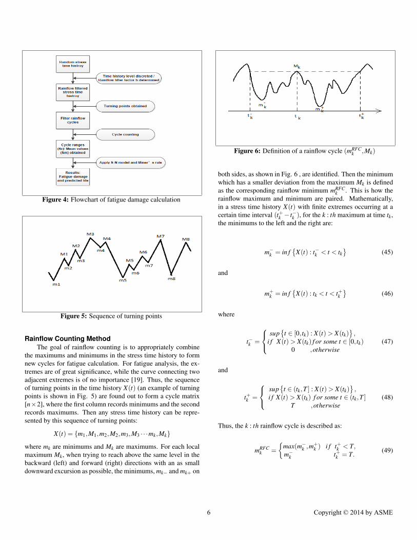
Figure 4: Flowchart of fatigue damage calculation

Figure 5: Sequence of turning points

Rainflow Counting MethodThe goal of rainflow counting is to appropriately combine

the maximums and minimums in the stress time history to formnew cycles for fatigue calculation. For fatigue analysis, the ex-tremes are of great significance, while the curve connecting twoadjacent extremes is of no importance [19]. Thus, the sequenceof turning points in the time history X(t) (an example of turningpoints is shown in Fig. 5) are found out to form a cycle matrix[n×2], where the first column records minimums and the secondrecords maximums. Then any stress time history can be repre-sented by this sequence of turning points:

X(t) = {m1,M1,m2,M2,m3,M3 · · ·mk,Mk}

where mk are minimums and Mk are maximums. For each localmaximum Mk, when trying to reach above the same level in thebackward (left) and forward (right) directions with an as smalldownward excursion as possible, the minimums, mk− and mk+ on

Figure 6: Definition of a rainflow cycle (mRFCk ,Mk)

both sides, as shown in Fig. 6 , are identified. Then the minimumwhich has a smaller deviation from the maximum Mk is definedas the corresponding rainflow minimum mRFC

k . This is how therainflow maximum and minimum are paired. Mathematically,in a stress time history X(t) with finite extremes occurring at acertain time interval (t+k − t−k ), for the k : th maximum at time tk,the minimums to the left and the right are:

m−k = in f{

X(t) : t−k < t < tk}

(45)

and

m+k = in f

{X(t) : tk < t < t+k

}(46)

where

t−k =

sup{

t ∈ [0, tk) : X(t)> X(tk)},

i f X(t)> X(tk) f or some t ∈ [0, tk)0 ,otherwise

(47)

and

t+k =

sup{

t ∈ (tk,T ] : X(t)> X(tk)},

i f X(t)> X(tk) f or some t ∈ (tk,T ]T ,otherwise

(48)

Thus, the k : th rainflow cycle is described as:

mRFCk =

{max(m−k ,m

+k ) i f t+k < T,

m−k t+k = T. (49)


Figure 7: Stress cycle range and mean value

Defining mRFC(t) by Eqn. (49) as the rainflow minimum forall time t of the time history X(t), if x(t) is not a strict localmaximum of the time history, the rainflow range x(t)−mRFC(t)is set to be zero.

Finally, the rainflow cycles are obtained by the counting pro-gram and saved in a matrix of [n× 2], denoted by MRFC wherethe first column MRFC(:,1) records minimums and the secondcolumn MRFC(:,2) records maximums. The stress ranges (Sr)and mean stress (Sm) of each cycle are calculated using the fol-lowing equations as shown in Fig. 7.

Sr =∣∣MRFC(:,1)−MRFC(:,2)

∣∣ (50)

Sm =∣∣MRFC(:,1)+MRFC(:,2)

∣∣/2 (51)

Rainflow Filter Given the fact that very small cycleshave no significant impact on fatigue damage, but cause greatinconvenience to cycle counting, the stress data is filtered duringthe stress cycles are counted. This is achieved by setting a pre-determined threshold h [19, 20]. The rainflow filter will extractsall rainflow cycles (mRFC(t), x(t)) such that x(t)−mRFC(t)> h,while the cycle with ranges smaller than h are all removed.

An comparison between an original stress time history andits counterpart after the filter is given in Fig. 8. This stress iscalculated with h = 0.2 at the bottom (30th position) of the drill-string. From the comparison, it can be found that the small os-cillations in the original data are removed. To better illustratethe effect of the filter, histograms of the stress ranges before andafter the filter are given in Fig. 9, where the x-axis stands forstress range levels and the y-axis stands for the number of cy-cles counted. It can be clearly seen from part (a), that cycleswith small stress ranges are dominant. The ranges bigger than0.5× 107 Pa cannot be recognized though they exist. However,in part (b) where the stress ranges smaller than 1× 107 Pa hasbeen filtered, the bigger cycles counted stand out.

Figure 8: Original data and rainflow filtered data (when h = 0.2)

Figure 9: Comparison between original data and filtered data

S-N Model and Miner’s RuleS-N Model The model from Grondin and Kulak [4] ex-

pressed as Eqn. (52) is used to model the S-N curve of drill pipesin this paper.

log10[N(Sr,Sm)] = a+b1× log10(Sr)+b2× (Sm)2 (52)

where a,b1 and b2 are constant and they are taken the follow-ing values. a = 14.8, b1 = −3.46, b2 = −1.65× 10−5. Severalcurves with different mean stresses are shown in Fig. 10.


Figure 10: S-N model (Parameters: Sr, Sm)

Damage Accumulation The Palmgren-Miner lineardamage hypothesis is employed in this paper to model the dam-age caused by a specific stress as below.

k

∑i=1

ni

Ni=C (53)

where C is a constant which equals to 1 theoretically. In reality,it can be determined by experiment and is generally between 0.7and 2.2 [21]. The total damage is given by:

Dtotal =k

∑i=1

1Ni

(54)

where k is the total number of cycles counted from the randomtime history and Ni is the corresponding cycles until failure ofthe ith cycle. Then the predicted life is given by:

Tpredicted =1

Dβ

(55)

Dβ =Dtotal

l(56)

where Dβ is the damage intensity, i.e. how much damage is ac-cumulated per unit time. l is the length of the stress time historybeing analyzed.

RESULTS ANALYSISFatigue Analysis Under Deterministic Excitation

By setting the random component of the excitations to zero,the fatigue under deterministic excitations can be examined. Fig.12 shows the predicted life of the drill-string from the top (El-ement No.1) to the bottom (Element No.30), under certain de-terministic excitations. Simulation results with the rotary speedωd = 15 rad/s, ωd = 30 rad/s and ωd = 45 rad/s, are givenin three sub-figures.

One observation made on those figures is that the fa-tigue damage at ωd = 15 rad/s is much bigger than that atωd = 30 rad/s and ωd = 45 rad/s. This seems contradictorywith common sense. However, the existence of stick-slip phe-nomenon observed in the field makes this reasonable. Also, afterexamination of the dynamic response, which is not given herefor the sake of space-saving, it is found that at ωd = 15 rad/sstick-slip does happens to the system. Therefore, the damage tothe fatigue is much severe in this case of slower rotary speed.Once the rotation speeds up, stick-slip will be reduced whichmakes the damage to fatigue decreases. This is verified with thatat ωd = 45 rad/s the life prediction values are generally biggerthan the counterpart at ωd = 30 rad/s except several positions.

Another observation is that the position has different fa-tigue damage. This is resulted from the diverse values of stressranges and mean stress. From Fig. 12, it can be seen thatat ωd = 15 rad/s the damage decreases with the increase ofdepth. However, this trend is not observed with ωd = 30 rad/sand ωd = 45 rad/s. In order to find the reason for this, thestress time histories for different positions with the same rotaryspeed ωd = 30 rad/s are examined and depicted on Fig. 11. Itcan be seen that with increase of depth the ranges of stress be-come larger. Bigger cycle range means severer fatigue damageto the drill-string. However, at deeper position, the mean stress islower. This is easy to understand because the drill-collar part isusually in compression with mean stress values negative. Whilein the drill-pipe part mean stress values are positive because ofbeing in tension. The mean stress changes sign at the neutralpoint between element No. 23 and 24, which can be seen thefigure. Life prediction of this set of stress time histories is shownas the second plot in Fig. 12. No obvious life prediction chang-ing pattern is found in this plot, which explains that the fatiguedamage comes from two conflicting factors: the mean and therange.

Fatigue Analysis of Random ResultsBy assuming the intensity of W1(t) and W2(t) as 100, the ef-

fect of random excitations are examined. The predicted life inthis case at ωd = 15, 30, 45 rad/s are presented in Fig. 13 withthe same deterministic loads with the previous case. Changes oflife prediction values can be observed between Fig. 12 and 13,while the basic shape of the curves does not change. This maybe


Figure 11: Stress time histories of drill-string when wd = 30 rad/s

because the effect of the random component is minor comparedwith the deterministic part. Due to the lack of knowledge aboutthe intensity and the spectral characteristic of the random load-ings, no further work is done at this point for this random effect.However, with more knowledge of the random part, there will beno theoretical difficulty in digging deeper into this topic. Thiswill be reported in future publications.

CONCLUSIONSThis paper develops a fatigue prediction methodology to

drill-strings based on linear accumulation law and rainflow cy-cle counting method. The model accounts for the stress causedby drill-string vibrations, including both deterministic vibrationand random vibration. The dynamic stress at different positionof the drill-string is obtained through solving a FEA dynamicmodel. The following conclusions are drawn from this paper.

1. Stick-slip phenomenon has severer negative effect on the fa-tigue life of drill-string. It should be avoided in drilling op-eration.

2. Under non-stick-slip condition, the fatigue life increases

with the increase of rotary speed. This is because the drill-string tends to operate more smoothly with a larger rotaryspeed.

3. The different life predictions at different position of the drill-string are affected by two factors: mean stress and stressrange. Depending on different operational conditions, dif-ferent critical point of the drill-string may be found.

4. The random excitations have obvious effect on the fatiguelife of drill-string. The amount of the effect depends on theintensity and the spectral characteristic of the random exci-tations.

ACKNOWLEDGMENT

This work is sponsored financially by Research & Develop-ment Corporation of Newfoundland and Labrador, Canada, un-der an Ignit R & D Grant. The authors would like to thank thesponsor for their support.


Figure 12: Predicted life of the drill-string (Under deterministic excitations)

REFERENCES[1] Baryshnikov, A., Calderoni, A., Ligrone, A., and Ferrara,

P., 1997. “A new approach to the analysis of drillstringfatigue behaviour”. SPE Drilling & Completion, 12(2),pp. 77–84.

[2] Bachman, W., 1951. “Fatigue testing and development ofdrill pipe to tool joint connection”. World Oil, 132, p. 104.

[3] Morgan, R. P., and Robin, M. J., 1969. “A method for theinvestigation of fatigue strength in seamless drillpipe”.

[4] Grondin, G. Y., and Kulak, GL, U. o. A. D. o. C. E., 1991.Fatigue of drill pipe. Department of Civil Engineering,University of Alberta.

[5] Sobczyk, K., and Spencer Jr, B., 1992. Random fatigue:from data to theory. Access Online via Elsevier.

[6] Vaisberg, O., Vincke, O., Perrin, G., Sarda, J., and Fay, J.,2002. “Fatigue of drillstring: state of the art”. Oil & GasScience and Technology, 57(1), pp. 7–37.

[7] Sikal, A., Boulet, J., Menand, S., and Sellami, H., 2008.“Drillpipe stress distribution and cumulative fatigue analy-sis in complex well drilling: New approach in fatigue opti-mization”. In SPE Annual Technical Conference and Exhi-bition.

[8] PE, T., Sean, E., PhD, K., Nicholas, R., and Nanjiu, Z.,2004. “An innovative design approach to reduce drill string

fatigue”. In IADC/SPE Drilling Conference.[9] Lubinski, A., 1961. “Maximum permissible dog-legs in

rotary boreholes”. Journal of Petroleum Technology, 13(2),pp. 175–194.

[10] Hansford, J. E., and Lubinski, A., 1966. “Cumulativefatigue damage of drill pipe in dog-legs”. Journal ofPetroleum Technology, 18(3), pp. 359–363.

[11] Wu, J., 1996. “Drill-pipe bending and fatigue in rotarydrilling of horizontal wells”. In SPE Eastern RegionalMeeting.

[12] Wu, J., 1997. “Model predicts drill pipe fatigue in horizon-tal wells”. Oil and Gas Journal, 95(5).

[13] Patel, M., and Vaz, M., 1995. “Comparisons of drill stringcyclic loading due to vibration and dog-legs”. Proceedingsof the Institution of Mechanical Engineers, Part E: Journalof Process Mechanical Engineering, 209(1), pp. 17–25.

[14] Dareing, D. W., 2012. Mechanics of Drillstrings and Ma-rine Risers. ASME Press, New York, NY.

[15] Yigit, A. S., C. A. P., 2006. “Stick-slip and bit-bounce inter-action in oil-well drillstrings”. Journal of Energy ResourcesTechnology, 128, May, pp. 268–274.

[16] Gazetas, G., 1983. “Analysis of machine foundation vibra-tions: state of the art”. International Journal of Soil Dy-namics and Earthquake Engineering, 2(1), May, pp. 2–42.


Figure 13: Predicted life of the drill-string (Under random excitations)

[17] Bucher, C., 2009. Computational Analysis of Random-ness in Structural Mechanics: Structures and Infrastruc-tures Book Series. CRC Press.

[18] To, C., and Liu, M., 2000. “Large nonstationary randomresponses of shell structures with geometrical and mate-rial nonlinearities”. Finite elements in analysis and design,35(1), pp. 59–77.

[19] Brodtkorb, P. A., Johannesson, P., Lindgren, G., Rychlik, I.,Ryden, J., and Sjo, E., 2000. “Wafo–a matlab toolbox foranalysis of random waves and loads”. In Proceedings ofthe 10th international offshore and polar engineering con-ference, Vol. 3, pp. 343–350.

[20] Rychlik, I., 1996. “Simulation of load sequences from rain-flow matrices: Markov method”. International journal offatigue, 18(7), pp. 429–438.

[21] Schijve, J., 2001. Fatigue of structures and materials.Springer.


Fatigue Life Prediction of Drill-String Subjected to ...

Documents

Transcript of Fatigue Life Prediction of Drill-String Subjected to ...