FATIGUE ASSESSMENT OF OFFSHORE STRUCTURES › content › dam › eagle › rules-and... · •...
61
Guide for the Fatigue Assessment of Offshore Structures GUIDE FOR FATIGUE ASSESSMENT OF OFFSHORE STRUCTURES JUNE 2020 American Bureau of Shipping Incorporated by Act of Legislature of the State of New York 1862 2020 American Bureau of Shipping. All rights reserved. 1701 City Plaza Drive Spring, TX 77389 USA
Transcript of FATIGUE ASSESSMENT OF OFFSHORE STRUCTURES › content › dam › eagle › rules-and... · •...

G u i d e f o r t h e F a t i g u e A s s e s s m e n t o f O f f s h o r e S t r u c t u r e s
GUIDE FOR
FATIGUE ASSESSMENT OF OFFSHORE STRUCTURES
JUNE 2020
American Bureau of Shipping Incorporated by Act of Legislature of the State of New York 1862
2020 American Bureau of Shipping. All rights reserved. 1701 City Plaza Drive Spring, TX 77389 USA

ii ABS GUIDE FOR THE FATIGUE ASSESSMENT OF OFFSHORE STRUCTURES . 2020
F o r e w o r d
Foreword (1 June 2020) The main purpose of this Guide is to supplement the Rules and the other design and analysis criteria that ABS has issued for the Classification of some types of offshore structures. The specific Rules and other Classification criteria that are being supplemented by this Guide include the latest versions of the following documents:
• Rules for Building and Classing Offshore Installations
• Rules for Building and Classing Mobile Offshore Units
• Rules for Building and Classing Single Point Moorings
• Rules for Building and Classing Floating Production Installations
(However, the fatigue assessment of Ship-Type Floating Installations is to be performed in accordance with the FPI Rules, and not this Guide)
While some of the criteria contained herein may be applicable to ship structures, it is not intended that this Guide be used in the Classification of ships.
The June 2020 update of this Guide includes:
• Updated ABS S-N curves for tubular joints
• Updated FEA stress extrapolation procedure
• New section for post-weld improvement
• New section for new design S-N curves based on fatigue test data
• Updated time domain analysis method
• Updated fatigue strength based on fracture mechanics
• Updated formula for eccentricity SCF on double-sided plate butt welds
• Updated the section of existing structures
This Guide becomes effective on the first day of the month of publication.
Users are advised to check periodically on the ABS website www.eagle.org to verify that this version of this Guide is the most current.
We welcome your feedback. Comments or suggestions can be sent electronically to [email protected].

ABS GUIDE FOR THE FATIGUE ASSESSMENT OF OFFSHORE STRUCTURES . 2020 iii
T a b l e o f C o n t e n t s
GUIDE FOR
FATIGUE ASSESSMENT OF OFFSHORE STRUCTURES CONTENTS SECTION 1 Introduction .............................................................................................. 1
1 Terminology and Basic Approaches Used in Fatigue Assessment .... 1 1.1 General............................................................................................ 1 1.3 S-N Approach .................................................................................. 2 1.5 Fracture Mechanics ......................................................................... 2 1.7 Structural Detail Types .................................................................... 2 1.9 Alternative Criteria ........................................................................... 2
3 Damage Accumulation Rule and Fatigue Safety Checks ................... 3 3.1 General............................................................................................ 3 3.3 Definitions ........................................................................................ 3 3.5 Fatigue Safety Check ...................................................................... 3
5 Existing Structures .............................................................................. 4 7 Summary ............................................................................................. 4 FIGURE 1 Schematic of Fatigue Assessment Process (For each
location or structural detail) ....................................................... 4 SECTION 2 Fatigue Strength Based on S-N Curves ................................................ 5
1 Introduction ......................................................................................... 5 1.1 General............................................................................................ 5 1.3 Defining Parameters ........................................................................ 5 1.5 Tolerances and Alignments ............................................................. 5
3 Nominal Stress Method ....................................................................... 5 3.1 ‘Reference’ Stress and Stress Concentration Factor ....................... 5
5 Hot Spot Stress Method ...................................................................... 7 5.1 Non-Tubular Joints .......................................................................... 7 5.3 Tubular Joints .................................................................................. 7 5.5 Stress Definitions and Related Approaches .................................... 8 5.7 Finite Element Analysis to Obtain Hot Spot Stress .......................... 9 5.9 FEA Data Interpretation – Stress Extrapolation Procedure and
S-N Curves ...................................................................................... 9 7 Post-Weld Improvement ................................................................... 11
7.1 General.......................................................................................... 11 7.3 Weld Profiling by Machining or Grinding........................................ 12 7.5 Burr Grinding ................................................................................. 13 7.7 TIG Dressing ................................................................................. 14

iv ABS GUIDE FOR THE FATIGUE ASSESSMENT OF OFFSHORE STRUCTURES . 2020
7.9 Peening Method............................................................................. 15 7.11 Improvement of Fatigue Life .......................................................... 15
FIGURE 1 Two-Segment S-N Curve .......................................................... 7 FIGURE 2 Stress Gradients (Actual & Idealized) Near a Weld .................. 8 FIGURE 3 Location of the Hot Spot for Shell Models .............................. 10 FIGURE 4 Extrapolation of Stresses for Shell Finite Element Models ..... 11 FIGURE 5 Details of Weld Profiling .......................................................... 13 FIGURE 6 Details of Ground Weld Toe Geometry ................................... 14 FIGURE 7 Extent of Weld Toe Burr Grinding to Remove Inter-bead
Toes on Weld Face ................................................................. 14 SECTION 3 S-N Curves .............................................................................................. 16
1 Introduction ....................................................................................... 16 3 S-N Curves and Adjustments for Non-Tubular Details
(Specification of the Nominal Fatigue Strength Criteria) .................. 16 3.1 ABS Offshore S-N Curves ............................................................. 16
5 S-N Curves for Tubular Joints ........................................................... 21 5.1 ABS Offshore S-N Curves ............................................................. 21 5.3 Parametric Equations for Stress Concentration Factors ................ 22
7 Cast Steel Components .................................................................... 22 9 New Design S-N Curves Based on Fatigue Test Data ..................... 23
9.1 General .......................................................................................... 23 9.3 Fatigue Tests ................................................................................. 24 9.5 Statistical Analysis of Fatigue Test Data ........................................ 24
TABLE 1 Parameters for ABS-(A) Offshore S-N Curves for
Non-Tubular Details in Air ....................................................... 18 TABLE 2 Parameters for ABS-(CP) Offshore S-N Curves for
Non-Tubular Details in Seawater with Cathodic Protection ................................................................................ 19
TABLE 3 Parameters for ABS-(FC) Offshore S-N Curves for Non-Tubular Details in Seawater for Free Corrosion .............. 20
TABLE 4 Parameters for Class ‘T’ ABS Offshore S-N Curves ............... 22 TABLE 5 Parameters for ABS Offshore S-N Curve for Cast Steel
Joints (in-air) ........................................................................... 23 TABLE 6 Coefficient k* ........................................................................... 25 FIGURE 1 ABS-(A) Offshore S-N Curves for Non-Tubular Details in
Air ............................................................................................ 18 FIGURE 2 ABS-(CP) Offshore S-N Curves for Non-Tubular Details in
Seawater with Cathodic Protection ......................................... 19 FIGURE 3 ABS-(FC) Offshore S-N Curves for Non-Tubular Details in
Seawater for Free Corrosion ................................................... 20 FIGURE 4 ABS Offshore S-N Curves for Tubular Joints (in air, in
seawater with cathodic protection and in seawater for free corrosion) ......................................................................... 22
FIGURE 5 ABS Offshore S-N Curve for Cast Steel Joints (in-air) ........... 23

ABS GUIDE FOR THE FATIGUE ASSESSMENT OF OFFSHORE STRUCTURES . 2020 v
SECTION 4 Fatigue Design Factors ......................................................................... 26 1 General ............................................................................................. 26
SECTION 5 Simplified Fatigue Assessment Method .............................................. 27
1 Introduction ....................................................................................... 27 3 Mathematical Development .............................................................. 27
3.1 General Assumptions .................................................................... 27 3.3 Parameters in the Weibull Distribution .......................................... 27 3.5 Fatigue Damage for Single Segment S-N Curve ........................... 28 3.7 Fatigue Damage for Two Segment S-N Curve .............................. 28 3.9 Allowable Stress Range ................................................................ 29 3.11 Fatigue Safety Check .................................................................... 29
5 Application to Jacket Type Fixed Offshore Installations ................... 29 SECTION 6 Spectral-based Fatigue Assessment Method ..................................... 30
1 General ............................................................................................. 30 3 Floating Offshore Installations .......................................................... 30 5 Jacket Type Fixed Platform Installations .......................................... 30 7 Spectral-based Assessment for Floating Offshore Installations ....... 30
7.1 General.......................................................................................... 30 7.3 Stress Range Transfer Function .................................................... 31 7.5 Outline of a Closed Form Spectral-based Fatigue Analysis
Procedure ...................................................................................... 31
FIGURE 1 Spreading Angles Definition .................................................... 32
SECTION 7 Time Domain Analysis Method ............................................................. 36
1 General ............................................................................................. 36 3 Considerations for Time-Domain Analysis ........................................ 37
3.1 Time Step of the Simulations ......................................................... 37 3.3 Transient Responses .................................................................... 37 3.5 Relative Velocity ............................................................................ 37
5 Rainflow Cycle Counting ................................................................... 37 7 Damage Calculation from Rainflow Cycle Counting ......................... 38 FIGURE 1 Flowchart of Time-Domain Fatigue Analysis Method ............. 36 FIGURE 2 Segment of Stress Process to Demonstrate Rainflow
Cycle Counting Method ........................................................... 37 SECTION 8 Deterministic Method of Fatigue Assessment.................................... 39
1 General ............................................................................................. 39

vi ABS GUIDE FOR THE FATIGUE ASSESSMENT OF OFFSHORE STRUCTURES . 2020
SECTION 9 Fatigue Strength Based on Fracture Mechanics ................................ 40 1 Introduction ....................................................................................... 40 3 Crack Growth Model ......................................................................... 40
3.1 General Comments ........................................................................ 40 3.3 Crack Models ................................................................................. 40 3.5 The Paris Law ................................................................................ 41 3.7 Stress Intensity Factor Range ....................................................... 41
5 Life Prediction ................................................................................... 42 5.1 Number of Cycles and Crack Size ................................................. 42 5.3 Values of C and m .......................................................................... 43 5.5 Determination of Initial Flaw Size................................................... 43
7 Failure Assessment Diagram ............................................................ 43 7.1 General .......................................................................................... 43 7.3 Assessment Approaches ............................................................... 44 7.5 Material Properties ......................................................................... 45
9 Crack Interaction ............................................................................... 45 FIGURE 1 Definition of Crack Dimensions ............................................... 42 FIGURE 2 Failure Assessment Diagram (FAD) ....................................... 44
APPENDIX 1 Guidance on Structural Detail Classifications for Use with ABS
Offshore S-N Curves .............................................................................. 46 APPENDIX 2 References on Parametric Equations for the SCFs of Tubular
Intersection Joints .................................................................................. 53 1 Simple Joints ..................................................................................... 53 3 Multi Planar Joints ............................................................................. 53 5 Overlapped Joints ............................................................................. 53 7 Stiffened Joints ................................................................................. 53 9 References ........................................................................................ 55 TABLE 1 SCF Matrix Tables for X, K and T/Y Joints ............................. 54

ABS GUIDE FOR THE FATIGUE ASSESSMENT OF OFFSHORE STRUCTURES . 2020 1
S e c t i o n 1 : I n t r o d u c t i o n
S E C T I O N 1 Introduction
1 Terminology and Basic Approaches Used in Fatigue Assessment
1.1 General (1 June 2020) Fatigue assessment* is a process where the fatigue demand on a structural element is established and compared to the predicted fatigue strength of that element. One way to categorize a fatigue assessment technique is to say that it is based on a direct calculation of fatigue damage or expected fatigue life. Three important methods of assessment are the Simplified Method, the Spectral Method and the Deterministic Method. Alternatively, an indirect fatigue assessment may be performed by the Simplified Method, based on limiting a predicted (probabilistically defined) stress range to be at or below a permissible stress range. There are also assessment techniques that are based on Time Domain analysis methods that are especially useful for structural systems that are subjected to non-linear structural response or non-linear loading. * Note: ITALICS are used throughout the text to highlight some words and phrases. This is done solely to emphasize or
define terminology that is used in the presentation.
Fatigue Demand is stated in terms of stress ranges that are produced by the variable loads imposed on the structure. (A stress range is the absolute sum of stress amplitudes on either side of a ‘steady state’ mean stress. The term ‘variable load’ may be used in place of ‘cyclic load’ since the latter may be taken to imply a uniform frequency content of the load, which may not be the case.) Fatigue-inducing loads are the result of actions producing variable load effects. Most commonly for ocean-based structures, the biggest influences producing the higher magnitude variable loadings are waves and combinations of waves with other variables such as ocean current, and equipment-induced variable loads. Since the loads considered vary over time, it is possible that they could excite dynamic responses in the structure; this will amplify the acting fatigue inducing stresses.
Fatigue demand is to be determined using an appropriate structural analysis. The level of sophistication required in the analysis in terms of structural modeling and boundary conditions (i.e., soil-structure interaction or mooring system restraint), and the considered loads and load combinations are typically specified in the individual Rules and Guides for Classification of particular types of Mobile Units and offshore structures. A coarse mesh finite element model is typically employed in the screening process to identify fatigue sensitive areas. For the fatigue assessment of each identified area, a local detail model with a finer mesh should be used.
When considering fatigue inducing stress ranges, consideration is to be given to the possible influences of stress concentrations and how these alter the predicted values of the acting stress. The model used to analyze the structure may not adequately account for local conditions that will modify the stress range near the location of the structural detail subject to the fatigue assessment. In practice, this issue is resolved by modifying the results of the stress analysis by the application of a Stress Concentration Factor (SCF). The selection of an appropriate ‘geometric’ SCF may be obtained from standard references, or by the performance of Finite Element Analysis that will explicitly compute the geometric SCF. Two common examples of geometric SCFs are a circular hole in a flat plate structure, which nominally has the effect of introducing an SCF of 3.0 at the location on the circle where the direction of acting longitudinal membrane stress is tangent to the circular hole. The other example is the case of a transverse ring stiffener on a tubular member where the SCF to be applied to the tube’s axial stress can be less than 1.0.

Section 1 Introduction
2 ABS GUIDE FOR THE FATIGUE ASSESSMENT OF OFFSHORE STRUCTURES . 2020
1.3 S-N Approach In the S-N Approach the fatigue strength of commonly occurring (generic) structural details is presented as a table, curve or equation that represents a range of data pairs, each representing the number of cycles (N) of a constant stress range (S) that will cause fatigue failure. The data used to construct published S-N curves are assembled from collections of experimental data.
However, when comparing actual structural details with the laboratory specimens used to determine the recommended design S-N curves, questions arise as to what adjustments might need to be made to reflect the expected performance of actual structural details. In this regard, two major considerations have been identified as requiring special awareness and possible adjustment in the fatigue assessment process. These are the effect of thickness and the relative corrosiveness of the environment in which the structural detail is being subjected to variable stress. The way in which these factors are treated in different reference S-N curve sets varies, primarily as a result of how the various originating or publishing bodies for the S-N curves have chosen to calibrate fatigue failure predictions against laboratory fatigue testing data and service experience.
1.5 Fracture Mechanics The determination of Fatigue Strength, to be used in the fatigue assessment, assumes that an S-N approach will be employed. The ABS criteria for fatigue assessment does not exclude the use of an alternative based on a Fracture Mechanics Approach. However, recognizing the dominance of the S-N approach, and its wide application, the Fracture Mechanics Approach is often reserved for use in ancillary or supporting studies to address fatigue-related issues. For example, Fracture Mechanics has particular application in studies concerning acceptable or minimum detectable flaw size and crack growth prediction. Such studies are pursued to establish suitable inspection or component replacement schedules, or to justify modification of a prescriptive inspection frequency as may be stated in the Rules. See Section 9.
1.7 Structural Detail Types A general concept when characterizing Fatigue Strength concerns is the two major categories of metallic structural details for which fatigue assessment criteria are produced. These are referred to as Tubular Joints and Non-Tubular Details; the latter (also referred to as Plate Details or Plate Connections) includes welds, other connections and non-connection details. All of the previously mentioned concepts and considerations apply to both these categories of structural details, but it is common throughout a wide variety of structural engineering applications that the distinction between these structural types is maintained.
1.9 Alternative Criteria (1 June 2020) Designers and Analysts are advised that a cognizant Regulatory Authority for the Offshore Structure may have required technical criteria that differs from those stated herein. ABS will consider the use of such alternative criteria as a basis of Classification where it is shown that the use of the alternative criteria produces a level of safety that is not less than that produced by the criteria given by the ABS Rules/Guides. Ordinarily, the demonstration of an alternative’s acceptability is accomplished by the designer’s submission of comparative calculations that appropriately consider the pertinent parameters (including loads, S-N curve data, FDFs, etc.) and calculation methods specified in the alternative criteria. However, where satisfactory experience exists with the use of the regulatory mandated alternative criteria, they may be accepted for classification after consideration of the claimed experience by ABS and consultation with the structure’s Operator. An example of acceptable alternative criteria for a steel Offshore Structure located on the Outer Continental Shelf (OCS) of the United States is the fatigue design requirements cited in the technical criteria issued by Bureau of Safety and Environmental Enforcement (BSEE).

Section 1 Introduction
ABS GUIDE FOR THE FATIGUE ASSESSMENT OF OFFSHORE STRUCTURES . 2020 3
3 Damage Accumulation Rule and Fatigue Safety Checks
3.1 General When the Fatigue Demand and Fatigue Strength are established, they are compared and the adequacy of the structural component with respect to fatigue is assessed using a Damage Accumulation Rule and a Fatigue Safety Check. Regarding the first of these, it is accepted practice that the fatigue damage experienced by the structure from each interval of applied stress range can be obtained as the ratio of the number of cycles (n) of that stress range applied to the structure to the number of cycles (N) that will cause a fatigue failure at that stress range, as determined from the S-N curve*. The total or cumulative fatigue damage (D) is the linear summation of the individual damage from all the considered stress range intervals. This approach is referred to as the Palmgren-Miner Rule. It is expressed mathematically by the equation:
∑=
=J
i i
i
Nn
D1
where ni is the number of cycles the structural detail endures at stress range Si, Ni is the number of cycles to failure at stress range Si, as determined by the appropriate S-N curve, and J is the number of considered stress range intervals. * Note: In the S-N approach, failure is usually defined as the first through-thickness crack.
3.3 Definitions Design Life, denoted T (in years), or as NT* when expressed as the number of stress cycles expected in the design life, is the required design life of the overall structure. The minimum required Design Life (the intended service life) specified in ABS Rules for the structure of a ‘new-build’ Mobile Drilling Unit or a Floating Production Installation is 20 years. * Note: For a fixed platform where the main source of major variable stress is ocean waves, the wave data can be readily
examined to establish the number of waves (hence equivalent stress cycles) that the structure will experience annually. For a 20 to 25-year service life it is common that the number of expected waves will be approximately 1.0 × 10⁸. However, because Mobile Units are not permanently exposed to the ocean environment, the actual number of stress cycles they will experience over time is less.
Calculated Fatigue Life, Tf, (or Nf) is the computed life, in units of time (or number of cycles) for a particular structural detail considering its appropriate S-N curve or Fracture Mechanics parameters.
Fatigue Design Factor, FDF, is a factor (≥ 1.0) that is applied to individual structural details to account for uncertainties in the fatigue assessment process, the consequences of failure (i.e., criticality), and the relative difficulty of inspection and repair. Section 4 provides specific information on the values of FDF.
3.5 Fatigue Safety Check (1 June 2020) The fatigue safety check expression can be based on damage or life. When based on damage, the structural detail is considered acceptable if:
D ≤ ∆ where
∆ = 1.0/FDF
When based on life, the calculated fatigue life Tf used in design is not to be less than the design life T multiplied by a specified FDF. The structural detail is considered acceptable if:
Tf ≥ T ∙ FDF
Or When based on number of stress cycles, the calculated number of stress cycles Nf used in design is not to be less than the number of stress cycles expected in the design life NT multiplied by a specified FDF. The structural detail is considered acceptable if:
Nf ≥ NT ∙ FDF

Section 1 Introduction
4 ABS GUIDE FOR THE FATIGUE ASSESSMENT OF OFFSHORE STRUCTURES . 2020
5 Existing Structures (1 June 2020) When an existing structure is being reused or converted, the basis of the fatigue assessment is to be modified to reflect past service or previously accumulated fatigue damage. If Dp denotes the damage from past service, the ‘unused fatigue damage’, ∆R, may be taken as:
∆R = (1 – Dp ∙ α)/FDF
where α is a factor which reflects a certain extent of the uncertainty in the original design having been removed due to the inspection and which is in accordance with Appendix 1 of ABS Guidance Notes on Life Extension Methodology for Floating Production Installations.
7 Summary (1 June 2020) As stated previously, the specific information concerning the establishment of the Fatigue Demand, via structural analysis and modeling, is given directly in the Rules, Guides and other criteria that have been issued for particular structural types. Therefore, these specific issues are not elaborated on further. The remainder of this Guide focuses on:
i) Specific fatigue assessment methods such as the Simplified and Spectral approaches
ii) Specific S-N curves which can be employed in the fatigue assessment
iii) The factors that are to be considered in the selection of S-N curves and the adjustments that are to be made to these curves
iv) Fatigue Design Factors used to reflect the critical nature of a structural detail or the difficulty in inspecting such a detail during the operating life of a structure
A diagram outlining the fatigue assessment process documented in this Guide is given in Section 1, Figure 1.
FIGURE 1 Schematic of Fatigue Assessment Process
(For each location or structural detail)
INITIAL FATIGUE ASSESSMENT
FATIGUE STRENGTH /DAMAGE
CALCULATION BASED ON
SELECTED METHOD
SECTION 2
CLASSIFY DETAIL, CONSIDERSTRESS CONCENTRATION
FACTOR & DECIDEAPPLICABILITY OF
NOMINAL OR HOT SPOTAPPROACH
SECTION 3
SELECT S-N CURVE
SECTION 4
SELECT FATIGUE DESIGN FACTOR (FDF)
SECTION 9
OBTAIN NEEDED FRACTUREMECHANICS ANALYSIS
PARAMETERS
SECTION 7
TIME-DOMAIN ANALYSISMETHOD
SECTION 8
DETERMINISTIC METHOD
SECTION 9
FRACTURE MECHANICSMETHOD
SECTION 5
SIMPLIFIED METHOD
SECTION 6
SPECTRAL-BASED METHOD
SEE 1/3.5
FATIGUE SAFETY CHECK

ABS GUIDE FOR THE FATIGUE ASSESSMENT OF OFFSHORE STRUCTURES . 2020 5
S e c t i o n 2 : F a t i g u e S t r e n g t h B a s e d o n S - N C u r v e s
S E C T I O N 2 Fatigue Strength Based on S-N Curves
1 Introduction
1.1 General This Section describes the procedures that can be followed when the fatigue strength of a structural detail is established using an S-N curve. Section 3 presents the specific data that define the various S-N curves and the required adjustments.
The S-N method and the S-N curves are typically presented as being related to a Nominal Stress Approach or a Hot Spot Stress Approach. The basis and application of these approaches are described below.
1.3 Defining Parameters Section 2, Figure 1 shows a two-segment S-N curve.
When the number of cycles to failure, N, is less than NQ in Section 2, Figure 1, the relationship between N and stress range (S) is:
N = A ∙ S–m .................................................................................................................................. (2.1)
where A and m are the fatigue strength coefficient and exponent respectively, as determined from fatigue tests.
When N is greater than NQ cycles,
N = C ∙ S–r ................................................................................................................................... (2.2)
where C and r are again determined from fatigue tests.
1.5 Tolerances and Alignments (1 June 2020) The basis of, and the selection and use of, nominal S-N curves are to reflect the tolerance and alignment criteria, and inspection and repair practices employed by the builder. When those employed exceed the permissible bounds of acceptable industry practice, they are to be fully documented and proven acceptable for the intended application.
3 Nominal Stress Method (1 June 2020)
3.1 ‘Reference’ Stress and Stress Concentration Factor The nominal stress range for the location where the fatigue assessment is being conducted may need to be modified to account for local conditions that affect the local stress at that location. The ratio of the local to nominal stress is the definition of the Stress Concentration Factor (SCF) already described in Section 1. Depending on specific situations, different SCFs may apply to different nominal stress components, and while it is most common to encounter SCF values larger than 1.0, thus signifying an amplification of the nominal stress, there are situations where a value of less than 1.0 can validly exist.
The nominal S-N curves were derived from fatigue test data obtained mainly from specimens subjected to axial and bending loads. The reference stresses used in the S-N curves are the nominal stresses typically calculated based on the applied loading and sectional properties of the specimens.

Section 2 Fatigue Strength Based on S-N Curves
6 ABS GUIDE FOR THE FATIGUE ASSESSMENT OF OFFSHORE STRUCTURES . 2020
Therefore, it is important to recognize that when using these design S-N curves in a fatigue assessment, the applied reference stresses are to correspond to the nominal stresses used in creating these curves. However, in an actual structure, it is rare that the geometry and loading of the tested specimens match. In most cases, the actual details are more complex than the test specimens, both in geometry and in applied loading, and the required nominal stresses are often not readily available or are difficult to determine. As general guidance, the following may be applied for the determination of the appropriate reference stresses required for a fatigue strength assessment:
i) In cases where the nominal stress approach can be used (e.g., in way of cut-outs or access holes), the reference stresses are the local nominal stresses. The word ‘local’ means that the nominal stresses are determined by taking into account the gross geometric changes of the detail (e.g., cutouts, tapers, haunches, presence of brackets, changes of scantlings, misalignment, etc.).
ii) The effect of stress concentration due to weld profiles is to be disregarded. This effect is embodied in the design S-N curves.
iii) Often the S-N curve selected for the structural detail already reflects the effect of a stress concentration due to an abrupt geometric change. In this case, the effect of the stress concentration is to be ignored since its effect is implicitly included in the S-N curve.
iv) If the stress field is more complex than a uniaxial field, the principal stress adjacent to potential crack locations is to be used.
v) In creating a finite element model for the structure, smooth transitions are to be used to avoid abrupt changes in mesh sizes. Also, it is unnecessary and often undesirable to use a very fine mesh model to determine the required local nominal stresses.
vi) One exception to the above is with regard to S-N curves that are used in the assessment of transverse load carrying fillet welds where cracking could occur in the weld throat (Detail Class ‘W’ of Appendix 1). In this case, the reference stress is the nominal shearing stress across the minimum weld throat area.
It is to be noted that when the hot spot stress approach is used (see Subsection 2/5 below), an exception is to be made with regard to the above items iii) and v). The specified S-N curve used in the hot spot approach will not account for local geometric changes. Therefore, it is necessary to perform a structural analysis to explicitly determine the stress concentrations due to such changes. Also, in most cases, a finer-mesh finite element model will be required (i.e., approximate finite element analysis mesh size of t × t for shell elements immediately adjacent to the hot spot (e.g., weld toe) where t is the member thickness).
In addition to the ordinary ‘geometric’ SCF, an additional category of SCF occurs when, at the location where the fatigue assessment is performed, there is a welded ‘attachment’ present. The presence of the welded attachment adds uncertainty about the local stress and the applicable S-N curve at locations in the attachment weld. Many commonly occurring situations of this type are still covered in the nominal stress Joint Classification guidance, such as shown in Appendix 1 (see also 3/3.1.2). However, in the more complex/uncertain cases, recourse is made to the hot spot stress approach, covered below.

Section 2 Fatigue Strength Based on S-N Curves
ABS GUIDE FOR THE FATIGUE ASSESSMENT OF OFFSHORE STRUCTURES . 2020 7
FIGURE 1 Two-Segment S-N Curve
5 Hot Spot Stress Method
5.1 Non-Tubular Joints (1 June 2020) When the local stress and the geometry of the structural detail under consideration makes classification of the detail unclear, and therefore, the use of the Nominal S-N Curve approach described in Subsection 2/3, the hot spot stress approach is to be considered. The hot spot stress approach particularly applies when the location being assessed is the toe of a weld where an attachment to the structure is present. In this case, the hot spot is the toe of the weld. An ‘attachment’ is merely a generic term that refers to a connecting element, such as an intersecting plate bracket or stiffener end.
The local stress distribution can be established in several ways, but it is usually obtained from an analysis that employs finite element analysis (FEA) using appropriate and proven structural analysis software. Because of possible variations in analysis results due to the numerous variables in local ‘fine-mesh’ stress analysis, and the sensitivity of fatigue damage predictions to these variables, good FEA modeling practices are to be followed. Importantly, it is necessary to use S-N curves that are compatible with the way that the determination of the hot spot stress range is specified.
The main purpose of this subsection is to give information on the hot spot stress approach and FEA modeling practices. The S-N curves that are compatible with the hot spot stress recovery (extrapolation) procedure are presented in Section 3.
5.3 Tubular Joints (1 June 2020) The fatigue assessment of a tubular joint detail is typically performed on a hot spot stress basis, using S-N curves that apply to this purpose (see Subsection 3/5). The hot spot locations to be considered in the fatigue assessment are at the toes of the weld on both the chord and the brace sides of the weld, with consideration given to the various locations around the circumference of the weld.
Log
(S)
Log (N)
NSm = A
NSr = C
S
N
r1
m
1

Section 2 Fatigue Strength Based on S-N Curves
8 ABS GUIDE FOR THE FATIGUE ASSESSMENT OF OFFSHORE STRUCTURES . 2020
5.5 Stress Definitions and Related Approaches 5.5.1 Stress Definitions
Three categories of stress are illustrated in Section 2, Figure 2, as follows:
i) Nominal stress, Snom. The stress at a cross section of the specimen or structural detail away from the spot where fatigue crack initiation might occur. There is no geometric or weld profile effect of the structural detail in nominal stress.
ii) Hot spot stress, Shot. The surface value of the structural stress at the hot spot. The stress change caused by the weld profile is not included in the hot spot stress, but the overall effect of the connection geometry on the nominal stress is represented.
iii) Notch stress, Snotch. The total stress at the weld toe. It includes the hot spot stress and the stress due to the presence of the weld. (Since the determination of both the stress at the Hot Spot location and the compatible S-N curve are the product of a calibration process of physical test results for welded specimens, a ‘notch stress’ effect to reflect the presence of the weld is already embodied in the S-N curve and is therefore not considered further.)
FIGURE 2 Stress Gradients (Actual & Idealized) Near a Weld
Stress
t3t/2
t/2 Weld Toe
Snom
Shot_3t/2
Shot_t/2
Shot
Snotch
5.5.2 Stress Concentration Factor A hot spot SCF is defined as the ratio of the hot spot stress at a location to the nominal stress computed for that location.
Further to 2/3.1, where the ‘geometric’ SCF is introduced, the hot spot SCF may be obtained by direct measurement of an appropriate physical model, by the use of parametric equations, or through the performance of Finite Element Analysis (FEA). The use of parametric equations, which have been suitably derived from physical or mathematical models, has a long history in offshore engineering practice for welded tubular joints. Refer to 3/5.3 concerning parametric equation-based SCFs used for various types of tubular joints.

Section 2 Fatigue Strength Based on S-N Curves
ABS GUIDE FOR THE FATIGUE ASSESSMENT OF OFFSHORE STRUCTURES . 2020 9
5.7 Finite Element Analysis to Obtain Hot Spot Stress (1 June 2020)
5.7.1 General Modeling Considerations
The FEA performed to obtain the hot spot stress at each critical location on a structural detail will require a relatively fine mesh so that an accurate depiction of the acting stress gradient in way of the critical location can be obtained. However, the mesh is not to be so fine that peak stresses due to geometric and other discontinuities are overestimated. This is especially relevant if the S-N curve used in the fatigue assessment already reflects the presence of a discontinuity such as the weld itself. There are numerous literature references giving examples of successful analyses and appropriate recommendations on modeling practices that can be used to obtain the desired hot spot stress distribution. To provide an indication of the level and type of analysis envisioned, the following modeling guidance is presented.
5.7.1(a) Element Type. Linear 4-node quadrilateral shell elements are typically used. 8-node quadratic shell elements may be used if their formulation is adequate for thin plates. The mesh is created at the mid-level of the plate and the weld profile itself is not represented in the model. The use of triangular shell elements is to be avoided in the hot spot region. In special situations, such as where the focus of the analysis is to establish the influence of the weld shape itself, recourse can be made to solid elements.
5.7.1(b) Element Size. The element size in way of the hot spot location is to be approximately t t. (See Section 2, Figure 2)
5.7.1(c) Aspect Ratio. Ideally, an aspect ratio of 1:1 immediately adjacent to the hot spot location is to be used. Away from the hot spot region, the aspect ratio is ideally to be limited to 1:3, and any element exceeding this ratio is to be well away from the area of interest and then is not to exceed 1:5. The corner angles of the quadrilateral shell elements are to be confined within the range of 45 to 135 degrees.
5.7.1(d) Gradation of the Mesh. The change in mesh size from the finest at the hot spot to coarser gradations away from the hot spot region is to be accomplished in a smooth and uniform fashion. It is advised that immediately adjacent to the hot spot several of the elements leading into the hot spot location are the same size.
5.7.1(e) Stresses of Interest. The hot spot stress approach relies on a linear extrapolation scheme, where ‘reference’ surface stresses at each of two locations adjacent to the hot spot location are extrapolated to the hot spot.
5.9 FEA Data Interpretation – Stress Extrapolation Procedure and S-N Curves (1 June 2020)
5.9.1 Non-tubular Welded Connections
The hot spot stress is the maximum principal surface stress obtained at the weld toe location by a linear extrapolation of the surface stress components at two reference points located at t/2 and 3t/2 from the weld toe. When the finite element analysis employs the shell element idealization of 2/5.7, and when the critical detail contains an intersecting plate that is parallel to the weld, the location of the weld toe is to be determined as a sum of the weld leg length, leg, and half the thickness of the intersecting plate, t1/2 as shown in Section 2, Figure 3.
For shell element models, the reference stresses are the element stress components obtained for the element’s surface that is on the plane containing the line along the weld toe. Each surface stress component for both specified distances from the weld toe is individually extrapolated to the weld toe location. The stress components referred to here are typically the two orthogonal local coordinate normal stresses and the corresponding shear stress, usually denoted as x, y, and xy. The extrapolated component stresses are then used to compute the maximum principal stress at the weld toe. The maximum principal stress at the hot spot, determined by this method, is to be used in the fatigue assessment*. When stresses are obtained in this manner, the ABS Offshore S-N Curve - Class ‘E’ is to be used for shell element models (see Subsection 3/3).
* Note: When the angle between the normal to the weld’s axis and the direction of the maximum principal stress at the hot spot is greater than 45 degrees, consideration may be given to an appropriate reduction of the maximum principal stress used in the fatigue assessment.

Section 2 Fatigue Strength Based on S-N Curves
10 ABS GUIDE FOR THE FATIGUE ASSESSMENT OF OFFSHORE STRUCTURES . 2020
FIGURE 3 Location of the Hot Spot for Shell Models (1 June 2020)
For shell element models, the line perpendicular to the assumed weld line at the hot spot coincides with the edges of the shell elements (see line A-A in Section 2, Figure 4a). In the case of linear 4-node shell elements, before determining the surface stress components at the reference points, they first are to be determined at four points, P1 to P4, at the line A-A (see Section 2, Figure 4a). This is done by averaging surface stress components at the centroids of the first elements on either side of the line A-A (see Section 2, Figure 4a). This is to be performed on four rows of elements in order to determine the surface stress components S1 to S4 at points P1 to P4, respectively. After this, the surface stress components at the reference points are to be obtained using cubic Lagrange interpolation of the surface stress components S1 to S4 (see Section 2, Figure 4b). Each of the three stress components is to be linearly extrapolated from the reference points to the weld toe where the principal surface stress is to be calculated. More details on the algorithm for calculating the hot spot stress can be found in 5C-1-A1/13.7 of the ABS Rules for Building and Classing Marine Vessels (Marine Vessel Rules).
In the case where quadratic 8-node shell elements are used, there is no need to average the stresses on either side of line A-A because 8-node elements have mid-side nodes and the surface stresses can be read directly at points P1 to P4 on line A-A.

Section 2 Fatigue Strength Based on S-N Curves
ABS GUIDE FOR THE FATIGUE ASSESSMENT OF OFFSHORE STRUCTURES . 2020 11
FIGURE 4 Extrapolation of Stresses for Shell Finite Element Models (1 June 2020)
(a)
(b)
5.9.2 Tubular Joints In general, the use of parametric SCF equations is preferred to determine the SCFs at welded tubular connections. Where appropriate parametric equation-based SCFs (See 3/5.3 and Appendix 2) are not available, a suitable FEA is to be used to determine the applicable SCFs. In this case, the extrapolation procedure is similar to that for non-tubular welded connections.
7 Post-Weld Improvement (1 June 2020)
7.1 General Post-weld fatigue strength improvement methods may be considered as a supplementary means of achieving the required fatigue life and are to be subjected to quality control procedures and adequate corrosion protection. This benefit is only to be considered provided that corrosion protection is applied in way of the post-weld treated joint to the standard required for an as-welded joint for the area concerned.
There are several basic post-weld treatment methods considered in this Guide to improve fatigue strength at the fabrication stage (e.g., weld profiling by machining or grinding, weld geometry control and defect removal method by burr grinding, tungsten inert gas (TIG) dressing, and hammer/ultrasonic peening).

Section 2 Fatigue Strength Based on S-N Curves
12 ABS GUIDE FOR THE FATIGUE ASSESSMENT OF OFFSHORE STRUCTURES . 2020
The improvement method is applied to the weld toe, with the intent of increasing the fatigue life of the weld connection to decrease the likelihood of a potential fatigue failure arising at the weld toe. The possibility of failure initiation at other locations is also to be considered. If the failure is shifted from the weld toe to the root by applying post-weld treatment, there may be no significant improvement in the overall fatigue performance of the joint. Improvements of the weld root cannot be expected from treatment applied to the weld toe.
Weld improvement is effective in improving the fatigue strength of structural details under high cycle fatigue conditions. Therefore, the fatigue improvement factors do not apply to low-cycle fatigue conditions, (i.e., when N ≤ 5 × 10⁴, where N is the number of life cycles to failure).
At the design stage, the calculated fatigue life is not to take into account any benefit from such treatment, except for weld profiling as described in 2/7.3. When the design fatigue life cannot reasonably be achieved by use of alternative design measures such as improvement of the shape of the cut-outs, soft brackets toes, a local increase in thickness, or other changes in geometry of the structural detail, such benefit may be considered on a case-by-case basis by ABS. The calculated fatigue life is to be greater than 2/3 times the design fatigue life years excluding the effects of life improvement techniques. TIG method is not to be used during the design stage because of uncertainties in the quality assurance.
7.3 Weld Profiling by Machining or Grinding In design calculations where weld profiling by machining or grinding is performed, the exponent factor of 0.2 in 3/3.1.4 and 3/5.1.3 for considering thickness effect may be used. If burr grinding or hammer peening at the weld toe is applied in addition to weld profiling, the thickness exponent factor may be reduced to 0.15, provided that a radius r of weld profiling is about half of the plate thickness (e.g., t/2 as shown in Section 2, Figure 4).
7.3.1 Non-Tubular Joints When weld profiling is performed, the local hot spot stress can be reduced and calculated as follows:
𝜎𝜎𝑙𝑙𝑙𝑙𝑙𝑙𝑙𝑙𝑙𝑙 = 𝐶𝐶𝑚𝑚𝜎𝜎𝑚𝑚 + 𝐶𝐶𝑏𝑏𝜎𝜎𝑏𝑏
𝐶𝐶𝑚𝑚 = 0.17(tanθ)0.25 �𝑟𝑟𝑡𝑡�
−0.5+ 0.47
𝐶𝐶𝑏𝑏 = 0.13(tanθ)0.25 �𝑟𝑟𝑡𝑡�
−0.5+ 0.6
where
leg = weld leg length
h = weld height
𝑡𝑡𝑡𝑡𝑡𝑡𝑡𝑡 = ℎℓ𝑙𝑙𝑙𝑙𝑙𝑙
r = radius of weld profile
Cm, Cb= reduction factors
σm = membrane stress
σb = bending stress
leg, h and r are shown in Section 2, Figure 5.
The reduced stress is to be used with the same S-N curve that the structural detail is classified for without weld profiling.
The fatigue life can be increased taking into account toe grinding. However, the maximum credit is to be limited to the factor of 2 on the fatigue life.

Section 2 Fatigue Strength Based on S-N Curves
ABS GUIDE FOR THE FATIGUE ASSESSMENT OF OFFSHORE STRUCTURES . 2020 13
FIGURE 5 Details of Weld Profiling (1 June 2020)
7.3.2 Tubular Joints Weld profiles in tubular joints are to be free of excessive convexity and merge smoothly with the base metal (both brace and chord) in accordance with API RP 2A. For tubular joints requiring weld profile control, the weld toes on both the brace and chord side are to receive 100% magnetic particle inspection for surface and near surface defects.
For welds with profile control where the weld toe has been profiled, and magnetic particle inspection shows the weld toe is free of surface and near-surface defects, an improvement factor of τ–0.1 on stress can be used for the chord side only, where τ is the ratio of branch/chord thickness.
7.5 Burr Grinding Grinding is preferably to be carried out by rotary burr and extend below the plate surface in order to remove defects at the weld toe (see Section 2, Figure 6). The treatment is to produce a smooth concave profile at the weld toe with the depth of the depression penetrating into the plate surface to at least 0.5 mm (1/64 in.) below the bottom of any visible undercut. The depth of groove produced is to be kept to a minimum, and, in general, kept to a maximum of 1 mm (1/32 in.). In no circumstances is the grinding depth to exceed 2 mm (1/16 in.) or 7% of the plate gross thickness, whichever is smaller. Any undercut not complying with this requirement is to be repaired by a method approved by the attending Surveyor.
To avoid introducing a detrimental notch effect due to small radius grooves, the burr diameter is to be scaled to the plate thickness tas_built and depth of undercut d at the weld toe being ground. The diameter is to be in the 10 to 25 mm (3/8 to 1 in.) range for application to welded joints with plate thicknesses from 10 to 50 mm (3/8 to 2 in.). The resulting root radius of the groove is to be no less than 0.25 tas_built and 4d. The weld throat thickness and leg length after burr grinding must comply with the rule requirements or any increased weld sizes as indicated on the approved drawings.
In large scale planar welded joints with plate thicknesses of 42 mm (15/8 in.) or more, the high notch stresses in the toe region extend up on the weld face, and inter-bead toes may become crack initiation sites rather than the weld toe. Treatment of inter-bead toes is required for large multi-pass welds as shown in Section 2, Figure 7. The treatment must be applied to inter-bead toes within a region extending up the weld face by a distance (W) of at least half the leg length leg.
The inspection procedure is to include a check of the weld toe radius, the depth of burr grinding, and confirmation that the weld toe undercut has been removed completely.

Section 2 Fatigue Strength Based on S-N Curves
14 ABS GUIDE FOR THE FATIGUE ASSESSMENT OF OFFSHORE STRUCTURES . 2020
FIGURE 6 Details of Ground Weld Toe Geometry (1 June 2020)
d r
tas_built
Effective weld leg
FIGURE 7 Extent of Weld Toe Burr Grinding to Remove Inter-bead Toes
on Weld Face (1 June 2020)
leg tas_built
dW ≥ leg/2
where
W = width of groove
d = depth of undercut
7.7 TIG Dressing TIG dressing is used to remove weld toe flaws by re-melting the material at the weld toe. The stress concentration factor of the local weld toe can be reduced by providing a smooth transition between the plate and the weld face.
The dressed weld is to have a minimum toe radius of 3 mm (1/8 in.) and is to be checked for complete treatment along the entire length of the treated part.

Section 2 Fatigue Strength Based on S-N Curves
ABS GUIDE FOR THE FATIGUE ASSESSMENT OF OFFSHORE STRUCTURES . 2020 15
7.9 Peening Method Ultrasonic/hammer peening is used to introduce compressive residual stresses by mechanical plastic deformation of the weld toe region.
The finished shape of a weld surface treated by ultrasonic/hammer peening is to be smooth, and all traces of the weld toe are to be removed. Peening depth below the original surface is to be maintained at least 0.2 mm (1/128 in.). Maximum depth is generally not to exceed 0.5 mm (1/64 in.).
This technique has limitations that fatigue life is strongly dependent on applied mean stress. It is not suitable for structures operating at applied stress ratios of more than 0.5 or maximum applied stresses above 80% of yield stress. Note that the occasional application of high stresses, in tension or compression, can also be detrimental when relaxing the compressive residual stress.
7.11 Improvement of Fatigue Life Provided 2/7.5 to 2/7.9 are followed, when using the ABS S-N curves, a credit of 2 on fatigue life may be permitted when suitable toe grinding, TIG dressing, or ultrasonic/hammer peening are utilized. Unless otherwise specifically stated, the fatigue improvement factor is to be used for welded planar joints or welded hollow section connections with plate thicknesses from 6 to 50 mm (1/4 to 2 in.).
Credit for an alternative life enhancement measure may be granted based on the submission of a well-documented, project-specific investigation that substantiates the claimed benefit of the technique to be used.

16 ABS GUIDE FOR THE FATIGUE ASSESSMENT OF OFFSHORE STRUCTURES . 2020
S e c t i o n 3 : S - N C u r v e s
S E C T I O N 3 S-N Curves
1 Introduction This section presents the various S-N curves that can be used in a fatigue assessment. Subsection 3/3 addresses the S-N curves for non-tubular details using the nominal stress method. Subsection 3/5 primarily addresses the S-N curves which can be applied to tubular joints.
3 S-N Curves and Adjustments for Non-Tubular Details (Specification of the Nominal Fatigue Strength Criteria)
3.1 ABS Offshore S-N Curves 3.1.1 General (1 June 2020)
The ABS Offshore S-N Curves for non-tubular details (and non-intersection tubular connections) are defined according to the geometry of the detail and other considerations such as the direction of loading and expected fabrication/ inspection methods. The S-N curves are presented in various categories, each representing a class of details (most of which are welded connection details) as discussed in 3/3.1.2 below. Section 3, Tables 1, 2 and 3 provide the defining parameters for the ABS Offshore S-N Curves applicable to various classes of non-tubular details. These Tables apply when the long-term environmental conditions that the structural detail will experience (referred to here as ‘corrosiveness’) are denoted as ‘In-Air’ (A), ‘Cathodically Protected’ (CP), or ‘Freely Corroding’ (FC).
The three corrosiveness conditions for the ABS Offshore S-N Curves are denoted as:
ABS- (A) for the ‘In-Air’ condition
ABS- (CP) for the ‘Cathodic Protection’ condition, and
ABS- (FC) for the ‘Free Corrosion’ condition
Section 3, Figures 1, 2 and 3, respectively, show the S-N curves given in Section 3, Tables 1, 2 and 3.
3.1.2 Joint Classification The S-N curves categorize structural details into one of eight ‘nominal’ classes: denoted B, C, D, E, F, F2, G, and W. The classification of a detail requires appropriately matching it to the most applicable one of these nominal classes while considering the potential cracking locations in the detail and the direction of the applied loading.
An example of the preferred convention, to refer to the particular S-N curve applicable to a detail would be: ABS- (A) Detail Class ‘F2’.
Appendix 1 provides guidance on the classification of structural details in accordance with the ABS Offshore S-N Curves. Note: Something that often confuses the classification of a detail is the desire to force the assignment of the detail
into one of the ‘nominal’ classes. It frequently happens that the complex geometry of a detail or local stress distribution makes the classification to one of the available classes inappropriate. In this case, refer to the techniques discussed in 2/5.9.1.

Section 3 S-N Curves
ABS GUIDE FOR THE FATIGUE ASSESSMENT OF OFFSHORE STRUCTURES . 2020 17
3.1.3 Adjusting S-N Curves for Corrosive Environments The ‘In-Air’ (A) S-N curves are modified for ‘Cathodic Protection’ (CP)’ and ‘Free Corrosion’ (FC) conditions in seawater. Refer to Section 3, Tables 1, 2 and 3, which apply, respectively, to the three mentioned conditions. Note: For high strength steels with yield strengths σy > 400 MPa, the indicated adjustment between the ‘In-Air’
and the other conditions is to be specially considered.
3.1.4 Adjustment for the Effect of Plate Thickness The fatigue performance of a structural detail depends on member thickness. For the same stress range the detail’s fatigue strength may decrease as the member thickness increases. This effect (also called the ‘scale effect’) is caused by the local geometry of the weld toe in relation to the thickness of the adjoining plates and the stress gradient over the thickness. The basic design S-N curves are applicable to thicknesses that do not exceed the reference thickness tR = 22 mm (7/8 in.). For members of greater thickness, the following thickness adjustment to the S-N curves applies:
Sf = S
q
Rtt
−
............................................................................................................... (3.1)
where
S = unmodified stress range in the S-N curve
t = plate thickness of the member under assessment
q = thickness exponent factor (= 0.25)

Section 3 S-N Curves
18 ABS GUIDE FOR THE FATIGUE ASSESSMENT OF OFFSHORE STRUCTURES . 2020
TABLE 1 Parameters for ABS-(A) Offshore S-N Curves for Non-Tubular Details in Air
Curve Class
A m C r NQ SQ For MPa
Units For ksi Units
For MPa Units
For ksi Units
For MPa Units
For ksi Units
B 1.01×10¹⁵ 4.48×10¹¹ 4.0 1.02×10¹⁹ 9.49×10¹³ 6.0 1.0×10⁷ 100.2 14.5 C 4.23×10¹³ 4.93×10¹⁰ 3.5 2.59×10¹⁷ 6.35×10¹² 5.5 1.0×10⁷ 78.2 11.4 D 1.52×10¹² 4.65×10⁹ 3.0 4.33×10¹⁵ 2.79×10¹¹ 5.0 1.0×10⁷ 53.4 7.75 E 1.04×10¹² 3.18×10⁹ 3.0 2.30×10¹⁵ 1.48×10¹¹ 5.0 1.0×10⁷ 47.0 6.83 F 6.30×10¹¹ 1.93×10⁹ 3.0 9.97×10¹⁴ 6.42×10¹⁰ 5.0 1.0×10⁷ 39.8 5.78 F2 4.30×10¹¹ 1.31×10⁹ 3.0 5.28×10¹⁴ 3.40×10¹⁰ 5.0 1.0×10⁷ 35.0 5.08 G 2.50×10¹¹ 7.64×10⁸ 3.0 2.14×10¹⁴ 1.38×10¹⁰ 5.0 1.0×10⁷ 29.2 4.24 W 1.60×10¹¹ 4.89×10⁸ 3.0 1.02×10¹⁴ 6.54×10⁹ 5.0 1.0×10⁷ 25.2 3.66
FIGURE 1 ABS-(A) Offshore S-N Curves for Non-Tubular Details in Air

Section 3 S-N Curves
ABS GUIDE FOR THE FATIGUE ASSESSMENT OF OFFSHORE STRUCTURES . 2020 19
TABLE 2 Parameters for ABS-(CP) Offshore S-N Curves for Non-Tubular Details in Seawater
with Cathodic Protection Curve Class
A m C r NQ SQ For MPa
Units For ksi Units
For MPa Units
For ksi Units
For MPa Units
For ksi Units
B 4.04×10¹⁴ 1.79×10¹¹ 4.0 1.02×10¹⁹ 9.49×10¹³ 6.0 6.4×10⁵ 158.5 23.0 C 1.69×10¹³ 1.97×10¹⁰ 3.5 2.59×10¹⁷ 6.35×10¹² 5.5 8.1×10⁵ 123.7 17.9 D 6.08×10¹¹ 1.86×10⁹ 3.0 4.33×10¹⁵ 2.79×10¹¹ 5.0 1.01×10⁶ 84.4 12.2 E 4.16×10¹¹ 1.27×10⁹ 3.0 2.30×10¹⁵ 1.48×10¹¹ 5.0 1.01×10⁶ 74.4 10.8 F 2.52×10¹¹ 7.70×10⁸ 3.0 9.97×10¹⁴ 6.42×10¹⁰ 5.0 1.01×10⁶ 62.9 9.13 F2 1.72×10¹¹ 5.26×10⁸ 3.0 5.28×10¹⁴ 3.40×10¹⁰ 5.0 1.01×10⁶ 55.4 8.04 G 1.00×10¹¹ 3.06×10⁸ 3.0 2.14×10¹⁴ 1.38×10¹⁰ 5.0 1.01×10⁶ 46.2 6.71 W 6.40×10¹⁰ 1.96×10⁸ 3.0 1.02×10¹⁴ 6.54×10⁹ 5.0 1.01×10⁶ 39.8 5.78
FIGURE 2 ABS-(CP) Offshore S-N Curves for Non-Tubular Details in Seawater with Cathodic
Protection

Section 3 S-N Curves
20 ABS GUIDE FOR THE FATIGUE ASSESSMENT OF OFFSHORE STRUCTURES . 2020
TABLE 3 Parameters for ABS-(FC) Offshore S-N Curves for Non-Tubular Details in Seawater
for Free Corrosion Curve Class
A m For MPa
Units For ksi Units
B 3.37×10¹⁴ 1.49×10¹¹ 4.0 C 1.41×10¹³ 1.64×10¹⁰ 3.5 D 5.07×10¹¹ 1.55×10⁹ 3.0 E 3.47×10¹¹ 1.06×10⁹ 3.0 F 2.10×10¹¹ 6.42×10⁸ 3.0 F2 1.43×10¹¹ 4.38×10⁸ 3.0 G 8.33×10¹⁰ 2.55×10⁸ 3.0 W 5.33×10¹⁰ 1.63×10⁸ 3.0
FIGURE 3 ABS-(FC) Offshore S-N Curves for Non-Tubular Details in Seawater for Free
Corrosion

Section 3 S-N Curves
ABS GUIDE FOR THE FATIGUE ASSESSMENT OF OFFSHORE STRUCTURES . 2020 21
5 S-N Curves for Tubular Joints
5.1 ABS Offshore S-N Curves 5.1.1 General
The ABS S-N Curves for tubular intersection joints are denoted as:
ABS - T(A) for the ‘In-Air’ condition
ABS - T(CP) for the ‘Cathodic Protection’ condition
ABS - T(FC) for the ‘Free Corrosion’ condition
The ABS - T(A) curve is defined by parameters A and m, which are defined for Eq. (2.1), and the parameters C and r, defined for Eq. (2.2). This ‘T’ curve has a change of slope at 107 cycles.
5.1.2 Adjustment for Corrosive Environments The ABS - T(A) curve is modified for ‘Cathodic Protection’ (CP)’ and ‘Free Corrosion’ (FC) conditions. Refer to Section 3, Table 4, which applies, respectively, to the three mentioned conditions, and Section 3, Figure 4, which depicts the curves.
5.1.3 Adjustment for Thickness (1 June 2020) The basic ‘T’ curve is applicable to thicknesses that do not exceed 16 mm (5/8 in.). For members of greater thickness, Eq. (3.1) applies, using the reference thickness tR = 16 mm (5/8 in.) with the thickness exponent factor (q) equal to 0.25. Note: No effect is to be applied to member thicknesses less than the reference thickness.

Section 3 S-N Curves
22 ABS GUIDE FOR THE FATIGUE ASSESSMENT OF OFFSHORE STRUCTURES . 2020
TABLE 4 Parameters for Class ‘T’ ABS Offshore S-N Curves (1 June 2020)
S-N Curve
A m C r NQ SQ For MPa
Units For ksi Units
For MPa Units
For ksi Units
For MPa Units
For ksi Units
T(A) 3.02×10¹² 9.21×10⁹ 3.0 1.35×10¹⁶ 8.66×10¹¹ 5.0 1.0×10⁷ 67.0 9.72 T(CP) 1.51×10¹² 4.61×10⁹ 3.0 1.35×10¹⁶ 8.66×10¹¹ 5.0 1.8×10⁶ 94.0 13.63 T(FC) 1.00×10¹² 3.05×10⁹ 3.0 -- -- -- -- -- --
Note: For service in seawater with free corrosion (FC), there is no change in the curve slope.
FIGURE 4 ABS Offshore S-N Curves for Tubular Joints (in air, in seawater with cathodic
protection and in seawater for free corrosion)
5.3 Parametric Equations for Stress Concentration Factors The stress range, S is defined as hot spot values for use with the S-N curves for tubular joints in Section 3, Tables 4. Therefore, it is necessary to establish the stress concentration factors for the joint. See Appendix 2 regarding SCFs for tubular intersection joints that are based on parametric equations.
7 Cast Steel Components (1 June 2020) A cast steel component that is fabricated in accordance with an acceptable standard may be used to resist long-term fatigue loadings. The fatigue strength is to be based on the S-N curve given in Section 3, Figure 5, which represent the ‘in air’ condition. The parameters of this curve are given in Section 3, Table 5. When the cast steel component is used in a submerged structure with normal cathodic protection conditions, a factor of 2 is to be applied to reduce the ordinates of the ‘in-air’ S-N curve.
The effect of casting thickness is to be taken into account, using the approach given in 3/3.1.4. In Eq. (3.1), the reference thickness is to be 38 mm (11/2 in.) and the exponent 0.15.
10
100
1000
1.00E+04 1.00E+05 1.00E+06 1.00E+07 1.00E+08
Stre
ss R
ange
(MPa
)
N
T (CP)
T (FC)
T (A)

Section 3 S-N Curves
ABS GUIDE FOR THE FATIGUE ASSESSMENT OF OFFSHORE STRUCTURES . 2020 23
To verify the position of the maximum stress range in the casting, a finite element analysis is to be performed for fatigue-sensitive joints, such as cast structural nodes. For cast tubular nodal connections, it is important to note that the brace to the casting circumferential butt weld is a critical location for fatigue.
TABLE 5 Parameters for ABS Offshore S-N Curve for Cast Steel Joints (in-air)
Curve Class
A m For MPa
Units For ksi Units
CS 1.48×10¹⁵ 6.56×10¹¹ 4.0
FIGURE 5 ABS Offshore S-N Curve for Cast Steel Joints (in-air)
9 New Design S-N Curves Based on Fatigue Test Data (1 June 2020)
9.1 General Fatigue tests may be used to establish the new design fatigue S-N curve for a component or a structural detail not covered in this Guide. The grade of the test specimen is to be the same as the actual structural detail. The test specimen is to be representative of the actual fabrication and construction, including the workmanship and welding procedures.
The residual stresses, which are usually low in the small-scale specimens, are to be equivalent to those in the real components and structures. The fatigue testing procedure and data analysis are to be submitted for review.

Section 3 S-N Curves
24 ABS GUIDE FOR THE FATIGUE ASSESSMENT OF OFFSHORE STRUCTURES . 2020
9.3 Fatigue Tests 9.3.1 Loading
The fatigue endurance test results are to be obtained under constant amplitude loading to produce S-N curves.
All fatigue specimens are to be tested to failure. To derive S-N curves, the fatigue tests are to be performed on at least 15 specimens representative of the actual fabrication and construction. In addition, at least three different stress range levels are to be selected to give fatigue life within the range of 104 to 107 cycles in order to determine a representative slope.
9.3.2 Measurement of Stress The measured stress range is to be consistent with the type of fatigue S-N curve (e.g., nominal stress or hot spot stress S-N curve).
i) Nominal Stress. The measured nominal stress must exclude the stress or strain concentration due to the corresponding discontinuity in the structural component. Thus, strain gauges must be placed outside the stress concentration field of the welded joint.
ii) Hot Spot Stress of Plate. For measurement of structural hot spot stress, the location and numbers of strain gauges are to be compatible with the hot-spot stress calculation procedure described in 2/5.1.
iii) Hot Spot Stress of Tubular Joint. For tubular joints, the measurement of simple uni-axial stress is sufficient. The hot spot stress is obtained by linear extrapolation using two strain gauges. This is to be compatible with the hot spot stress extrapolation procedure described in 2/5.3.
9.5 Statistical Analysis of Fatigue Test Data 9.5.1 Evaluation of Test Data
Test data originating from a test series include data pairs (Si, Ni), where Si is the applied stress range and Ni is the number of cycles to failure.
For the evaluation of test data, the characteristic values are calculated using the following procedure:
i) Calculate exponent m and mean constant log(𝐴𝐴𝑚𝑚) by linear regression analysis. The S-N mean curve is a linear line on a log-log basis.
log(𝑁𝑁) = log(𝐴𝐴𝑚𝑚)−𝑚𝑚 log(𝑆𝑆)
where
N = number of cycles to failure for stress range S
S = stress range
m = inverse slope of the curve
log(𝐴𝐴𝑚𝑚) = mean constant of the S-N curve in log10
If the data are not sufficiently evenly distributed to determine m directly, a fixed value of m is to be taken, as derived from other tests under comparable conditions (e.g., m = 3 for steel and aluminum welded joints).
ii) Calculate 𝜎𝜎log(𝐴𝐴), which is the standard deviation of log(𝐴𝐴) using m obtained from i). It is equal to the standard deviation of log(𝑁𝑁).

Section 3 S-N Curves
ABS GUIDE FOR THE FATIGUE ASSESSMENT OF OFFSHORE STRUCTURES . 2020 25
iii) Calculate the characteristic value log(𝐴𝐴𝑙𝑙). This is established by adopting a curve lying k standard deviations of the dependent variable from the mean.
log(𝐴𝐴𝑙𝑙) = log(𝐴𝐴𝑚𝑚)− 𝑘𝑘𝜎𝜎log(𝐴𝐴)
where
𝑘𝑘 = one-sided tolerance limit factor
The value of k is dependent on the number of tests, n, and the survival probability. Section 3, Table 6 provides the value of k for a survival probability of 97.5% with a confidence level of 90% of the mean value. If different survival probability and confidence level are required, the value of k is to be recalculated.
iv) Obtain the S-N design curve which is defined as follows for a survival probability.
log(𝑁𝑁) = log(𝐴𝐴𝑙𝑙)−𝑚𝑚 log(𝑆𝑆)
TABLE 6 Coefficient k* (1 June 2020)
Number of Tests n k 15 2.7 20 2.6 25 2.5 30 2.45 40 2.37 ≥60 2.28
* Note: Refer to IIW-XIII-WG1-114-03 for detailed calculation of k.
9.5.2 Considerations for Two or More Sets of Test Data If two or more data sets have been collected under differing conditions (e.g., different research workers), the amalgamation of the data sets into one larger data set or the separation of the data sets as different populations are to be justified based on the sound statistical method found in IIW-XIII-WG1-114-03.

26 ABS GUIDE FOR THE FATIGUE ASSESSMENT OF OFFSHORE STRUCTURES . 2020
S e c t i o n 4 : F a t i g u e D e s i g n F a c t o r s
S E C T I O N 4 Fatigue Design Factors
1 General (1 June 2020) The Fatigue Design Factor (FDF) or called safety factors for fatigue life is a parameter with a value of 1.0 or greater, which is applied to introduce a safety margin to the design fatigue life or permissible fatigue damage; see 1/3.5. The specific FDF values for various types of offshore structures, structural details, detail locations, and other considerations are to comply with the applicable ABS Rules and Guides.

ABS GUIDE FOR THE FATIGUE ASSESSMENT OF OFFSHORE STRUCTURES . 2020 27
S e c t i o n 5 : S i m p l i f i e d F a t i g u e A s s e s s m e n t M e t h o d
S E C T I O N 5 Simplified Fatigue Assessment Method
1 Introduction The simplified’ method, also sometimes referred to as the ‘permissible’ or ‘allowable’ stress range method, can be categorized as an indirect fatigue assessment method because the result is not necessarily a value of fatigue damage or a fatigue life value. A ‘pass/fail’ answer results depending on whether the acting stress range is below or above the permissible value.
This method is often used as the basis of a fatigue screening technique. A screening technique is typically a rapid, but usually conservatively biased, check of structural adequacy. If the structure’s strength is adequate when checked with the screening criterion, no further analysis may be required. If the structural detail fails the screening criterion, the proof of its adequacy may still be found by analysis using more refined techniques. Also, a screening approach is quite useful in identifying fatigue sensitive areas of the structure, thus providing a basis to develop fatigue inspection planning for future periodic inspections of the structure and Condition Assessment surveys of the structure.
3 Mathematical Development
3.1 General Assumptions (1 June 2020) In the simplified fatigue assessment method, the two-parameter Weibull distribution is used to model the long-term distribution of fatigue stresses. The cumulative distribution function of the stress range can be expressed as:
Fs(S) = 1 – exp
S
, S > 0 .............................................................................................. (5.1)
where
S = a random variable denoting stress range
= the Weibull shape parameter
= the Weibull scale parameter
Based on the long-term stress range distribution, a closed form expression for fatigue damage can be derived. A major feature of the simplified method is that appropriate application of experience-based data can be made to establish or estimate the Weibull shape parameter, thus avoiding a lengthy spectral analysis.
The other major assumptions underlying the simplified approach are that the linear cumulative damage (Palmgren-Miner) rule applies, and that fatigue strength is defined by the S-N curves.
3.3 Parameters in the Weibull Distribution (1 June 2020)
The scale parameter, , which is also called the ‘characteristic value’ of the distribution, is obtained as follows.
Define a ‘reference’ stress range, SR, which characterizes the largest stress range anticipated in a reference number of stress cycles, NR. The probability statement for SR is:
P(S > SR) = RN
1 ......................................................................................................................... (5.2)

Section 5 Simplified Fatigue Assessment Method
28 ABS GUIDE FOR THE FATIGUE ASSESSMENT OF OFFSHORE STRUCTURES . 2020
where
NR = number of cycles in a referenced period of time
SR = value which the fatigue stress range exceeds on average once every NR cycles.
For a particular offshore site, the selection of an NR and the determination of the corresponding value of SR can be obtained from empirical data or from long-term wave data (using wave scatter diagram) coupled with appropriate structural analysis.
From the definition of the distribution function, it follows from Eqs. (5.1) and (5.2) that:
γδ /1)(ln R
R
NS
= ........................................................................................................................... (5.3)
The shape parameter, γ, can be established from a detailed stress spectral analysis or its value may be assumed based on experience. The results of the simplified fatigue assessment method can be very sensitive to the values of the Weibull shape parameter. Therefore, where there is a need to refine the accuracy of the selected shape parameters, the performance of even a basic level global response analysis can be very useful in providing practical values. Alternatively, when the basis for the selection of a shape parameter is not well known, then a range of probable shape parameter values be employed so that a better appreciation of how selected values affect the fatigue assessment will be obtained.
3.5 Fatigue Damage for Single Segment S-N Curve Consider the bilinear S-N curve of Section 2, Figure 1. Assume that the left segment, defined by m and A, is extrapolated into the high number of cycles range down to S = 0 (i.e., there is no slope change at 107 cycles). (Such a single segment curve would be used for the case of free corrosion in seawater for tubular and non-tubular details.)
For the single segment case, the cumulative fatigue damage can be expressed as:
+Γ= 1
γδ mA
ND
mT ................................................................................................................. (5.4)
where NT is the design life in cycles and Γ(x) is the gamma function, defined as:
∫∞ −−=Γ
0
1)( dtetx tx ..................................................................................................................... (5.5)
3.7 Fatigue Damage for Two Segment S-N Curve The cumulative fatigue damage for the two-segment case of Section 2, Figure 1 is expressed as:
+Γ+
+Γ= zr
CN
zmA
ND
rT
mT ,1,1 0 γ
δγ
δ ........................................................................... (5.6)
For symbols refer to Section 2, Figure 1 and Subsection 5/3.5. Γ(a,z) and Γ0(a,z) are incomplete gamma functions (integrals z to ∞ and 0 to z, respectively). Values of these functions may be obtained from handbooks.
∫∞ −− Γ−Γ==Γz
ta zaadtetza ),()(),( 01 ...................................................................................... (5.7)
∫ −−=Γz ta dtetza
0
10 ),( ................................................................................................................ (5.8)
γ
δ
= QS
z ................................................................................................................................... (5.9)
where SQ is the stress range at which the slope of the S-N curve changes.

Section 5 Simplified Fatigue Assessment Method
ABS GUIDE FOR THE FATIGUE ASSESSMENT OF OFFSHORE STRUCTURES . 2020 29
3.9 Allowable Stress Range (1 June 2020) An alternative method of characterizing fatigue strength is in terms of a maximum allowable stress range. This can be done to include consideration of the Fatigue Design Factors (FDF), defined in 1/3.2. Letting D = ∆ = 1/FDF in Eq. (5.6), the maximum allowable stress range, RS ′ , at the probability level corresponding to NR is found as
m
mrT
mR
R
CzrAzmNFDF
NS
/1
0
/
,1,1
)(ln
+Γ+
+Γ⋅
=′−
γδ
γ
γ ............................................. (5.10)
Note that an iterative method is needed to find RS ′ because δ also depends on RS ′ .
The following relationship can be used to find the allowable stress range corresponding to another number of cycles, NS:
γ/1
lnln
′=′
R
SRS N
NSS ................................................................................................................. (5.11)
3.11 Fatigue Safety Check When the fatigue damage is determined in terms of damage ratio, D, as in 5/3.5 or 5/3.7, the safety check is performed according to 1/3.5.
When the fatigue is assessed in terms of allowable stress range as in 5/3.9, the safety check expression corresponding to Eq. 5.10 is:
SR ≤ RS ′ .................................................................................................................................... (5.12)
Or if the allowable stress range is modified to reflect a different number of cycles, NS, the safety check is:
SS ≤ SS ′ .................................................................................................................................... (5.13)
In practice, it is likely that NR will be based on the Design Life so that the acting reference stress range and maximum allowable stress range (SR and RS ′ ) will refer to NT.
5 Application to Jacket Type Fixed Offshore Installations (1 June 2020) The simplified method is widely used in Offshore Engineering. For the commonly occurring steel jacket type platform and similar structural types that meet the application criteria of API RP 2A, significant effort has been expended over the years to calibrate the simplified fatigue assessment method contained in API RP 2A so that it will serve as an appropriate basis for the fatigue design of such structures. ABS recognizes the API RP 2A simplified method as an acceptable basis to perform the fatigue assessment for a fixed platform submitted for ABS Classification.
The use of the API RP 2A simplified fatigue assessment criteria for a jacket structure at offshore sites where it is shown that the long-term fatigue inducing effects of the environment are equal to, or less severe than, Gulf of Mexico sites allows its use in these situations also.
This method should not be used as the only basis to judge the acceptability of a design in deeper water [i.e., water depths greater than 120 m (400 ft)] because of possibly significant dynamic amplification, or in areas with environmental conditions that will have greater fatigue inducing potential. In such cases, the method can be employed as a screening tool to help identify and prioritize fatigue sensitive areas of the jacket structure. However, it is expected that the fatigue assessment will ultimately be based on a direct calculation method, and this most likely will be a spectral-based fatigue assessment. The spectral-based method of fatigue assessment is discussed in the next Section.

30 ABS GUIDE FOR THE FATIGUE ASSESSMENT OF OFFSHORE STRUCTURES . 2020
S e c t i o n 6 : S p e c t r a l - b a s e d F a t i g u e A s s e s s m e n t M e t h o d
S E C T I O N 6 Spectral-based Fatigue Assessment Method
1 General (1 June 2020) A spectral-based fatigue assessment produces results in terms of fatigue induced damage or fatigue life, and it is therefore referred to as a direct method. With ocean waves being considered the main source of fatigue demand, the fundamental task of a spectral fatigue analysis is the determination of the stress range transfer function, Hσ(ω|θ), which expresses the relationship between the stress, σ, at a particular structural location per ‘unit wave height,’ and wave of frequency (ω) and heading (θ).
Spectral-based Fatigue Analysis is a complex and numerically intensive technique. As such there is more than one variant of the method that can be validly applied in a particular case. The method is most appropriate when there exists a linear relationship between wave height and the wave-induced loads, and the structural response to these loads is linear. Adaptations to the basic method have been developed to account for various non-linearities, but where there is doubt about the use of such methods, recourse can be made to Time-Domain Analysis Methods as described in Section 7.
3 Floating Offshore Installations (1 June 2020) For column-stabilized and similar structures with large (effective) diameter structural elements, the wave and current induced load components are not dominated by the drag component. In that case, a linear relationship between wave height and stress range exists. In this case the method described in Subsection 6/7 may be employed.
5 Jacket Type Fixed Platform Installations (1 June 2020) For a jacket type platform, because of the typical sizes of the submerged structural elements, the wave and wave with current induced loads are likely to be drag-dominated, thus requiring a structural analysis method that will linearize the hydrodynamic loads, or the transfer function. If the dynamic response characteristics of the platform structure make dynamic amplification likely, this effect is also to be included in the Spectral Analysis Method to be employed in the fatigue assessment of the structure. Refer to API RP 2A-WSD, Commentary Section 5, for information on analysis procedures that are applied in the fatigue analysis of this type of offshore installation.
7 Spectral-based Assessment for Floating Offshore Installations
7.1 General (1 June 2020) As mentioned previously, for a column-stabilized unit and similar structural types with large (effective) diameter elements, a direct linear fatigue assessment procedure can be established. This is described below, and this presentation closely follows the information provided in the ABS Guide for Spectral-Based Fatigue Analysis for Floating Production, Storage and Offloading (FPSO) Installations.
The main assumptions underlying the Spectral-Based Fatigue Analysis method are listed below.
i) Ocean waves are the source of the fatigue inducing stress range acting on the structural system being analyzed.
ii) In order for the frequency domain formulation and the associated probability-based analysis to be valid, load analysis and the associated structural analysis are assumed to be linear. Thus, scaling and superposition of stress range transfer functions from unit amplitude waves are considered valid.

Section 6 Spectral-based Fatigue Assessment Method
ABS GUIDE FOR THE FATIGUE ASSESSMENT OF OFFSHORE STRUCTURES . 2020 31
iii) Non-linearities, brought about by non-linear roll motions and intermittent application of loads such as wetting of the side shell in the splash zone, are treated by correction factors.
iv) Structural dynamic amplification, transient loads and effects such as springing are insignificant.
Also, for the particular method presented below, it is assumed that the short-term stress variation in a given sea-state is a random narrow banded stationary process. Therefore, the short-term distribution of stress range can be represented by a Rayleigh distribution.
7.3 Stress Range Transfer Function (1 June 2020) It is preferred that a structural analysis is carried out at each frequency, heading angle, and platform loading condition employed in the analysis, and that the resulting stresses are used to generate the stress transfer function directly.
The frequency range and the frequency increment that are used are to be appropriate to adequately establish the transfer functions and to meet the needs of the extensive numerical integrations that are required in the spectral-based analysis method. For the wave heading range of 0 to 360 degrees, increments in heading are not to be larger than 30 degrees.
In some (so-called ‘Closed Form’) formulations to calculate fatigue demand, the fraction of the total time on-site for each Base Platform Loading Condition is used directly. In this case, potentially useful information about the separate fatigue damage from each loading condition is not obtained. Therefore, it is suggested that the fatigue damage from each loading condition be calculated separately. Then, the combined fatigue life is calculated as a weighted average of the lives resulting from considering each case separately. For example, if two base loading conditions are employed (say: deep and shallow hull draft conditions) and the calculated fatigue life for a structural location due to the respective base loading conditions are denoted L1 and L2; and it is assumed that each case is experienced for one-half of the platform’s on-site service life, then the combined fatigue life, LC is:
LC = 1/[0.5(1/L1) + 0.5(1/L2)].
As a further example, if there were three base loading conditions L1, L2, L3 with exposure time factors of 40, 40 and 20 percent, respectively; then the combined fatigue life, LC is:
LC = 1/[0.4(1/L1) + 0.4(1/L2) + 0.2(1/L3)].
7.5 Outline of a Closed Form Spectral-based Fatigue Analysis Procedure 7.5.1 General (1 June 2020)
In the short-term closed form approach, described below, the stress range is normally expressed in terms of probability density functions for different short-term intervals corresponding to the individual cells (or bins) of the wave scatter diagram. These short-term probability density functions are derived by a spectral approach based on the Rayleigh distribution method whereby it is assumed that the variation of stress is a narrow banded random Gaussian process. When a narrow-banded assumption is not valid for the stress process, a correction factor (e.g., Wirsching’s “rainflow correction” factor) is applied in the calculation of short-term fatigue damage. Having calculated the short-term damage, the total fatigue damage is calculated through weighted linear summation using Miner’s rule. Mathematical representations of the steps of the Spectral-based Fatigue Analysis approach are given below.
7.5.2 Key Steps in Closed Form Damage Calculation 7.5.2(a) Determine the complex stress transfer function, Hσ(ω|θ), at a structural location of interest for a particular load condition. This is performed in a direct manner where structural analyses are performed for the specified ranges of wave frequencies and headings, and the resulting stresses are used to generate the stress transfer function explicitly.

Section 6 Spectral-based Fatigue Assessment Method
32 ABS GUIDE FOR THE FATIGUE ASSESSMENT OF OFFSHORE STRUCTURES . 2020
7.5.2(b) (1 June 2020) Generate a stress energy spectrum, Sσ(ω|Hs, Tz, θ), by scaling the wave energy spectrum Sη(ω|Hs, Tz) in the following manner:
Sσ(ω|Hs, Tz, θ) = |Hσ(ω|θ)|2 Sη(ω|Hs, Tz) ........................................................................ (6.1)
where
Hs = significant wave height
ω = wave frequency
Tz = average zero up-crossing wave period
7.5.2(c) Calculate the spectral moments. The nth spectral moment, mn, is calculated as follows:
∫∞
=0
nnm ω Sσ(ω|Hs, Tz, θ) dω ......................................................................................... (6.2)
Most fatigue damage is associated with low or moderate sea states, and thus confused short-crested sea conditions must be considered. Confused short-crested seas result in a kinetic energy spread, which is modeled using the cosine-squared approach, (2/π) cos2θ. Generally, cosine-squared spreading is assumed from +90 to –90 degrees on either side of the selected wave heading (refer to Section 6, Figure 1). Applying the wave spreading function modifies the spectral moment as follows:
𝑚𝑚𝑛𝑛 = ∫ �2𝜋𝜋� 𝑐𝑐𝑐𝑐𝑐𝑐2(𝛼𝛼 − 𝑡𝑡) ∙ �∫ 𝜔𝜔𝑛𝑛𝑆𝑆𝜎𝜎(𝜔𝜔|𝐻𝐻𝑠𝑠,𝑇𝑇𝑧𝑧 ,𝛼𝛼)∞
0 𝑑𝑑𝜔𝜔�𝑑𝑑𝛼𝛼𝜃𝜃+90𝜃𝜃−90 ................................... (6.3)
FIGURE 1 Spreading Angles Definition (1 June 2020)
0
V
θα
90°
90°

Section 6 Spectral-based Fatigue Assessment Method
ABS GUIDE FOR THE FATIGUE ASSESSMENT OF OFFSHORE STRUCTURES . 2020 33
7.5.2(d) Using the spectral moments, the Rayleigh probability density function (pdf) describing the short term stress-range distribution, the zero up-crossing frequency of the stress response and the bandwidth parameter used in calculating Wirsching’s “rainflow correction” are calculated as follows:
Rayleigh pdf:
−=
2
2 22exp
4)(
σσsssg ...................................................................................... (6.4)
Zero-up crossing frequency, in Hz:
0
2
21
mm
fπ
= ................................................................................................................. (6.5)
Bandwidth Parameter:
40
221mm
m−=ε ........................................................................................................... (6.6)
where
s = stress range (twice the stress amplitude)
σ = 0m
m0, m2, m4 = spectral moments
7.5.2(e) Calculate cumulative fatigue damage based on Palmgren-Miner’s rule, which assumes that the cumulative fatigue damage (D) inflicted by a group of variable amplitude stress cycles is the sum of the damage inflicted by each stress range (di), independent of the sequence in which the stress cycles occur:
∑∑==
==J
i i
iJ
ii N
ndD
11 ..................................................................................................... (6.7)
where
ni = number of stress cycles of a particular stress range
Ni = average number of loading cycles to failure under constant amplitude loading at that stress range according to the relevant S-N curve
J = number of considered stress range intervals
Failure is predicted to occur when the cumulative damage (D) over J exceeds a critical value equal to unity.
The short term damage incurred in the i-th sea-state assuming a S-N curve of the form N = AS-m is given by:
∫∞
=
00 dsgpfs
ATD iii
mi ............................................................................................... (6.8)
where
Di = damage incurred in the i-th sea-state
m, A = physical parameters describing the S-N curve
T = design life, in seconds

Section 6 Spectral-based Fatigue Assessment Method
34 ABS GUIDE FOR THE FATIGUE ASSESSMENT OF OFFSHORE STRUCTURES . 2020
f0i = zero-up-crossing frequency of the stress response, Hz
pi = joint probability of Hs and Tz
gi = probability density function governing s in the i-th sea state
s = specific value of stress range
Summing Di over all the sea-states in the wave scatter diagram leads to the total cumulative damage, D. Therefore:
∫ ∑∞
=
=
0 100
0 / dsfgpfsATf
DM
iiii
m ............................................................................. (6.9)
where
D = total cumulative damage
f0 = average frequency of s over the lifetime
= Σi pif0i (where the summation is performed from i = 1 to M, the number of considered sea-states)
Introducing long-term probability density function, g(s) of the stress range as:
∑∑
=
iii
iiii
pf
gpfsg
0
0
)( ...................................................................................................... (6.10)
and
NT = total number of cycles in design life = f0T
the expression for total cumulative damage, D can be re-written as:
∫∞
=0
)( dssgsA
ND mT .................................................................................................... (6.11)
7.5.2(f) If the total number of cycles NT corresponds to the required minimum Design Life of 20 years, the Calculated Fatigue Life would then be equal to 20/D. Increasing the design life to higher values can be done accordingly. The fatigue safety check is to be performed in accordance with 1/3.5.
7.5.3 Closed Form Damage Expression For all one-segment linear S-N curves, the closed form expression of damage, D as given by Eq. 6.9 is as follows:
D = AT
m)22( Γ(m/2 + 1) ∑=
M
i
miiii pfm
10 )(),(λ σε .................................................. (6.12)
where
σi = 0m for the i-th considered sea state
λ = rain flow factor of Wirsching and is defined as:
λ(m, εi) = a(m) + [1 – a(m)][1 – εi]b(m) .................................................... (6.13)

Section 6 Spectral-based Fatigue Assessment Method
ABS GUIDE FOR THE FATIGUE ASSESSMENT OF OFFSHORE STRUCTURES . 2020 35
where
a(m) = 0.926 – 0.033m
b(m) = 1.587m – 2.323
εi = Spectral Bandwidth (Eq. 6.6)
For bi-linear S-N curves (see Section 2, Figure 1) where the negative slope changes at point Q = (NQ, SQ) from m to r = m + ∆m (∆m > 0) and the constant A changes to C, the expression for damage as given in equation 6.12 is as follows:
D = AT m)22( Γ(m/2 + 1) ∑
=
M
i
miiiii pfm
10 )(),(λ σµε .............................................. (6.14)
where
µi = endurance factor having its value between 0 and 1 and measuring the contribution of the lower branch to the damage. It is defined as:
∫
∫∫∞
∆+
−
−=
0
001
dsgs
dsgsCAdsgs
im
S
imm
S
im
i
µ ................................................. (6.15)
If g(s) is a Rayleigh distribution, then µi is:
)12/(),12/()/1(),12/(
1 02/
0
+Γ+Γ−+Γ
−=∆
mvrvvm i
mii
iµ .......................... (6.16)
where
vi = 2
22
i
QS
σ
Γ0 = incomplete gamma function and is
∫ −=Γ −x
a duuuxa0
10 )exp(),(
See 6/7.5.2(f) regarding the fatigue safety check and related fatigue terminology.

36 ABS GUIDE FOR THE FATIGUE ASSESSMENT OF OFFSHORE STRUCTURES . 2020
S e c t i o n 7 : T i m e D o m a i n A n a l y s i s M e t h o d
S E C T I O N 7 Time Domain Analysis Method (1 June 2020)
1 General Due to the limitations of the spectral method (e.g., linear and hard to predict low-frequency fatigue stresses), the Time-Domain Method along with its associated rainflow counting technique may be employed in the fatigue assessment of offshore structures. In the time-domain approach, the long-term wave condition is discretized into representative sea-states of short duration. A time history of the wave kinematics for the short duration is generated from the wave spectrum. Hydrodynamic loads are then calculated based on the wave kinematics and applied to the structural model. Nonlinear effects can be included in the analysis. Time domain analyses are performed to estimate stress responses. The rainflow counting technique as described in Subsection 7/5 is applied to estimate the number of stress cycles and obtain the stress histograms based on the stress time-history. The cumulative damage is calculated by using the S-N curve approach described in 1/1.3 and applying the scatter diagram described in Subsection 7/7. The fatigue safety check is to be performed in accordance with 1/3.5 after the cumulative damage is determined. Section 7, Figure 1 shows the typical flowchart of the Time-Domain Method for offshore structures.
FIGURE 1 Flowchart of Time-Domain Fatigue Analysis Method (1 June 2020)
Time domain dynamic analysis
Stress response time series
Stress ranges and cycles
Cumulative fatigue damage for the seastate i of scatter diagram
Total fatigue damage
Structural model & a time-history seastate i of scatter diagram
Rainflow cycle counting
Stress concentration factor, S-N curve, Miner’s rule
i=M (total number of seastates)

Section 7 Time-Domain Analysis Methods
ABS GUIDE FOR THE FATIGUE ASSESSMENT OF OFFSHORE STRUCTURES . 2020 37
3 Considerations for Time-Domain Analysis
3.1 Time Step of the Simulations The integration time-step is to be less than or equal to the smaller of Tz/20 and Tn/20, unless it can be shown that a larger time-step leads to no significant change in results. Tz and Tn are the zero up-crossing period of the wave and the first mode natural period of the unit, respectively.
3.3 Transient Responses Transient responses are to be discarded by removing at least the first 100 seconds of the response time series before they are used for the rainflow cycle counting.
3.5 Relative Velocity It is expected that the relative velocity between the wave particle and structural velocities will be included in the hydrodynamic force formulations used in the time domain analysis.
5 Rainflow Cycle Counting The method of rainflow cycle counting is summarized as follows using Section 7, Figure 2 which shows a segment of stress on the left and its rotation of 90° on the right. i) Assume each trough shown in the figure on the right has a water source and water flows in a path
downward off the “roofs”.
ii) The water path is interrupted when the path passes a trough which is more negative (e.g., point 5) than the original (e.g., point 1). This path defines stress range S1 as shown. Note that the mean value of this stress cycle is also defined.
iii) A path (e.g., starting at point 3) ends when it hits another path as shown. This defines another stress range S2.
iv) The same process is continued throughout the length of the available record.
v) The process can be repeated by considering the peaks of water sources. The stress cycles generated by the peak process are to match the cycles of the trough generated process.
FIGURE 2 Segment of Stress Process to Demonstrate
Rainflow Cycle Counting Method (1 June 2020)
S(t)
2
3
4
1
5
6
7
8
9
10
11
12
13
t
1
5
3
2
4
S(t)
67
89
1011
1213
t
S1
S2

Section 7 Time-Domain Analysis Methods
38 ABS GUIDE FOR THE FATIGUE ASSESSMENT OF OFFSHORE STRUCTURES . 2020
7 Damage Calculation from Rainflow Cycle Counting Cumulative fatigue damage can be calculated based on Palmgren-Miner’s rule as provided in 1/3.1, which assumes that the cumulative fatigue damage in the i-th sea-state of the wave scatter diagram (Di) inflicted by a group of variable amplitude stress cycles is the sum of the damage inflicted by each stress range (di), independent of the sequence in which the stress cycles occur.
𝐷𝐷𝑖𝑖 = �𝑑𝑑𝑖𝑖 =𝐽𝐽
𝑖𝑖=1
�𝑡𝑡𝑖𝑖𝑁𝑁𝑖𝑖
𝐽𝐽
𝑖𝑖=1
where
ni = number of cycles the structural detail endures at stress range Si, as determined by rainflow cycle counting
Ni = number of cycles to failure at stress range Si, as determined by the appropriate S-N curve
J = number of considered stress range intervals
The total cumulative damage (D) is calculated by summing Di over all the sea-states in the wave scatter diagram.
𝐷𝐷 = �𝐷𝐷𝑖𝑖
𝑀𝑀
𝑖𝑖=1
𝑝𝑝𝑖𝑖
where
M = number of considered sea-states
pi = joint probability of Hs and Tz for the i-th sea-state of the wave scatter diagram

ABS GUIDE FOR THE FATIGUE ASSESSMENT OF OFFSHORE STRUCTURES . 2020 39
S e c t i o n 8 : D e t e r m i n i s t i c M e t h o d o f F a t i g u e A s s e s s m e n t
S E C T I O N 8 Deterministic Method of Fatigue Assessment
1 General This method may be considered as a simplified version of the spectral method. The main simplification involves the characterization of wave-induced load effects. In the spectral method a relationship to characterize the expected energy in individual sea states is employed (such the Pierson-Moskowitz or JONSWAP spectral formulations), with a ‘scatter diagram’ that describes the expected long-term probability of occurrence information for sea-states at a platform’s installation site. In the deterministic method, a sea state is simply characterized using a deterministic wave height and period.
Since a deterministic approach does not represent the energy content of the sea state, it cannot be used directly to calculate dynamic response. Also, there is a significant element of judgment, guided by experience, that is needed to properly select the collection of discrete deterministic waves that will be sufficient to establish the fatigue demand that the structure will experience. For these reasons, when an explicit fatigue assessment is to be pursued for both fixed and floating Offshore Installations that are designed on a site-specific basis, preference is given to spectral based fatigue assessments over a deterministic approach.
However, the classification of a Mobile Unit is not based on site-specific sea state data; and for self-elevating units there can be significant variations in water depth. Hence, there can be large variations of the structural response to waves. Even the most important locations on the legs for fatigue assessment will most likely change. In this case the fatigue assessment will be, of necessity, ‘notional’ in nature; meaning that a set of notional sea states and structural configurations is employed. This is a deterministic approach.

40 ABS GUIDE FOR THE FATIGUE ASSESSMENT OF OFFSHORE STRUCTURES . 2020
S e c t i o n 9 : F a t i g u e S t r e n g t h B a s e d o n F r a c t u r e M e c h a n i c s
S E C T I O N 9 Fatigue Strength Based on Fracture Mechanics
1 Introduction (1 June 2020) While fatigue strength characterizations based on the S-N approach are commonly used for fatigue assessment and design, fracture mechanics methods may be used to assess remaining life after a flaw is discovered. Fracture mechanics is especially useful for evaluating fatigue crack growth and developing and refining inspection programs.
The objective of this Section is to provide basic information on the fracture mechanics-based fatigue strength model. Use of this information for life prediction is described in Subsection 9/5.
Fracture mechanics may be used in those cases where the S-N based fatigue assessment method is inappropriate, or needs to be refined or validated; e.g.:
i) When assessing the fitness for purpose of a detail/joint known to contain flaws which are difficult and/or expensive to repair and a ‘repair/no-repair’ decision must be made.
ii) In a design context when the detail/joint is unusual and is not adequately represented by the standard S-N classification or when a detail/joint is subjected to the influence of multiple, complex stress concentrations. For these special cases, ABS may require additional fracture mechanics-based studies to be conducted.
iii) When developing and updating in-service inspection planning programs
iv) When assessing the remaining fatigue life of an aging structure
The assumptions made for the fracture mechanics analysis model may be based on, or calibrated through, comparisons with the S-N approach.
3 Crack Growth Model
3.1 General Comments Fatigue crack growth is characterized by a relationship between the crack growth rate, da/dN, and the stress intensity factor range, ∆K.
3.3 Crack Models (1 June 2020) Planar flaws are characterized by the depth and length of their containment rectangles. Fracture mechanics analysis of such flaws assumes that they are sharp-tipped cracks.
Four different crack models are shown in Section 9, Figure 1.
• Surface crack with length 2c and depth a
• Corner crack with depth or length c and a
• Through thickness crack with length 2a
• Embedded crack with length 2c and depth 2a

Section 9 Fatigue Strength Based on Fracture Mechanics
ABS GUIDE FOR THE FATIGUE ASSESSMENT OF OFFSHORE STRUCTURES . 2020 41
3.5 The Paris Law (1 June 2020) The Paris Law is a crack growth equation that gives the growth rate of a fatigue crack as follows:
𝑑𝑑𝑙𝑙𝑑𝑑𝑑𝑑
= 𝐶𝐶(∆𝐾𝐾)𝑚𝑚 𝑓𝑓𝑐𝑐𝑟𝑟 ∆𝐾𝐾 > ∆𝐾𝐾𝑡𝑡ℎ
𝑑𝑑𝑙𝑙𝑑𝑑𝑑𝑑
= 0 𝑓𝑓𝑐𝑐𝑟𝑟 ∆𝐾𝐾 ≤ ∆𝐾𝐾𝑡𝑡ℎ…………………………………………….……….(9.1)
where
a = crack size (depth and/or length)
N = number of cycles
C = Paris coefficient
m = Paris exponent
da/dN = crack propagation rate
ΔK = stress intensity factor range
Δ𝐾𝐾𝑡𝑡ℎ = threshold value of stress intensity factor range
For elliptical or semi-elliptical cracks with the two parameters a and c, the crack propagation is to be calculated for each size. The fatigue crack propagation path is to be assumed perpendicular to the principal stress direction.
3.7 Stress Intensity Factor Range (1 June 2020) The stress range is to be based on the maximum principal stress. The stress intensity factor range ∆K is a function of stress range, crack shape and size, and structural geometry, and is calculated using the following equation:
∆K = Y S aπ .............................................................................................................................. (9.2)
where
Y = stress intensity correction factor
S = stress range
Normally, YS is a function of geometry and loading which includes the contribution from both primary and secondary stresses. It is calculated using solutions from BS 7910. Alternatively, recognized solutions from other sources may be employed.
The effect of combined residual stresses and other secondary stresses (e.g., thermal stresses) at the critical location are to be considered. For detailed calculations, refer to BS 7910.

Section 9 Fatigue Strength Based on Fracture Mechanics
42 ABS GUIDE FOR THE FATIGUE ASSESSMENT OF OFFSHORE STRUCTURES . 2020
FIGURE 1 Definition of Crack Dimensions (1 June 2020)
2c
a
B
(a) Surface Crack
c
B
a
(b) Corner Crack
2a
B
(c) Through Thickness Crack
2c
B2ap
(d) Embedded Crack
5 Life Prediction (1 June 2020)
5.1 Number of Cycles and Crack Size The analysis objective is to determine the number of cycles to failure, or alternatively the crack size associated with a given life. In doing so, it is assumed that real flaws can be idealized as sharp-tipped cracks.
The number of cycles, N, required for a crack to propagate from an initial size, ai, to a crack size a, can be determined from Eq. (9.3):
∫=a
amm
m
i
dxxxYC
NS 2/)()]([11π
.................................................................................................... (9.3)
When a = ac, the critical crack size, failure is assumed, and N would be the cycles to failure.

Section 9 Fatigue Strength Based on Fracture Mechanics
ABS GUIDE FOR THE FATIGUE ASSESSMENT OF OFFSHORE STRUCTURES . 2020 43
Note that this form is identical to the S-N model of Section 2, mNS = A. The fatigue strength coefficient, A, will be equal to the right hand side of Eq. (9.3). This can be useful for the simplified fatigue method of Section 5.
Alternatively, the crack propagation law in 9/3.5 can be used to determine the crack growth using the cycle by cycle approach.
5.3 Values of C and m The Paris parameters C and m depend on the material and applied conditions, such as stress ratio, environment, test load frequency and waveform in the crack growth test. Whenever possible, data relevant to the particular material under service conditions is to be used, and where any uncertainty exists concerning the influence of the environment, such data are to be obtained.
Provided that sufficient fatigue crack growth data are available, the parameters C and m are to be defined such that they represent the mean plus two standard deviations of the log(da/dN) data. Comprehensive guidance on C and m values relevant to welded materials, including allowance for stress ratio and a range of environments is given in BS 7910. As an alternative, suitable values of C and m maybe determined from other relevant published data subject to approval by the class.
5.5 Determination of Initial Flaw Size The fracture mechanics model critically depends upon the value of the initial flaw size ai, whose value is to be determined accounting for the accuracy of the nondestructive testing (NDT) inspection methods, which are used to detect flaws during fabrication.
In the context of design, an assumption of initial flaw size must be made. The initial flaw size to be used in the calculation is to be the estimated maximum size, taking into account the defect size for various fabrication welds, geometries and the inspection accuracy. For surface cracks starting from the transition between weld/base material, a crack depth of 0.5 mm (1/64 in.) (e.g., due to undercuts and micro-cracks at the bottom of the undercuts) may be assumed if no other reliable data on crack depth are available.
In the absence of definite information about the shape of the initial flaws, for joints with welds transverse to the direction of stress it is to be assumed that the flaw at the weld toe is long and continuous (i.e., 𝑙𝑙𝑖𝑖
2𝑙𝑙= 0).
At the ends of longitudinal loaded welds, the initial flaw of semi-elliptical in shape is to be assumed with 𝑙𝑙𝑖𝑖2𝑙𝑙
= 0.1.
7 Failure Assessment Diagram (1 June 2020)
7.1 General In the fatigue assessment, an upper limit is to be set to the size to which a crack could grow without failure occurring during operation by any of the following failure modes, as appropriate:
i) Unstable fracture
ii) Yielding of the remaining section
iii) Leakage
iv) Stress corrosion
v) Instability
vi) Creep
To avoid failure by fracture and plastic collapse (or yielding), the limiting flaw size can be determined by performing a fracture assessment using the failure assessment diagram (FAD) approach. This is a well-established method for performing elastic-plastic fracture mechanics calculations in which the acceptability of flaws is evaluated with regard to whether or not initiation of crack extension could occur by brittle or ductile fracture.

Section 9 Fatigue Strength Based on Fracture Mechanics
44 ABS GUIDE FOR THE FATIGUE ASSESSMENT OF OFFSHORE STRUCTURES . 2020
7.3 Assessment Approaches The main input data required to perform the assessment includes information on the flaw geometry (size, location, orientation), stresses in the area containing the flaw (determined in the absence of the flaw and including stresses due to applied loading and welding residual stresses), and material properties (tensile properties and fracture toughness) of the material where the flaw is located.
A schematic of Failure Assessment Diagram (FAD) is shown in Section 9, Figure 2.
The assessment approaches with different levels of complexity and accuracy are provided in BS 7910 (Options 1 to 3), depending on availability of the material and stress analysis data.
The load ratio, 𝐿𝐿𝑟𝑟, is defined as the ratio of the maximum stress for the most severe load to the yield strength 𝜎𝜎𝑦𝑦.
The assessment area is bounded by the assessment curve and by a cut-off at the maximum load ratio, Lr, max, described below to prevent plastic collapse.
𝐿𝐿𝑟𝑟,𝑚𝑚𝑙𝑙𝑚𝑚 =𝜎𝜎𝑦𝑦 + 𝜎𝜎𝑢𝑢
2𝜎𝜎𝑦𝑦
where
𝜎𝜎𝑦𝑦 = yield strength
𝜎𝜎𝑢𝑢 = ultimate tensile strength
The fracture ratio, 𝐾𝐾𝑟𝑟, is defined as the ratio of the stress intensity factor to the fracture toughness, 𝐾𝐾𝑚𝑚𝑙𝑙𝑡𝑡.
A fracture assessment of a given flaw and loading condition provides the coordinates of an assessment point. A combination of fatigue and fracture assessments, involving a fatigue analysis (to determine crack growth under cyclic loading) and a series of fracture analyses (to establish whether or not the growing crack is stable under static loading) leads to a locus of points, as shown in Section 9, Figure 2. The positions of these points are compared with the assessment curve to determine the acceptability of the flaw. The critical crack size is defined based on the limiting size which corresponds to the point lying on the assessment curve. The crack dimensions beyond the critical size lead to an unstable plastic collapse or brittle fracture of the assessed component.
FIGURE 2 Failure Assessment Diagram (FAD) (1 June 2020)
Lrmax 1.4
Lr
Acceptable
Unacceptable
Assessment line
0 0.2 0.4 0.6 0.8 1 1.2
Crack growth locus
1.4
0
1.2
1
0.8
0.6
0.4
0.2
Kr

Section 9 Fatigue Strength Based on Fracture Mechanics
ABS GUIDE FOR THE FATIGUE ASSESSMENT OF OFFSHORE STRUCTURES . 2020 45
7.5 Material Properties The fracture toughness of a material, 𝐾𝐾𝑚𝑚𝑙𝑙𝑡𝑡, can be directly measured from fracture toughness testing. Where this is not possible, an estimate of 𝐾𝐾𝑚𝑚𝑙𝑙𝑡𝑡 may be obtained from correlations with Charpy V-notch impact test data taken from material which is fully representative of that used in the structure being assessed. The orientation of the Charpy V-notch specimens is to be such as to reproduce the fracture path that would result from the flaw under consideration. The obtained fracture toughness is to represent a lower bound to the data. Extensive guidance on determining the fracture toughness including factors that can lead to over-estimation of fracture toughness, correlations between fracture toughness with Charpy impact values, treatment of sub-size specimens, scatter in results, and statistical treatments of test data are available in BS 7910. A detailed procedure and assumptions used to determine the fracture toughness are to be submitted for review.
9 Crack Interaction (1 June 2020) Multiple flaws in close proximity can lead to an interaction and more severe effects than a single flaw alone. If multiple flaws exist, each flaw is to be checked for interaction with its neighboring flaws using the original flaw dimensions. Simple criteria for interaction are given in BS 7910 (flaw dimensions and interaction) with the dimensions of the effective flaws after interaction.

46 ABS GUIDE FOR THE FATIGUE ASSESSMENT OF OFFSHORE STRUCTURES . 2020
Appendix 1: Guidance on Structural Detail Classifications for Use with ABS Offshore S-N Curves
A P P E N D I X 1 Guidance on Structural Detail Classifications for Use with ABS Offshore S-N Curves*
* Note: The contents of Appendix 1 have been adapted from publications of the U.K. Health and Safety Executive. Permission from the Health and Safety Executive to use the source material is gratefully acknowledged.
Type number, description and notes on mode of failure
Class Explanatory comments Examples, including failure modes
TYPE 1 MATERIAL FREE FROM WELDING
Notes on potential modes of failure
In plain steel, fatigue cracks initiate at the surface, usually either at surface irregularities or at corners of the cross-section. In welded construction, fatigue failure will rarely occur in a region of plain material since the fatigue strength of the welded joints will usually be much lower. In steel with rivet or bolt holes or other stress concentrations arising from the shape of the member, failure will usually initiate at the stress concentration.
1.1 Plain steel
(a) In the as-rolled condition, or with cleaned surfaces but with no flame-cut edges of re-entrant corners.
B Beware of using Class B for a member which may acquire stress concentrations during its life (e.g., as a result of rust pitting). In such an event Class C would be more appropriate.
(b) As (a) but with any flame-cut edges subsequently ground or machined to remove all visible sign of the drag lines.
B Any re-entrant corners in flame-cut edges are to have a radius greater than the plate thickness.
(c) As (a) but with the edges machine flame-cut by a controlled procedure so that the cut surface is free from cracks.
C Note, however, that the presence of a re-entrant corner implies the existence of a stress concentration so that the design stress is to be taken as the net stress multiplied by the relevant stress concentration factor.
TYPE 2 CONTINUOUS WELDS ESSENTIALLY PARALLEL TO THE DIRECTION OF APPLIED STRESS
Notes on potential modes of failure
With the excess weld metal dressed flush, fatigue cracks would be expected to initiate at weld defect locations. In the as-welded condition, cracks might initiate at stop-start positions or, if these are not present, at weld surface ripples.
General comments
i) Backing strips If backing strips are used in making these joints: (a) they must be continuous, and (b) if they are attached by welding those welds must also comply with the relevant Class requirements (note particularly that tack welds, unless subsequently ground out or covered by a continuous weld, would reduce the joint to Class F, see joint 6.5).
ii) Edge distance An edge distance criterion exists to limit the possibility of local stress concentrations occurring at unwelded edges as a result, for example, of undercut, weld spatter, or accidental overweave in manual fillet welding (see also notes on joint Type 4). Although an edge distance can be specified only for the 'width' direction of an element, it is equally important that no accidental undercutting occurs on the unwelded corners of, for example, cover plates or box girder flanges. If it does occur, it is subsequently to be ground smooth.
2.1 Full or partial penetration butt welds, or fillet welds. Parent or weld metal in members, without attachments, built up of plates or sections, and joined by continuous welds.
Appliedstress

Appendix 1 Guidance on Structural Detail Classifications for Use with ABS Offshore S-N Curves
ABS GUIDE FOR THE FATIGUE ASSESSMENT OF OFFSHORE STRUCTURES . 2020 47
Type number, description and notes on mode of failure
Class Explanatory comments Examples, including failure modes
(a) Full penetration butt welds with the weld overfill dressed flush with the surface and finish-machined in the direction of stress, and with the weld proved free from significant defects by nondestructive examination.
B The significance of defects is to be determined with the aid of specialist advice and/or by the use of fracture mechanics analysis. The NDT technique must be selected to provide the detection of such significant defects.
(b) Butt or fillet welds with the welds made by
an automatic submerged or open arc process and with no stop-start positions within the length.
C If an accidental stop-start occurs in a region where Class C is required remedial action is to be taken so that the finished weld has a similar surface and root profile to that intended.
Edge distance fromweld toe to edge offlange > 10 mm
(c) As (b) but with the weld containing stop-start positions within the length.
D For situation at the ends of flange cover plates see joint Type 6.4.
TYPE 3 TRANSVERSE BUTT WELDS IN PLATES (i.e., essentially perpendicular to the direction of applied stress)
Notes on potential modes of failure
With the weld ends machined flush with the plate edges, fatigue cracks in the as-welded condition normally initiate at the weld toe, so that the fatigue strength depends largely upon the shape of the weld overfill. If this is dressed flush, the stress concentration caused by it is removed and failure is then associated with weld defects. In welds made on a permanent backing strip, fatigue cracks initiate at the weld metal/strip junction and in partial penetration welds (which are not to be used under fatigue conditions), at the weld root. Welds made entirely from one side, without a permanent backing, require care to be taken in the making of the root bead in order to provide a satisfactory profile.
Design stresses
In the design of butt welds of Types 3.1 or 3.2 which are not aligned the stresses must include the effect of any eccentricity. An approximate method of allowing for eccentricity in the thickness direction is to multiply the normal stress by 1 + 6𝑒𝑒
𝑡𝑡� 𝑡𝑡1.5
𝑡𝑡1.5+𝑇𝑇1.5�, where e is the distance between centers of thickness of the two abutting members; T is the thickness of the thicker member and t is the thickness of the thinner member; if one of the members is tapered, the center of the untapered thickness must be used.
With connections which are supported laterally (e.g., flanges of a beam which are supported by the web), eccentricity may be neglected.
3.1 Parent metal adjacent to, or weld metal in, full penetration butt joints welded from both sides between plates of equal width and thickness or where differences in width and thickness are machined to a smooth transition not steeper than 1 in 4.
Note that this includes butt welds which do not completely traverse the member, such as welds used for inserting infilling plates into temporary holes.
(a) With the weld overfill dressed flush with the surface and with the weld proved free from significant defects by non-destructive examination.
C The significance of defects is to be determined with the aid of specialist advice and/or by the use of fracture mechanics analysis. The NDT technique must be selected to provide the detection of such significant defects.
(b) With the welds made, either manually or by an automatic process other than submerged arc, provided all runs are made in the downhand position.
D In general welds made by the submerged arc process, or in positions other than downhand, tend to have a poor reinforcement shape, from the point of view of fatigue strength. Hence such welds are downgraded from D to E.
(c) Welds made other than in (a) or (b). E In both (b) and (c), the corners of the
cross-section of the stressed element at the weld toes are to be dressed to a smooth profile. Note that step changes in thickness are in general, not permitted under fatigue conditions, but that where the thickness of the thicker member is not greater than 1.15 × the thickness of the thinner member, the change can be accommodated in the weld profile without any machining. Step changes in width lead to large reductions in strength (see joint Type 3.3).
t
e = eccentricity ofcenterlines

Appendix 1 Guidance on Structural Detail Classifications for Use with ABS Offshore S-N Curves
48 ABS GUIDE FOR THE FATIGUE ASSESSMENT OF OFFSHORE STRUCTURES . 2020
Type number, description and notes on mode of failure
Class Explanatory comments Examples, including failure modes
3.2 Parent metal adjacent to, or weld metal in, full penetration butt joints made on a permanent backing strip between plates of equal width and thickness or with differences in width and thickness machined to a smooth transition not steeper than 1 in 4.
F Note that if the backing strip is fillet welded or tack welded to the member the joint could be reduced to Class G (joint Type 4.2).
No tack welds
3.3 Parent metal adjacent to, or weld metal in, full penetration butt welded joints made from both sides between plates of unequal width, with the weld ends ground to a radius not less than 1.25 times the thickness t.
F2 Step changes in width can often be avoided by the use of shaped transition plates, arranged so as to enable butt welds to be made between plates of equal width. Note that for this detail the stress concentration has been taken into account in the joint classification.
tr ≥ 1.25t
TYPE 4 WELDED ATTACHMENTS ON THE SURFACE OR EDGE OF A STRESSED MEMBER
Notes on potential modes of failure
When the weld is parallel to the direction of the applied stress fatigue cracks normally initiate at the weld ends, but when it is transverse to the direction of stressing they usually initiate at the weld toe; for attachments involving a single, as opposed to a double weld, cracks may also initiate at the weld root. The cracks then propagate into the stressed member. When the welds are on or adjacent to the edge, of the stressed member the stress concentration is increased and the fatigue strength is reduced; this is the reason for specifying an ‘edge distance’ in some of these joints (see also note on edge distance in joint Type 2).
4.1 Parent metal (of the stressed member) adjacent to toes or ends of bevel-butt or fillet welded attachments, regardless of the orientation of the weld to the direction of applied stress, and whether or not the welds are continuous round the attachment.
Butt welded joints are to be made with an additional reinforcing fillet so as to provide a similar toe profile to that which would exist in a fillet welded joint.
Edgedistance
(a) With attachment length (parallel to the direction of the applied stress) ≤ 150 mm and with edge distance ≥ 10 mm.
F The decrease in fatigue strength with increasing attachment length is because more load is transferred into the longer gusset giving an increase in stress concentration.
(b) With attachment length (parallel to the direction of the applied mess) >150 mm and with edge distance. ≥ 10 mm.
F2
4.2 Parent metal (of the stressed member) at the toes or the ends of butt or fillet welded attachments on or within 10 mm of the edges or corners of a stressed member, and regardless of the shape of the attachment.
G Note that the classification applies to all sizes of attachment. It would therefore include, for example, the junction of two flanges at right angles. In such situations a low fatigue classification can often be avoided by the use of a transition plate (see also joint Type 3.3).
Edge distance
4.3 Parent metal (of the stressed member) at the toe of a butt weld connecting the stressed member to another member slotted through it.
Note that this classification does not apply to fillet welded joints (see joint Type 5.1b). However it does apply to loading in either direction (L or T in the sketch).
T
T
LL
(a) With the length of the slotted-through member, parallel to the direction of the applied stress, ≤ 150 mm and edge distance ≥ 10 mm.
F
(b) With the length of the slotted-through member, parallel to the direction of the applied stress, > 150 mm and edge distance ≥ 10 mm.
F2
(c) With edge distance < 10 mm. G
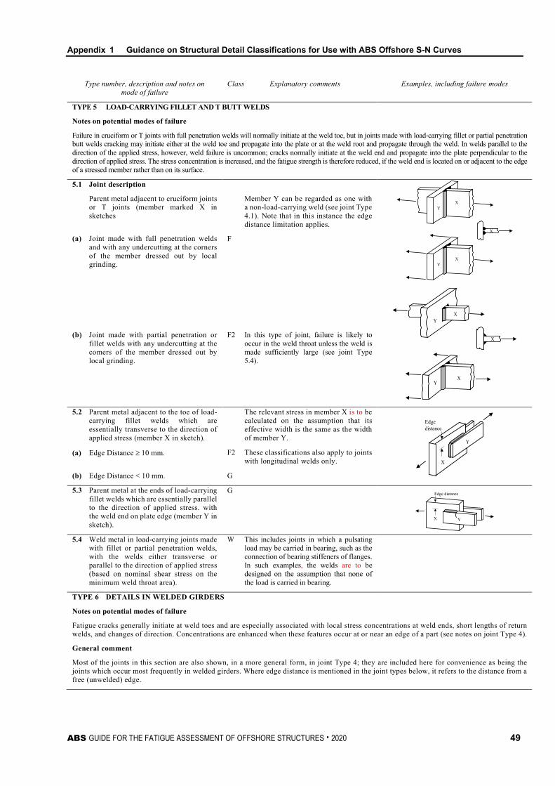
Appendix 1 Guidance on Structural Detail Classifications for Use with ABS Offshore S-N Curves
ABS GUIDE FOR THE FATIGUE ASSESSMENT OF OFFSHORE STRUCTURES . 2020 49
Type number, description and notes on mode of failure
Class Explanatory comments Examples, including failure modes
TYPE 5 LOAD-CARRYING FILLET AND T BUTT WELDS
Notes on potential modes of failure
Failure in cruciform or T joints with full penetration welds will normally initiate at the weld toe, but in joints made with load-carrying fillet or partial penetration butt welds cracking may initiate either at the weld toe and propagate into the plate or at the weld root and propagate through the weld. In welds parallel to the direction of the applied stress, however, weld failure is uncommon; cracks normally initiate at the weld end and propagate into the plate perpendicular to the direction of applied stress. The stress concentration is increased, and the fatigue strength is therefore reduced, if the weld end is located on or adjacent to the edge of a stressed member rather than on its surface.
5.1 Joint description
XY
XY
X
Parent metal adjacent to cruciform joints or T joints (member marked X in sketches
Member Y can be regarded as one with a non-load-carrying weld (see joint Type 4.1). Note that in this instance the edge distance limitation applies.
(a) Joint made with full penetration welds and with any undercutting at the corners of the member dressed out by local grinding.
F
XY
X
XY
(b) Joint made with partial penetration or fillet welds with any undercutting at the comers of the member dressed out by local grinding.
F2 In this type of joint, failure is likely to occur in the weld throat unless the weld is made sufficiently large (see joint Type 5.4).
5.2 Parent metal adjacent to the toe of load-carrying fillet welds which are essentially transverse to the direction of applied stress (member X in sketch).
The relevant stress in member X is to be calculated on the assumption that its effective width is the same as the width of member Y.
X
Y
Edgedistance
(a) Edge Distance ≥ 10 mm. F2 These classifications also apply to joints with longitudinal welds only.
(b) Edge Distance < 10 mm. G
5.3 Parent metal at the ends of load-carrying fillet welds which are essentially parallel to the direction of applied stress. with the weld end on plate edge (member Y in sketch).
G
X Y
Edge distance
5.4 Weld metal in load-carrying joints made
with fillet or partial penetration welds, with the welds either transverse or parallel to the direction of applied stress (based on nominal shear stress on the minimum weld throat area).
W This includes joints in which a pulsating load may be carried in bearing, such as the connection of bearing stiffeners of flanges. In such examples, the welds are to be designed on the assumption that none of the load is carried in bearing.
TYPE 6 DETAILS IN WELDED GIRDERS
Notes on potential modes of failure
Fatigue cracks generally initiate at weld toes and are especially associated with local stress concentrations at weld ends, short lengths of return welds, and changes of direction. Concentrations are enhanced when these features occur at or near an edge of a part (see notes on joint Type 4).
General comment
Most of the joints in this section are also shown, in a more general form, in joint Type 4; they are included here for convenience as being the joints which occur most frequently in welded girders. Where edge distance is mentioned in the joint types below, it refers to the distance from a free (unwelded) edge.

Appendix 1 Guidance on Structural Detail Classifications for Use with ABS Offshore S-N Curves
50 ABS GUIDE FOR THE FATIGUE ASSESSMENT OF OFFSHORE STRUCTURES . 2020
Type number, description and notes on mode of failure
Class Explanatory comments Examples, including failure modes
6.1 Parent metal at the toe of a weld connecting a stiffener, diaphragm, etc. to a girder flange.
Edge distance refers to distance from a free (i.e., unwelded) edge. In this example, therefore, it is not relevant as far as the (welded) edge of the
Edgedistance
(a) Edge distance ≥ 10mm (see joint Type 4.2).
F Web plate is concerned. For reason for edge distance see note on joint
(b) Edge Distance < 10 mm. G Type 2.
6.2 Parent metal at the end of a weld connecting a stiffener, diaphragm, etc. to a girder web in a region of combined bending and shear.
E This classification includes all attachments to girder webs.
6.3 Parent metal adjacent to welded shear connectors.
Edge distance
(a) Edge distance ≥ 10mm. F
(b) Edge distance < 10mm (see Type 4.2). G
6.4 Parent metal at the end of a partial length welded cover plate, regardless of whether the plate has square or tapered ends and whether or not there are welds across the ends.
G This Class includes cover plates which are wider than the flange. However, such a detail is not recommended because it will almost inevitably result in undercutting of the flange edge where the transverse weld crosses it, as well as involving a longitudinal weld terminating on the flange edge and causing a high stress concentration.
6.5 Parent metal adjacent to the ends of discontinuous welds (e.g., intermittent web/flange welds, tack welds unless subsequently buried in continuous runs).
E This also includes tack welds which are not subsequently buried in a continuous weld. This may be particularly relevant in tack welded backing strips. Note that the existence of the cope hole is allowed for in the joint classification
Ditto. Adjacent to cope holes. F It is not to be regarded as an additional
stress concentration.
TYPE 7 DETAILS RELATING TO TUBULAR MEMBERS
7.1 Parent material adjacent to the toes of full penetration welded nodal joints.
T In this situation, design is to be based on the hot spot stress as defined in Section 3 of this Guide.
7.2 Parent metal at the toes of welds associated with small (≤ 150 mm in the direction parallel to the applied stress) attachments to the tubular member.
F
Ditto, but with attachment length > 150 mm.
F2

Appendix 1 Guidance on Structural Detail Classifications for Use with ABS Offshore S-N Curves
ABS GUIDE FOR THE FATIGUE ASSESSMENT OF OFFSHORE STRUCTURES . 2020 51
Type number, description and notes on mode of failure
Class Explanatory comments Examples, including failure modes
7.3 Gusseted connections made with full penetration or fillet welds. (But note that full penetration welds are normally required).
F Note that the design stress must include any local bending stress adjacent to the weld end.
W For failure in the weld throat of fillet welded joints.
7.4 Parent material at the toe of a weld attaching a diaphragm or stiffener to a tubular member.
F Stress is to include the stress concentration factor due to overall shape of adjoining structure.
7.5 Parent material adjacent to the toes of circumferential butt welds between tubes.
In this type of joint, the stress is to include the stress concentration factor to allow for any thickness change and for fabrication tolerances.
(a) Weld made from both sides with the weld overfill dressed flush with the surface and with the weld proved free from significant defects by non-destructive examination.
C The significance of defects is to be determined with the aid of specialist advice and/or by the use of fracture mechanics analysis. The NDT technique is to be selected to provide the detection of such significant defects.
(b) Weld made from both sides. E
(c) Weld made from one side on a permanent backing strip.
F
(d) Weld made from one side without a backing strip provided that full penetration is achieved.
F2 Note that step changes in thickness are in general, not permitted under fatigue conditions, but that where the thickness of the thicker member is not greater than 1.15 × the thickness of the thinner member, the change can be accommodated in the weld profile without any machining.
7.6 Parent material at the toes of circumferential butt welds between tubular and conical sections.
C Class and stress are to be those E corresponding to the joint type as F indicated in 7.5, but the stress must also F2 include the stress concentration factor due
to overall form of the joint.
7.7 Parent material (of the stressed member) adjacent to the toes of bevel butt or fillet welded attachments in a region of stress concentration
F Class depends on attachment length or (see Type 4.1) but stress is to include F2 the stress concentration factor due to the
overall shape of adjoining structure.

Appendix 1 Guidance on Structural Detail Classifications for Use with ABS Offshore S-N Curves
52 ABS GUIDE FOR THE FATIGUE ASSESSMENT OF OFFSHORE STRUCTURES . 2020
Type number, description and notes on mode of failure
Class Explanatory comments Examples, including failure modes
7.8 Parent metal adjacent to, or weld metal in, welds around a penetration through the wall of a member (on a plane essentially perpendicular to the direction of stress). Note that full penetration welds are normally required in this situation.
D In this situation, the relevant stress is to include the stress concentration factor due to the overall geometry of the detail.
stress
7.9 Weld metal in partial penetration or fillet welded joints around a penetration through the wall of a member (on a plane essentially parallel to the direction of stress).
W The stress in the weld is to include an appropriate stress concentration factor to allow for the overall joint geometry.
x
x
stress
section x x

ABS GUIDE FOR THE FATIGUE ASSESSMENT OF OFFSHORE STRUCTURES . 2020 53
Appendix 2: References on Parametric Equations for the SCFs of Tubular Intersection Joints
A P P E N D I X 2 References on Parametric Equations for the SCFs of Tubular Intersection Joints*
* Note: The contents of Appendix 2 have been adapted from publications of the U.K. Health and Safety Executive. Permission from the Health and Safety Executive to use the source material is gratefully acknowledged.
Several parametric formulae have been produced for the prediction of SCFs for tubular joints, based on data from both physical and FE models.
1 Simple Joints Appendix 2, Table 1 indicates acceptable formulae for the prediction of SCFs for simple joints. These have been validated against data from large scale steel models and also checked against data from acrylic models and have been shown to provide acceptable predictions.
3 Multi Planar Joints For multi planar joints, SCFs are usually determined assuming there is no interaction between joints in different planes. However, in certain load cases, significant interaction can occur between joints in different planes. These effects, which can result in significantly different SCFs, are to be assessed using appropriate methods (e.g., expressions used in Efthymiou 1988).
5 Overlapped Joints Parametric formulae for the prediction of SCFs in overlapped joints have been published (Efthymiou 1988). They have not been validated because of the limited database available.
7 Stiffened Joints Parametric SCF formulae for ring-stiffened joints have been developed from test data (Smedley and Fisher 1990), which give the brace/chord intersection SCFs in terms of the equivalent, unstiffened joint SCFS. Equations to predict the SCF at the ring inner edge have also been given (Smedley and Fisher 1990).

Appendix 2 References on Parametric Equations for the SCFs of Tubular Intersection Joints
54 ABS GUIDE FOR THE FATIGUE ASSESSMENT OF OFFSHORE STRUCTURES . 2020
TABLE 1 SCF Matrix Tables for X, K and T/Y Joints
X Joints
Loading Position Efthy S&F
Balanced Axial
Chord Saddle Y X Chord Crown X* X* Brace Saddle Y Y Brace Crown Y Y
Balanced O.P.B Chordside Y Y Braceside Y Y
Balanced I.P.B Chordside Y Y Braceside Y Y
K Joints
Loading Position Efthy S&F
Balanced Axial Chordside X Y Braceside X Y
Unbalanced O.P.B Chordside Y Y Braceside Y Y
Balanced I.P.B Chordside Y Y Braceside YC Y
T/Y Joints
Loading Position Efthy S&F
Axial
Chord Saddle Y Y Chord Crown Y Y Brace Saddle Y Y Brace Crown YC Y
O.P.B Chordside Y Y Braceside Y Y
I.P.B Chordside Y Y Braceside Y X
Key to A2/Table 1
Y Recommend the equation YC Recommend the equation – but note that the equation is generally conservative X Not recommend the equation, since it fails to meet the acceptance criteria X* The equation cannot be recommended since there are less than 15 steel and acrylic joints in the SCF database. Efthy Efthymiou Equations (Efthymiou 1988) S&F Smedley and Fisher Equations (Smedley and Fisher 1991) NB For X Joints For the chord crown under axial load, the database is too small to recommend any equation. It is recommended
that the chord saddle SCF be applied at all periphery locations unless another appropriate method is established.

Appendix 2 References on Parametric Equations for the SCFs of Tubular Intersection Joints
ABS GUIDE FOR THE FATIGUE ASSESSMENT OF OFFSHORE STRUCTURES . 2020 55
9 References P. Smedley and P. Fisher (1990), ‘A Review of Stress Concentration Factors for Complex Tubular Joints’, Integrity of Offshore Structures Conference, Glasgow
P. Smedley and P. Fisher (1991), ‘Stress Concentration Factors for Simple Tubular Joints’, ISOPE
M. Efthymiou (1988), ‘Development of SCF Formulae and Generalized Influence Functions for Use in Fatigue Analyses’, Proceedings of Offshore Tubular Joints Conference, Surrey [with corrections]