Fatigue Analysis of Wind Turbines * -9, “f~ a, ,. *,. · led the wind turbine community to...

On the

Fatigue Analysis of Wind Turbines * “f~ -9, a,

,. *,.

,^ __. c

Issued by Sandia National Laboratories, operated for the United States Department of Energy by Sandia Corporation.

NOTICE: This report was prepared as an account of work sponsored by an agency of the United States Government. Neither the United States Government, nor any agency thereof, nor any of their employees, nor any of their contractors, subcontractors, or their employees, make any warranty, express or implied, or assume any legal liability or responsibility for the accuracy, completeness, or usefulness of any information, apparatus, product, or process disclosed, or represent that its use would not infringe privately owned rights. Reference herein to any specific commercial product, process, or service by trade name, trademark, manufacturer, or otherwise, does not necessarily constitute or imply its endorsement, recommendation, or favoring by the United States Government, any agency thereof, or any of their contractors or subcontractors. The views and opinions expressed herein do not necessarily state or reflect those of the United States Government, any agency thereof, or any of their contractors.

Printed in the United States of America. This report has been reproduced directly from the best available copy.

Available to DOE and DOE contractors from Office of Scientific and Technical Information P.O. Box 62 Oak Ridge, TN 37831

Prices available from (703) 605.6000 Web site: http://www.ntis.govlordering.htm

Available to the public from National Technical Information Service U.S. Department of Commerce 5285 Port Royal Rd Spring&Id, VA 22161

NTIS price codes Printed copy: A07 Microfiche copy: A01

SAND99-0089Unlimited ReleasePrinted June 1999

On the Fatigue Analysis of Wind Turbinesby

Herbert J. SutherlandSandia National Laboratories

P.O. Box 5800Albuquerque, New Mexico 87185-0708

Abstract

Modern wind turbines are fatigue critical machines that are typically used to produce electricalpower from the wind. Operational experiences with these large rotating machines indicated thattheir components (primarily blades and blade joints) were failing at unexpectedly high rates, whichled the wind turbine community to develop fatigue analysis capabilities for wind turbines. Ourability to analyze the fatigue behavior of wind turbine components has matured to the point thatthe prediction of service lifetime is becoming an essential part of the design process. In thisreview paper, I summarize the technology and describe the “best practices” for the fatigueanalysis of a wind turbine component. The paper focuses on U.S. technology, but cites Europeanreferences that provide important insights into the fatigue analysis of wind turbines.

iv

Acknowledgments

In this article, I have drawn upon the work of many researchers. I wish to express myappreciation to them and to the many others who have made significant contributions to theunderstanding of fatigue in wind turbines. Due to space limitations, I have not listed all of thereferences pertaining to my subject. Rather, I have tried to hit the high points and provide readerswith sufficient information to expand their reading list, as they deem necessary.

The author also wishes to offer particular thanks to a group of his technical associates who havereviewed this article, in whole or in part. Their constructive criticism has greatly enhanced thisreview article. Thanks to Henry Dodd, Craig Hansen, Don Lobitz, John Mandell, KurtMetzinger, Walt Musial and Paul Veers.

v

Table of Contents

page

1. Introduction............................................................................................................................1

2. General Fatigue Nomenclature................................................................................................3

3. Damage Rule Formulation ......................................................................................................5

3.1. Miner’s Rule .................................................................................................................53.2. Linear Crack Propagation Models .................................................................................73.3. Summary.......................................................................................................................8

4. Load Spectra ..........................................................................................................................9

4.1. Analysis of Time Series Data ....................................................................................... 104.1.1. Rainflow Counting Algorithm................................................................................. 10

4.1.1.1. Peak-Valley Sequence..................................................................................... 114.1.1.2. Digital Sampling ............................................................................................. 114.1.1.3. Range Filter .................................................................................................... 114.1.1.4. Residual Cycles............................................................................................... 124.1.1.5. Cycle Count Matrix ........................................................................................ 12

4.1.2. Typical Rainflow Counting Example....................................................................... 134.2. Analysis of Spectral Data............................................................................................. 14

4.2.1. FFT Analysis .......................................................................................................... 144.2.1.1. Random Phase ................................................................................................ 154.2.1.2. Amplitude Variations...................................................................................... 15

4.2.2. Typical Frequency Spectra Examples...................................................................... 164.3. Analytical Descriptions of Normal-Operation Load Spectra ......................................... 18

4.3.1. Narrow-Band Gaussian Formulation....................................................................... 194.3.2. Exponential Formulation ........................................................................................ 204.3.3. Generalized Curve Fitting Techniques .................................................................... 20

4.3.3.1. Weibull Distribution........................................................................................ 204.3.3.2. Higher Order Fits............................................................................................ 21

4.3.4. Low-Amplitude Truncation .................................................................................... 224.3.5. Load Parameters .................................................................................................... 234.3.6. Cycle Rate.............................................................................................................. 23

4.4. Representative Samples ............................................................................................... 244.4.1. Minimum Data Requirements ................................................................................. 244.4.2. Inflow Parameters .................................................................................................. 264.4.3. Scaling and Extrapolating Representative Samples.................................................. 28

4.5. General Topics ............................................................................................................ 294.5.1. Load Spectra Derived from Inflow Parameters ....................................................... 294.5.2. Structural Analyses ................................................................................................ 29

vi

4.5.3. Bin Size ................................................................................................................. 304.5.4. Mean Value Bins.................................................................................................... 304.5.5. Counting Cycles ..................................................................................................... 314.5.6. Equivalent Fatigue Load......................................................................................... 32

4.6. Total Load Spectrum................................................................................................... 334.6.1. Transient Events..................................................................................................... 334.6.2. Transition Cycles.................................................................................................... 334.6.3. Comment ............................................................................................................... 344.6.4. Summation of Load States ..................................................................................... 344.6.5. Partial Safety Factors ............................................................................................. 34

4.7. Off-Axis Analysis ........................................................................................................ 344.7.1. Geometric Load Parameters ................................................................................... 354.7.2. Typical Variations in Off-Axis Load Spectra........................................................... 36

4.8. Specialized Load Spectra for Testing........................................................................... 374.8.1. Variable Amplitude Test Spectrum......................................................................... 37

4.8.1.1. WISPER......................................................................................................... 374.8.1.2. U.S. Wind Farm Spectrum.............................................................................. 38

4.8.2. Load Spectra for Gears .......................................................................................... 39

5. Material Properties ............................................................................................................... 41

5.1. Characterization of Fatigue Properties ......................................................................... 425.1.1. Goodman Diagram................................................................................................. 425.1.2. General Characterizations of Fatigue Behavior ....................................................... 43

5.1.2.1. Curve Fitting S-N Data................................................................................... 435.1.2.2. Goodman Fit for Mean Stress ......................................................................... 455.1.2.3. Crack Propagation Model ............................................................................... 45

5.2. Wood.......................................................................................................................... 465.2.1. General Properties.................................................................................................. 46

5.2.1.1. Mechanical Properties..................................................................................... 465.2.1.2. Grading .......................................................................................................... 47

5.2.2. Laminated Wood.................................................................................................... 475.2.2.1. Moisture Content............................................................................................ 485.2.2.2. Attachments ................................................................................................... 48

5.2.3. Laminated Douglas Fir ........................................................................................... 485.2.3.1. Moisture Content............................................................................................ 485.2.3.2. Fatigue Properties........................................................................................... 495.2.3.3. Goodman Diagram ......................................................................................... 51

5.2.4. Other Wood Laminates .......................................................................................... 515.3. Metals ......................................................................................................................... 51

5.3.1. Steel....................................................................................................................... 525.3.2. Aluminum .............................................................................................................. 52

5.3.2.1. S-N Data Base................................................................................................ 525.3.2.2. Spectral Loading............................................................................................. 535.3.2.3. Linear Crack Propagation Data Base .............................................................. 54

vii

5.3.3. Gears ..................................................................................................................... 555.4. Fiberglass Composites ................................................................................................. 55

5.4.1. Databases............................................................................................................... 565.4.1.1. DOE/MSU ..................................................................................................... 565.4.1.2. European Database......................................................................................... 56

5.4.2. Trend Analysis ....................................................................................................... 565.4.3. General Data Trends .............................................................................................. 57

5.4.3.1. Fabric Architecture ......................................................................................... 585.4.3.2. Fiber Content.................................................................................................. 605.4.3.3. Normalization................................................................................................. 615.4.3.4. Matrix Material............................................................................................... 61

5.4.4. Modulus Changes................................................................................................... 615.4.5. Predicting Service Lifetimes ................................................................................... 63

5.4.5.1. Industrial Materials ......................................................................................... 635.4.5.2. Database Comparison ..................................................................................... 63

5.4.6. Spectral Loading .................................................................................................... 645.4.6.1. WISPER vs. WISPERX ................................................................................. 655.4.6.2. Predicted Service Lifetime .............................................................................. 65

5.4.7. Structural Details ................................................................................................... 665.4.7.1. Ply Drops ....................................................................................................... 665.4.7.2. Locally Higher Fiber Content.......................................................................... 685.4.7.3. Transverse Cracks .......................................................................................... 685.4.7.4. Environmental Effects..................................................................................... 685.4.7.5. Equilibrium Moisture Content......................................................................... 695.4.7.6. Matrix Degradation ........................................................................................ 695.4.7.7. Property Degradation ..................................................................................... 705.4.7.8. EN-WISPER Spectrum .................................................................................. 705.4.7.9. Effects of the Environment ............................................................................. 71

5.4.8. Comments.............................................................................................................. 715.5. Fatigue Limit Design ................................................................................................... 725.6. Partial Safety Factors................................................................................................... 72

6. Inflow................................................................................................................................... 75

6.1. Annual Average Wind Speed ....................................................................................... 756.1.1. Formulation............................................................................................................ 756.1.2. Typical Distributions .............................................................................................. 75

6.2. Inflow Characteristics.................................................................................................. 766.2.1.1. Turbulence ..................................................................................................... 766.2.1.2. Vertical Shear................................................................................................. 776.2.1.3. Additional Inflow Parameters.......................................................................... 776.2.1.4. Reynolds Stresses ........................................................................................... 786.2.1.5. Summary ........................................................................................................ 79

7. Solution Techniques ............................................................................................................. 81

viii

7.1. Closed Form Solution.................................................................................................. 817.1.1. Basic Assumptions ................................................................................................. 81

7.1.1.1. Annual Wind Speed Distribution..................................................................... 817.1.1.2. Cyclic Stress ................................................................................................... 817.1.1.3. Material Behavior ........................................................................................... 827.1.1.4. Damage Rule .................................................................................................. 827.1.1.5. Run Time........................................................................................................ 82

7.1.2. Solution ................................................................................................................. 827.2. Numerical Solutions .................................................................................................... 83

7.2.1. The LIFE Duo of Fatigue Analysis Codes............................................................... 837.2.1.1. Numerical Formulation ................................................................................... 837.2.1.2. Input Variables ............................................................................................... 84

7.2.2. The ASYM Code ................................................................................................... 857.2.3. Gear Codes ............................................................................................................ 86

8. Special Topics ...................................................................................................................... 87

8.1. Reliability Analysis ...................................................................................................... 878.1.1. The Farow Code .................................................................................................... 878.1.2. Economic Implications ........................................................................................... 87

8.2. Analysis of Bonded Joints............................................................................................ 888.2.1. The Bonded Joint ................................................................................................... 888.2.2. Tubular Lap Joints ................................................................................................. 89

8.2.2.1. Axial Loads .................................................................................................... 908.2.2.2. Bending Loads................................................................................................ 928.2.2.3. Geometric Considerations............................................................................... 948.2.2.4. Contraction of the Adhesive During Cure ....................................................... 96

8.2.3. Bolted Studs .......................................................................................................... 968.2.4. Adhesives............................................................................................................... 988.2.5. Comments.............................................................................................................. 98

8.3. Nondestructive Testing................................................................................................ 998.4. Full Scale Testing ...................................................................................................... 100

9. Concluding Remarks........................................................................................................... 101

10. References ..................................................................................................................... 103

11. Appendices .................................................................................................................... 121

Appendix A The Weibull Distribution ................................................................................ 121A.1. Generalized Distribution ......................................................................................... 121A.2. Special Distributions............................................................................................... 122

A.2.1. Rayleigh.......................................................................................................... 122A.2.2. Exponential..................................................................................................... 123

A.3. Time Series Relationships ....................................................................................... 123Appendix B Turbine Data .................................................................................................. 125

ix

B.1. Sandia/DOE 34-m VAWT Test Bed ....................................................................... 125B.2. Northern Power Systems 100kW Turbine ............................................................... 125B.3. Micon..................................................................................................................... 126

x

List of Tables

page

Table I. Specialized Values for the Forman Crack Growth Model........................................... 46

Table II. Typical Mechanical Property Ratios for Laminated Douglas Fir................................. 49

Table III. Predicted and Measured Percent Decrease in Longitudinal Modulus due toCracking of the ±45 Plies. ......................................................................................... 62

Table IV. Knock-Down Factors for Selected Structural Details in Tension andCompression for Approximately 70% 0° Materials. ................................................... 67

Table V. Idealized Annual Climatological Cycle for the Dutch Environment. ........................... 71

Table VI. Accelerated Climatological Cycle for the Dutch Environment. ................................... 71

xi

List of Figures

page

Figure 1. The Stress-Strain Hysteresis Loop for a Fatigue Cycle ...............................................3Figure 2. The Fatigue Cycle ......................................................................................................3Figure 3. The Fatigue Cycle at Various R-Values......................................................................4Figure 4. Extrapolated Peak in a Typical Time Series .............................................................. 11Figure 5. Typical Cycle Count Matrix for the Edgewise Bending Stress for the NPS

100 kW Turbine....................................................................................................... 13a. Range and Mean Spectra for the Cycle Count Matrix ......................................... 13b. Range Spectra for the Cycle Count Matrix ......................................................... 13

Figure 6. Typical Cycle Count Matrix for the Flapwise Bending Stress for the NPS100 kW Turbine....................................................................................................... 13a. Range and Mean Spectra for the Cycle Count Matrix ......................................... 13b. Range Spectra for the Cycle Count Matrix ......................................................... 13

Figure 7. Amplitude Spectrum for the Root Flap Bending Stress for the NPS Turbine............. 16a. Flapwise Bending Stress..................................................................................... 16b. Edgewise Bending Stress ................................................................................... 16

Figure 8. Semi-Log Plot of the Cycle Count Distribution Obtained Using an FFTAnalysis of the NPS Turbine .................................................................................... 16a. Flapwise Bending Stress..................................................................................... 16b. Edgewise Bending Stress ................................................................................... 16

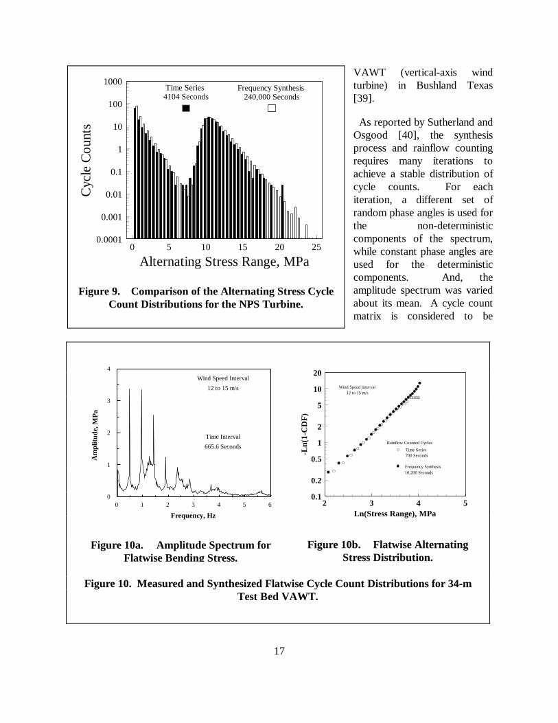
Figure 9. Comparison of the Alternating Stress Cycle Count Distributions for theNPS Turbine............................................................................................................ 17

Figure 10. Measured and Synthesized Flatwise Cycle Count Distributions for 34-mTest Bed VAWT...................................................................................................... 17a. Amplitude Spectrum for Flatwise Bending Stress ............................................... 17b. Flatwise Alternating Stress Distribution.............................................................. 17

Figure 11. Comparison of the Rainflow Counted Cycle Count Distribution and theNarrow-Band Gaussian Model for the Sandia 34-m Test Bed................................... 19a. Semi-Log Plot of the Cycle Count Distributions ................................................. 19b. Weibull Plot of the Cycle Count Distributions..................................................... 19

Figure 12. Semi-Log Plot of the Cycle Count Distribution on the NPS Turbine......................... 22a. Flapwise Bending Stress..................................................................................... 22b. Edgewise Bending Stress ................................................................................... 22

Figure 13. Comparison of the Rainflow Counted Cycle Count Distribution and theGeneralized Gaussian Model for the Sandia 34-m Test Bed...................................... 22a. Semi-Log Plot of the Cycle Count Distributions ................................................. 22b. Weibull Plot of the Cycle Count Distributions..................................................... 22

Figure 14. Comparison of the Measured and Predicted RMS Flatwise Stresses for theTest Bed for Variable Speed Operation .................................................................... 23

Figure 15. Normalized Damage Trajectory for a Micon 65/13 Turbine...................................... 25

xii

Figure 16. Damage Density Functions for the NPS 100kW Turbine .......................................... 26a. Flapwise Fatigue Load Spectrum........................................................................ 26b. Damage Density Function for Welded (m ≅ 3) Materials..................................... 26c. Damage Density Function for Composite (m ≅ 10) Blade Materials .................... 26

Figure 17. Effect of Segmented Data on the Prediction of Service Lifetimes.............................. 31Figure 18. Geometric Parameters for an Elliptical Root Section ................................................ 35Figure 19. Cycle Count Matrices for a Range of Bending Stress Directions............................... 36

a. Bending Stress at 0° ........................................................................................... 36b. Bending Stress at 45° ......................................................................................... 36c. Bending Stress at 90° ......................................................................................... 36d. Bending Stress at -30°........................................................................................ 36e. Bending Stress at -45°........................................................................................ 36f. Bending Stress at -60°........................................................................................ 36

Figure 20. Cumulative 2-Month Reference Alternating Load Spectrum..................................... 39Figure 21. High and Low Turbulence Torque Spectrum for the Micon 65................................. 39Figure 22. Time-at-Torque Histogram for the Micon 65 ........................................................... 40

a. Linear Histogram ............................................................................................... 40b. Weibull Plot ....................................................................................................... 40

Figure 23. Schematic S-N Diagram for Various Fatigue Critical Structures ............................... 41Figure 24. Typical Symmetric Goodman Diagram..................................................................... 42Figure 25. S-N Diagram for Douglas Fir/Epoxy Laminate ......................................................... 49Figure 26. Goodman Diagram at 107 Cycles for Douglas Fir/Epoxy Laminate .......................... 51Figure 27. Normalized S-N Diagram for 6063-T5 Aluminum .................................................... 53Figure 28. Fracture Mechanics Characterization for Aluminum Alloys ...................................... 54Figure 29. Crack Growth in an Aluminum Blade....................................................................... 54Figure 30. S-N Diagram for Carbonized Steel Gears ................................................................. 55Figure 31. Extremes of Normalized S-N Tensile Fatigue Data for Fiberglass

Laminates, R=0.1..................................................................................................... 57Figure 32. Extremes of Normalized S-N Compressive Fatigue Data for Fiberglass

Laminates, R = 10.................................................................................................... 58Figure 33. Extremes of Normalized S-N Reverse Fatigue Data for Fiberglass

Laminates, R = -1 .................................................................................................... 58Figure 34. Extremes of Normalized S-N Fatigue Data for a Single Family of

Fiberglass Laminates with 72% 0° Plies and 28% ±45° Plies, R = 0.1....................... 58Figure 35. Dry Fabric Samples.................................................................................................. 59Figure 36. Fatigue Sensitivity Coefficient for Fiberglass Laminates as a Function of

Fiber Content, at R = 0.1 ......................................................................................... 60a. Fatigue Sensitivity Coefficient for Various Fiber Contents in Fiberglass ............. 60b. Fatigue Sensitivity Coefficient for Unidirectional Fiberglass Laminates ............... 60

Figure 37. Effect of Matrix Material on Tensile Fatigue in a ..................................................... 61Figure 38. Reduction of Tensile Modulus in a Fiberglass Laminate with 0° and ±45°

Plies Damaged in Tensile Fatigue ............................................................................. 62

xiii

Figure 39. Goodman Diagrams for Fiberglass Composites ........................................................ 63a. Goodman Diagram based on the MSU/DOE Database ....................................... 63b. Goodman Diagram Based on the FACT Database .............................................. 63

Figure 40. S-N Diagram for a Fiberglass Laminate with 0° and ±45° Plies, underWISPER Loading Conditions................................................................................... 65

Figure 41. Typical Ply Drop Configurations .............................................................................. 66a. External Ply Drop .............................................................................................. 66b. Internal Ply Drop................................................................................................ 66

Figure 42. S-N Diagram for a Fiberglass Laminate with 0° and ±45° Plies, under Wetand Dry Environment Conditions. ............................................................................ 70

Figure 43. Weibull Probability Density Functions for Various Shape Factors............................. 75Figure 44. Variation of Low Wind Speed Start/Stop Cycles with Cut-In Power ........................ 85Figure 45. Variation of Annual Energy Production with Cut-In Power ...................................... 86Figure 46. Variation of Service Lifetime with Cut-In Power...................................................... 86Figure 47. A Typical Lap Joint.................................................................................................. 89

a. Corner of a Lap Joint ......................................................................................... 89b. Shear Stress in a Lap Joint ................................................................................. 89

Figure 48. Geometry of the Tubular Lap Joint........................................................................... 90Figure 49. Stress Distribution in Cylindrical Lap Joint Under Tensile Loads .............................. 91

a. Von Mises Stress Distribution ............................................................................ 91b. Radial (Peel) Stress Distribution......................................................................... 91

Figure 50. S-N Fatigue Data for an Aluminum-to-Fiberglass Bonded Joint................................ 91Figure 51. Tubular Lap Joint Under Bending Loads .................................................................. 92

a. Tubular Lap Joint............................................................................................... 92b. C-Scan of the Debond Failure Regions ............................................................... 92

Figure 52. 3-D Finite Element Mesh of a Circular Bond Joint.................................................... 92Figure 53. Composite Peel Stress Distribution Along the Top of the Joint (0°

Circumferential Position).......................................................................................... 93Figure 54. Partial Finite Element Meshes with Varying Adhesive Geometries............................ 93

a. Truncated Adhesive ........................................................................................... 93b. Dab of Adhesive................................................................................................. 93c. Dollop of Adhesive ............................................................................................ 93

Figure 55. Normalized Shear Stress Distribution Along the Joint............................................... 94Figure 56. Schematic of the Joint Geometries ........................................................................... 95Figure 57. Composite Peel Stress with a Dollop of Adhesive and a Tapered Adherend

for an Axial Compressive Load ................................................................................ 95Figure 58. Composite Peel Stress due to Adhesive Contraction................................................. 96Figure 59. Typical Metal Stud Design. ...................................................................................... 97Figure 60. Fatigue Behavior of a Typical Metal Stud Bonded into a Wood Laminate ................ 97Figure 61. The Sandia 34-m Test Bed Turbine ........................................................................ 125Figure 62. The Northern Power Systems 100 kW Turbine ...................................................... 126

1

1. INTRODUCTION

Somewhat over two decades ago, utility grade wind turbines were designed using static andquasi-static analyses. At best, these rather simple analyses led to over-designed turbines, and atworst, they led to premature failures. The latter is exemplified by high failure rates observed inthe early California wind farms. We, as designers, soon realized that wind turbines were fatiguecritical machines; namely, the design of many of their components is dictated by fatigueconsiderations. And, not only is this machine fatigue critical, its unique load spectrum greatlyexceeds our previous experience. This realization led to a large quantity of research that has nowmatured to the extent that state-of-the-art designs can include detailed fatigue analyses of thewind turbine.

The intent of this paper is to review these developments and to describe the “best practices” forthe fatigue analysis of wind turbine components. The paper focuses on U.S. technology but citesEuropean references that provide important insights. Most major sections are introduced with a“tutorial” section that describes basic concepts and defines pertinent terms. In all cases, anextended reference list is provided. Illustrative examples are included, as warranted. The authorassumes that the reader is acquainted with the general architecture of modern wind turbines andthe general concepts of their design. These concepts have been described in many previouspublications. The reader can draw upon several references that examine the history of windturbines [1, 2] and their design [3-7].

To facilitate this discussion, the first major section of the paper uses the Palmgren-Miner lineardamage rule [8], commonly called Miner’s Rule, to formulate the fatigue analysis of windturbines. This damage rule is currently used throughout the industry, and it is a good startingpoint to begin our discussions. After a general introduction to this rule, the rule is specialized tothe analysis of wind turbines. In the form used for the analysis of wind turbine components, therule requires three main classes of input data: the load spectra, material properties, and inflowcharacterization. Each of these components is discussed in a major section of the paper. Thefinal major section of the paper pulls these components back together into the evaluation ofservice lifetime for a wind turbine component. Specific examples from various wind turbines areused throughout the paper to illustrate important points and to provide the reader with the detailsof typical fatigue calculations for wind turbines.

3

2. GENERAL FATIGUE NOMENCLATURE

As illustrated in Fig. 1, the fatigue cycle is a closed stress-strain hysteresis loop in the stress-straintime series of a solid material. For illustrative purposes, the cycle is usually depicted as asinusoid, see Fig. 2. The maximum stress, σmax, is the largest algebraic value of the stress in thestress cycle (commonly called the peak) and the minimum stress, σmin, is the least (commonlycalled the valley). Tensile stresses are taken to be positive and compressive stresses are taken tobe negative.

The mean stress, σm, is the algebraicaverage of σmax and σmin:

σ σ σm

max min = +2

. (1)

The range of the stress cycle, σr, isdefined to be:

σ σ σr max min = − , (2)

and the amplitude of the stress cycle,σa, equals half of the range and isgiven by:

σ σ σ σa

max min r =

= 2

−2

. (3)

The R ratio is the ratio of σmin toσmax, namely,

R = min

max

σσ

. (4)

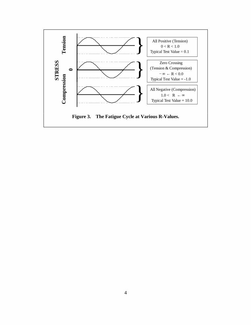
The fatigue cycle for various meanstresses and R values is depicted inFig. 3.

STR

ESS

STRAIN

1

2

0

3

4

5

6

7

8

02

3

4

5

6

7

8

1

0

1

2

3

45

6 78

STRAIN

TIME

TIME

STRESS

Figure 1. The Stress-Strain Hysteresis Loop for aFatigue Cycle.

ST

RES

S

C

ompr

essio

n

Ten

sion

0

Stress Range

Mean Stress

Minimum Stress

Stress Amplitude

Maximum Stress

Figure 2. The Fatigue Cycle.

4

STR

ESS

Com

pres

sion

Ten

sion

0

}}}

All Negative (Compression) 1.0 < R ← ∞

Typical Test Value = 10.0

Zero Crossing (Tension & Compression)

− ∞ ← R < 0.0 Typical Test Value = -1.0

All Positive (Tension)0 < R < 1.0

Typical Test Value = 0.1

Figure 3. The Fatigue Cycle at Various R-Values.

5

3. DAMAGE RULE FORMULATION

General fatigue analysis has been discussed in an exceptionally large number of textbooks,reference manuals and technical papers. The ones that I have found to be particularly useful arelisted in Refs. 9 through 14. These references provide both a general introduction and detailedanalysis techniques for the fatigue analysis of common structures. They provide a commonstarting point for fatigue analysis of wind turbines. Fatigue analyses that have been specialized tothe prediction of service lifetimes for wind turbines are discussed in Refs. 4, 6, 15 and 16.

3.1. Miner’s Rule

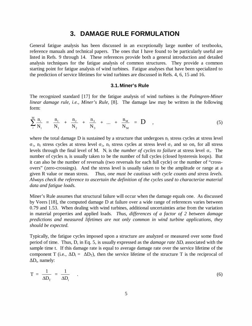
The recognized standard [17] for the fatigue analysis of wind turbines is the Palmgren-Minerlinear damage rule, i.e., Miner’s Rule, [8]. The damage law may be written in the followingform:

nN

= nN

+ nN

+ nN

+ ... + nN

= M

2

2

3

3

M

M

i

iiÂ 1

1

D , (5)

where the total damage D is sustained by a structure that undergoes n1 stress cycles at stress levelσ1, n2 stress cycles at stress level σ2, n3 stress cycles at stress level σ3 and so on, for all stresslevels through the final level of M. Ni is the number of cycles to failure at stress level σi. Thenumber of cycles ni is usually taken to be the number of full cycles (closed hysteresis loops). Butit can also be the number of reversals (two reversals for each full cycle) or the number of “cross-overs” (zero-crossings). And the stress level is usually taken to be the amplitude or range at agiven R value or mean stress. Thus, one must be cautious with cycle counts and stress levels.Always check the reference to ascertain the definition of the cycles used to characterize materialdata and fatigue loads.

Miner’s Rule assumes that structural failure will occur when the damage equals one. As discussedby Veers [18], the computed damage D at failure over a wide range of references varies between0.79 and 1.53. When dealing with wind turbines, additional uncertainties arise from the variationin material properties and applied loads. Thus, differences of a factor of 2 between damagepredictions and measured lifetimes are not only common in wind turbine applications, theyshould be expected.

Typically, the fatigue cycles imposed upon a structure are analyzed or measured over some fixedperiod of time. Thus, D, in Eq. 5, is usually expressed as the damage rate ∆Dt associated with thesample time t. If this damage rate is equal to average damage rate over the service lifetime of thecomponent T (i.e., ∆Dt = ∆DT), then the service lifetime of the structure T is the reciprocal of∆Dt, namely:

T = 1

= 1

T tD DD D . (6)

6

Again, Eq. 6 is predicated on the assumption that failure will occur when the damage equalsone, and that the damage rate computed over time t is representative of the average damage rateimposed upon the structure during its service lifetime. Namely, the number and distribution offatigue cycles contained in the sample are essentially identical to the number and distribution overthe structure’s service lifetime.

The number of cycles to failure, N in Eq. 5, is a measure of the material’s ability to endure stresscycles. This material property is typically described with an “S-N” curve. Actually, the S-Ndescription of the fatigue characteristics for a given material is a family of curves that depends onboth the mean (Eq. 1) and the range (Eq. 2) or amplitude (Eq. 3) of the stress cycle. The Rvariable (Eq. 4) is also used extensively in the description of S-N data, e.g., see Rice et al. [9].

If we assume that the fatigue cycles imposed upon the structure may be described by somefunction of σm and σa, then Eq. 5 can be written in integral form as:

D = n , N ,

d dm a

m a0-a m

σ σσ σ

σ σb gb g

∞

∞

∞zz . (7)

Alternate formulation of Eq. 7 could be written in terms of n(σm,σr) or n(σm,R). When countedover a specific period of time, the damage is typically cast as a damage rate ∆Dt, namely thedamage D accumulated in time t. Rewriting Eq. 7 to include time dependence yields:

DD Dt

t m a

m a0- a m = =

n , N ,

d dt

s ss s s sb gb g

•

•

• zz . (8)

If the damage rate computed over time t is representative of the average damage rate accumulatedby a component over its service lifetime, then the service lifetime T is the reciprocal of the damagerate computed over time t. Thus, the predicted service lifetime T, see Eq. 6, becomes:

1T

= n , N ,

d d = tt m a

m a0- a mDD s s

s s s sb gb g

•

•

• zz . (9)

For wind turbine applications, the cycle counts n(•) are typically taken to be an explicit function ofthe short-term average inflow velocity U (typically, U is based on a ten-minute average). Windspeed is chosen as an independent variable because most loads, performance parameters, andcontrol algorithms are directly related to the short-term average velocity of the inflow. Using theprobability density function pU for the inflow velocity U, Eq. 9, may be written as:

1T

= p u n , , U

N , d d du = t U0

t m a

m a0- a mDD b g b g

b g• •

•

•z zz s ss s s s , (10)

and if the turbine is only operated between a cut-in velocity of Uin and a cut-out velocity of Uout,then:

7

1T

= p u n , , U

N , d d du = t UU

U t m a

m a0- a m

in

outDD b g b gb gz zz •

•

• s ss s s s . (11)

The probability density function pU is usually taken to be the annual wind speed distribution at thesite of the wind turbine (see the discussion in section 6.2 “Inflow Characteristics” on p. 76).Equation 11 describes the damage incurred on the wind turbine during normal operation. Otherterms, typically arising from transient events, are discussed in section 4.6 “Total Load Spectrum”on p. 33. This integral equation is typically changed to a finite summation for numerical analysis[19].

3.2. Linear Crack Propagation Models

In addition to a Miner’s rule based damage analysis, linear crack propagation models [12, 13]have had successful applications to the analysis of wind turbine components. In this analysistechnique, a crack subjected to N load cycles will grow from an initial length of ao to a final lengthof af based on its crack growth rate of da/dn; namely,

a - a = dadn dnf o

0

N

e jz . (12)

The growth rate is material dependent. Typical formulations characterize this behavior in terms ofthe stress intensity factor K, which has the form:

K = y( ) a ∑ s p , (13)

where y(•) is the shape factor that is a function of specimen geometry and crack length [14]. Forvery large bodies subjected to tensile stress, y(•) is a constant equal to 1.

In an equivalent relationship to that shown in Eq. 11, Eq. 12 may be expanded to the following:

Da p d , , y

dn n , , U d d dU = U

U

Um a

0-t m a a m

in

outz zz ∑•

•

• a K K b g b gs s s s , (14)

where Km and Ka are stress intensity factors associated with the mean and alternating stress,respectively. This form is easily changed to a finite summation for numerical analysis, see Eq. 62and Sutherland and Schluter [20].

8

3.3. Summary

Thus, three sets of information are required to estimate the service lifetime of a wind turbine: thefatigue load cycles on the turbine as a function of the inflow conditions, the S-N behavior or thelinear crack growth of the material(s) being analyzed, and the annual wind speed distribution. Thefollowing three sections describe these inputs in detail and present typical examples. Whererequired, the examples have been obtained using the LIFE2 fatigue analysis code for windturbines [21]. This numerical simulation technique is described in section 7.2.1 “The LIFE Duoof Fatigue Analysis Codes” on p. 83.

9

4. LOAD SPECTRA

As implied by the formulation presented in Eq. 11, the spectrum of fatigue loads on a windturbine, i.e., n(σm,σa,U), has a significant dependence on the operational state of the turbine. InEq. 11, this dependency is described as a function of the inflow conditions. This characterizationis rather simplistic in that the operation of the turbine is dependent on many variables, only one ofwhich is the inflow velocity. To make the problem tractable, most analysts divide the operationalstates of the turbine into a series of (independent) operational states that describe the various setsof fatigue loads on the turbine. A typical division would be:

1) A series of operation states that describes the loads on the turbine during normaloperation. In a typical formulation, these states are taken to be a function of theinflow velocity. The range of the inflow velocity is from the cut-in velocity Uci of theturbine to its cut-out velocity Uco.

2) A series of “start/stop” operation states that describes the loads on the turbine duringnormal stops, emergency stops, etc.

3) A series of “buffeting” operational states that describes the loads on the turbine while itis stopped, but its blades and other structural components are being buffeted by theinflow.

4) Any additional operational states that impose significant fatigue loads on the structurethat are not covered by the other three operational states.

This division of load cases falls within the standard set of load cases that has been established bythe International Electrotechnical Commission, IEC, for the design of wind turbines [17, 22].

Once the load states are defined, each must be characterized through experimental and/oranalytical investigations. However, as wind turbines are subjected to random input from theinflow, this task can be quite difficult. Typically, the analyst will obtain a representative sample ofthe loads imposed on the turbine during each state and then weight them by their expected rate ofoccurrence. In the above list, the first and third series of operational states are weighted by theprobability density function for the annual wind speed distribution pU (see Eq. 11) and the secondstate by the number of expected events in each one of its categories. Typically, survival loadsunder extreme wind conditions are not included in the fatigue analyses.

In each operational state, the object is to obtain a numerical or analytical description of then(σm,σa,U) function. This function may take the form of tabular data or it may be an analyticalexpression. The former is commonly called a cycle count matrix, that “bins” the fatigue cycles bytheir mean, amplitude, range R value and/or sequence [23]. The functional form of choice for thedescription of n(σm,σa,U) depends on the damage rule chosen to predict service lifetimes, e.g., thelinear damage rule cited in Eq. 11. The cycle count distribution is usually presented in one ofthree forms [24]:

1) range spectrum2) range and mean spectrum

10

3) Markov matrix

These three representations are listed in increasing order of information. The range spectrum issimply a column of cycle counts, and the counts are placed in bins based upon their range, i.e., aone-dimensional function. The range and mean spectrum is a two-dimensional (2-D) matrix of thecycle counts that are placed in a two-dimensional array of bins based upon their range and mean,i.e., a two-dimensional function. The Markov matrix retains the peak and valley from each cycleand some information about their sequence. In the Markov “from-to” matrices, the sequenceinformation is a probability function that describes which peak will follow a given valley andwhich valley will follow a given peak. For linear damage analysis, Eq. 11, the sequence of thefatigue cycles is not required. Thus, characterization (1) or (2) is the characterization of choicefor the typical fatigue analysis of a wind turbine.

In this section of the paper, I describe the three primary methods for creating the n(σm,σa,U)function: time series data, frequency domain spectral data and analytical expressions. Each ofthese methods may be obtained from experimental investigations and/or analytical simulations.After the major techniques have been discussed, I will discuss related topics that arise whenconducting the fatigue analysis of wind turbines.

4.1. Analysis of Time Series Data

In many cases, the results of an experimental or an analytical investigation of the stress and strainsproduced in the turbine structure by the loads imposed upon it are plots that follow the stress(strain) as a function of time. These time series are typically generated from an experimental oranalytical investigation of the turbine. Detailed discussions of the techniques used to obtain thesetime series are beyond the scope of this report. And, they have been discussed extensively inprevious reports, e.g., Madsen [25] and Pedersen [26]. For the purposes of this report, I assumethat the necessary time series are available for the fatigue analysis. A few precautions related totime series data are discussed in section 4.5 “General Topics” on p. 29.

4.1.1. Rainflow Counting Algorithm

Time series data, either derived from analytical simulations or from actual measurements, havebeen studied extensively by other researchers. The wind industry has drawn upon their techniquesfor converting time series into cycle count matrices. A number of numerical techniques areavailable from these previous studies. The technique typically used in the wind turbine industry isthe rainflow counting algorithm presented in Downing and Socie [27]. A complete description ofthis algorithm is also provided in Rice et al. [9]. One adaptation of the technique to wind turbinesis described in Sutherland and Schluter [28]. Wu and Kammula [29] have developed a real-timealgorithm using rainflow-counting techniques that reduces memory requirements and speedscomputations.

The implementation presented by Downing and Socie [27], requires both a pre and a postprocessor for its implementation into a form that is useful for analysis. This section discusses this

11

counting process from the input of a time series to the final output. Also, several questions thatarise when this technique is used for the analysis of wind turbines are addressed.

4.1.1.1. Peak-Valley Sequence

The input to the rainflow counting algorithm is a simple series of peaks and valleys (troughs), i.e.,local maxima and minima, that form hysteresis loops, see Fig. 1. To convert a time series to theappropriate list, a pre-processor searches for local extremes in the series and lists them insequence [28]. Typically, the algorithm uses a change in slope as an indicator that the time seriesis going though a peak or valley. Only the magnitude of the peak or valley is then entered into therainflow counting algorithm. The algorithm defines the first point in the time series to be the firstentry in the peak-valley list.

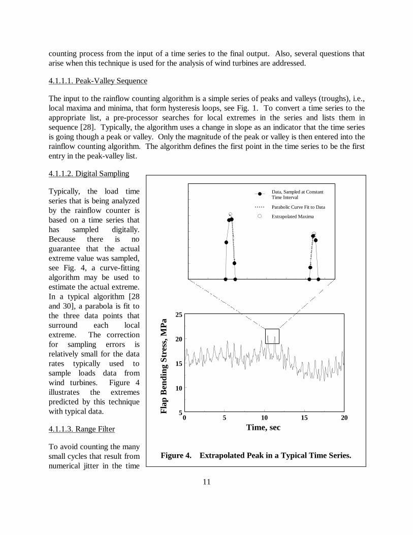
4.1.1.2. Digital Sampling

Typically, the load timeseries that is being analyzedby the rainflow counter isbased on a time series thathas sampled digitally.Because there is noguarantee that the actualextreme value was sampled,see Fig. 4, a curve-fittingalgorithm may be used toestimate the actual extreme.In a typical algorithm [28and 30], a parabola is fit tothe three data points thatsurround each localextreme. The correctionfor sampling errors isrelatively small for the datarates typically used tosample loads data fromwind turbines. Figure 4illustrates the extremespredicted by this techniquewith typical data.

4.1.1.3. Range Filter

To avoid counting the manysmall cycles that result fromnumerical jitter in the time

Data, Sampled at Constant Time Interval

Parabolic Curve Fit to Data

Extrapolated Maxima

Flap

Ben

ding

Str

ess,

MPa

0 5 10 15 205

10

15

20

25

Time, sec

Figure 4. Extrapolated Peak in a Typical Time Series.

12

series and/or to eliminate the many small cycles that do not contribute significantly to the damageof the wind turbine, a range filter is typically used. This filter requires that successive localextremes must differ by a minimum value, typically called the threshold, before they areconsidered to be extremes that should be retained by the filter. Various algorithms have beenproposed for processing time series data. A useful one is the racetrack filter described by Veerset al. [30].

4.1.1.4. Residual Cycles

The rainflow counting algorithm proceeds by matching peaks and valleys to form closedhysteresis loops. When the algorithm reaches the end of time-series data record, a series ofunmatched peaks and valleys remains unclosed and, therefore, are not counted by the algorithm.These so-called “half-cycles” typically include the largest peak and valley in the record and theymay also include other large events. Thus, the potentially most damaging events (the largestcycles) contained in the time series are not counted by the classical formulation of the rainflowalgorithm. If desired, the rainflow counting algorithm can be easily modified to include thesehalf–cycles in the cycle count [28, 29].

Various researchers have proposed several techniques for handling these half-cycles in windturbine applications. Some ignore them, some count them as half of a complete cycle (hence,their name), and others count them as full cycles. The latter is the most conservative approach.However, the recommended practice, as stated in Madsen [25], is to treat all unclosed cycles ashalf cycles. This recommendation is currently being retained in the IEC standards [31].

4.1.1.5. Cycle Count Matrix

The output of the rainflow counting algorithm is a characterization of the stress (strain) cycle byits maximum and its minimum value. The counting algorithm counts each cycle in its order ofoccurrence. The post-processor then puts this information into a form suitable for the fatigueanalysis package.

The first task of the postprocessor is to convert this characterization of a fatigue cycle to thatused by the fatigue analysis. As discussed above, the final data representation typically takes oneof three forms: range spectra, range and mean spectra, and Markov matrices. Thus, the post-processor’s first task is to convert the maximum/minimum representation of the data into one ofthese forms. The second task is to format the data for processing by the damage analysis. Thisstep typically includes placing each cycle in the appropriate cycle-count bin1 and writing thatinformation to file. The output file can take many forms, depending on the analysis and numericaltechniques being used to determine the damage. Thus, a specialized post-processor is usuallyrequired for each fatigue analysis technique.

1 A fatigue cycle is added to a cycle count bin if its magnitude falls within the bounds of the bin. All cycle countswithin a bin are assumed to have the same magnitude. This characteristic magnitude is a function of the endpoints of the bin. An example of a 2-D bining operation is shown in the next section of the paper.

13

4.1.2. Typical Rainflow Counting Example

A typical rainflow counted load spectrum is shown in Fig. 5 for the edgewise-bending stress andin Fig. 6 for the flapwise-bending stress. These data were collected from an NPS 100-kW turbinein Altamont Pass, California [32]. The data are for normal operating conditions with a meaninflow velocity of 11.0 m/s. As shown in Figs. 5a and 6a, the distribution of cycle counts that isobtained from the rainflow counting algorithm was post-processed into a 2-D matrix that placeseach cycle into a cycle count bin based upon its mean and range (or amplitude). In this form, acycle count is added to bin (i,j) when

s s sm i-1 m m i b g b g b g< £ , (15)

s s sa j-1 a a j b g b g b g< £ , (16)

Figure 6a. Range and Mean Spectra forthe Cycle Count Matrix.

0 5 10 15 20 250.01

0.03

0.1

0.3

1

3

10

30

100

Alternating Stress Range, MPa

Cyc

le C

ount

s

Figure 6b. Range Spectra for the CycleCount Matrix.

Figure 6. Typical Cycle Count Matrixfor the Flapwise Bending Stress for the

NPS 100 kW Turbine.

Figure 5a. Range and Mean Spectra forthe Cycle Count Matrix.

0 5 10 15 20 250.01

0.03

0.1

0.3

1

3

10

30

100


Cyc

le C

ount

s

Figure 5b. Range Spectra for the CycleCount Matrix.

Figure 5. Typical Cycle Count Matrixfor the Edgewise Bending Stress for the

NPS 100 kW Turbine.

14

where bin (i,j) has the a maximum mean stress of (σm)i and a maximum alternating stress (range)of (σa)j and the cycle being counted has a mean stress of (σm) and a range (or amplitude) of (σa).The width of each of the bins in this matrix can significantly influence the fatigue calculations.See the guidelines discussed in section 4.5 “General Topics” on p. 29.

The 2-D form for the cycle count matrix may be simplified to a 1-D form for analysis (as notedabove) and/or for presentation of results. Figures 5b and 6b illustrate typical 1-D distributions ofthe range of the cycle counts. The 1-D distributions in these two figures are derived from the 2-Dcycle count matrix by holding the range constant and summing over all means. In many analyses,the 1-D distribution is used, because the range of mean stresses is typically not important for windturbine predictions. This observation is discussed in section 4.5.4 “Mean Value Bins” on p. 30

4.2. Analysis of Spectral Data

Typically the development of the cycle count function n(σm,σa,U) from experimental or analyticaldata depends heavily on time series data. However, many structural analysis techniques yieldfrequency-domain stress spectra, and a large body of experimental loads (stress) data is reportedin the frequency domain. To permit the fatigue analysis of this class of data, several approacheshave been developed to obtain cycle counts from frequency spectra. In one technique, a series ofcomputational algorithms based on Fourier analysis techniques has been developed [33, 34]. Inanother technique, rainflow ranges are theoretically estimated directly from the power spectraldensity (PSD) function for the turbine [35, 36]. Only the former technique will be discussed here.

4.2.1. FFT Analysis

The Fourier analysis technique developed by Sutherland [33, 34] uses an inverse Fast FourierTransform (FFT) to transform the frequency spectrum to an equivalent time series suitable forcycle counting [37]. In this formulation, the input frequency spectrum is taken to be a uniformseries of N components with frequency intervals of ∆f. The spectrum is input as a series ofpositive amplitudes Ai and phase angles φi , i = 1, N. Most FFT algorithms are optimized forvalues of N that are a power of 2.

The inverse FFT algorithm converts the frequency spectrum into a time series of the form:

s t FFT A f fj j

N

i i i

Nd i b g b g{ }=−

==

1

21

1,φ , (17)

where the ith component of the amplitude spectrum corresponds to a frequency of

f = i -1 fi b gD , where i = 1 , ... , N, (18)

the jth component of the time series corresponds to a time of

t = j -1 tj b gD , where j = 1 , ... , 2N, (19)

15

and,

D Dt = 1

2 N f . (20)

The output time series has a total time length T equal to

T = 2 N = 1f

D Dt . (21)

Thus, the final output of the algorithm is a time-series that may be counted using the rainflowcounting algorithm cited above.

The edgewise blade spectrum for a HAWT typically shows a very strong deterministic signal thatis the direct result of the gravity loads. This observation led Sutherland [33] to develop analternate formulation of the FFT shown in Eq. 17 that permits large deterministic signals to behandled efficiently. This alternate formulation is not reproduced here.

4.2.1.1. Random Phase

The frequency spectrum of the operating loads on a wind turbine blade contains two classes ofsignals. The first is a deterministic or “steady” signal that is obtained by averaging the time seriesdata as a function of the position of the rotor (the azimuth-average). The second signal in thespectrum is the random (non-deterministic) variation about the azimuth-average. These randomcomponents in the distribution imply that the synthesis of a time series from a frequency spectrumfor wind turbines does not have a unique solution, as implied by Eqs. 17 through 21.

Akins [37, 38] handled the synthesis of both signals using the average amplitude spectrum with arandom phase angle for each component. He concludes, however, that the synthesis processwould be more realistic if the phase angles used in the synthesis process have both deterministicand random components. In particular, he notes that the phase angles for the azimuth-averagecomponents are essentially deterministic, and, therefore, the components of the spectra thatcorrespond to the azimuth-average signal should have deterministic phase angles. And he furthersuggests that the remaining components be synthesized using random phase angles.Computationally, the non-uniqueness of the input phase angles in the frequency spectrum impliesthat much iteration is required to achieve a statistically meaningful result.

4.2.1.2. Amplitude Variations

The frequency spectra for typical wind turbines vary significantly about the average spectrum dueto the random nature (both in time and in space) of the inflow. Two classes of variations arenoted: the first is the random (non-deterministic) variation of the spectral amplitudes about theiraverage at a constant average wind speed and the second is the variation of the time series withwind speed. The variation of the latter is typically handled by using multiple wind speed bins inthe fatigue analysis, see the discussion above. But, the variation of the former must be handled

16

within each wind speed bin. Sutherland [33] presents one technique for handling this variation inamplitude. His technique is used in the example presented next.

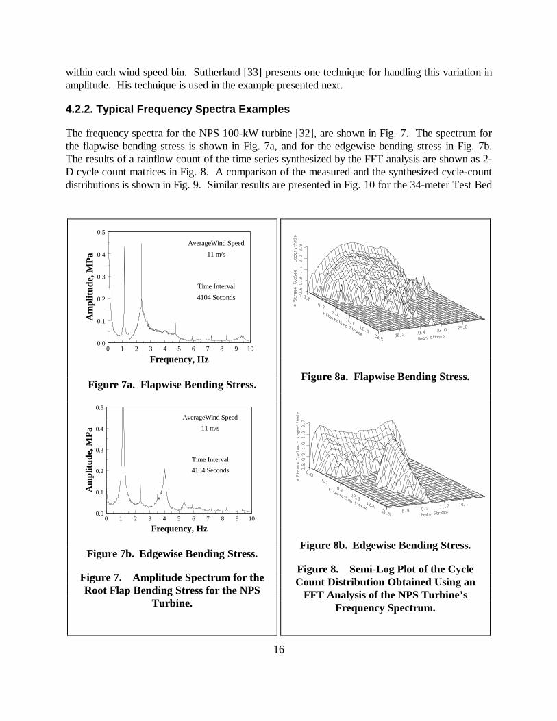
4.2.2. Typical Frequency Spectra Examples

The frequency spectra for the NPS 100-kW turbine [32], are shown in Fig. 7. The spectrum forthe flapwise bending stress is shown in Fig. 7a, and for the edgewise bending stress in Fig. 7b.The results of a rainflow count of the time series synthesized by the FFT analysis are shown as 2-D cycle count matrices in Fig. 8. A comparison of the measured and the synthesized cycle-countdistributions is shown in Fig. 9. Similar results are presented in Fig. 10 for the 34-meter Test Bed

Figure 8a. Flapwise Bending Stress.

Figure 8b. Edgewise Bending Stress.

Figure 8. Semi-Log Plot of the CycleCount Distribution Obtained Using an

FFT Analysis of the NPS Turbine’sFrequency Spectrum.

0 1 2 3 4 5 6 7 8 9 100.0

0.1

0.2

0.3

0.4

0.5

Frequency, Hz

Am

plitu

de, M

Pa

AverageWind Speed

11 m/s

Time Interval

4104 Seconds


0 1 2 3 4 5 6 7 8 9 100.0

0.1

0.2

0.3

0.4

0.5

Frequency, Hz

Am

plitu

de, M

Pa

AverageWind Speed

11 m/s

Time Interval

4104 Seconds


Figure 7. Amplitude Spectrum for theRoot Flap Bending Stress for the NPS

Turbine.

17

VAWT (vertical-axis windturbine) in Bushland Texas[39].

As reported by Sutherland andOsgood [40], the synthesisprocess and rainflow countingrequires many iterations toachieve a stable distribution ofcycle counts. For eachiteration, a different set ofrandom phase angles is used forthe non-deterministiccomponents of the spectrum,while constant phase angles areused for the deterministiccomponents. And, theamplitude spectrum was variedabout its mean. A cycle countmatrix is considered to be

Time Series 4104 Seconds

Frequency Synthesis 240,000 Seconds

0 5 10 15 20 250.0001

0.001

0.01

0.1

1

10

100

1000


Cyc

le C

ount

s

Figure 9. Comparison of the Alternating Stress CycleCount Distributions for the NPS Turbine.

Figure 10. Measured and Synthesized Flatwise Cycle Count Distributions for 34-mTest Bed VAWT.

0 1 2 3 4 5 60

1

2

3

4

Frequency, Hz

Am

plitu

de, M

Pa

Wind Speed Interval12 to 15 m/s

Time Interval665.6 Seconds

Figure 10a. Amplitude Spectrum forFlatwise Bending Stress.

2 3 4 50.1

0.2

0.5

1

2

5

10

20

Ln(Stress Range), MPa

-Ln(

1-C

DF)


Rainflow Counted Cycles

Time Series700 Seconds

Frequency Synthesis10,200 Seconds

Figure 10b. Flatwise AlternatingStress Distribution.

18

stable if the normalized distribution of the cycle counts does not change when additional timeseries are synthesized and counted. For these two examples, the cycle count matrix wasconsidered stable when the normalized number of cycle counts in each stress bin stayed within ahalf cycle count of its previous value when the synthesis time was doubled.2 Also, the high-stresstail of the cycle count distribution was used to judge the stability of the synthesis process.Namely, the distribution was considered stable if the tail of the distribution was a relativelysmooth function. For the two examples discussed here, the total synthesized time required toachieve a stable cycle count distribution was approximately 240,000 seconds in the NPS turbineand 10,200 seconds for the Test Bed turbine.

The comparisons shown in Figs. 9 and 10b illustrate that time series data for the determination ofstress cycles imposed on a wind turbine blade may be effectively synthesized from averagefrequency-spectra data. Moreover, the ability of the algorithm to generate long time seriespermits the high-stress tail of the cycle count distribution to be defined within the accuracy of theinput frequency spectrum. However, the ability to fill out the tail of the distribution should notbe confused with the actual distribution of stress cycles imposed upon the turbine. Thefrequency spectra used in the analysis are still based upon a rather limited set of data, and thosespectra may not contain sufficient information to define the correct high-stress tail of thedistribution of cycle counts.

4.3. Analytical Descriptions of Normal-Operation Load Spectra

Analytical representations have been used extensively to describe cycle count distributions. Theserepresentations not only provide the analysts with closed-form solutions for the fatigue analysisbut through the insight they provide, these formulations permit incomplete data to be interpolatedand/or extrapolated to fill voids in the data. Moreover, these representations when combined withreliability analysis permit the evaluation of the effects of randomness in the input variables on thepredicted service lifetime of a wind turbine.

Several analytical expressions have been used to describe the load spectra on a wind turbine blade.These expressions are typically derived from best-fit analyses of experimental data. Most of thesuccessful expressions fall within a generalized Weibull distribution with the narrow-bandGaussian distribution (Rayleigh distribution) being used extensively to describe the load spectraon Vertical Axis Wind Turbines (VAWTs), and the exponential distribution for the load spectraon Horizontal Axis Wind Turbines (HAWTs). [Weibull probability density functions for variousshape factors are shown below in Fig. 43.] In this section of the paper we discuss both of thesetechniques and a generalized fitting technique that distorts a parent distribution to better fit theloads on the machine.

2 The stability of a cycle count matrix (distribution) can also be defined based on the damage rate. Namely, thecycle count distribution is considered stable if the damage rate represented by these cycles changes by some smallpercentage when the synthesis time is increased significantly.

19

4.3.1. Narrow-Band Gaussian Formulation

One of the first uses of an analytical expression to describe the load spectra on a blade was thecharacterization of the load spectra on VAWTs using a narrow-band Gaussian formulation byMalcolm [41, 42], Veers [18, 43-45] and Akins [46]. In this formulation, the distribution of cyclecounts takes the form of a Rayleigh distribution, a specialized form of the general Weibulldistribution (see Appendix A). For this distribution, the Weibull shape factor, α, has a value of 2.This distribution may be written in the following form:

p exp -

2 |Ua

U2

a2

U2σ

σσ

σσ

= LNM

OQP

LNM

OQP , (22)

where the probability density function pσ|U of the cyclic stress σa is a function of the standarddeviation of the cyclic stress σU at a wind speed U. To convert this probability density functioninto cycle counts, the cycle count rate, which is discussed in section 4.3.6 “Cycle Rate” on p. 23,is required. The cycle count distribution is obtained by multiplying the probability densityfunction shown in Eq. 22 by the cycle count rate.

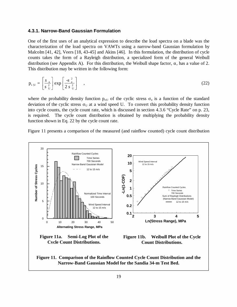
Figure 11 presents a comparison of the measured (and rainflow counted) cycle count distribution

Figure 11. Comparison of the Rainflow Counted Cycle Count Distribution and theNarrow-Band Gaussian Model for the Sandia 34-m Test Bed.

0 10 20 30 40 500

5

10

15

20


Num

ber

of S

tres

s C

ycle

s


Normalized Time Interval100 Seconds


Time Series

Narrow Band Gaussian Model

12 to 15 m/s

700 Seconds

Figure 11a. Semi-Log Plot of theCycle Count Distributions.

2 3 4 50.1

0.2

0.5

1

2

5

10

20


-Ln(

1-C

DF)




Sum of Rayleigh Distributions (Narrow Band Gaussian Model)

12 to 15 m/s

Figure 11b. Weibull Plot of the CycleCount Distributions.

20

and its Gaussian approximation for the 12 to 15 m/s wind speed bin for the 34-meter Test BedVAWT in Bushland Texas [39]. This figure illustrates the very good agreement between themeasured and modeled cycle count distributions in the body and the tail of the distribution. Asimplied in this figure, this technique is only used to describe the distribution of the fatigue cycleswith respect to their alternating stress component. In cases where the S-N material propertiesare a function of the mean stress, this formulation of the cycle count distribution implies that thedamage calculations must be based on a constant (non-zero) mean stress across the entiredistribution [43].

4.3.2. Exponential Formulation

The exponential distribution used by Jackson [47, 48], Kelley [49, 50] and Kelley and McKenna[51] is also contained in the generalized Weibull distribution, see Appendix A. For thisdistribution, the Weibull shape parameter α has a value of 1. The distribution may be written inthe following form:

p exp -

= exp -

|UU

a

U U

a

Uσ σ

σσ σ

σσ

= LNM

OQP

LNM

OQP

LNM

OQP

LNM

OQP

1 1 , (23)

where the probability density function pσ|U of the cyclic stress σa at a particular wind speed U is afunction of the standard deviation of the cyclic stress σU (in this case, σU is equivalent to the meanof the cyclic stress σU ). Again, the mean stress is assumed to be a constant across thisdistribution of cycle counts.

The distribution function that was proposed by Kelley [49] is actually the sum of threedistributions, with the exponential distribution describing the high-stress tail of the distribution. AGaussian distribution is used to describe the low-stress region and a log-normal distribution isused to describe the transition between the low and high stress regions.

4.3.3. Generalized Curve Fitting Techniques

4.3.3.1. Weibull Distribution

The Rayleigh and exponential distributions cited above can be generalized to the Weibulldistribution. In its generalized form, the distribution becomes

p exp -

|Ua

-1

aσ

α ααβ

σβ

σβ

= LNM

OQPLNM

OQP

LNM

OQP

RS|T|UV|W|

, (24)

where the Weibull parameters α and β can be expressed as functions of the mean and standarddeviation of the cycle count distribution (Appendix A).

21

4.3.3.2. Higher Order Fits

A generalized curve fitting technique, named FITTING, that provides fourth order fits to the datahas been proposed by Winterstein et al. [52, 53]. This formulation optimally retains the statisticalinformation of the high-stress level data (i.e., the tail of the cycle count distribution) by distortinga parent distribution to fit the first four statistical moments of the data. Importantly, thistechnique distorts the parent distribution when the data indicate that the distribution differs fromthe parent distribution. The tail is fit to the observed distribution by warping the parentdistribution (two parameter distributions) using two additional parameters: the skewness (3rd

moment of the distribution) and the kurtosis (4th moment of the distribution). Three parentdistributions are available in the FITTING routine: a Gaussian, a Weibull, and a Gumbel. Insubsequent analyses, Winterstein and Kashef [54] demonstrated that for the one-sideddistributions typically encountered in cycle-counts, three-moment distributions provide better fitsof the data than four-moment distributions.

As discussed above, previous fits to cyclic load distributions from wind turbines have emphasizedRayleigh and exponential distributions, which are special cases of the Weibull distribution.Weibull distributions can model a wide range of behaviors with two parameters to describe thecentral tendency of the distribution (i.e., the body of the distribution) and the spread of thedistribution (i.e., the tail of the distribution). With its versatility and the previous emphasis thathas been placed on its use, a generalized Weibull fit will be used exclusively in the examplespresented here.

Typical generalized curve fits for the data presented in Figs. 8 and 11 are given in Figs. 12 and 13,respectively. As illustrated in these figures, the fit has excellent agreement with the data in thebody and the tail of the distribution. And, as discussed above, the low-amplitude portion of thedistribution is not included in the fit because it is of no consequence in the damage calculations.Moreover, Winterstein et al. have recommended that the curve fit should not include the low-amplitude cycles because they will decrease the accuracy of the fit in the body and the tail ofdistribution where the damage is concentrated for typical blade materials. As with its specializedforms, the generalized technique only describes the distribution of the fatigue cycles with respectto their alternating stress component. And, the mean stress is assumed to be a constant acrossthis distribution of cycle counts. The elimination of the low-amplitude stress cycles and the meanstress variations from the fitting process are particularly evident when Fig. 8 is compared to Fig.12.

The importance of defining the correct functional form for the distribution of cycle counts isdiscussed in Sutherland and Butterfield [55]. When the same cycle count distribution was fit withan exponential distribution and with a Rayleigh distribution, the former was found to contain tentimes more damage than the latter. This significant increase in damage is a direct result of thecycles contained in the tail of the distributions, with the exponential predicting more cycles in thetail than the Rayleigh. Thus, the fitting technique is extremely important, and its form should notbe prejudged. And, by using the generalized fitting routine, the fitting algorithm obtains the bestfit to the data by choosing both the form of the underlying distribution and its distortion.

22

4.3.4. Low-Amplitude Truncation

The curve-fitting procedures described above are implicitly tied to the assumption that the initialportion of the cycle count distribution is not important in a damage calculation. For example, theanalytical distribution shown in Fig. 13a matches the measured cycle counts very well aboveapproximately the 14 MPa bin. Below this bin, the distribution falls to zero, while the measureddistribution increases dramatically, with the smallest bin having several thousand counts. Asdiscussed in section 4.4.1 “Minimum Data Requirements” on p. 24 and illustrated by Fig. 16,these counts are typically not significant in the determination of damage and may be ignored in


Generalized Gaussian Model

12 to 15 m/s


0 10 20 30 40 500

5

10

15

20


Num

ber

of S

tres

s C

ycle

s

Figure 13a. Semi-Log Plot of the CycleCount Distributions.


8 10 20 50 1000.2

0.5

1

2

5

10

20

Stress Range, MPa

- ln

[ 1 -

CD

F ]



Generalized Weibull Fit

Figure 13b. Weibull Plot of the CycleCount Distributions.

Figure 13. Comparison of the RainflowCounted Cycle Count Distribution andthe Generalized Gaussian Model for the

Sandia 34-m Test Bed.



Figure 12. Semi-Log Plot of the CycleCount Distribution on the NPS Turbine.

23

the curve fitting procedure. In special cases, these low-damage (approaching zero) cycles can beincluded in the damage analysis by maintaining them as true cycle count bins, as shown in Fig. 12or by adding multiple piecewise distributions together [49].

4.3.5. Load Parameters

For all of the above formulations, the functional relationship between the stress state parametersand the characteristics of the inflow must be determined before they can be applied. As cited inEqs. 22 and 23, the Rayleigh and the exponential formulations are one-parameter models thatdescribe this functionalrelationship. In both cases, thisparameter is related to the RMSblade stress σU; which is thenrelated to the average inflowwind speed U. To date, themajority of the workcharacterizing this relationshipuses the Rayleigh model tocharacterize VAWT loads. Atypical relationship between σU

and U, for the 34-m Test Bedturbine [39], is shown in Fig. 14[56]. This relationship istypically characterized as apiece-wise, linear relationshipfor analysis [57].

As the formulations areextended to higher orders, thedescriptions of the parameterset required by the models canbecome significantly morecomplicated. Higher ordercharacterizations are reported inLange and Winterstein [58], Kashef and Winterstein [59] and Veers and Winterstein [60].

4.3.6. Cycle Rate

In most of these formulations, the distribution of stress cycles is represented as a normalizeddistribution. Thus, the total number of stress cycles contained in the distribution (or, moreprecisely, the average rate at which stress cycles are imposed upon the structure) is anotherparameter required by the fitting procedure. There have been several techniques proposed forassessing the value of this variable.

0 5 10 15 20 250

5

10

15

Wind Speed, m/s

RM

S St

ress

, MPa

Variable Speed

Measured Stresses

Analytical Stresses

Figure 14. Comparison of the Measured and PredictedRMS Flatwise Stresses for the Test Bed for Variable

Speed Operation.

24

The first, and the most obvious technique, is to use one of the cycle counting techniques discussedabove to determine the average rate of cycle accumulation. This technique was used bySutherland and Veers [61] in their evaluation of the effectiveness of these models and in thedetailed analysis of the fatigue loads on the Sandia 34-m Test Bed [57]. Other methods, originallyproposed by Veers, use the dominant frequency of blade vibration [43] or the rate of mean levelcrossings [18] as the average cycle rate. In these two methods, the frequency is usually chosen tobe independent of wind speed. Typically for VAWTs, the cycle rate is chosen to be three timesthe rotational rate of the turbine for edgewise stresses and two times for flatwise stresses. ForHAWTs, the edgewise rotation cycle rate is chosen equal to the rotation rate. In theircomparisons of results, Ashwill et al. [57] illustrate that the measured cyclic rates were higherthan the estimated rate, but, when the damage from these two rates was compared, the differenceswere not significant.

4.4. Representative Samples

As indicated in Eq. 11, the normal operation cyclic loads are typically weighted using the annualwind speed distribution and then summed to find the total operating load spectrum. This analysistechnique implicitly assumes that each normal-operation wind-speed bin contains a representativesample for all of the inflow conditions characterized by the short-term average inflow velocity.Each sample is typically extremely short in time when compared to the design lifetime of theturbine, i.e., minutes or hours as opposed to years.

As discussed by Winterstein (his comments are reported in Sutherland and Butterfield [55]),representative samples are adequate for this application because the fatigue analysis needs only toaccurately estimate the mean damage rate at a given operational state. In other words, fatigueanalysis should not require more loads data if the service lifetime is increased from 30 to 60 years,say. This observation is especially important because it implies that the fatigue analysis can bebased on representative samples that can then be scaled to the lifetime of the turbine. However,the representative sample conjecture requires that the sample be truly representative and thatstatistical models can use this sample to extrapolate from relative short-term data to long-termdata.

4.4.1. Minimum Data Requirements

The importance of obtaining a truly representative sample has been graphically presented inSutherland and Veers [61]. In this paper, Sutherland and Veers demonstrate that the damagecontained in separate 10-minute data segments, taken for normal operation of the 34-m Test Bedat a constant mean wind speed, can vary by two orders of magnitude.

In a follow-on analytical study, Kelley and Sutherland [62] examined damage predictions for aMicon 65/13 turbine installed in Row 37 of a 41-row wind farm in San Gorgonio Pass, California.They examine accumulated damage in the blades during a typical diurnal variation of the inflow atthe San Gorgonio site. Of the total 144 ten-minute simulations, 37 simulations had a mean inflowvelocity between 11 and 13 m/s. The normalized damage trajectory based on the sequentialanalysis of the 37 ten-minute simulations is illustrated in Fig. 15. In this plot, the average damage

25

rate for the 37 simulations isnormalized to one. Theaverage nominal damage rateis then plotted as a functionof the number of ten-minuterecords included in theaverage. This plotdemonstrates that the damagestays within approximately +7and -25 percent of its averagevalue after the first 19 10-minute simulations (3.1hours). Thus, one wouldsurmise that a representativesample requires a minimum of19 simulations for thisoperational state and turbine.However, if sequencing in the

trajectory is changed, a very different result is obtained. Namely, consider the upper and lowerbound trajectories shown in the figure. In these plots, the simulations are added in the order ofthe damage they contain, with the upper bound sorted in descending order and the lower boundsorted in ascending order. First, these trajectories demonstrated that the simulation containing thesmallest damage underestimates the average damage by almost two orders of magnitude and thelargest overestimates the average damage by over one order of magnitude. And, the samplerequires almost all of 37 simulations before it stabilizes to the average damage rate. Thus, whenthe trajectory is based on ordered members of the data set, the trajectory essentially does notstabilize until all members of the set have been added because the sample is not representative.Techniques for insuring that a representative sample has been obtained are typically based onobtaining a representative set of inflow conditions, such as turbulence intensity in each mean windspeed bin. Criteria for this technique are discussed in section 4.4.2 “Inflow Parameters” on p. 26.

In another study, Winterstein and Lange [52] note that the data requirement for representativesamples also depends on the coefficient of variation (COV) that is acceptable in the damagecalculation. Using the data from the Northern Power Systems 100-kW turbine and assumedvalues for the COV of the damage and material variability, they estimated that at least 280minutes (4.7 hours) are required to define the cyclic load distribution for a composite blade.

As reported in Sutherland and Butterfield [55], Winterstein notes another critical concept whendetermining minimum data requirements for fatigue analyses. In particular, fatigue analysesdepend heavily on both the loads and the fatigue behavior of the material; e.g., the slope of theS-N curve (i.e., m in Eq. 34, below) used to define damage rate (Eq. 8). As shown in Fig. 16, thedamage contained in the flapwise bending stress spectrum, Fig. 16a (also shown in Fig. 6b), isconcentrated in the body of the distribution when the exponential slope m is small (typical ofwelded materials), Fig. 16b, and in the tail of the distribution when the slope is large (typical of

0 10 20 30 400.001

0.01

0.1

1

10

100

Number of 10-min Blocks

Nor

mal

ized

Dam

age

Average

Upper and Lower Limits

Sequencial Count

Figure 15. Normalized Damage Trajectory for a Micon65/13 Turbine.

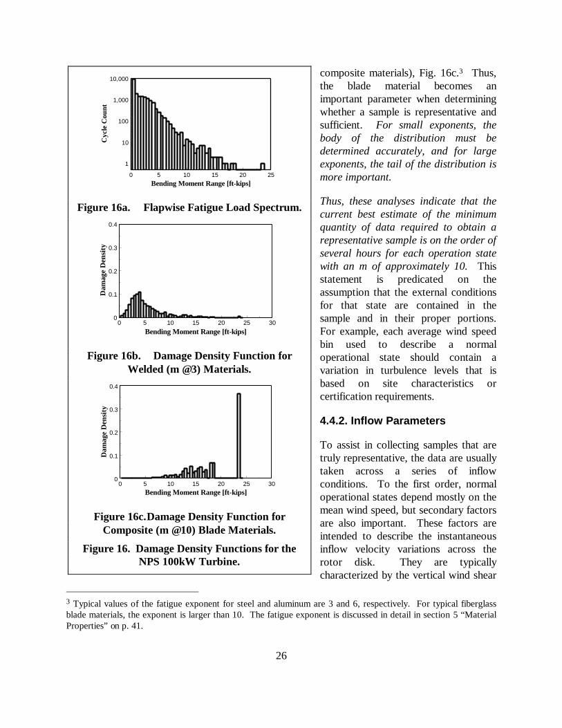
26

composite materials), Fig. 16c.3 Thus,the blade material becomes animportant parameter when determiningwhether a sample is representative andsufficient. For small exponents, thebody of the distribution must bedetermined accurately, and for largeexponents, the tail of the distribution ismore important.

Thus, these analyses indicate that thecurrent best estimate of the minimumquantity of data required to obtain arepresentative sample is on the order ofseveral hours for each operation statewith an m of approximately 10. Thisstatement is predicated on theassumption that the external conditionsfor that state are contained in thesample and in their proper portions.For example, each average wind speedbin used to describe a normaloperational state should contain avariation in turbulence levels that isbased on site characteristics orcertification requirements.

4.4.2. Inflow Parameters

To assist in collecting samples that aretruly representative, the data are usuallytaken across a series of inflowconditions. To the first order, normaloperational states depend mostly on themean wind speed, but secondary factorsare also important. These factors areintended to describe the instantaneousinflow velocity variations across therotor disk. They are typicallycharacterized by the vertical wind shear

3 Typical values of the fatigue exponent for steel and aluminum are 3 and 6, respectively. For typical fiberglassblade materials, the exponent is larger than 10. The fatigue exponent is discussed in detail in section 5 “MaterialProperties” on p. 41.

0 5 10 15 20 25

1

10

100

1,000

10,000

Bending Moment Range [ft-kips]

Cyc

le C

ount

Figure 16a. Flapwise Fatigue Load Spectrum.

0 5 10 15 20 25 300

0.1

0.2

0.3

0.4


Dam

age

Den

sity

Figure 16b. Damage Density Function forWelded (m ≅ 3) Materials.

0 5 10 15 20 25 300

0.1

0.2

0.3

0.4


Dam

age

Den

sity

Figure 16c.Damage Density Function forComposite (m ≅ 10) Blade Materials.

Figure 16. Damage Density Functions for theNPS 100kW Turbine.

27

across the rotor and the single-point turbulence intensity measured at hub-height in front of theturbine. Although these parameters are typically the only ones specified in the certificationprocess, several other parameters have been proposed for characterizing the inflow across therotor. These parameters warrant consideration when defining a representative sample for all ofthe inflow conditions from short-term average inflow velocity data. Sets of parameters that havebeen proposed for defining the inflow are discussed in section 6.2 “Inflow Characteristics” on p.76.

In another approach to the problem, Kashef and Winterstein [59] have demonstrated that thedependence of the blade loads on mean wind speed and turbulence may be reduced to a singlevariable that is based on the standard deviation of the high-frequency turbulence. Namely, whenthe low-frequency components (well below the rotor speed) of the inflow velocity u are removed,the resulting turbulence level $uH can be correlated to the distribution of fatigue cycles across allmean inflow velocities. The initial evaluation of this correlation was based on data from a singleturbine. When extended to another, smaller data set, the correlation to $uH broke down and wasreplaced by a dependence on the average inflow velocity U.

The crux of the analyses summarized here, as pointed out by Kashef and Winterstein [59], is thatthe correlation between fatigue loads and inflow parameters is probably case dependent. At thistime, the appropriate distribution of inflow parameter(s) across a cycle count bin has not beenidentified. The IEC Standards Committee, [17, 22] recommends that the turbulence intensity, asa function of average inflow velocity, should be the governing parameter for describing the inflowfor design load calculations. The IEC recommendations define this functional relationship.Implicit to this formulation is that the turbulence intensity will be a constant across a cycle countbin. My view is that this approach is somewhat simplistic and that the fatigue load spectrumshould use, at the very least, a distribution of turbulence intensities across each cycle count bin.

From an analysis standpoint, the inflow is typically described using the SNLWIND model [63-65].In this model, the mean inflow velocity, the integral length scale, and the shear velocity (related tothe turbulence $u ) are typical input parameters for the turbulence and coherence modeling of theinflow. Thus, additional variations in length scales and/or the Reynolds stresses [particularly the

¢¢u wb g term] are warranted when defining the inflow distributions across a particular cycle countbin; see the detailed discussion of inflow parameters in section 6.2 “Inflow Characteristics” on p.76.

Cuerva-Tejero et al. [66] have suggested yet another approach to solving this difficult problem.They used “principal component” and regression analysis to identify combinations of inflowparameters to develop a set of four factors that describe the inflow. In general, these four factorsmay be associated with various parings of the common inflow parameters. One factor isassociated with the mean wind speed; the second with the high-level statistics of the wind speed(skewness and kurtosis); and the third and fourth with the stochastic characteristics of the windspeed (combinations of a length scale, a correlation coefficient and the standard deviations of itsthree components), and the fourth is turbulence and the correlation between the horizontalcomponent and the vertical component).

28

As discussed here, many parameters have been suggested as descriptors for the inflow. Whichdescriptors are necessary and sufficient remain to be determined.

4.4.3. Scaling and Extrapolating Representative Samples

Once the representative sample of the loads has been determined, the sample must be scaled intime to lifetime loads. Several techniques are currently used to scale them. Many designerssimply scale the sample loads directly. For normal operation, this scaling is typically based on theaverage annual wind speed distribution discussed in section 6.2 “Inflow Characteristics” on p. 76.These designers note that the samples define the main body of the load distribution, and thus, theycapture all of the necessary loads on the turbine to define its service lifetime.

Other designers note that the infrequent occurrences of high-stress events contained in the “tail ofthe load distribution” are affected by the specific data set, and that the distribution tails fill in asmore and more data are added to the record [47, 67]. And, as noted above, the existence of a“high stress tail” on the distribution has significant influence on the predicted service lifetime ofthe turbine. Thus, they believe that it must be well defined for an accurate analysis. This group ofdesigners typically extrapolates from the body of the cycle count distribution into this tail region.

As discussed by Lange and Winterstein [58], the data contained in a representative sample definesthe main body of the load distribution on the turbine very well. However, the extreme loads in thehigh-stress tail of the distribution may or may not be defined accurately. In section 4.3“Analytical Descriptions of Normal-Operation Load Spectra” on p. 18, curve-fitting techniquesare used to develop analytical descriptions of the load distribution. These fits may also be used toextrapolate limited data to the prediction of the tail of the load distribution. Thus, statisticalmeasures of the data are potentially very useful for deducing the shape and magnitude of the low-probability-of-occurrence, high-stress tail of the load distribution.

There are two critical issues for this technique. The first concerns the use of statistical modelingto deduce the shape and magnitude of the low-probability-of-occurrence, high-stress tail of theload distribution and the second concerns the extent of the predicted tail that is realized during thelife of the turbine.

For the latter, the argument is that under a probabilistic framework, large loads are possible, butthey are associated with a decreasing rate-of-occurrence (i.e., large return period or a decreasingexceedence probability). Hence they may quickly become irrelevant in practical applications, suchas wind turbines with a finite service lifetime. While these large-load cycles may truly have a finiteprobability of occurrence, their existence is controversial and typically difficult to estimate fromdata. Several researchers have questioned the realism of the prediction in the tail of thedistribution [55]. Their skepticism is based on the realization that the relatively smallrepresentative sample is to be extrapolated to a 30-year lifetime. Consider the case where eachwind speed bin contains only a single 10-minute record. For an 8 m/s Raleigh site (see thediscussion in section 6.1 “Annual Average Wind Speed” on p. 75), the turbine will operateapproximately 5.5 percent of the time in the 11-12 m/s wind speed bin. Thus, the extrapolationtechnique is being asked to extend the data from the 1 per 10 minutes fractal to the 1 per 1.65

29

year fractal (5.5 percent of 30 years); i.e., by a factor of approximately 90 thousand(0.055x30x365x24x6)! Even if an hour of data is used in each bin, the extrapolation will bealmost 15 thousand.

The discussion on the existence and extent of this high stress tail is very important because, asnoted above, the tail of the distribution is critical to the prediction of service lifetimes forcomposite turbine blades. Most designers fit the data with a distribution. In some cases, thedesigner will use the entire predicted distribution while others will truncate the distribution at fiveor ten times its RMS value (2nd moment of the distribution). However, at this time, there is noconsensus concerning the use of statistical models for predicting the shape and the extent of thetail of the load distribution used in service lifetime predictions. For conservative predictions, adistribution should be fit to the available data and used to extrapolate these data to long servicelifetimes. And, in no case should the distribution be truncated below the maximum measured orsimulated load level.

4.5. General Topics

4.5.1. Load Spectra Derived from Inflow Parameters

The analytical formulations cited in the previous section are descriptive models. Namely, they usemeasured loads data at a given set of inflow conditions and operational parameters to obtainmathematical formulations that describe the loads on the turbine. As discussed by Kashef andWinterstein [59], the correlation between fatigue loads and inflow parameters is probably casedependent, because each turbine will react to a turbulent inflow spectrum based on suchparameters as its size, architecture, modal frequencies, and damping characteristics. Thus, thedescriptive nature of these models implies that they are turbine and site specific.

A number of techniques have been proposed for extending the description of a turbine at one siteto another site or to another turbine. Jackson [68] offers a classical route to the extension ofthese formulations from descriptive models to predictive models. In this analysis, dimensionalanalysis is used to scale the size of the turbine. In another technique, Kashef and Winterstein [59]use a de-trending analysis to change sites. Spera [69] uses empirical relationships, derived fromrotationally-sampled inflow data, to obtain fatigue loads from structural analysis codes. And, inyet another approach developed by Kelley [49] and by Barnard and Wendell [70], the inflow timeseries is rainflow counted. The inflow cycles are then related to the fatigue cycles using a transferfunction. They postulate that the transfer function is constant for a given turbine.

4.5.2. Structural Analyses

The only true prescriptive models that can be used to analyze the fatigue loads, withoutexperimental measurements, are based on analytical inflow and structural analysis codes [25, 26].In this technique, an inflow model is combined with atmospheric design specifications and withaerodynamic load and structural analysis models to prescribe the fatigue loads on the turbine [24].The SNLWIND model, proposed by Veers [63, 64] and upgraded to three components by Kelley[49, 65], is typically used in the U.S. The European models are typified by the work of Mann

30

[71]. Popular aero/structural codes used in the U.S. are the analyses by Wilson et al. using theFAST code [72], Hansen using the YawDyn code [73], and Elliott and Wright using theAdams/WT code [74]. Detailed discussions of these codes are beyond the scope of this report.Quarton [75] provides a detailed summary of wind turbine design analysis.

The direct application of the structural analysis codes for predicting of fatigue loads is beyond thescope of this report and will not be discussed here. Direct ties between structural analysis codesand fatigue analysis have been conducted by Wilson et al., [76] for the FAST code and Laino andHansen [77-79] for the YawDyn and Adams/WT codes.

4.5.3. Bin Size

Binsing rainflow cycle counts into count matrices is typically the technique of choice for analyzingthe cyclic loads on a wind turbine. However, the accuracy of this technique is limited by the sizeof bins. In particular, the cycle counts within a bin are spread across the bin. Because the damagecontained within the bin, see Eq. 5, is a non-linear function of its stress level, the characterizationof all the load cycles within a bin at a single level can significantly under or overestimate theirdamage to the structure. Several analytical techniques, based on materials properties and on theassumed distribution of the loads contained in the bin, can locate the damage centroid for the bin.However, these techniques are typically overkill. A conservative technique is to use the higheststress level for each bin as stress level for all cycles in that bin and to keep the size of each binrelatively small. For the latter, the minimum recommended number of bins is fifty [25], and theexpected maximum cyclic stress is typically set to fall within the 70 percent bin.4

4.5.4. Mean Value Bins

As discussed above, the fatigue load spectrum may be described using one of threerepresentations: the range spectra in a column of cycle counts, a range and mean spectra in a 2-Dmatrix of cycle counts, and a Markov matrix of peaks and valleys in a from-to matrix. The range-mean (2-D) cycle-count matrix is the form favored by this author for most applications. Theinclusion of the mean value in the description of each cycle count adds important informationconcerning the general state of stress (strain) on the component. This information can be usedeffectively by the linear damage models and the additional information is gained with littleadditional complexity.

However, this view is not shared by all. In reduced formulations (2-D to 1-D), the variation ofthe mean stress across cycles is replaced by a single average value in some fitting techniques and,in others, the variation is totally ignored. In an apparent contradiction to the statement in thepreceding paragraph, the author has used several of the reduced formulations extensively, e.g., seesection 4.3.3 “Generalized Curve Fitting Techniques” on p. 20. The use of a reduced formulation

4 The purpose of the 70 percent value is to provide room-at-the-top of the cycle count matrix; in particular, if anunexpectedly high stress cycle occurs, it will be included accurately in the cycle count matrix. If data arepreprocessed, the 70 percent value may be increased to reflect the known value of the highest stress cycle.

31

is supported by several observations. For most turbine load spectra, the range of mean stresses isrelatively small. And, if the material properties are based on a mean stress or an R value that fallssomewhere near the middle of this range, service lifetime predictions are typically close to thosepredicted using the mean stress information.5 Thus, the variation of the cycle counts with meanstress can sometimes be ignored if the material properties used in their evaluation are based onan average mean value. However, designers should evaluate their designs and load spectra usingboth techniques before using one or the other, to ensure that their choice does not lead to a non-conservative estimate of the service lifetime.

4.5.5. Counting Cycles

As discussed above, the data samples forming the representative data set are formulated fromrelatively short samples of data that are collectively on the order of several hours in duration.Typically, the duration of each segment is 10 minutes. These segments are counted as series ofindependent segments or concatenated into a single file for counting. As pointed out in Kelleyand Sutherland [62] and Mouzakis and Morfiadakis [80], the two techniques can producesignificantly different servicelifetime predictions because thecloseout cycles may not bematched correctly and the low-occurrence cycles may bemissed entirely. Mouzakis andMorfiadakis [80] demonstratethat the service lifetimepredictions based on segmenteddata can underestimate damageby over 40 percent for materialswith large fatigue exponents.For smaller material exponents,the effects are less dramatic.Using time-series data that wasdivided into 10-minutesegments, they comparedpredicted service lifetimes withand without closeout and low-occurrence cycles. Their results are shown in Fig. 17. For thisfigure, the time-series data were counted first in segments without closing the half-cycles. Theresulting damage calculation yielded the reference service lifetime. The data were then re-countedin segments with the half cycles included in the count. The resulting service lifetime is comparedto the reference service lifetime in the plots labeled “Half Cycles” in the figure. The data wererecounted a final time with all of the time-series data concatenated into a single file. Half cycles

5 As discussed in detail below, the fatigue properties of typical wind turbine materials are significantly moredependent on the alternating stress level than on the mean stress level.

2 4 6 8 10 12 140

20

40

60

80

100

Material Fatigue Exponent

Life

time

Red

uctio

n, p

erce

nt

Flatwise:ConcatenatedHalf Cycles

Edgewise:ConcatenatedHalf Cycles

Figure 17. Effect of Segmented Data on the Predictionof Service Lifetimes.

32

were included in this count as well. This resulting damage yielded plots labeled “Concatenated” inthe figure. Thus, when the representative data set is segmented, the sets should be counted as asingle, continuous record. This discussion is continued in section 4.6.2 “Transition Cycles” on p.33 where the cycles between operational states are discussed.

4.5.6. Equivalent Fatigue Load

To describe the impact on fatigue from a spectral load distribution, the concept of an equivalentfatigue load may be used [31]. In general, the equivalent fatigue load is determined using Miner’sRule (see Eqs. 5 through 7) to determine a single, constant-rate fatigue load that will produceequivalent damage. If the equivalent cyclic load F(•) has a mean stress level of (σm)e, and analternating level of (σa)e, then:

F s ss s

s ss s s sm e a e

m e a e

m a

m aa m

,

N , =

n , N ,

d db g b gb g b g

b gb gvwf0

0

•

- •

•

, (25)

where fo is the cyclic rate for F(•) and N(•) is the number of cycles to failure at the specified meanand alternating stress level, see Eq. 9. In the absence of actual cycle counts, the frequency fo maybe taken to be 1 p (i.e., the blade rotation rate) for the edgewise bending moments and 3 p forflapwise bending moments of three-bladed machines and 2 p for two-bladed machines. F(•) is notunique. Typically, the mean value (σm)e is chosen and then (σa)e is calculated.

Obviously, this equivalent fatigue load is material dependent. As discussed in section 5 “MaterialProperties” starting on p. 41, this formulation may take one of several forms. For power lawformulations, see Eq. 31, with a constant mean stress, Eq. 25 may be written in the form:

ss

a e

am

ii

1m

= n

T b g

b gÂL

NMMM

O

QPPPf0

, (26)

where m is the fatigue exponent, and T is the total time covered by the load spectrum. Typicalvalues for m are 3 for welded steel, 6 for extruded aluminum and 10 for fiberglass compositematerials.

The equivalent fatigue load is one method used to test wind turbine components in fatigue [81].In this simulation technique, the spectral loads on a component are replaced with a constantamplitude load cycle. This technique for simulating spectral loads significantly simplifies theexperiment. Moreover, by increasing the amplitude of the equivalent fatigue load (mean and/oralternating stress level), the service lifetime of the component can be simulated in a relatively shorttime period. However, these simulations are predicated on the validity of the assumed damagelaw and a detailed understanding of material behavior.

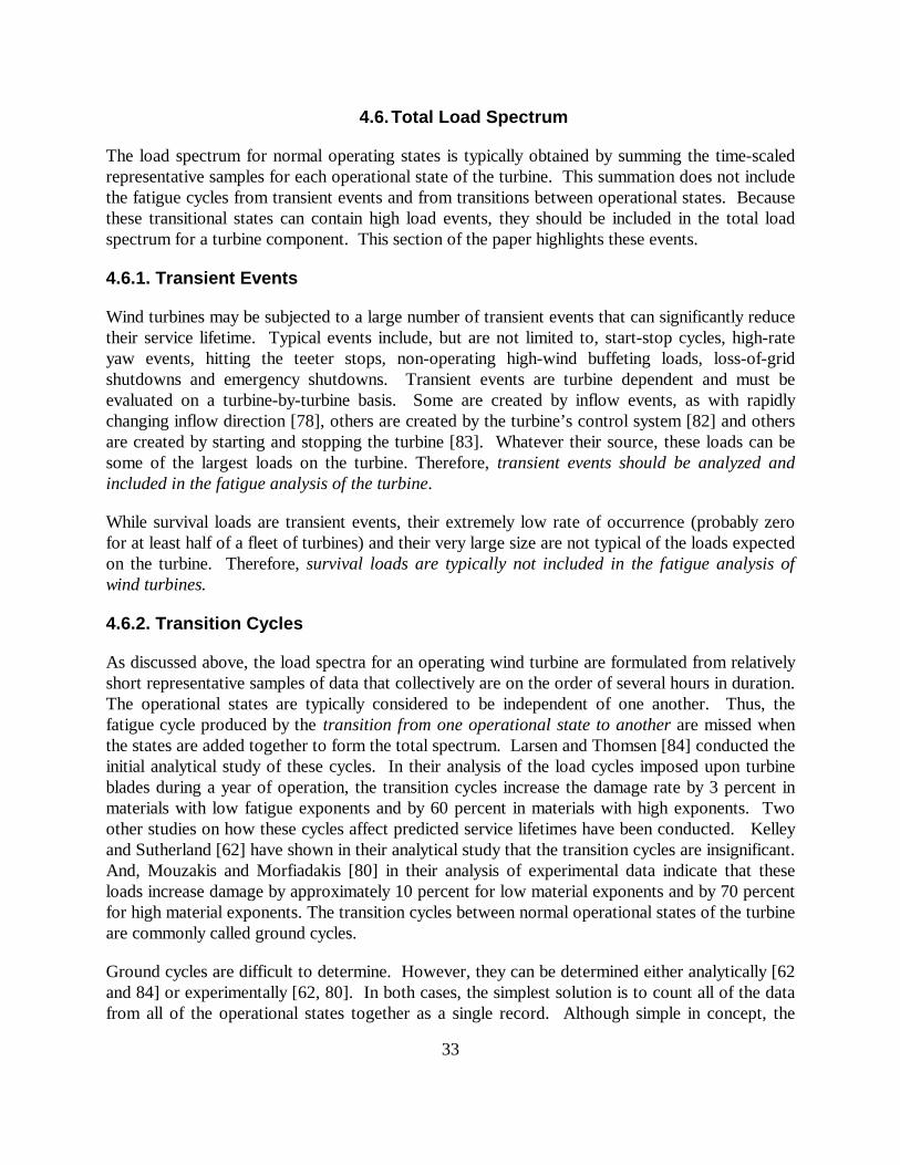
33

4.6. Total Load Spectrum

The load spectrum for normal operating states is typically obtained by summing the time-scaledrepresentative samples for each operational state of the turbine. This summation does not includethe fatigue cycles from transient events and from transitions between operational states. Becausethese transitional states can contain high load events, they should be included in the total loadspectrum for a turbine component. This section of the paper highlights these events.

4.6.1. Transient Events

Wind turbines may be subjected to a large number of transient events that can significantly reducetheir service lifetime. Typical events include, but are not limited to, start-stop cycles, high-rateyaw events, hitting the teeter stops, non-operating high-wind buffeting loads, loss-of-gridshutdowns and emergency shutdowns. Transient events are turbine dependent and must beevaluated on a turbine-by-turbine basis. Some are created by inflow events, as with rapidlychanging inflow direction [78], others are created by the turbine’s control system [82] and othersare created by starting and stopping the turbine [83]. Whatever their source, these loads can besome of the largest loads on the turbine. Therefore, transient events should be analyzed andincluded in the fatigue analysis of the turbine.

While survival loads are transient events, their extremely low rate of occurrence (probably zerofor at least half of a fleet of turbines) and their very large size are not typical of the loads expectedon the turbine. Therefore, survival loads are typically not included in the fatigue analysis ofwind turbines.

4.6.2. Transition Cycles

As discussed above, the load spectra for an operating wind turbine are formulated from relativelyshort representative samples of data that collectively are on the order of several hours in duration.The operational states are typically considered to be independent of one another. Thus, thefatigue cycle produced by the transition from one operational state to another are missed whenthe states are added together to form the total spectrum. Larsen and Thomsen [84] conducted theinitial analytical study of these cycles. In their analysis of the load cycles imposed upon turbineblades during a year of operation, the transition cycles increase the damage rate by 3 percent inmaterials with low fatigue exponents and by 60 percent in materials with high exponents. Twoother studies on how these cycles affect predicted service lifetimes have been conducted. Kelleyand Sutherland [62] have shown in their analytical study that the transition cycles are insignificant.And, Mouzakis and Morfiadakis [80] in their analysis of experimental data indicate that theseloads increase damage by approximately 10 percent for low material exponents and by 70 percentfor high material exponents. The transition cycles between normal operational states of the turbineare commonly called ground cycles.

Ground cycles are difficult to determine. However, they can be determined either analytically [62and 84] or experimentally [62, 80]. In both cases, the simplest solution is to count all of the datafrom all of the operational states together as a single record. Although simple in concept, the

34

technique is very difficult in practice because a large amount of data must be analyzed. Moreover,each sample must be added in proportion to its expected probability of occurrence and in itsexpected sequence. Larsen and Thomsen [84] have actually conducted such a simulation. In theirtechnique, the load spectrum for the transition between operational states is predicted analytically,then long-term inflow simulations are used to predict the number of transitions between each andevery two states for the life of the turbine. Their results are cited above.

Thus, if ground-cycle data are available, they should be used in the service lifetime analysis.However, because these data are difficult to obtain and predictions of service lifetimes are, atmost, only marginally affected by them, we conclude that that ground cycles may be ignored inmost service lifetime predictions.

4.6.3. Comment

While differences of 10 percent and 70 percent variation in the predicted service lifetimes seemhigh, one should remember that for many applications, uncertainties in the loads, materials anddamage typically yield widely varying damage predictions. For wind turbine applications,differences of a factor of 2 between damage predictions and measured lifetimes are not onlycommon, they should be expected. Once said, there are several places were these relatively smalluncertainties occur, see above and below. Unfortunately, most are non-conservative and they canadd to a significant result. Thus, the designer should include as many of these special-case fatigueloads in the design calculations as practically possible.

4.6.4. Summation of Load States

Once the representative samples of the load spectra have been assembled, they must be summedto estimate the lifetime of the turbine. As indicated in Eq. 11, the normal operation cyclic loadsare weighted using the annual wind speed distribution and then summed to find the total operatingload spectrum. The number of significant transient events is projected and then added to theoperating spectrum. The result is the total load spectrum on the wind turbine.

4.6.5. Partial Safety Factors

To assure a safe design, the IEC-61400-1 standard [17] uses partial safety factors to cover theuncertainties and variabilities in the loads (and in the materials). Namely, the partial safety factorsaccount for the possibility of unfavorable deviations of the load from the characteristic value andfor uncertainties in the loading model. A discussion of partial safety factors and their applicationto wind turbine design is beyond the scope of this report and will not be discussed here.

4.7. Off-Axis Analysis

In most wind turbine blade analyses and experimental data sets, the loads are decomposed intotwo primary bending moments along the primary blade axes. The first primary moment, called the“flap” or “flatwise” bending moment, is bending out of the plane of rotation. The second, called

35

the “edgewise” or “lead-lag” bending moment, is bending in the plane of rotation.6 In the initialdiscussions here, these loads are treated independently. However, the critical fatigue loads (stresscycles) imposed on the blade may not be along one of these primary blade axes [85, 86]. Rather,the critical loads may occur along another axis. Sutherland [85] has presented both time-domainand frequency-domain analysis techniques for determining the off-axis fatigue cycles fromprimary-axis loads.

4.7.1. Geometric Load Parameters

To determine the off-axis stress states in a blade section, the two principal bending stresses at thatblade station may be added together vectorially, see Timoshenko [87]. Combining the stressesyields:

sq r s q r s q( ) ( ) cos( ) ( ) sin( )t F t E t= +F E , (27)

where σθ is the bending stress at time t and angle θ, σF is the root flapwise bending stress, σE isthe root edgewise bending stress, and rF and rE are geometric correction factors. The angle θ isdefined here to be the angle from the positive edgewise bending principal (neutral) axis toward thenegative flapwise bending principal axis; i.e.,from the tension side of the flapwise bendingmoment to the tension side of the edgewisebending moment, see Fig. 18. For time-seriesdata, the time t in Eq. 27 is simply replaced bytj, namely the jth component of the time series.The geometric factors rF and rE adjust thebending stress at the outer fibers of theprincipal axes to the bending stress at the outerfibers at the angle θ. The values for rF and rEare determined from:

= y

y

= y

y

Fo

o F

Eo

o E

r

r

qq

qq

b g b gb g

b g b gb g

, (28)

where (yo)θ is the distance from the intersection of the principal axes to the outer fibers at angle θ,and (yo)F and (yo)E are the distances from the principal axis to the outer fibers along the flapwiseand the edgewise axes, respectively, see Fig. 18.

6 These definitions are not universal. For turbines with coned and/or pitch blades, the definitions of flapwise andedgewise bending moments are typically modified to be perpendicular and parallel to the chord line of the blade.

(y )o F

θ

Edgewise BendingNeutral Axis

Flapwise BendingNeutral Axis

o E(y )(y )

o θ

Figure 18. Geometric Parameters for anElliptical Root Section.

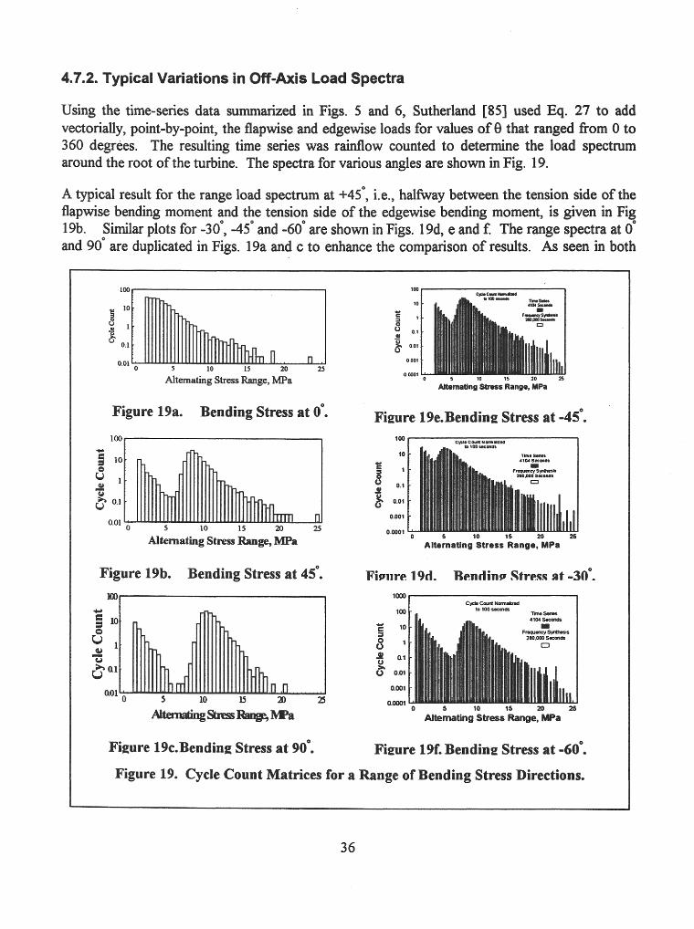
4.7.2. Typical Variations in OfF-Axis Load Spectra

Using the time-series data summarized in Figs. 5 and 6, Sutherland [85] used Eq. 27 to add vectorially, point-by-point, the flapwise and edgewise loads for values of 6 that ranged from 0 to 360 degrees. The resulting time series was raintlow counted to determine the load SpectNm around the root of the turbine. The spectra for various angles are shown in Fig. 19.

A typical result for the range load spectrum at +45', i.e., halfway between the tension side of the flapwise bending moment and the tension side of the edgewise bending moment, is given in Fig 19b. Similar plots for -3Oq -45' and -60' are shown in Figs. 19d, e and f. The range spectra at 0' and 90" are duplicated in Figs. 19a and c to enhance the comparison of results. As seen in both

Alternating Stress Rsnge, Mpa

Figure 19a. Bending Stress at 0'.


Figure 19b. Bending Stress at 45*.

--I

Altatlatinp-mm

Figure 19c.Bending Stress at 90'.

Ahmating Stmss Range. Y R

Figure 19cBendine Stress at -45'.

Altematinp Stress Range. MPa

Fiviire 19d. Rendin9 Strew at -30'.

memating Stress Flmnge,MPa

Fieure 19f. Bending Stress at -60'.

Figure 19. Cycle Count Matrices for a Range of Bending Stress Directions.

36

37

figures, the typical two-hump characteristic of the edgewise-bending stress is still strong in all ofthe off-axis spectra. These plots are based on a frequency domain analysis proposed bySutherland [85].

4.8. Specialized Load Spectra for Testing

4.8.1. Variable Amplitude Test Spectrum

The bulk of the fatigue testing of materials and wind turbine components is constant amplitudetesting over a large variety of both compressive and tensile loads. However, wind turbines aresubjected to a spectrum of loads that can significantly change their behavior; see the discussion byVeers et al. [30]. Thus, constant amplitude testing may not be characterizing their fatigueresponse correctly.

To determine if constant amplitude tests can be used to predict the service lifetimes of turbinecomponents under spectral loading, specimens must be tested under spectral loads that arerepresentative of the loads on the turbine. The European community was the first to develop atest-load spectrum for wind turbine components. This spectrum is called WISPER (WInd turbinereference SPEctRum) for short [88, 89]. It was designed to represent the loads on a genericturbine operating alone in flat terrain. Because the loads in these conditions are relatively mildwhen compared to the spectrum imposed on a wind farm turbine in mountainous terrain, a secondtest spectrum, the U.S. Wind Farm spectrum, was proposed by Kelley [90]. This sectiondiscusses these two variable-amplitude test spectra.

4.8.1.1. WISPER

The WISPER reference-loading spectrum was developed by an international working groupcomposed of thirteen different European research institutes and manufacturers [88]. Theobjective of the effort was to specify variable-amplitude test-loading histories that model rootflapwise (out-of-plane) bending of horizontal-axis wind turbine blades in the field. These featuresinclude exhibiting a spectral shape that is characteristic of the type of structure under test, whilealso providing the interactions thought to be important in such a stochastic environment. Greatcare was taken to ensure that the final loading spectra did not represent any particular turbinedesign or operating environment (e.g., the WISPER loads are not time correlated). Thesefeatures imply that this test-load spectrum is to be used for comparative purposes only.

WISPER is derived from eight load cases that are called classes or modes. The first two classesare the loads for discrete events, specifically turbine start-up (Class 1) and stopping (Class 2).The six remaining classes, 3 through 8, are based upon 10-minute load histories obtained duringcontinuous operation of the turbines over their operating wind speed range. Mode 3 containsrepresentative data for mean wind speeds below 9 m/s. Modes 4 through 7 contain data for meanwind speeds of 9-11, 11-13, 13-15, and 15-17 m/s, respectively. Finally, Mode 8 describes theloads for mean wind speeds exceeding 17 m/s.

38

The loads in WISPER are based on a large population of load measurements from nine two-bladed and three-bladed turbines. Their rotor diameters ranged from 11.7 to 80 m. A total of 65rainflow counted load cycle matrices (sorted by WISPER Wind Speed Class) were used toconstruct the WISPER spectrum. For Modes 3-8, the individual matrices from each turbine werenormalized by the magnitude of the load cycle occurring once per 1000 revolutions. Thenormalized matrices for each wind speed class were then averaged together to reduce theinfluence of individual turbines. Using this approach, six normalized load cycle matrices wereobtained; one each for Wind Speed Classes 3 through 8. The normalization of Operating Modes1 and 2 (start-up/stop) was handled somewhat differently. A detailed discussion of this procedureis not warranted here.

The WISPER protocol uses the six normalized load spectra as representative samples for theoperation of the turbine. The total load spectrum is obtained by adding each of theserepresentative samples together in proportion to the number of hours the turbine will operateduring a two-month period. The hours of operation used in the WISPER protocol are based onthe long-term wind statistics from two different sites along the northern coast of Germany.

While WISPER offers the complete range of loads on a wind turbine (approximately 130,000 loadcycles), researchers have found that its many small load cycles make testing somewhat difficult.To provide a shorter testing sequence, the low-amplitude cycles have been removed from theWISPER load spectrum to form the WISPERX load spectrum. The latter reduces the number ofload cycles by approximately a factor of 10 (approximately 13,000 load cycles remain) byremoving all cycles with an amplitude of level 17 or less (WISPER has a total of 64 load levels).WISPERX maintains all of the larger cycles in both tension and compression. For testing rates of2 Hz, a WISPERX test block will require approximately 2 hours to complete, while a WISPERtest block will require about 18 hours.

4.8.1.2. U.S. Wind Farm Spectrum

The U.S. wind farm spectrum was developed by Kelley [90] based on operating data obtainedfrom two Micon 65 turbines that were tested at Row 37 of a 41-row wind farm in San GorgonioPass, California [91, 92]. The data set consisted of 397 10-minute records that were collectedover a wide range of inflow conditions during the late wind season (late July and early August).These data were processed using the WISPER development protocol to form the load cyclematrices for Modes 3 through 7.

The U.S. wind farm spectrum does not compare directly with the WISPER spectrum because theyare based on different wind speed distributions. To provide a comparison, the normalized loadcycle matrices from the WISPER spectrum were combined with the San Gorgonio wind speeddistribution to form an equivalent WISPER spectrum for the San Gorgonio site. The equivalentWISPER distribution is compared to the U.S. wind farm spectrum in Figure 20. As shown in thisfigure, the San Gorgonio spectrum has many more cycles than does WISPER. And as verified bySutherland and Kelley [93], the former is significantly more damaging.

39

4.8.2. Load Spectra for Gears

The conventional design technique used for a non-wind generator gearbox is based on themaximum torque transmitted through the box and by the spectral content of the operational loads.The spectral content is usually characterized by a service factor. Recommended service factorsfor normal applications are supplied by gearbox manufactures and standardized by the AmericanGear Manufacturers Association (AGMA). For example, a service factor of 1.0 is recommendedfor relatively short duration applications involving uniform loads, as with rotary pumps for liquids.A factor of 2.0 is recommended for continuousapplications involving reciprocating loads, aswith cooling tower fans or beet slicers in thesugar industry. Unfortunately, the uniquetorque spectrum imposed upon gearboxes usedin wind turbines precludes designs based uponany of the standard categories.

In a technique that is used to characterize andanalyze the loads on a typical wind turbinegearbox, McNiff et al. [83] developed a “time-at-level” histogram for the loads on thegearbox. In this technique, the torque appliedto the gearbox is characterized by the total timethe gearbox will be subjected to a givenmagnitude of torque. Figure 21 presents theannual time-at-level histogram developed by

10 20 30 40 501E+0

1E+1

1E+2

1E+3

1E+4

1E+5

1E+6

Bending Moment, kNm

Cum

ulat

ive

Cyc

les

Whisper Spectrum

Wind Farm Spectrum

Figure 20. Cumulative 2-Month Reference Alternating Load Spectrum.

-20 -15 -10 -5 00

200

400

600

Low Speed Shaft Torque, kN-m

Ann

ual H

ours

High Turbulence Data

Low Turbulence Data

Figure 21. High and Low TurbulenceTorque Spectrum for the Micon 65.

40

McNiff, Musial and Errichello [83] for theMicon 65 turbine. The development of theseloads is based on a point-by-point binsing ofthe time series data by magnitude. Theservice lifetime analysis assumes that eachtorque bin is applied to the gearbox in a quasi-static manner; namely, the torque is a slowlyvarying function of time.7 Thomsen andPetersen [94] conducted a similar study forboth stall and pitch controlled wind turbines.

In the time-at-level technique, the torque timeseries is binsed by magnitude. The number ofstress cycles on an average gear tooth isdetermined from this histogram by dividingthe time in each torque bin by the duration ofa tooth engagement (or, conversely, multiplyby the rate of tooth engagement) and, thendividing by the number of teeth on the gear.Thus, the cycle count histograms and thetime-at-torque histograms are simple multiplesof one another.

The time-at-torque histogram for a Micon65 turbine is shown in Fig. 22. As shown inthis figure, the time-at-torque is a function ofsample rate. Sutherland and Burwinkle [95]have demonstrated that the time-at-torquetechniques yield essentially equivalent resultsto rainflow counting the tooth loads; namely,for the fatigue analysis of gears, torque loadsmay be considered to be slowly varyingfunctions of time.

A joint AGMA (American Gear Manufactures Association) and AWEA (American Wind EnergyAssociation) committee has developed design guidelines for gearboxes used in wind turbineapplications [96].

7 A “slowly varying function of time” implies that the torque loads on the gear teeth produce a single stress cycleper each tooth engagement.

5. 10 15 20.0

5

10

15

20

Shaft Torque, kN-m

Tim

e at

Tor

que,

sec Sample Rate

32 Hz

7.5 Hz

1 RPM

Micon 65

Normalized to100 sec

Record Length600 secAverage Wind Speed13.5 m/s

Figure22a. Linear Histogram.

2 2.2 2.4 2.6 2.8 30.01

0.02

0.05

0.1

0.2

0.5

1

2

5

10


-Ln(

1-C

DF)

Sample Rate

32 Hz

1 rpm

Micon 65Normalized to100 sec

Record Length600 secAverage Wind Speed13.5 m/s

Figure 22b. Weibull Plot.

Figure 22. Time-at-Torque Histogram forthe Micon 65.

41

5. MATERIAL PROPERTIES

Most of the materials used in theconstruction of wind turbines aretypical of those materials that areused in rotating machinery andtowers. Thus, the turbine systemis primarily composed of materialsthat are relatively commonstructural materials with extensiveengineering applications anddatabases. However, blades areunique structural components ofwind turbines. They are aminimum weight and costcomponent that must endure a verylarge number of fatigue cyclesduring their service lifetime. Asshown in Fig. 23, blades mustendure several orders of magnitude more cycles than an airplane, the original fatigue criticalstructure. Thus, turbine blades are also fatigue critical structures. Moreover, the cost of thematerials used in the turbine must be kept at a relative minimum to ensure a commercially viableproduct.

Wind turbine blades have been made from a variety of materials that range from wood to metalsto composites. Wood (a naturally occurring composite material) has proven to be a successfulmaterial. Its relatively high strength-to-weight ratio, and good stiffness and resilience yield highquality blades. Wood was used in the early windmills (including the early Dutch windmills and theU.S. water pumpers) and has remained a favorite with the designer of small and medium sizedwind turbines. However, wood’s inherent problems with moisture stability and joining efficiency[97] have forced designers to examine other materials. Metals were initially a popular materialbecause they yield a low-cost blade and can be manufactured with a high degree of reliability.However, most metallic blades (steel) proved to be relatively heavy, which limits their applicationin commercial turbines. Lightweight metals (aluminum) have found some applications.Composites have become the blade material of choice. High strength and stiffness and the abilityto tailor the material to the loads has led to its widespread use as a blade material.

The bulk of the fatigue properties developed for materials that are used in wind turbinecomponents are based on coupon tests conducted under constant amplitude loading. Thetechniques used in these tests have varied widely. Swanson [98] provides a general reference fortypical testing techniques. This section provides a general overview of the fatigue properties forthe various wind turbine blade materials and references to fatigue databases.

Cyc

lic S

tres

s

30 Year Design Life

Helicopter Design

5 6 7 8 109 11

Aircraft Design

Log10(Cycles to Failure)

Figure 23. Schematic S-N Diagram for VariousFatigue Critical Structures.

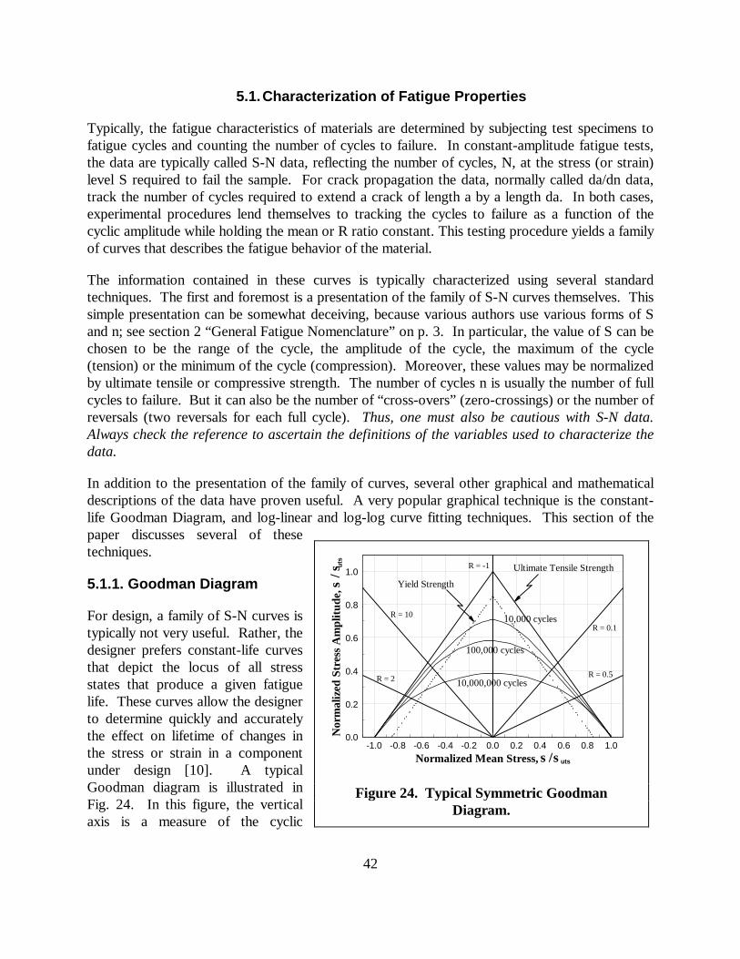
42

5.1. Characterization of Fatigue Properties

Typically, the fatigue characteristics of materials are determined by subjecting test specimens tofatigue cycles and counting the number of cycles to failure. In constant-amplitude fatigue tests,the data are typically called S-N data, reflecting the number of cycles, N, at the stress (or strain)level S required to fail the sample. For crack propagation the data, normally called da/dn data,track the number of cycles required to extend a crack of length a by a length da. In both cases,experimental procedures lend themselves to tracking the cycles to failure as a function of thecyclic amplitude while holding the mean or R ratio constant. This testing procedure yields a familyof curves that describes the fatigue behavior of the material.

The information contained in these curves is typically characterized using several standardtechniques. The first and foremost is a presentation of the family of S-N curves themselves. Thissimple presentation can be somewhat deceiving, because various authors use various forms of Sand n; see section 2 “General Fatigue Nomenclature” on p. 3. In particular, the value of S can bechosen to be the range of the cycle, the amplitude of the cycle, the maximum of the cycle(tension) or the minimum of the cycle (compression). Moreover, these values may be normalizedby ultimate tensile or compressive strength. The number of cycles n is usually the number of fullcycles to failure. But it can also be the number of “cross-overs” (zero-crossings) or the number ofreversals (two reversals for each full cycle). Thus, one must also be cautious with S-N data.Always check the reference to ascertain the definitions of the variables used to characterize thedata.

In addition to the presentation of the family of curves, several other graphical and mathematicaldescriptions of the data have proven useful. A very popular graphical technique is the constant-life Goodman Diagram, and log-linear and log-log curve fitting techniques. This section of thepaper discusses several of thesetechniques.

5.1.1. Goodman Diagram

For design, a family of S-N curves istypically not very useful. Rather, thedesigner prefers constant-life curvesthat depict the locus of all stressstates that produce a given fatiguelife. These curves allow the designerto determine quickly and accuratelythe effect on lifetime of changes inthe stress or strain in a componentunder design [10]. A typicalGoodman diagram is illustrated inFig. 24. In this figure, the verticalaxis is a measure of the cyclic

-1.0 -0.8 -0.6 -0.4 -0.2 0.0 0.2 0.4 0.6 0.8 1.00.0

0.2

0.4

0.6

0.8

1.0

Normalized Mean Stress,

Nor

mal

ized

Str

ess

Am

plitu

de,

R = 0.5

R = 0.1

R = -1

R = 2

utsσ/σ

R = 10

Ultimate Tensile Strengthuts

σ/σ

Yield Strength

10,000,000 cycles

10,000 cycles

100,000 cycles

Figure 24. Typical Symmetric GoodmanDiagram.

43

amplitude, and the horizontal axis is a measure of the mean stress. In both cases, theses stresslevels have been normalized by the ultimate tensile strength of the material.

Figure 24 illustrates that a constant R ratio plots as a straight line in this diagram. All constant Rratio plots have their origin at zero mean and zero amplitude. Fully reverse bending, R = -1, is thevertical axis; i.e., the mean stress is zero.

In this figure, the constant life curves are bounded by the ultimate tensile strength of the materialon the tensile side (right side) of the diagram. This stress level plots as a straight line between(0,1) and (1,0). Likewise, the ultimate compressive strength bounds the compressive side ofdiagram (left side). It plots between (0,1) and (-1,0). Similar straight lines are shown in thefigure for the tensile and compressive yield stress. In this illustration, we assumed that the tensileand compressive strengths are equal.

Three representative constant life diagrams are shown in this figure, at 10,000, 100,000 and10,000,000 cycles. Each constant-life plot can be constructed from a family of S-N curves.Depending on the data behind the plot, the constant-life curve may be straight-line segmentedcurve or a smooth fitted curve.

This diagram illustrated in Fig. 24 is called symmetric; namely the left side of the plot is the mirrorimage of the right side of the plot. Thus, for symmetric materials, the ultimate tensile andcompressive strength must be equal, and fatigue life is dependent on the absolute value of themean stress. For symmetric materials, only the right half of the full Goodman diagram is typicallyplotted. Metals are typically symmetric materials; fiberglass materials typically are not.

5.1.2. General Characterizations of Fatigue Behavior

5.1.2.1. Curve Fitting S-N Data

As discussed by many authors, the S-N behavior of composite materials at a constant R value istypically fit using one of two equations. The first is a power law of the form:

σ = CN = CN1/m 1/k , (29)

or alternately,

log logsb g b g b g = C +1m

log N , (30)

where N is the number of cycles to failure at stress level σ, and the coefficient m, sometimesdenoted by k or b, is called the fatigue exponent. In this form, the fatigue exponent is a negativenumber; i.e., the stress level decreases as the number of cycles increases. However, most fatigueliterature reports positive fatigue exponents; namely, Eqs. 29 and 30 have been rewritten with anexplicit negative sign. Thus, these two equations become:

44

s = CN = CN-1/m -1/k , (31)

log logsb g b g b g = C -1m

log N . (32)

In nondimensional form, Eq. 31 takes the form:

sso

-1/ m -1/k = C N = C N¢ ¢ , (33)

or

log logsso

= C -1m

log NFHG

IKJ ¢b g b g , (34)

where σo is the static strength of the composite. In this form, C' has a value of 1 when the curvefit to the S-N data set passes through the static strength at 100 cycles, i. e., at static failure in thefirst fatigue cycle. However, best fits for many materials yield values for C that are typically muchlarger than one. Thus, a multi-segmented curve is typically required to characterize the low andhigh cycle fatigue behavior of composites. For wind turbine applications where design lifetimesare relatively long, this region of the curve is typically not important.

The second form is given by a log-linear function of the form:

s = C -1m

log N = C - b log Nb g b g , (35)

or alternately,

10 = CN -1/ms , (36)

where the inverse of m is typically denoted by b. In nondimensional form, Eq. 35 takes thefollowing form:

sso

= C -1m

log N = C - b log N¢ ¢b g b g . (37)

In this form, C' also has a value of 1 when the curve fit to the S-N data set passes through thestatic strength at 100 cycles. Best fits typically yield values of C that are very close to one.

The exponent m in Eqs. 35 and 37 is different. When a specific S-N data set is fit with these twoequations, the respective fatigue exponents are comparable, but they typically will not have thesame magnitude. As discussed in section 5.4.6.2 “Predicted Service Lifetime” on p. 65, fits ofcomposite data with one of these two forms will have comparable goodness of fits. However,

45

when used in damage analysis for spectral loads, the two fits produce significantly differentpredicted lifetimes.

5.1.2.2. Goodman Fit for Mean Stress

As discussed in preceding section, the family of S-N curves may be formed into the Goodmandiagram shown in Fig. 24. For many materials, the dependence of the constant-life curves onalternating and mean stress may be collapsed into a single curve using a Goodman fit [8]; i.e., theGoodman diagram is mapped into a single curve that is based on an equivalent stress level.Typically, the data are collapsed to a single, zero-mean-stress S-N curve (equivalent to R = -1).

The Goodman Fit defines the relationship between mean and alternating stress levels. This rulestates that the fatigue life at alternating stress σa and mean stress σm is equal to the fatigue life atan equivalent zero-mean-stress alternating stress state of σe through the relation:

s s ssa e

m

u

= 1 - cL

NMOQP , (38)

where σu is the ultimate strength of the material. Variations on this equation replace the ultimatestrength of the material with the yield stress, or various fractions and/or combinations of theultimate strength and yield stress. Usually the exponent c is taken to be equal to one, but othervalues are often used to improve the fitting characteristics. The form chosen for a particularmaterial is usually determined using a best-fit algorithm.

5.1.2.3. Crack Propagation Model

A generalized crack propagation model was proposed by Forman et al. [99]. This formulationtakes the following form:

dadn

= 1 - R K K - K

1 - R K - Kth

c

C m n p

q

b g b gb g

D D DD

, (39)

where da/dn is the crack propagation rate (see Eq. 12), ? K is the change in the stress intensityfactor K at the crack tip for the nth cycle, and C, m, n, p, q, ? Kth and Kc are material constants.The equation reduces to traditional formulations via the specialized values shown in Table I. Inthis table, mw is a material constant. This formulation has been fit to a selected set of materials inForman et al. [100].

46

Table I. Specialized Values for the Forman Crack Growth Model.

ConstitutiveRelationship

Exponent

m p q

Paris 0 0 0

Forman 0 0 1

Walker (mw – 1) n 0 0

5.2. Wood

The Wood Handbook [101] is a general reference for the structural properties of solid wood.Wood is not a single material; rather, it includes many species with a wide range of mechanicalproperties and densities. Density variations range over an order of magnitude, fromapproximately 96 kg/m3 (6 lb/ft3) to 960 kg/m3 (60 lb/ft3). In general, the mechanical propertiesof wood, moduli and strength, are proportional to density because the basic organic material isessentially the same in all species. The design flexibility of wood is obvious. Low-densityspecies, e.g. balsa wood, can be used as the core for sandwich panels where stiffness and bucklingresistance must be accomplished with a minimum weight design. And, high-density species, e.g.,Douglas fir, are used for the blade skin and structural stiffeners where high strength is essential[97].

5.2.1. General Properties

5.2.1.1. Mechanical Properties

The mechanical properties of wood are influenced significantly by a number of variables. Asnoted above, moisture content is the most significant. The Wood Handbook [101] presents ageneral empirical relationship that characterizes the changes in mechanical properties withmoisture content. This relationship is for “clear” wood at approximately 20°C. The mechanicalproperty P (i.e., the various anisotropic moduli and strength properties) is related to the moisturecontent M (in percent by weight) by the following equation:

P = P PP

= P K1212

g

M 12M 12

12

M 12M 12

p

p

LNMM

OQPP

− −−

FHG

IKJ − −

−FHG

IKJ , (40)

where P12 is the property at 12 percent moisture content, Mp is the moisture content at whichchanges in the property first occur as the wood is dried, and Pg is the property (in the green

47

condition) for all wood moisture contents greater than Mp. Mp varies between 18 and 21 percentfor most wood varieties. And the property P varies on the order of ± 20 percent for moduli andup to 35 percent for strength. The ratio of P12 and Pg, K, is a constant for a given wood andproperty. The adjustment of physical properties for moisture content is also covered by standardsASTM D 245 and 2915.

The mechanical properties of wood are also a function of temperature, time-at-load and samplevolume. At constant moisture content and below about 150°C, mechanical properties areapproximately linearly related to temperature, with the properties decreasing as the temperatureincreases. A change of 50°C from 20°C can produce as much as 50 percent change in modulusand, typically, a 20 or 30 percent change in strength. Time at load can increase strain byapproximately 100 percent in a year’s time, and decrease strength by 50 percent relative toproperties determined in short-term tests.

5.2.1.2. Grading

Wood is a natural material. Thus, natural variations within a given species are common and areimportant to the design of structures made from wood. To obtain a consistent set of mechanicalproperties, wood is typically graded by visual inspection. This qualitative measure of the grainstructure in a given piece (batch) of wood has proven to be a good indicator of the quality of itsmechanical properties. The Wood Handbook [101] provides a detailed description of a typicalvisual grading system.

A quantitative grading system for grading veneer sheets was developed by Jung [102, 103]. In thissystem, an acoustic wave (a 50 kHz wave was used in these studies) is passed along the length ofthe sheet [2.44 m (8 ft.)]. The transit time is then used to estimate the quality of veneer sheet.While the transit time is primarily a function of sheet’s modulus, this measurement also reflectsgrain slope and knots, which can significantly reduce the quality of a veneer sheet. GougeonBrothers, Inc. [97] has used this system successfully for grading the veneers they use in theconstruction of their laminated wood blades.

5.2.2. Laminated Wood

The techniques for manufacturing wooden wind turbine blades were drawn from the aircraft andboating industries. The process uses a laminated wood manufacturing technique to create a woodcomposite from sheet veneers [approximately 2.5 mm (0.1 in) thick] and epoxy. This process isquite similar to that used for building hand-layup fiberglass composites structures. Wood veneersare first cut to size and then wetted with epoxy. They are then placed into a female mold. Duringthe layup process, particular attention must be paid to the alignment of each sheet to ensure thatthe intra-layer joints are properly aligned. And, to ensure that the sheets lay flat in the mold, thecurvature of each sheet is typically limited to a single axis of curvature. The entire stack ofveneers are then cured as a single block that is typically vacuum bagged to remove excess air andto apply a uniform pressure to the stack as the bond is cured. In wind turbine applications, theresulting laminate is approximately 20 percent resin. This relatively high resin ratio is used to seal

48

all the veneer’s surfaces, thus controlling moisture, and to fill the voids and gaps that are typicalof this relatively low-pressure manufacturing process [97].

Although rather simplistic in concept, the design of a laminate structure is particularly complex inpractice. Namely, the manufacturing process requires that each sheet be cut and trimmed to ashape that will fit precisely into the complex geometry of the mold. The shape of each piece ofveneer is dictated by a number of considerations. First, each piece must lay properly in the veneerstack, i.e., the veneer’s stiffness essentially restricts each piece to a single axis of curvature.Second, the inter-layer joints between pieces of veneer must be precisely aligned to ensure high-strength, fatigue-resistant joints. And, third, the joints must be staggered between the variouslayers to ensure that the final stack does not have joints occurring so close to one another that thestructural integrity of the stack is compromised. Thus, sizing each piece of veneer becomes adifficult task in conformal geometry.

5.2.2.1. Moisture Content

The effects of moisture on a laminate-wood structure can be deduced by modifying Eq. 40 [97].For a weight fraction of epoxy that is given by ωE, the moisture content of the wood is given by:

M = 1 + ME Lωb g , (41)

where ML is the moisture content of laminate. Thus, Eq. 40 becomes:

P = P PP

= P K1212

g

1+ M 12M 12

12

1+ M 12M 12

E L

p E L

p

LNMM

OQPP

− −−

FHG

IKJ − −

−FHG

IKJ

ωω

b gb g

. (42)

The parameters contained in these two equations are described in the discussion of Eq. 40.

5.2.2.2. Attachments

As with most blades, the attachment of the blade root to the hub is critical to a reliable bladedesign. For wood blades, a bonded stud system has proven to be quite successful, see thediscussion in section 8.2.3 “Bolted Studs” on p. 96.

5.2.3. Laminated Douglas Fir

In the U.S., laminated Douglas fir is the wood of choice for wood blades. Spera et al. [97] havecharacterized this material.

5.2.3.1. Moisture Content

The effect of moisture content on the mechanical properties of a laminated structure may becharacterized using Eq. 42. In this equation, Mp equals 24 percent for Douglas fir, ωE equals0.22 and various values of the parameter K are summarized in Table II.

49

Table II. Typical Mechanical Property Ratios for Laminated Douglas Fir.

Property K Values Used in Eq. 42.

Static tension parallel to grain 1.21*

Static tension perpendicular to grain 1.13*

Static compression parallel to grain 1.92*

Static compression perpendicular to grain 1.50

Static shear parallel to grain 1.07

Modulus of elasticity parallel to grain 1.05

Tension-tension fatigue parallel to grain 1.21

Compression-compression fatigue parallel to grain 1.92

Tension-compression fatigue parallel to grain 1.57

*Properties of clear Douglas fir [101].

5.2.3.2. Fatigue Properties

A typical set of fatigueresults of this study isshown in Fig. 25.Three importantfeatures in the fatiguedesign of theselaminate structures areillustrated in this figure:grade, joint structureand size.

Grade: As illustrated inFig. 25, the grade ofthe veneer does notimply consistentstructural performance.In this case, a grade Aveneer outperforms agrade A+ veneer.

1E+3 1E+4 1E+5 1E+6 1E+7 1E+810

20

30

50

70

100

Cycles to Failure, N

Max

imum

Str

ess,

MP

a

R= 0.1

Symbol Joint Type VeneerGrade

Test SectionVol., cm

Scarf A+ 521Butt A 521Butt A+ 521Scarf A+ 81,800

3

Figure 25. S-N Diagram for Douglas Fir/Epoxy Laminate.

50

From a structural standpoint, the grading system quantifies the straightness of grain (graindistortions). As discussed above, the veneer can be graded either visually or mechanically. Theacoustic technique provides a quantitative measure of the veneer’s mechanical properties(modulus) and has proven to be the most consistent technique for grading veneers for windturbine applications. This technique, to the extent possible, ensures a consistent structural gradingof the quasi-static properties of the veneer coming into their process line, but not its dynamic(fatigue) properties. Thus, the designer must always remember that wood is a natural materialand can have subtle variations in properties that can only be detected with destructive testing.

Joint Structure: The second effect illustrated in Fig. 25 concerns how two pieces of veneer in thesame laminate layer are joined together. In this comparison, two internal joints are examined. Inthe first, called a butt joint, the edges of both veneers are square and they are simply butted upnext to one another. In the second, called a scarf joint, the edges are tapered with complementaryangles that permit the veneers to overlay one another in the joint.

Figure 25 illustrates that a scarf joint decreases the static and the low-cycle fatigue strength of alaminate structure. This measurement is in direct contradiction to what engineering judgmentwould indicate. Namely, the increased surface area in the joint created in the scarf does nottranslate into an increase in strength and fatigue resistance. In retrospect, several possibilities maybe the cause of this reduced strength. The first is that the larger area of the scarf allows theveneer to out-gas during the layup process. Thus, the bond in the joint would contain a largernumber of voids and significantly degrade the bond. Another possibility is that the joint is notaligned properly, which creates a thickness variation in the stack, namely the layer thickness isincreased if the veneers are too close together (too much overlap) and is decreased when theveneers are too far apart (too little overlap). And, the thickness of the bond line will also bechanged accordingly. At this time, the cause(s) of the reduced static strength and low-cyclefatigue resistance is unknown. These data also illustrate that high-cycle fatigue strength isincreased by the scarf joint.

Size effects: As shown in this figure, wood, as with most natural materials, is subject to decreasein properties with increasing size. For the scarf joint, data from two sizes of samples arecompared. In the first, the sample volume is 521 cm3 (31.8 in3) and in the second, it is 81,804cm3 (4992 in3). Thus, the specimen volume has been increased by over two orders of magnitude.The data illustrate that the strength is decreased by approximately 20 percent from the first to thesecond. The size effect for the laminate strength σu may be characterized using:

σu-B = A V + C , (43)

where V is the volume and A, B, and C are empirical constants. For the tensile strength oflaminated Douglas fir, the values of these constants are 126 MPa (18300 psi), 0.320, and 56.2MPa (8150 psi), respectively. The volume effect is typically less in compression than in tension.

51

5.2.3.3. Goodman Diagram

The data contained in Fig. 25 andother data can be combined toform a Goodman diagram for theDouglas fir/epoxy laminate.Rather than show the entirediagram here, the partial diagramfor 107 cycles is shown in Fig. 26.As shown in this figure, thediagram is approximatelysymmetric and, at 107 cycles, thescarf joint outperforms the buttjoint. All of these data are for521 cm3 (31.8 in3) test sections, atest temperature of 21°C (70°F)and the moisture contentnormalized to 6 percent.

5.2.4. Other Wood Laminates

Douglas fir is the material of choice for U.S. companies. However, other woods have beenchosen and used successfully by other companies. Some of the woods that have been investigatedinclude Khaya ivorensis (an African mahogany) [104], Swedish spruce and birch plywood [105],Sitka spruce [106] and Baltic pine, popular, beech birch [107].

5.3. Metals

Metals are the primary class of materials used to construct wind turbines. With the exception ofthe blades, most major components are constructed with ferrous alloys (primarily steel). Ferrousmaterials are favored by designers because there is extensive design experience with thesematerials from the rotating machine industry, they are relatively cheap to purchase and machine,and they can be fabricated easily using conventional practices. Moreover, they typically have afatigue limit that permits the designer to design the turbine component to a stress level thatessentially precludes failure in unjointed material.

In the early years of windmills and in the initial designs of modern wind turbines [1, 2], mostblades were constructed exclusive from metals. The modern turbine has forced turbine designersaway from the relatively heavy metallic designs. Rather, they use composite materials to achievethe relatively lightweight designs that typify modern wind turbines. However, metallic alloys arethe materials of choice for making strong, reliable bolted joints. Thus, most current blade designstransition to aluminum or steel at the hub joint, debatably the most important joint in the entireturbine assembly.

-80.0 -60.0 -40.0 -20.0 0.0 20.0 40.0 60.0 80.00.0

10.0

20.0

30.0

Mean Stress, MPa A

ltern

atin

g S

tres

s, M

Pa

Butt Joint

R = -1R = 10

R = 2.5

R = 0.1

Scarf Joint

Figure 26. Goodman Diagram at 107 Cycles forDouglas Fir/Epoxy Laminate.

52

From a material standpoint, this class of materials has been studied and extensively documented; eg., see Fuchs and Stephens [11], Forman [100], Boyer and Gall [108], Aluminum Standard andData [109], and Boyer [110, 111].

5.3.1. Steel

Most of a wind turbine’s structural components are constructed from ferrous alloys that aretypically a variety of steel. From a fatigue standpoint, the drivers in the design of these materialsare the joint structures used to combine the subcomponents of the wind turbine into its finalstructure. Joints, both mechanical and welded, create high stress concentrations [112], introduceflaws and/or leave residual stresses that lead to failure [113].

Discussions of these mechanisms are outside the realm of this report and are not discussed here.However, they are extremely important to building a reliable wind turbine and should not beoverlooked in the design process.

5.3.2. Aluminum

The use of aluminum in wind turbine blades is an outgrowth of vertical-axis wind turbine(VAWT) technology. In this class of turbines, the blades do not require the twisted and taperedsections of HAWTs to achieve relatively high aerodynamic efficiencies. Moreover, through theuse of extrusion technology, VAWT aluminum blades can be constructed quickly and relativelyinexpensively [114]. Additional innovations in the manufacturing process also allow somevariations in the aerodynamic cross sections of the blade through step tapering [115]. For theseapplications, the material of choice is 6063-T5 aluminum.

5.3.2.1. S-N Data Base

General properties for aluminum are provided in Aluminum Standard and Data [109] and Boyer[110, 111].

VanDenAvyle and Sutherland [116] have developed a specialized database for extruded 6063-T5aluminum. 6063-T5 aluminum had a measured yield stress of 205 MPa (29.7 ksi) and a measuredultimate stress of 244 MPa (35.4 ksi). The fatigue database for this material containsapproximately 100 fatigue data points obtained from bend specimens cycled at five alternatingstress amplitudes and at four mean stress levels. The samples were tested to a maximum of 5x108

(500,000,000) cycles.

When the S-N data are mapped into the equivalent stress state using the Goodman rule, see Eq.38, there are two distinct regions to the curve, see Fig. 27. Each segment may be fit with astraight line on a log-log plot of the form shown in Eq. 37; namely,

log10 = C + b log [n]e 10s . (44)

53

This segmented curve fit isshown in the figure as a solidline (labeled least squares curvefit). The respective confidencelimits on the data, based on astatistical analysis for a Weibullfit to the variations about theleast-squares fit, are also shownin the figure.

The aluminum data presented inFig. 27 indicate that thealuminum has an apparentfatigue limit or at least asignificant change in the slope ofits S-N curve near 107 cycles.This break in the curve isparticularly significant forcharacterizing the fatigueproperties of aluminum for windturbine applications.

5.3.2.2. Spectral Loading

As noted above, typical S-N data are based on constant amplitude tests. The data plotted in Fig.27 are no exception. As discussed by Mitchell [117], if the aluminum specimens had been basedon spectral loads instead of constant amplitude loads, the observed break in the data wouldprobably disappear and the S-N data would follow a linear extension of the initial slope of thecurve. This extension to the least-squares fit is shown in Fig. 27 as the short-dash line. Mitchell’sargument is based on a crack-propagation view of the process. Under both classes of loading, aplastically deformed region surrounds the crack tip. Under high-stress constant-amplitude testing,each cycle is strong enough to overcome the residual stress field and, thereby, open and propagatethe crack. However, under relative low-stress testing, the residual stresses restrict the crackopening displacement, and thereby, significantly reduce the growth rate of the crack. Whenspectral loads are applied, the relatively large components of the load spectra drive the crack intovirgin material with little or no residual stresses. Thus, the crack growth rate is not restrainedunder low-stress loads, and the crack grows at the high stress rate.

Ashwill et al. [57] have investigated the influence of this extension on the fatigue life of a Sandia34-m Test Bed [39]. In those calculations, the linear extension is shown to have little effect onthe predicted service lifetime of this turbine. As noted in section 4.4.1 “Minimum DataRequirements” on p. 24, the fatigue exponent for metals (i.e., the reciprocal of b in Eq. 44) istypically relatively small, and the damage to the structure is governed primarily by the main bodyof the fatigue-load distribution. As the stress levels on this turbine are primarily above the stress

4 5 6 7 8 91.7

1.8

1.9

2

2.1

2.2

2.3

2.4

2.5

Log10(Cycles to Failure)

Log

10(E

ff A

lt St

ress

), M

P a

Failed Specimen

RunOut Specimen

Confidence Limits

90%

95%

99%

Least Square Curve Fit

Linear Extension

Figure 27. Normalized S-N Diagram for 6063-T5Aluminum.

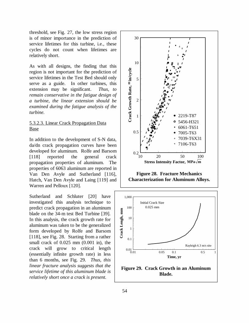
54

threshold, see Fig. 27, the low stress regionis of minor importance in the prediction ofservice lifetimes for this turbine, i.e., thesecycles do not count when lifetimes arerelatively short.

As with all designs, the finding that thisregion is not important for the prediction ofservice lifetimes in the Test Bed should onlyserve as a guide. In other turbines, thisextension may be significant. Thus, toremain conservative in the fatigue design ofa turbine, the linear extension should beexamined during the fatigue analysis of theturbine.

5.3.2.3. Linear Crack Propagation DataBase

In addition to the development of S-N data,da/dn crack propagation curves have beendeveloped for aluminum. Rolfe and Barsom[118] reported the general crackpropagation properties of aluminum. Theproperties of 6063 aluminum are reported inVan Den Avyle and Sutherland [116],Hatch, Van Den Avyle and Laing [119] andWarren and Pelloux [120].

Sutherland and Schluter [20] haveinvestigated this analysis technique topredict crack propagation in an aluminumblade on the 34-m test Bed Turbine [39].In this analysis, the crack growth rate foraluminum was taken to be the generalizedform developed by Rolfe and Barsom[118], see Fig. 28. Starting from a rathersmall crack of 0.025 mm (0.001 in), thecrack will grow to critical length(essentially infinite growth rate) in lessthan 6 months, see Fig. 29. Thus, thislinear fracture analysis suggests that theservice lifetime of this aluminum blade isrelatively short once a crack is present.

10 20 50 1000.2

0.5

1

2

5

30

Stress Intensity Factor,

Cra

ck G

row

th R

ate,

in

/cyc

leµ

2219-T875456-H3216061-T6517005-T637039-T6X317106-T63

MPa m

10

Figure 28. Fracture MechanicsCharacterization for Aluminum Alloys.

0.01 0.05 0.1 0.5 10.01

0.1

1

10

100

1,000

Time, yr

Cra

ck L

engh

, mm

Initial Crack Size0.025 mm

Rayleigh 6.3 m/s site

Figure 29. Crack Growth in an AluminumBlade.

55

Veers and Van Den Avyle [121] have investigated the application of the constant amplitude datato spectral loading conditions. Using the constant amplitude data obtained by Van Den Avyle andSutherland [116], the behavior of 6065-T5 aluminum is characterized using Eq. 39 with theconstants m, p and q set equal to zero. Predictions based on this model are then compared tocrack propagation data obtained under spectral loads. They find that linear models yieldpredictions that are notconservative for this material.

5.3.3. Gears

The AGMA has developed materialproperties and design practices fortypical gear materials [122, 123].A typical S-N diagram used by theAGMA for alloy steels casecarburized to Rockwell C (Rc) 58-63 case hardness and 30-42 corehardness is shown in Fig. 30. Thebreak in the curve, atapproximately 2x106 cycles in Fig.30, is representative of a fatigue orendurance limit. The slope of thecurve after the break is a 34.5 MPa(5 ksi) drop between 2x106 to 108

cycles (see the discussion directlyabove). Additional S-N diagrams for gear materials are available in the literature and directlyfrom gear manufacturers (proprietary data).

5.4. Fiberglass Composites

Composites constructed with fiberglass reinforcements are currently the blade materials of choicefor wind turbine blades. This class of materials is called simply fiberglass composites or fiberreinforced plastics (FRP). In turbine designs, they are usually composed of E-glass in a polyester,vinyl ester or epoxy matrix. Blades are typically produced using hand-layup techniques, butrecent advances in RTM (Resin Transfer Molding) and pultrusion technology have blademanufacturers examining new procedures for increasing the quality of the final product andreducing manufacturing costs.

General references on designing with composite materials are provided in Composites,Engineered Materials Handbook [124] and Tsai and Hahn [125]. Mayer [126] describes the useof fiberglass composites for the design of wind turbine blades.

1E+3 1E+4 1E+5 1E+6 1E+7 1E+8300

500

700

1,000

1,200

1,500

Cycles to Failure

Ben

ding

Str

ess,

MP

a Alloy Steel Case CarburizedGrade 2, L1

Figure 30. S-N Diagram for Carbonized SteelGears.

56

5.4.1. Databases

There are two main fiberglass composite databases for wind turbine applications. The first is theDOE/MSU database that has been developed in the U.S. by Mandell and Samborsky [127], andthe second is the European database. The latter is the compilation of the work of manyresearchers, that has been compiled as the FACT database by de Smet and Bach [128] and therecent compilation by Kensche [16]. The European database is best characterized as the study ofa few materials in great depth, and the former is best characterized as a study of many materials innot as much depth. Here, the DOE/MSU database will be used to illustrate data trends and theEuropean database will be used to bring out the details that are important to the fatigue design ofa wind turbine blade.

5.4.1.1. DOE/MSU

The DOE/MSU database was developed by Mandell et al. in a series of papers [127, 129-137].This database for E-glass composites contains over 4500 data points for 130 material systems. Ahigh frequency database provides a significant data set for unidirectional composites to 108 cycles.Most of the data are presented in terms of maximum initial strain measured in the early stages ofthe test. The database explores such material parameters as reinforcement fabric architecture, fibercontent, matrix materials and loading parameters (R values).

5.4.1.2. European Database

The European database is a compilation of data from many research groups. Most of these datawas collected under the auspices of the European Commission (EC). The objective of the EC’sprogram was to develop the basic information required to set design limits for rotor bladesconstructed with Glass Fiber Reinforced Plastics (GFRP). The compilation of these data is theFACT database [128]. A complete collection of the database, an evaluation of results and adetailed list of the references are provided in Kensche [16]. Only selected references from thisdatabase are discussed here.

5.4.2. Trend Analysis

As discussed by van Delft et al. [138] and used by many other authors, the S-N behavior ofcomposite materials at a constant R value is typically described using either Eq. 34 or 37.Typically, Eq. 37 has been used to characterize the DOE/MSU database [127]. The Europeandatabase is typically fit with Eq. 34, [128, 138].

Equation 37 was chosen to characterize the DOE/MSU database because the fit yields a value forC that is very close to 1. As discussed below, this property is extremely important whencharacterizing composite data, because normalization to the static strength may then be used toeliminate batch-to-batch material variation in the fatigue data.

The formulation shown in Eq. 37 has led to the “ten percent” rule that is typically used as ageneral rule-of-thumb for the tensile fatigue behavior (R ≅ 0.1) of uniaxial composites [139].

57

Namely, the fatigue strength of the composite is reduced by ten percent by each decade of fatiguecycles, i.e., when C is one and b is one tenth (i.e., a fatigue exponent of 10). A similar rule-of-thumb for compressive fatigue behavior (R ≅ 10) reduces the compressive strength byapproximately 7 to 8 percent for each decade, i.e., when C is one and b is 0.07 or 0.08. This formis typically used for composites when comparing different material systems because it normalizesout variations in the static strength. Other typical values for the fatigue exponent m are 3 forwelded steel and 6 for aluminum.

Both forms of the material representation have been used extensively to fit composite fatigue dataand, as discussed later, they have important implications to damage calculations for spectral data.

5.4.3. General Data Trends

A large number of data points from the DOE/MSU database are plotted in Fig. 31. These dataare for fiberglass composites with at least 25 percent fiber in the loading direction tested at R =0.1. When fit with Eq. 37, the good materials have a slope of 0.10 and the poor have a slope of0.14. Thus, the good materials in this figure are approaching the best fatigue behavior that can beobtained for fiberglass materials in tensile fatigue (the ten percent rule for uniaxial composites atR = 0.1) [139], while the poor materials do not perform nearly as well. Indeed, the smallappearing variation in the fatigue slope b produces significant differences in fatigue performance.As shown in the figure, at 20 percent of static strength, the good materials have almost 2.5 ordersof magnitude longer life thanthe poor materials.

Figures 32 and 33 illustrate thetrends for compressive andreverse fatigue. Forcompressive fatigue, the goodmaterials have a slope of 0.07and the poor materials have aslope of 0.11. For reversefatigue, the slopes are 0.12 and0.18, respectively.

Even when a family oflaminates is tested, see Figure34, similar behavior isobserved in tension (R ≅ 0.1),with slopes of 0.10 and 0.14for the good and poormaterials, respectively.8 Thus, 8 In this case, the variation in properties is a direct result of varying the overall volume fraction from 31 percentfor the good material to 54 percent for the poor material. This result is discussed in detail described in section5.4.3.2 “Fiber Content” on p. 60.

1E+0 1E+1 1E+2 1E+3 1E+4 1E+5 1E+6 1E+7 1E+8 1E+90

0.2

0.4

0.6

0.8

1

1.2


Max

imum

Nor

mal

ized

Str

ess,

R = 0.1

IndustialMSU

s s = 1 - b log No

b gσ /σ

o

GOODb = 0.1

POORb = 0.14

Figure 31. Extremes of Normalized S-N Tensile FatigueData for Fiberglass Laminates, R=0.1.

58

a major objective in the development of thisdatabase has been to sort out the differencesbetween the good and the poor materials.

5.4.3.1. Fabric Architecture

The geometry of reinforcing fabrics plays amajor role in static and fatigue properties.Woven glass-fabric composites typically showpoorer tensile fatigue resistance than well-aligned, uniformly dispersed compositesystems [139]. Samborsky et al. [136] give acomparison of static and fatigue properties forseveral types of E-glass fabric laminates with0° plies. Ultimate tensile strength and elasticmodulus are relatively insensitive to fabrictype, but ultimate compressive strength issignificantly lower for fabrics like A130 with aweave geometry that produces an out-of-plane curvature in the strands. Woven fabrics haveabout half the compressive strength of fabrics with straight strands. Mandell and Samborsky [127]note that the compressive fatigue resistance, when normalized by the ultimate compressivestrength, is insensitive to fabric type or fiber content.9

9 The straight-strand fabrics will also have significantly reduced compressive strength if the fibers become “wavy”during fabrication.

1E+0 1E+1 1E+2 1E+3 1E+4 1E+5 1E+6 1E+7 1E+8 1E+90

0.2

0.4

0.6

0.8

1

1.2


Max

imum

Nor

mal

ized

Str

ess,

b = 0.11

σ /σ

o

b = 0.07

R = 10

s s = 1 - b log No

b g

Figure 32. Extremes of Normalized S-NCompressive Fatigue Data for Fiberglass

Laminates, R = 10. Normalized to theUltimate Compressive Strength.

1E+0 1E+1 1E+2 1E+3 1E+4 1E+5 1E+6 1E+7 1E+8 1E+90

0.2

0.4

0.6

0.8

1

1.2


Max

imum

Nor

mal

ized

Str

ess,

b = 0.18

σ /σ

o

b = 0.12

R = -1

s s = 1 - b log No

b g

Figure 33. Extremes of Normalized S-NReverse Fatigue Data for Fiberglass

Laminates, R = -1. Normalized to theUltimate Tensile Strength.

1E+0 1E+1 1E+2 1E+3 1E+4 1E+5 1E+6 1E+7 1E+8 1E+90

0.2

0.4

0.6

0.8

1

1.2


Max

imum

Nor

mal

ized

Str

ess,

b = 0.14

σ /σ

o

b = 0.10

R = 0.1 Materials (Volumn Fraction of Fibers:

DD5 (38%)DD4 (50%) DD7 (54%)

DD6 (31%)DD2 (42%)

s s = 1 - b log No

b g

Figure 34. Extremes of Normalized S-NFatigue Data for a Single Family of

Fiberglass Laminates with 72% 0° Pliesand 28% ±45° Plies, R = 0.1.

59

Typically, the fabrics used inwind turbine applicationhave either stitched or wovenstand structures, see Fig. 35.

A material that wasinvestigated early in thedevelopment of this databasewas a stitched-triax material,i.e., the material contains 0°and ±45° layers that arestitched together withorganic fibers at the factoryto save handling costs duringblade fabrication. Twolaminate constructions withthe same triax fabric werestudied. The first had a 35percent volume fraction offibers and the second had a40 percent volume fraction.Both laminates, calledMaterial AA in the database[127], behaved uniformly inthe poor category, as didmany other types of triaxfabrics [127]. They are veryimportant in this study because they provide an understanding of the basic difference between thebest and worst materials in the entire database.

The essence of the results is that when the stitching is removed, the unstitched-triax behaves asone of the best materials. This observation is also true for an equivalent laminate (same layupschedule) constructed from unstitched 0° and ±45° layers. This result was explained with the aidof a detailed finite element analysis (FEA) of the local fiber stress in the composite near off-axismatrix cracks [129, 131, 135]. As the composite is loaded in tension, the matrix in the off-axis(45°) layers cracks (these cracks start forming at stress levels that are relatively low whencompared to the static strength of the laminate). The FEA analysis of one of these crackedregions demonstrates that a local stress concentration factor of approximately 2.5 is generated inthe 0° strands at the crossing of a 0° and a 45° layer. This large stress concentration is a directresult of the construction techniques used in the triax material. Namely, the organic fibers that areused to tie the various layers of the laminate together hold the glass fibers very close to oneanother, essentially touching. Under normal separation (obtained by not stitching the 0° and ±45°layers together), the stress concentration is approximately 1.4 to 1.7. Thus, the large localstresses produce early failure and uniformly poor fatigue behavior in the stitched triax material.

Figure 35. Dry Fabric Samples.

60

5.4.3.2. Fiber Content

The implication of the previousdiscussion is that behavior ofcomposite systems will, ingeneral, degrade as fiber content,is increased [127]. In earlierwork, Mandell [139] found thatmany woven glass-fabriccomposites show poorer tensilefatigue resistance than the well-aligned, uniformly dispersedsystems. Fig. 36 illustrates thisbehavior in several materials forfiber content, by volume, betweenapproximately 30 and 60 percent.The materials cited in this figureare both cross-plied compositelaminates, [0/±45/0]s, (MaterialsAA and DD) and uniaxiallaminates (Materials A130 andD155). As illustrated in Fig. 36a,material AA (stitched triax plies)has uniformly poor behavior, butwhen the separate, unstitched 0°and ±45° layers are used, there isa transition from good to poorbehavior that begins at anapproximate fiber content of 35percent (see Fig. 34). Note onceagain that the main differencebetween the AA triax and the DDlaminate is that the 0° and ±45°layers in the AA material arestitched together.

Similar data for unidirectionalmaterials are shown in Figure 36b. As shown by data for the A130 (woven), D092 and D155(loosely held together with organic fibers) composites, the optimum fatigue performance isachieved with a fiber content of approximately 40 percent. Moreover, as illustrated by unstitchedD155 material data, if all stitching, be it relatively loose or otherwise, is removed, the progressionfrom good to poor fatigue behavior is delayed to almost 50 percent fiber volume.

25 30 35 40 45 50 55 60 650.08

0.1

0.12

0.14

0.16

Fiber Volume Content, percent

Coe

ffic

ient

, b

AA DD

Figure 36a. Fatigue Sensitivity Coefficient forVarious Fiber Contents in Fiberglass Laminates with0° and ±45° Plies.

25 30 35 40 45 50 55 60 650.08

0.1

0.12

0.14

Fiber Volume Content, percent

Coe

ffic

ient

, b

D092 D155, unstitched

D155A130

Figure 36b. Fatigue Sensitivity Coefficient forUnidirectional Fiberglass Laminates.

Figure 36. Fatigue Sensitivity Coefficient forFiberglass Laminates as a Function of Fiber Content,

at R = 0.1.

61

As discussed above, the origin of the sharp decrease in fatigue resistance as the fiber contentincreases apparently lies in a transition to a condition where the laminate fails in fatigue soon afterthe matrix cracks, usually along the stitching or weave cross-over [127]. When 45° plies arepresent, poor performance is observed if the 0° plies fail soon after the ±45° plies form matrixcracks. Good performance is associated with the 0° fiber wearing-out gradually, as occurs in thetesting of a single strand of material [127, 139].

Thus, the fiber separation is an important parameter for defining the fatigue behavior ofcomposite laminate systems. And, although stitching makes fiber layers and bundles easier tohandle in the manufacturing process, they degrade the fatigue behavior of the composite system.

5.4.3.3. Normalization

The above discussion uses normalized data to enable a relatively large number of laminate systemsto be compared directly to one another. As the static tensile strength is approximatelyproportional to fiber volume fraction, the minimum fatigue coefficient b does not guarantee theoptimum fatigue behavior. Rather, the increased strength offered by more fibers will offset asmall amount of the decrease in the fatigue performance, depending on the design loads for theblade. However, the strain-to-failure in fatigue is much lower (by a factor of approximately 2)for the materials with the poor behavior.

5.4.3.4. Matrix Material

Three matrix materials are commonlyused in the construction of compositeblades for wind turbines. They arevinyl ester, polyester and epoxy. Asreported in the DOE/MSU database[127] and the FACT database [128],the matrix material has minimal effecton the static and fatigue properties ofthis class of composites becausetypical blade materials are primarilyuniaxial. The various resin systemsare compared in Fig. 37. These dataare for tension fatigue (R=0.1) in anunstitched [0/±45/0]s composite.Similar results are obtained in bothcompressive and reverse fatigue.

5.4.4. Modulus Changes

The composite laminates that are typically used in wind turbine blades have very low strain-to-failure in the transverse direction. This characteristic implies that matrix cracking will be presentin the off-axis ±45° plies of a laminated structure long before it fails. As shown in the MSU/DOE

1E+0 1E+1 1E+2 1E+3 1E+4 1E+5 1E+6 1E+7 1E+8200

300

400

500

600

700


Max

imum

Str

ess,

MPa

Material DD5[(0/±45/0)(/0/∓45/0)]36% Fiber Content

EpoxyPolyesterVinylester

R = 0.1

Figure 37. Effect of Matrix Material on TensileFatigue in a Fiberglass Laminate with 0° and

±45° Plies.

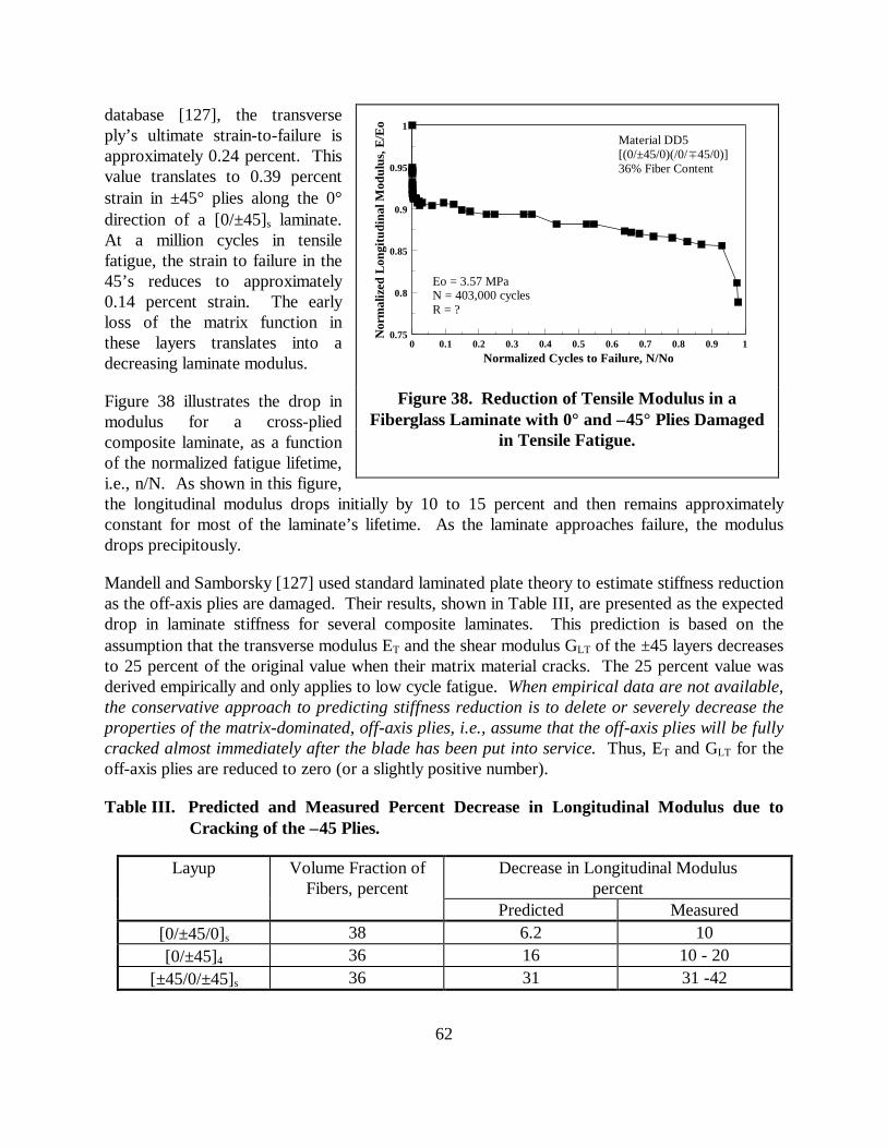
62

database [127], the transverseply’s ultimate strain-to-failure isapproximately 0.24 percent. Thisvalue translates to 0.39 percentstrain in ±45° plies along the 0°direction of a [0/±45]s laminate.At a million cycles in tensilefatigue, the strain to failure in the45’s reduces to approximately0.14 percent strain. The earlyloss of the matrix function inthese layers translates into adecreasing laminate modulus.

Figure 38 illustrates the drop inmodulus for a cross-pliedcomposite laminate, as a functionof the normalized fatigue lifetime,i.e., n/N. As shown in this figure,the longitudinal modulus drops initially by 10 to 15 percent and then remains approximatelyconstant for most of the laminate’s lifetime. As the laminate approaches failure, the modulusdrops precipitously.

Mandell and Samborsky [127] used standard laminated plate theory to estimate stiffness reductionas the off-axis plies are damaged. Their results, shown in Table III, are presented as the expecteddrop in laminate stiffness for several composite laminates. This prediction is based on theassumption that the transverse modulus ET and the shear modulus GLT of the ±45 layers decreasesto 25 percent of the original value when their matrix material cracks. The 25 percent value wasderived empirically and only applies to low cycle fatigue. When empirical data are not available,the conservative approach to predicting stiffness reduction is to delete or severely decrease theproperties of the matrix-dominated, off-axis plies, i.e., assume that the off-axis plies will be fullycracked almost immediately after the blade has been put into service. Thus, ET and GLT for theoff-axis plies are reduced to zero (or a slightly positive number).

Table III. Predicted and Measured Percent Decrease in Longitudinal Modulus due toCracking of the ±45 Plies.

Layup Volume Fraction ofFibers, percent

Decrease in Longitudinal Moduluspercent

Predicted Measured[0/±45/0]s 38 6.2 10[0/±45]4 36 16 10 - 20

[±45/0/±45]s 36 31 31 -42

0 0.1 0.2 0.3 0.4 0.5 0.6 0.7 0.8 0.9 10.75

0.8

0.85

0.9

0.95

1

Normalized Cycles to Failure, N/No

Nor

mal

ized

Lon

gitu

dina

l Mod

ulus

, E/E

o

Eo = 3.57 MPaN = 403,000 cyclesR = ?

Material DD5[(0/±45/0)(/0/∓45/0)]36% Fiber Content

Figure 38. Reduction of Tensile Modulus in aFiberglass Laminate with 0° and ±45° Plies Damaged

in Tensile Fatigue.

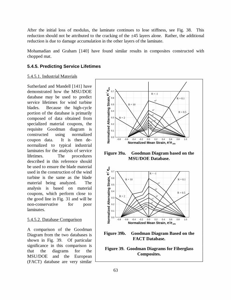
63

After the initial loss of modulus, the laminate continues to lose stiffness, see Fig. 38. Thisreduction should not be attributed to the cracking of the ±45 layers alone. Rather, the additionalreduction is due to damage accumulation in the other layers of the laminate.

Mohamadian and Graham [140] have found similar results in composites constructed withchopped mat.

5.4.5. Predicting Service Lifetimes

5.4.5.1. Industrial Materials

Sutherland and Mandell [141] havedemonstrated how the MSU/DOEdatabase may be used to predictservice lifetimes for wind turbineblades. Because the high-cycleportion of the database is primarilycomposed of data obtained fromspecialized material coupons, therequisite Goodman diagram isconstructed using normalizedcoupon data. It is then de-normalized to typical industriallaminates for the analysis of servicelifetimes. The proceduresdescribed in this reference shouldbe used to ensure the blade materialused in the construction of the windturbine is the same as the bladematerial being analyzed. Theanalysis is based on materialcoupons, which perform close tothe good line in Fig. 31 and will benon-conservative for poorlaminates.

5.4.5.2. Database Comparison

A comparison of the GoodmanDiagram from the two databases isshown in Fig. 39. Of particularsignificance in this comparison isthat the diagrams for theMSU/DOE and the European(FACT) database are very similar

-0.8 -0.6 -0.4 -0.2 0.0 0.2 0.4 0.6 0.8 1.00.0

0.1

0.2

0.3

0.4

0.5

0.6

0.7

Normalized Mean Strain, Nor

mal

ized

Alte

rnat

ing

Str

ain,

uts

ε/ε

010

R = 0.5

R = 0.1

R = -1

R = 10

102

103

104

107

108

R = 2105

106

utsε/ε

Figure 39a. Goodman Diagram based on theMSU/DOE Database.

uts

ε/ε

-0.8 -0.6 -0.4 -0.2 0.0 0.2 0.4 0.6 0.8 1.00.0

0.1

0.2

0.3

0.4

0.5

0.6

0.7

Normalized Mean Strain, Nor

mal

ized

Alte

rnat

ing

Str

ain,

R = 0.5

R = 0.1

R = -1

R = 10102

103

104

107

108

R = 2105

106

utsε/ε

Figure 39b. Goodman Diagram Based on theFACT Database.

Figure 39. Goodman Diagrams for FiberglassComposites.

64

to one another on the tension side (right side) of the diagram and very dissimilar to one anotheron the compression side (left side). This variation is a significant change in the form of theGoodman diagram. In particular, the MSU/DOE database yields a highly non-symmetric diagramwith a strain to failure of 2.7 and 1.5 percent for tensile and compressive strengths, respectively[132]. This ratio of the tensile and compressive failure strains of 1.80 is significantly differentfrom the European database which has a ratio of 1.33. Namely, the European database yields anapproximately symmetric (about the zero mean-stress axis) Goodman diagram with strain-to-failure of 2.58 and 1.94 in tension and compression, respectively [128]. A symmetric diagramimplies that there are only small differences between tensile and compressive failures.

Although they could not prove it, Sutherland and Mandell [141] suggest that the discrepancy inthe compressive failure-strain reflects the difference in compressive testing techniques. Inparticular, the compressive tests conducted for the MSU/DOE database used gauge sections withno lateral supports, whereas, the FACT database has a preponderance of data obtained fromcompression tests with lateral constraints. A sample of the more recent data from the MSU/DOEdatabase illustrates that the ratio of the ultimate tensile to the ultimate compressive strain variesfrom 0.94 to 2.23 with an average value of 1.50 [127]. Thus, differences in the databases can beattributed entirely to material variation. However, the differences in the testing techniques shouldnot be discounted. Detailed comparisons of fatigue data from identical materials will be requiredto sort out the differences in the two databases.

When the two databases are compared on a non-normalized basis, the FACT data are found tocontain a preponderance of the data that behave as the good material in the MSU database. Thus,the MSU/DOE database will predict a service lifetime that is equal to or shorter than thatpredicted by the FACT database.

Sutherland and Mandell [141] investigated the effect of these differences on predicted servicelifetimes. Using the WISPER-protocol U.S. wind farm load spectrum (see the discussion insection 4.8.1.2 “U.S. Wind Farm Spectrum” on p. 38), the predicted service lifetimes for tensilefailure were comparable (44.9 to 67.5 years based on the MSU/DOE and the FACT databases,respectively). However, for compressive failures, the predictions differed by approximately afactor of 5 (23.5 and 136 years, respectively).

5.4.6. Spectral Loading

As discussed extensively above, wind turbines are subjected to spectral loads that are unique tothis structure. Test spectra have been proposed, and fatigue data on material behavior are beingobtained. However, to date, these data are limited in extent. Van Delft et al. [138, 142, 143]have examined the differences between the response in fiberglass to constant and variableamplitude loading using the WISPER and the WISPERX spectrum. Their experiments on apolyester fiberglass laminated with 0° and ±45° layers at approximately 32 percent fiber volumeprovide insight into using constant amplitude S-N data to predict service lifetimes under thespectral loads normally encountered by wind turbines.

65

5.4.6.1. WISPER vs. WISPERX

As discussed in section 4.8.1.1“WISPER” on p. 37, theWISPERX load spectrum is theWISPER spectrum with the smallcycles removed. Damage estimatespredict that the removal of thesmall cycles should have less than a10 percent effect. However, themeasured data indicated that adifference of the order of 50percent (a factor of 2) is actuallyobserved, see Fig. 40. These dataimply that the low-amplitude cyclesare more damaging than suggestedby the constant amplitude S-Ndata.

Also the fatigue exponent b is changed from approximately 0.10 for the constant amplitude datato approximately 0.12 for the spectral data, a significant change.10

5.4.6.2. Predicted Service Lifetime

Van Delft et al. [138, 143] have used the constant-amplitude European database to predict theresponse of composite coupons to the WISPER and the WISPERX loads. Lifetimes werepredicted using Miner’s rule and a power-law fit, see Eq. 32, to constant-amplitude S-N data foran R-value of a -1 (reverse loading). The data were expanded to a full Goodman diagram using aGoodman rule of the form shown in Eq. 38. The predicted service lifetime is approximately twoorders of magnitude higher than the measured lifetime. However, when the S-N data were fit toa log-linear curve, Eq. 35, the predicted and measured service lifetimes were essentially the same,with the predicted service lifetime being slightly conservative.

In another study, Echtermeyer et al. [144] compared the predicted and measured fatigue life forseveral composite laminates to WISPERX spectral loads. These predictions of service lifetimeswere based on a Goodman diagram constructed from S-N data for R-values of 0.1, -1 and 10.These data were fit best using a log-log representation. In one laminate, the predictions agreedwith measured lifetimes. In two others, the prediction was a factor of approximately 5 higherthan the measured lifetime. And in the final laminate, the predictions varied between a factor of 4higher to a factor of 0.6 lower.

10 In this case, the exponent being compared is based on the fit of the S-N curve for the number of the WISPER orWISPERX load sequences to failure.

1 3 10 30 100 300 1000100

200

300

400

Number of Sequences

Max

imum

Str

ess,

MPa

b = 0.120

b = 0.122

WISPER

WISPERX

σ σ = 1 + b log No b g

Figure 40. S-N Diagram for a Fiberglass Laminatewith 0° and ±45° Plies, under WISPER Loading

Conditions.

66

Thus, the behavior of composites under typical wind turbine loads is not well understood and isthe subject of on-going research in various wind programs throughout the world. Based on thelimited data discussed above and the data presented in Fig. 40, we can surmise that the lowamplitude fatigue cycles are more damaging than indicated by the constant-amplitude S-N data.

5.4.7. Structural Details

The extension of coupon data to the behavior of full-size structural components is being studiedby Mandell et al. [127, 134, 145-148]. The results of their studies on such details as ply drops,local fiber content and transverse cracks are summarized in Table IV. The “knock-down” factorF in this table is defined to be the ratio of the maximum cyclic strain (R = 0.1) of a uniformcoupon to that of a structured coupon at one million (106) cycles; namely:

F = Uniform Coupon Strain @ 10 Cycles

Structured Coupon Strain @ 10 Cycles

6

6 . (45)

5.4.7.1. Ply Drops

One common feature of blade structures is the use of ply drops to tailor the thickness of thecomposite structure to meet loads criteria while minimizing weight. In the detailed studies byCairns et al. [134, 146], several configurations for the ply drops have been experimentallyinvestigated and analyzed. As shown in Fig. 41, the ply drop may be internal (covered by at leastone layer of fabric) or external.

The internal ply drop creates local stress concentrations that initiate failures. As shown in TableIV, these local stress concentrations cansignificantly reduce fatigue lifetimes.The investigation illustrated thatinternal ply drops are less susceptibleto delamination than external ply dropsand that for the same ply drops, thickerlaminates are better in resistingdelaminations. As indicated by anincreased knockdown factor [127],dropping two plys in the same locationis twice as harmful as dropping a singleply, and that feathering (i.e., staggeringadjacent tows) or “Z-spiking11“ the plywill significantly decrease delaminationgrowth rate.

11 Z-spiking consists of plunging some of the fibers from the ply drop edge into the adjacent layers (the z-direction).

Figure 41a. External Ply Drop.

Resin Rich Area

Figure 41b. Internal Ply Drop.

Figure 41. Typical Ply Drop Configurations.

67

Table IV. Knock-Down Factors for Selected Structural Details in Tension andCompression for Approximately 70% 0° Materials.

DETAIL SKETCH KNOCK-DOWN FACTOR, F

A 130Fabric

D155Fabric

UC1018VFabric

Simple Coupon(Straight Material)

1.0 1.0 1.0

Surface IndentationTension, R=0.1

(Vf increased, thickness reduced by25%)

r = 6 mmV = 45-52 %f

V = 35-37 %f 1.6 2.5 1.2

Surface IndentationCompression, R=10

(Vf increased, thickness reduced by25%)

r = 6 mm

V = 52 %f

V = 37 %f 1.0 1.4 --

Locally Higher Fiber ContentTension, R=0.1

(2-90° Piles in center)

V = 34 %f

V = 47 %f

2.1 1.5 --

Locally Higher Fiber ContentCompression, R=10

(2-90° Piles in center)

V = 34 %f

V = 47 %f

1.0 1.4 --

Exterior Cracked TransverseTension, R=0.1

90° Patch

-- 1.0 --

Double Interior 0° Ply DropTension, R=0.1

V 40 %f <

1.4 1.6 --

68

5.4.7.2. Locally Higher Fiber Content

As discussed above (see the discussion in section 5.4.3.2 “Fiber Content” on p. 60), the fiberglasslaminates typically used in wind turbine blades are susceptible to significant degradation in theirfatigue properties if fibers are forced very close to one another. The effect is noted in thedependence in fatigue coefficient on fiber density shown in Fig. 36. This effect also translatesinto local manufacturing defects, simulated by surface indentations and excess fiber layers. Asshown in Table IV, a surface indentation produces a knock-down factor of 2.5 for a local increasein fiber content from 35 percent to 47 percent in tension. In compression, the knock-down factoris 1.4 for a local increase in the fiber volume from 37 percent to 52 percent.

5.4.7.3. Transverse Cracks

In typical lay-ups of composite structures and especially for wind turbine blades, a high percent ofthe fibers is aligned with the primary load direction. Additional off-axis layers are added toprevent splitting and to increase shear properties. As discussed above, these off-axis layers aretypically more susceptible to fatigue damage. Ideally, these layers would split off from theunderlying layers that carry the main loads without causing them to fail prematurely.12 Thus,Table IV supports the concept that no knock-down factor is required for the propagation oftransverse cracks into uniaxial composites. As discussed above, this factor is based on theassumption that fiber separation is adequate to prevent the fiber density effects discussed above.

5.4.7.4. Environmental Effects

As discussed by Kensche [16], wind turbine blades are subjected to a hostile environmentthroughout their service lifetimes. The primary effects include ultra violet (UV) radiation;temperature fluctuations; rain, ice, humidity; thunderstorms/lighting; hailstones; erosion from sandparticles; and extreme dryness in desert environments. A matrix-rich outer-layer of gel coat istypically applied to the blades to provide UV protection and to seal the exterior surface of thecomposite.

Kensche [16] summarizes the degradation of the mechanical properties of various laminatesystems used in wind turbine blades and presents a general discussion of the topic. Bach [149]presents a general discussion of the influence of moisture on bolted joints in composite materials.

In terms of fatigue behavior for composite laminates in turbine applications, the three mostimportant environmental factors are attacks on the matrix material by temperature, humidity andUV radiation. The gel coating offers good protection from UV radiation. Temperature alone istypically not an important environmental parameter because the turbine blades are designed for aspecific range of operating temperatures and the laminate’s matrix is chosen to meet those

12 Thus, the resulting failure of the cross section will be a relatively slow event that can be detected beforecatastrophic failure of the section (and the blade) occurs.

69

conditions.13 However, temperature and humidity combined to become the primaryenvironmental factors that must be considered in the fatigue design of the blade. The discussionshere will concentrate on these two environmental factors.

5.4.7.5. Equilibrium Moisture Content

Under time-varying environmental loads, Fick’s law [16] may be used to predict moisture content.Several authors have used this technique to analyze the yearly cycle of environmental loads oftemperature, humidity and rain on a turbine blade. Kensche [16] used this technique to analyzethe moisture content of a blade subjected to a yearly cycle of cold-wet and warm-dry conditions.His predictions indicate that the moisture content will stabilize at 0.4 to 0.5 percent. Similarsimulations have been conducted by de Bruijn [150, 151] for the Dutch climatological cycle; seethe discussion in section 5.4.7.8 “EN-WISPER Spectrum” on p. 70. For this set of conditions,the total moisture content is predicted to stabilize at approximately 0.25 percent. Measurementsfrom a blade exposed to the Dutch environment for approximately four years agrees with the 0.25percent prediction.

A question does arise concerning the use of the Dutch (northern European) climatological cyclefor a general characterization of the behavior of composites under environmental loads. TheDutch cycle, and for that matter, a typical U.S. climatological cycle, is relatively benign. Turbinesdesigned for deployment in other regions, e.g. India, will have significantly higher environmentalloads. Designers of advanced composite structures (e.g., those using carbon fibers) considerVietnam’s climatological cycle as their extreme case. Thus, a moisture content of of 0.4 to 0.5percent is non-conservative for many applications.

5.4.7.6. Matrix Degradation

The matrix materials used in turbine blades are typically polymeric materials that absorb moisturefrom the humidity in the surrounding air and/or from water lying on their surfaces. Thetemperature governs the velocity of the diffusion process, and the humidity governs the moisturecontent. As the moisture content increases, the glass transition temperature, Tg, of the matrix isdepressed, and the matrix will swell. Eventually, microcracks (crazing) may form in the matrix.Depending on the physical and chemical properties of the matrix (i.e., toughness, etc.), thesechanges may destroy the structural integrity of the laminate. This damage to the matrix hasminimal effect on the tensile behavior of the laminate because the fibers are the primary loadcarrier. However, these effects are significant in compression and shear, where the matrix is theprimary load carrier.

13 Differential thermal expansion can damage components of the wind turbine blade. However, as thermalexpansion is more of a structural design problem than a material problem, it is not considered here.

70

5.4.7.7. Property Degradation

Kensche [16] presents a detailed examination of the effects of absorbed moisture on the physicalproperties of a typical epoxy laminate system. In this set of data, the test specimens have beenpreconditioned using continuous hot-wet conditions. These conditions are 90 percent humidity at45°C. Under these conditions, specimens reach equilibrium in approximately 120 days withmoisture content between 0.4 and 0.5 percent.

When comparing the properties of moist and dry virgin specimens, the static tensile strength wasessentially not affected by absorbed moisture (as one would anticipate). The static compressivestrength was reduced by approximately one third and the interlaminar shear strength by slightlyover ten percent.

Figure 42 compares the fatigueperformance of wet and dry samplesunder reverse loading (R = -1). Thesedata illustrate that the strain-to-failure fora given lifetime (number of cycles tofailure) is reduced by 15 to 20 percent.With the larger value occurring in thelow-cycle region.

Mandell [152] predicts similar results incompression tests of fiberglass couponssubjected to distilled water at 40°C forapproximately 190 days. Under theseconditions, the polyester matrix has aweight gain of approximately 3 percent.The compressive strength of thesecoupons is reduced by 10 to 20 percentwhen tested at room temperature. Whentested at 50°C, the compressive strengthis reduced by 20 to 35 percent.

5.4.7.8. EN-WISPER Spectrum

As discussed above, many of these tests are based on pre-conditioning the samples in a hot-wetenvironment. However, wind turbine blades in the field undergo a series of environmentalchanges, typically on an annual cycle that both adds and removes absorbed moisture from theblade. To help quantify the effects of field environment, de Bruijn [150, 151] and Joosse [153]have proposed a reference environmental spectrum. The spectrum is based on the annual Dutchclimatological cycle, summarized and idealized (simplified) in Table V. The accelerated pre-conditioning cycle they proposed to simulate this climatological cycle is shown in Table VI. Bothsimulations and field measurements were used to validate that the accelerated cycle reproducedboth the moisture profile and the moisture content.

ε /ε o

1E+0 1E+1 1E+2 1E+3 1E+4 1E+5 1E+6 1E+7 1E+8 1E+90

0.2

0.4

0.6

0.8

1

1.2


Max

imum

Nor

mal

ized

Str

ain,

Dry

Wet

Run Out

R = -1

Figure 42. S-N Diagram for a FiberglassLaminate with 0° and ±45° Plies, under Wet

and Dry Environment Conditions.

71

Table V. Idealized Annual Climatological Cycle for the Dutch Environment.

Condition Time, days T, °C ∆T,°C/hour

Relative Humidity,percent

Normal 228 10 5* 80

Hot 5.5 32 -5* 50

Frosty 22 -15 5* 85

Wet 109 8 100 *Rate of change of the temperature from the current to the next condition.

Table VI. Accelerated Climatological Cycle for the Dutch Environment.

Condition Time, days T, °C ∆T,°C/hour

Relative Humidity,percent

Normal 105 18 50* 85

Hot 2.5 45 -50* 40

Frosty 10 -23 50* 100

Wet 49 16 100 *Rate of change of the temperature from the current to the next condition.

When tested, the S-N data from samples that have been pre-conditioned by the EN-WISPERspectrum are not significantly different from non-conditioned specimens; in contrast with thehot-wet pre-conditioned specimens discussion above. Joose [153] attributes this apparentdiscrepancy to a dominance of the test on the ambient conditions during the test. Implications ofthis observation are many. However, as noted by Joose, some test procedures have been calledinto question and require more study. Thus, the pre-conditioned hot-wet samples do bound theproblem, but the penalties in material performance they predict are probably too high for actualfield conditions in Northern Europe and in most of the U.S. This may not be the case for Indiaand Southeast Asia.

5.4.7.9. Effects of the Environment

At this time, environmental effects on composite turbine blades are not well understood, and arecurrently a subject of research, discussion and speculation. For instance, some studies ofadvanced composites for aircraft indicate that the daily maximum use temperature is moreimportant than the average temperature. Thus, current databases may yield non-conservativedesigns for environmental loads. And, the designer should use them only with extreme care.

5.4.8. Comments

The design of composite materials for wind turbine blades has relied heavily on fiberglasstechnology. This material system has proven adequate to the task, even though it must withstand

72

extremely large numbers of fatigue loads with varying amplitudes under extreme environmentalconditions. Potential areas for increasing the performance of this system have been identified andare being pursued. In addition to increasing the performance characteristics of the materialssystem, an understanding of the influence of spectral and bi-axial loading on cumulative damagerules must be developed [154]. Also, design criteria for full-sized structures that are based oncoupon data must be determined.

As blades become larger, stiffness considerations are becoming more and more important to thedesign. Fiberglass systems may not be able to meet these requirements within reasonable designconstraints on weight. The obvious answer to this design issue is to introduce stiffer fibers, i.e.,carbon fibers, into the composite system. Typically, carbon fiber designs have been too expensivefor wind turbine applications. However, mixed fiber designs are currently under considerationand appear to be cost effective. These systems are not represented in the databases describedabove, but will need to be added. Specifically, the composite system with a mix of glass andcarbon fibers will have to be addressed.

5.5. Fatigue Limit Design

The use of a fatigue limit for the fatigue analysis of structures is based on the observation thatsome metals have an essentially infinite life when tested at or below the value of their fatigue limit.Thus, the structural design is based on reducing the stress level at the highest load to the fatiguelimit.

In terms of the S-N curve, an infinite life translates to a zero slope. Most materials do not have atrue fatigue limit. However, many metals exhibit a significant reduction in the slope of their S-Ncurve as the number of cycles to failure gets very large. Figures 27 and 30 illustrate this behaviorin aluminum and steel, respectively. For this class of behavior, a fatigue limit analysis can beconducted by assuming a quasi-fatigue limit that corresponds to the largest number of the cyclesthe structure will have to bear. In Fig. 27, the quasi-fatigue limit would be between 60 and 80MPa for 109 cycles; in Fig. 30 the limit occurs at approximately 2x106 cycles.

The existence of a true or quasi fatigue limit is usually based on the experimental data obtainedfrom constant amplitude fatigue tests. In many cases, when these materials are tested withvariable amplitude loads, the initial slope of the S-N curve does not change as the number ofcycles become very large, see section 5.3.2.1 “S-N Data Base” on p. 52. Because wind turbinesare subjected to spectral loads, the use of constant-amplitude fatigue limit is probably notappropriate for most materials used in wind turbine structures.

5.6. Partial Safety Factors

The IEC has adopted a set of partial safety factors in IEC-61400-1[17] to account for theuncertainties and variabilities in material properties (and in loads). For material properties, thepartial safety factors are included for the following: unfavorable deviations of the strength ofmaterial from the characteristic value; inaccurate assessment of the resistance of sections or load-carrying capacity of parts of the structure; uncertainties in the geometrical parameters; and

73

uncertainties in the relation between the material properties in the structure and those measuredby tests on control specimens. A discussion of partial safety factors and their application to windturbine design is beyond the scope of this report and is not discussed here.

75

6. INFLOW

6.1. Annual Average Wind Speed

The determination of damage in a wind turbine is predicated on the development of a loadspectrum for the turbine. As shown in Eq. 11, the typical formulation uses the annual averageprobability density function for the wind speed as a primary parameter in the description of theload spectrum. Rohatgi and Nelson [155] provide a detailed discussion of annual wind speeddistributions and they provide a compilation of the annual average wind speed for numerous sites.

6.1.1. Formulation

The annual wind speed distribution is typically posed as a probability density function [155]. TheWeibull distribution that is discussed in Appendix A has proven to be particularly effective indepicting the annual wind speed distribution above approximately 3 m/s at a number of U.S. andworld sites [4]. This two-parameter distribution takes the following form:

p = U

exp -U

Uαβ β β

α αLNM

OQPLNM

OQP

LNM

OQP

RS|T|UV|W|

− 1

, α β > 0, > 0, > 0Ub g , (46)

where pU is the probability density function, α and β are the shape factor and the amplitude factorof the distribution, respectively. As cited in Eq. A-3, the average annual wind speed, U , is givenin terms of the Weibull parameters by:

U = 1 + 1βα

Γ LNM

OQP , (47)

where Γ[•] is the gamma function.

6.1.2. Typical Distributions

Extensive data have been gathered,collated and published that describe theannual wind speeds for the U.S. andvast regions of the world [3, 155, 156and 157]. Typical annual wind speeddistributions for several characteristicmembers of the Weibull distributionfamily are shown in Fig. 43. For thisexample, β is normalized to a value ofone.

Because the measurement and analysis

α = 2.8β = 1.0

1.61.2

1.0 − Exponential Distribution

2.4

2.0 − Rayleigh Distribution

0 0.5 1 1.5 20

0.5

1

Normalized Wind Speed

Prob

abili

ty D

ensi

ty F

unct

ion

Figure 43. Weibull Probability DensityFunctions for Various Shape Factors.

76

of these data are outside the scope of this report and they appear elsewhere in the open literature,detailed discussions of this subject are not presented here.

6.2. Inflow Characteristics

While “… tempting to think of wind as a constant homogeneous velocity field of fixed direction,”the inflow is actually a three-dimensional, inhomogeneous, and unsteady flow field [4]. Thechallenge to the modeler is to describe those characteristics of the inflow that produce loads onthe turbine. The three principal characteristics that have found favor with designers are the meanhorizontal wind speed, the turbulence and the vertical shear.14 As discussed above, this parameterset is probably not sufficient. Moreover, at this time, there is no clear picture as to which inflowparameters govern the loads on the various machine configurations. This section describes someof the atmospheric/inflow parameters that are currently being studied as potential predictors ofturbine loads through the characterization of the inflow.

6.2.1.1. Turbulence

The primary characterization of the instantaneous flow field into the rotor has been the single-point turbulence intensity measured at hub-height in front of the turbine [5]. If the instantaneoushorizontal velocity at rotor height, denoted by u(t), is separated into its long-term component Uand its fluctuating value (about zero mean), such that,

u t = u t + Ub g b g¢ , where (48)

U = 1T

u t dt0

T b gz . (49)

As noted above, the averaging time T is typically 10 minutes. The turbulence intensity Iu is theRMS of u' divided by its long-term average U. Namely,

I = uU

= 1U

1T

u dtu2

0

T$ ¢LNM

OQPz b g

12

. (50)

The parameter $u is commonly called the turbulence.

When determining operational loads on a turbine, each mean wind speed bin is assumed to have aweighted summation of the loads across the expected distribution for turbulence intensity.

14 Variations in the inflow velocity can be separated into mean and turbulent components (i.e., long-termvariations can be separated from short-term variations) because the power spectrum of the velocity of the inflow isdivided naturally into two peaks. The low-frequency peak defines the variation of the mean inflow velocity and thehigh-frequency peak defines the turbulence. The peaks are separated by a spectral gap that covers the range fromapproximately 5 minutes to 2 hours [5].

77

6.2.1.2. Vertical Shear

The wind shear exponent α is typically used to characterize the variation of the mean wind speedfrom the bottom of the rotor disk to its top. In this form, the wind speed U as a function of heightis given by:

U zU z

= zz

1

2

1

2

b gb g

LNM

OQP

a

, (51)

where z is the height above the prevailing terrain.

Wind shear is an integral part of the certification standard for wind turbines, and must be includedin all structural analyses.

6.2.1.3. Additional Inflow Parameters

While turbulence and vertical shear are the two parameters typically used to describe the inflow,many additional inflow parameters are being investigated as descriptors for the inflow, or thereby,as predictors of turbine loads. In one of the more comprehensive experimental examinations ofthe relationship between inflow and fatigue loads to date, Mouzakis et al. [158-161] examine along list of inflow statistics to determine which are important for introducing fatigue loads into theturbine. Their list includes mean horizontal velocity, standard deviation of the inflow in threedirections, wind shear exponent, the skewness and kurtosis of the inflow in the primary flowdirection, turbulence length scales in three directions and the Davenport decay factors for timeand space between the hub and the top of the rotor. The turbulence length scale is a measure ofthe average size of eddies in the inflow [5]. The longitudinal length scale xLu is defined in terms ofthe cross-correlation function R(r) by the following:

xu 0

L = R r drb g•z , (52)

where

R r = 1T

u x, t u x + r, t

udt2

to - T2

to + T 2 b g b g b g∑z $ . (53)

Using a regression analysis on three wind-speed bins that cover 7-9, 12-14, and 16-18 m/s,Mouzakis et al. calculate the correlation coefficient between fatigue loads and inflow statistics.Their evaluation of blade loads in mountainous terrain illustrates that the standard deviation ofthe vertical component of the inflow, $w , dominates the flatwise blade loads. This parameter wasfollowed in importance by the average inflow velocity U, the standard deviations of the horizontalwind speed components (parallel and perpendicular to the direction of the average wind speed)and the wind shear exponent α. Some additional dependencies were noted for the skewness andkurtosis of the inflow. For edgewise blade loads, the inflow velocity U was the primary

78

parameter, with standard deviations of the vertical and horizontal wind speed components, andthe shear exponent α following in their order of importance.

6.2.1.4. Reynolds Stresses

Kelley [49, 50] and Kelley and McKenna [51] have examined several other parameters fordescribing the inflow. The first are the Reynolds stresses. In a 3D flow field, these stresses arethe average cross products of the fluctuating components of the inflow,

¢¢ ¢¢ ¢¢u w , u v and v wb g b g b g , (54)

where u' and v' are the fluctuating components of the wind speed in the horizontal directionparallel and perpendicular to the direction of the average wind speed, respectively, and w' is thevertical component.

Richardson Number: Continuing the evaluation, Kelley et al. [49, 51] examined the gradientRichardson number, Ri. This parameter is a measure of the atmospheric stability between twoelevations. For wind turbine applications, the two elevations are typically chosen with thereference elevation relatively close to ground level, denoted here with the subscript 1, and theother, the subscript 2, at the top of the rotor disk. If T is the temperature in degrees centigradeand the atmospheric pressure in hPa, then the layer mean potential temperature is given by:

Q i ii

= T + 273.16 1000

Pb g L

NMOQP

0 286.

. (55)

The over bar on a quantity denotes its 10-minute average. The index i refers to the verticalposition z of the measurement, i.e.; i = 1 refers to the reference height (typically near groundlevel) and i = 2 refers to an elevated height. Then the Ri is given by:

Ri = 2 g +

- z - z

U - Uz - z

1 2

2 1

2 1

2 1

2 1

Q Q

Q QFHG

IKJ L

NMM

OQPP

d ib g

d ib g

2 , (56)

where g is the gravitational acceleration (m/s2). Based on the Richardson number, the atmosphereis said to be unstable when Ri < 0, near-stable when 0 ≤ Ri < 0.01 and stable when Ri ≥ 0.01.

Obukhov Length Scale: The final parameter investigated by Kelley et al. [49, 51] is the Obukhovlength scale. This length is measured at a single elevation. This parameter is used in boundarylayer turbulence scaling and is related to the gradient Richardson number. When divided into theelevation of the measurement, the result is the Monin-Obukhov stability parameter. In unstable

79

flows, the Richardson number is identical to the Monin-Obukhov stability parameter [49]. TheObukhov length scale is given by:

L = - u' w'

0.4 g w' '

qq

b gb g

32

, (57)

where ¢¢u wb g is the time average of the cross product of the fluctuating velocity components u'

and w' described in Eq. 54 and w' 'qb g is the time average of the product of w' and the

temperature θ' is fluctuating temperature components about the average temperature q .

Kelley found that the flap bending loads were dominated by the vertical component of the

Reynolds stress ¢¢u wb g . Thus, this term and the Richardson number dominate the edgewise-bending loads.

6.2.1.5. Summary

The effects of many inflow parameters have been shown to significantly influence turbine loads.Current practices reduce inflow descriptions to the mean horizontal inflow velocity, wind shearand the turbulence intensity. However, additional parameters must be examined to ensure that acomplete set of loads on an operating turbine has been obtained; see section 4.4.2 “InflowParameters” on p. 26.

81

7. SOLUTION TECHNIQUES

The solution of Eq. 11,

1T

= p n , , U

N , d d dU = t U

U

Um a

m a0-a m

in

out

∆D z zz ∞

∞

∞ σ σσ σ

σ σb gb g , (11)

for the damage rate in a wind turbine component can take many forms, depending on theassumptions about its characteristics. In this section of the paper, various solution techniques arepresented.

7.1. Closed Form Solution

Although most solutions to Eq. 11 are numerical in form, Veers et al. [162, 163] have posed aclosed form solution. The groundwork for this solution was laid by Veers in his analyses of theservice lifetimes for VAWTs [18, 43-45]. As with all solutions, and in particular with closed formsolutions, the assumptions behind the solution are very important.

7.1.1. Basic Assumptions

7.1.1.1. Annual Wind Speed Distribution

The wind speed distribution is assumed to be a Weibull distribution of the form cited in AppendixA and shown in Eq. 46. This two-parameter distribution is a function of the average annual windspeed U and the shape factor αU.

7.1.1.2. Cyclic Stress

The distribution of cyclic stresses is also assumed to have a generalized Weibull distribution of theform shown in Eq. 24. The standard deviation of the cyclic stresses is assumed to depend directlyon the mean wind speed. In this case, the dependence takes the form of a power law, namely:

σ σ = K U

Ucharchar

pFHG

IKJ , (58)

where K is the stress concentration factor that relates global stresses to local stresses, and σchar isthe standard deviation of the cycle count distribution at a wind speed of Uchar. The Weibullparameter for this distribution is αs. The stress cycles are all assumed to have the same mean σm;see the discussion in section 4.5.4 “Mean Value Bins” on p. 30.

The rate at which these cycles are occurring is assumed to be a power series in wind speed of theform:

82

F f f f= + FHG

IKJ+ F

HGIKJ0 1 2

2U

UU

Uchar char

. (59)

7.1.1.3. Material Behavior

The S-N curve is taken to be a straight-line fit on a log-log scale of the form cited in Eq. 31.Veers et al. have chosen to write the equation as follows:

N CK

( )s s sss

a ma

m

u

b

,

=-

F

H

GGGG

I

K

JJJJ

-

1 , (60)

where the Goodman correction, see Eq. 38, based on the ultimate stress σu is used to include theeffect of the constant mean stress σm.

7.1.1.4. Damage Rule

Miners Rule assumes that failure occurs when the damage equals one; i.e., when the damage rate∆Dt in Eq. 11 for a representative time t multiplied by the projected lifetime T equals 1, see Eq. 6.However, depending on the material and the load spectrum, failure can occur at values of D thatvary widely from one. For this analysis, failure is assumed to occur at a value of δ.

7.1.1.5. Run Time

The turbine is assumed to be available for the fraction A of each year of its operational lifetime,and the turbine is assumed to operate in all wind speeds between 0 and the cut-out wind speedVout.

7.1.2. Solution

For the case, V out Æ • and F = fo, the predicted service lifetime T equals

TC

A 1 K /U

Ub bpchar

m u char U

bp

s U

=FHG

IKJ −

FHG

IKJFHG

IKJ

FHG

IKJFHG

IKJ

RS|T|

UV|W|

−

da

ss s a a af

K

s

b b

0

2 1

22 1/ ! / !

! !/

b g b g , (61)

where the factorial (•)! is the gamma function.

The solution of this equation can be computed directly or by using the FAROW computer code[163].

83

7.2. Numerical Solutions

7.2.1. The LIFE Duo of Fatigue Analysis Codes

The initial analysis of the load spectra on a VAWT was addressed by Veers [18, 43-45]. Theseanalyses laid the foundation for the LIFE series of fatigue analysis codes [164]. This formulationis essentially the numerical solution of Eq. 61 with a more restrictive set of assumptions; namely,the narrow-band Gaussian model for the stress spectra with a constant mean stress and cyclicfrequency, a Rayleigh wind speed distribution, and a log-log description of the S-N curve. Theinitial code was later modified and used by Akins [165] and Malcolm [166]. Sutherland et al.[167] released the final version.

The great strength of the LIFE code was its simplicity. A VAWT could be analyzed relatively fastand with a minimum of input. However, its relatively restrictive assumption set soon led to areformulation of its numerical algorithms that permitted the analysis of components from otherclasses of wind turbines. The code was completely rewritten and released by Sutherland et al.[168, 169]. The code, called the LIFE2 code, is essentially a solution for Eq. 11 with all of thefunctions described as tables. The table for each function can be input directly into the code or itcan be generated using an internal algorithm. A six-volume set of reference manuals for this codeis available [170-175].

The code is a PC-based, menu-driven FORTRAN code that is written in a top-down modularformat. The package leads the user through the input definitions required to predict the servicelifetime of a turbine component. The damage calculation may be based on Miner's rule or alinear-elastic crack propagation model [169]. Plotting capabilities are also included as an integralpart of the code.

The LIFE2 code is used for most of the examples discussed above.

7.2.1.1. Numerical Formulation

The numerical formulation of the LIFE2 code is discussed in detail in Sutherland [171] and itsnumerical implementation in Schluter and Sutherland [170]. The numerical formulation startswith Eq. 11. The integrals in that equation may be discretized to the following finite summations:

1T

= Tn , , U , t

N ,

+ Sn , , U , t

N ,

+ Mn , , m

N ,

= t U qs 1

S

r 1

R

q 1

Qqrs m r a s q

rs m r a s

U qs 1

S

r 1

R

q 1

Qqrs m r a s q

rs m r a s

qs 1

S

r 1

R

q 1

Qqrs m r a s q

rs m r a

D D

D

D b g b g b gb g b g

b g b g b gb g b g

b g b g b gb g b

===

===

===

ÂÂÂ

ÂÂÂ

ÂÂÂ

s ss s

s ss s

s ss s gs

, (62)

84

with

T = T p dU U q y U

U

U

q-1

q

b g z , (63)

where U0 = Uin and Uq = Uout, and Ty is the time in one year (in appropriate time units). The timesteps in the second term, (SU)q are similar to those in the first, but they start at U0 = Uout and Uq =maximum anticipated wind speed in term 2. In the first two terms, the matrix n(•) contains thecycle counts observed in time ∆t. In each wind speed bin Uq (the bin size is from Uq-1 to Uq), thecycle counts are binsed in R mean stress bins and S alternating stress bins. Although their form isidentical, these terms have been separated in this analysis for convenience because the cycle countmatrices, n(•), are typically derived from different data sets and/or analyses. In the last term, n(•)is the cycle count matrix for mq occurrences of the discrete event q. These discrete events occur,on average, Mq times per year. In all three terms, the N(•) matrix is number of cycles to failure atthe mean stress (σm)r and alternating stress (σa)s.

In this form, Eq. 62 expresses the three classes of damage events explicitly. The first representsthe damage from the operational stresses that occur between the cut-in and the cut-out windspeed. The second is the buffeting stresses that occur above the cut-out wind speed when theturbine is not operating. And the third is the transient events that occur during operation but arenot covered by the first term. The latter term is typically used to describe stress cycles that occurduring start/stop cycles, emergency shutdowns of various varieties, and any other transient eventsthat damage the turbine.

In the LIFE2 formulation, all of the factors in Eq. 62 are held internally in tabular form. The inputdoes not require that the tables match in size, bounds or intervals. Thus, the computationalalgorithms contained in the code typically interpolate between tabular inputs to obtain the size,bounds and intervals required to perform the summation cited in this equation.

7.2.1.2. Input Variables

Following Eq. 62, the LIFE2 code requires four sets of input for the prediction of the servicelifetime of a turbine component. The first is the annual wind speed distribution at the site underinvestigation. The second is a description of the S-N (fatigue data) or crack growth rate data(linear crack propagation) for the material comprising the component under investigation. Thethird is the stress cycles on the component as a function of the operating state of the turbine andthe average wind speed. And the fourth is the operating parameters and stress concentrationfactor(s) for the component.

The LIFE2 code contains many of the wind speed distributions, material models and loadspectrum models that are discussed above. To use these internal models, the user supplies theparameters for the model, and the code constructs the appropriate discretization.

85

7.2.2. The ASYM Code

The ASYM code, originally started by McNerney [176] and continued by Vachon [177-182],performs a time-domain simulation that creates a random wind forcing function and predicts thesecond-to-second on-line control and damage of a wind turbine. Its output summarizes theenergy produced, the sources of lost energy, the number of starts and stops at low and high wind-speed cut-outs, and the predicted service lifetime of the turbine.

The key elements of the code are a Markov wind simulator [183], the LIFE fatigue analysis [167]and a control module. The control module is rather simplistic in that the controller can only startand stop the turbine based upon current wind speed, moving averages of the wind speed and waittimes following a shutdown. Control decisions are based on one-second updates of the inflowvelocity. Initial formulations were limited to constant speed operation and instantaneous turbineresponse. Subsequent formulations [180, 182] added variable speed and inertial terms for therotor. In addition to the standard LIFE fatigue analysis, ASYM includes the damage fromstart/stop cycles in its prediction of service lifetime.

ASYM is a unique analysis tool in that it permits a direct comparison of energy production andfatigue damage under various control algorithms. Vachon [179] used the Sandia 34-m Test Bedturbine (see Appendix B) to illustrate the ability of this code to evaluate control parameters. Inthis test case, the ASYM code was used to estimate the influence of the low-speed cut-in poweron energy production and fatigue life at various Rayleigh wind speed sites with moderateturbulence. The basic controls for the turbine were assumed to have the following form: 1) Theturbine is started after a moving average of the power in the wind, “low wind speed cut-inpower,” was exceeded; 2) the turbine coasts if it is running and the inflow fails to producepositive power; 3) if the turbine is coasting and the rpm falls below a low-rpm set point, theturbine is stopped; 4) if the inflow exceeds the “low-high” cut-out wind speed for a relativelylong low-high moving average the turbine is stopped; 5) if the inflow exceeds the “high-high” cut-out wind speed for the relative short high-high moving average; and 6) once stopped,the turbine will remain stopped for aminimum time determined by the waitperiod set point. Typical values for theseparameters are: a 30 kW (6 m/s) cut-inpower for a 300-second moving average,low-high set point of 18 m/s for a 20-second moving average, a high-high setpoint of 22 m/s for a 4 second movingaverage and a 120-second wait time. Asshown in Fig. 44, for various annualaverage wind speeds, the annual number ofstart/stop cycles is highly dependent on thelow speed cut-in power control parameterand has significant site-to-site variability.

0 20 40 60 80 1000.5

1

1.5

2

2.5

3

3.5

4

Low Wind Speed Cut-In Power, kW

Ann

ual S

tart

/Sto

p C

ycle

s, T

hous

ands

Average Annual Wind Speed

7 m/s8 m/s

6 m/s

Figure 44. Variation of Low Wind SpeedStart/Stop Cycles with Cut-In Power.

86

The evaluation continues with thedetermination of annual energy capture andfatigue life, see Figs. 45 and 46. Similarplots for the other control variables areprovided in Vachon [179]. Thisinformation then permits current valueanalyses to project earnings and therebyoptimize the control parameters.

The ASYM code is an excellent code forsetting the initial parameters in a turbinecontrol system based on predictions ofservice lifetimes and cash flow. However,the code is based on a rather restrictive setof conditions that limits its effectiveness.Its obvious limits are the simplisticapproach to turbine dynamics and thelimited set of control options. Finally, thelimited fatigue formulation hampers its useon a wide variety of turbines.

7.2.3. Gear Codes

As discussed in section 4.8.2 “LoadSpectra for Gears” on p. 39, the largevariations in the torque supplied by theblades generally happen relatively slowlywhen compared to the time of gear teethengagements. Thus, time-at-torquehistograms are adequate for the analysis offatigue of turbine gears and many commercial packages and propriety codes can be used for thisanalysis.

One code that has been applied successfully to the analysis wind turbine gears is the AGMA218code developed by Errichello [83]. This code uses Miner’s rule to perform either life ratings orpower ratings of spur or helical gears. The code assumes that the gears conform to at leastAGMA grade 2, their geometric accuracy conforms to at least AGMA quality No. 11, gear meshalignment under load gives full-face contact consistent with a maximum load distribution factor of1.2, and gear tooth stresses remain within elastic limits.

0 20 40 60 80 10080

85

90

95

100


Per

Cen

t Ava

ilabl

e

Average Annual Wind Speed

7 m/s8 m/s

6 m/s

Ave

rage

Ann

ual E

nerg

y Pr

oduc

tion,

Figure 45. Variation of Annual EnergyProduction with Cut-In Power.

Average Annual Wind Speed7 m/s8 m/s

0 20 40 60 80 10010

20

30

40


Serv

ice

Life

time,

yea

rs

Figure 46. Variation of Service Lifetimewith Cut-In Power.

87

8. SPECIAL TOPICS

8.1. Reliability Analysis

After all of these analyses for fatigue are said and done, one must ask the question: “Have weasked the correct question?” All of the analyses discussed above are based on the question: “Howlong will this component last?” This question assumes that all of the inputs required to predictservice lifetime are known with a relatively high degree of confidence and that we can describemathematically the behavior of the turbine, the inflow, and its materials. The above discussionsillustrate that this is simply not the case. The inflow has a random component that significantlyaffects the loads on the turbine. The turbine is a highly complex rotating structure that at the veryleast is subject to changes in its reaction to loads. These variations are due to the differences inindividual components that arise from different suppliers and variations, within tolerance limits, oftheir manufacturing processes, and variations in the system resulting from the assembly of itsmany components. Further, the structural properties of each component are subject to statisticalvariations. These variations are especially large in the composites used in turbine blades. Inaddition to these deterministic variations in properties, there are even larger uncertainties in thestate-of-nature, measurement, and modeling uncertainties and other approximations. Thus, insummary, perhaps we should be asking: “What is the probability that this turbine will achieve itsdesign life?”

Obviously, fatigue analysis is the starting point for the answer to this question, so that ourprevious work has not been in vain. Moreover, reliability analysis is, at this point, relativelypoorly understood and has not gained acceptance in the wind turbine community. This is not thecase in many other structures that are subjected to random loads, e.g., the design of off-shore oilplatforms. And, with all of the uncertainties and randomness in the prediction of service lifetimesfor wind turbines, this is the wave of the future. Studies are currently being conducted in the U.S.[162, 163] and in Europe [184-187].

8.1.1. The Farow Code

The reliability studies by Veers et al. [162, 163] produced the FAROW code for the reliabilityanalysis of turbine blades (see the discussion in section 7.1 “Closed Form Solution” on p. 81).This code, upgraded to do numerical integration and thus allow for more general inputs, is used inthe following analysis.

8.1.2. Economic Implications

The form of the underlying fatigue question posed above raises a significant point concerning thetype of fatigue failures one might see in a fleet of identical wind turbines [188]. If a singlecomponent has been under-designed,15 each machine will have the same flaw that will produce 15 For example, the design loads are under-estimated, or a seemingly minor change in the manufacturing processresults in an inferior product, or the materials are behaving at the lower end of their performance spectrum

88

failures at approximately the same service lifetime. This class of failures will require a largecapital outlay in a single installment to fix the fleet. In the opposite case when the turbine is notunder-designed, the fleet will simply wear out over some period of time. Equivalent componentson the various turbines will fail at some statistical variation about their mean service lifetimes. Asa result, the capital outlays for maintaining the fleet will be distributed over time, rather than beconcentrated in a single outlay.

Reliability analyses permit the designer to quantitatively determine the probability of failures overthe operational life of a fleet of wind turbines based upon the statistical variations of the inputparameters used to estimate the service lifetime of the fleet. Veers [188] details the techniquesused in a typical evaluation. Once known, the failure probability can be incorporated into afinancial analysis program to determine the financial risk for investors.

8.2. Analysis of Bonded Joints

The success or failure of a structure subjected to dynamic loads depends on the details of itsdesign. This is especially true for wind turbine blades because they have both minimum weightand cost constraints placed on their design. One particular design detail that has proven to bevery difficult is the bonded joint. This classical joint is used throughout wood and compositeblades as the process of choice for joining blade parts. Primary applications have been for theblade root and for bonding span-wise beams (spars) to the blade skin, with the root joint being ofparamount concern because all of the blade loads must be transferred through this structure to thehub. Detailed discussions of typical techniques for designing bonded joints are widely discussed[189-192], as are composite materials [193].

In classical wind turbine designs, two classes of bonded joints are favored. In the first, the rootsection of the blade is captured in metallic clamshell. The clamshell is typically bonded to theroot. In the second, a hollow metallic cylinder is inserted into the blade root for bonding. In bothcases, the metallic component contains the necessary attachment points that permit a metal-to-metal joint at the hub.

The bonded joints do not lend themselves to the fatigue or structural analysis techniques describedabove for other classes of structural components. The significant difference between the two isthat the bond contains high-stress singularities at each of its ends. These singularities severelylimit our ability to analyze these joints, and, therefore, most bonded joints must be tested tovalidate their design. Thus, the bonded joint is unique, and it is addressed in this special section ofthe paper. The section starts with a discussion of the singularities and then proceeds todiscussions of the two classes of bonded joints.

8.2.1. The Bonded Joint

For illustration purposes, consider the bonded joint shown in Fig. 47a. Goland and Reissner[194] have analyzed this joint. Their analysis for a uniform, thin, elastic adhesive yields the shearstress distribution shown in Fig. 47b. As seen in this figure, the shear stresses are relatively small

89

along the bond line, except forvery high stresses at eachend.16 Because the load onthis joint is not symmetric, thebond is subjected to an internalbending moment that imposesa uniform tensile stress acrossthe bond. This tensile stress,commonly called the “peelstress,” is pulling the adhesive-adherend interfaces apart.And, the combined stress stateproduces premature failure ofthe bond joint; namely, themeasured strength in this bondjoint will be less than thestrength of an equivalentsymmetric joint with no peelstress across the bond.Moreover, if compressive peelstresses are placed across thebond, its apparent strengthwould increase.

For perfectly elastic materials,the singularities at both ends ofthe adhesive have an infinitestress level. When real materials are introduced into the problem, the adhesive at the end of thebond is deformed plastically and the stress is reduced to a finite level. As noted in the literature,e.g. see Carpenter and Patton [195], the singularity must be analyzed before the joint can bemodeled adequately. When geometries are relatively simple, a fracture mechanics analysis thatuses stress intensity factors works reasonably well. And when combined with specialized finiteelement analyses, more complex joint structures can be analyzed, e.g., see Habib, Aivazzadeh andVerchery [196]. However, most bonded joints must be tested to validate design loads.

8.2.2. Tubular Lap Joints

As discussed above, the bonded root joint for a turbine blade generally is cylindrical in geometrywith a relatively thick layer of adhesive that varies in thickness in both the radial andcircumferential directions. The bonded joint is required to support both axial and bending loads. 16 As noted by Carpenter and Patton [195], “this solution is based on certain assumptions about the behavior of theadhesive … these assumptions can violate the equilibrium or compatibility equations as well as the boundaryconditions.” However, for our discussions here, this solution is adequate.

PP

2cx

Figure 47a. Corner of a Lap Joint.

0 0.5 1 1.5 20

0.05

0.1

0.15

0.2

0.25

Distance Along Bond, Fraction of c

Nom

inal

Str

ess

Figure 47b. Shear Stress in a Lap Joint.

Figure 47. A Typical Lap Joint.

90

In a series of papers, Metzinger et al. [197-203] have combined state-of-the-art finite elementanalysis (FEA) techniques with experimental validation to examine idealized tubular lap joints thatapproximately represent the root connections in wind turbine blades. The joints that theyanalyzed, for the most part, are metallic (aluminum or steel) cylinders bonded to a fiberglasscylinder. Depending on the test series, the fiberglass cylinder was bonded either to the interior orthe exterior of the metallic cylinder. For testing purposes, the specimens were constructedsymmetrically, with the metallic cylinders bonded to either end of a composite cylinder. A typicalspecimen from this series of tests is shown in Fig. 48.

8.2.2.1. Axial Loads

To analyze this joint, detailed finite element analyses of the joint were first conducted for axialloads using two-dimensional (2D) axisymmetric meshes [198]. In two of the analyses presentedin that paper, the adhesive is characterized as an unflawed (uncracked), elastic-plastic materialand, in the another analysis, an elastic fracture mechanics methodology is used. The effective(von Mises) and the radial (peel) stress distributions along the joint, shown in Fig. 48, are plottedin Fig. 49. As shown in Fig. 49a, the percentage of the adhesive in plastic yield (i.e., at a vonMises stress of 60 MPa) increases to a significant portion of the bond length as the average shearstress is increased from 0.9 to 20.4 MPa. When loaded in tension, the peel stress is tensile at theouter bond end and compressive at the inner bond end. Thus, a tensile load places a compressivepeel stress on the large plastic zone. When the joint is subjected to a compressive load, the sign isreversed, and the plastic zone is subjected to a tensile peel stress. Thus, the joint would beexpected to fail at a lower load in compression than tension.

Axis of Revolution

ALUMINUM

Adhesive Thickness0.25

CL

SpecimenMidplane

ALUMINUM 76.212.45

152.4

Outer Bond End

E-GLASS COMPOSITE

31.75

6.35

Inner Bond End

E-GLASS COMPOSITE

152.4

Figure 48. Geometry of the Tubular Lap Joint.

91

The joint was tested under quasi-static loadingto failure and under low-cycle fatigue loads,with R values of 0.1 and 10. These results areshown in Fig. 50. As shown in this figure andsurmised above, the joint is weaker incompression than in tension and bond failuresstart in the regions with high plasticdeformations (the inner bond end). Theseresults also illustrate that bond failure is verysusceptible to cyclic loading, with failureoccurring in less than 10,000 cycles at 70percent of its static strength.

These results are based on specimensconstructed with the fiberglass cylinder bondedto the external surface on the steel cylinders.When this geometry is reversed, the sign of thepeel stress will also be reversed [201]; namely,the peel stress is compressive with the joint inplaced in tension and tensile when the joint isplace in compression. The change in sign of thepeel stress (tensile to compressive) is a directresult of the relatively large radialexpansions/contractions (due to Poisson’seffect) of the composite compared to that of thesteel.

0 25 50 750

20

40

60

80

Distance, mm

von

Mis

es S

tres

s, M

PaAverage Shear Stress 0.9 10.6 20.4

Figure 49a. Von Mises StressDistribution.

0 25 50 75-40

-20

0

20

40

60

Distance, mm

Peel

Str

ess,

MPa

Average Shear Stress 0.9 10.6 20.4

Figure 49b. Radial (Peel) StressDistribution.

Figure 49. Stress Distribution inCylindrical Lap Joint Under TensileLoads (Distance measured from the

outer bond end in elements adjacent tothe bond end).

1E-1 1E+0 1E+1 1E+2 1E+3 1E+4 1E+5 1E+60

5

10

15

20

25

Cycles to Failure

Shea

r St

ress

, MPa

TensionCompression

Figure 50. S-N Fatigue Data for anAluminum-to-Fiberglass Bonded Joint.

92

8.2.2.2. Bending Loads

The axial loading results discussed above were extended to bending loads in Refs. 200 and 201.In the initial study [200], the tubular lap joint, depicted in Fig. 51a, was tested and analyzed usingboth a three-dimensional (3D) anda two-dimensional (2D) finiteelement model. Both FEA modelsillustrate that the peel stress isrelatively large at the inner bondend at the 0° circumferentialposition and the outer bond end atthe 180° circumferential position.Post-failure examination of the testspecimens using C-scan images(see section 8.3 “NondestructiveTesting” on page 99) illustratedthat the bond failed in these high-stress locations, see Fig. 51b.

Metzinger and Guess [201]analyzed turbine-size jointssubjected to bending loads. Theyalso used both 2D and 3D FEAmodels. Figure 52 presents aportion of the mesh used for the 3Dfinite element analysis of a circularturbine joint. As described above,relatively large peel stresses are

Figure 51. Tubular Lap Joint Under Bending Loads.

Symmetry orAnti-symmetryPlane

SymmetryPlane

Figure 52. 3-D Finite Element Mesh of a CircularBond Joint.

xFORCE

Debond Regionx = 76.2 mmAngle = 0°

Debond Regionx = 0 mm

Angle = 180°

0°

180°

Figure 51a. Tubular Lap Joint with theAdhesive Bond Represented by Shaded

Area.

76.2 mm

180°0° 360°

x

Debond Regions

Figure 51b. C-Scan of the DebondFailure Regions.

93

found at the 0° and the 180° positions. A typical setof distributions for the composite peel stresses (nearits surface) the top of the joint (0° circumferentialposition) is presented in Fig. 53. These distributionsare a function of the adhesive geometries shown inFig. 54. The distributions along the bottom of thejoint (at the 180° circumferential position) would beequal in magnitude and opposite in sign from thisplot. These analyses indicated that the yield zonesand the peel stress riser are moved into the dab ordollop of adhesive, but they remain approximatelythe same in magnitude and extent, see Fig. 53.

In addition to locating the areas where failures willprobably occur and using the geometry of theadhesive to inhibit failure, Metzinger and Guess[201] did a detailed comparison of the 2D and the3D FEA predictions. Based on the results shown inFig. 55, they conclude that a 2D axisymmetricanalysis of a joint under axial loads can be used effectively to analyze the shear stress distributionin a circular joint under bending loads. However, if the joint has an elliptical cross section, theirresults indicated that the 3D model is required. Because the 3D analyses typically require anorder of magnitude more degrees of freedom than a 2D analysis, their results provide an effectivetechnique for reducing the cost and computational capacity required to perform an analysis of abonded joint under bending loads.

-4.0 -2.0 0.0 2.0 4.0 6.0-5

0

5

10

15

20

25

30

35

Axial Distance, mm

Com

posi

te P

eel S

tres

s, M

Pa

TruncatedDabDollop

Figure 53. Composite Peel StressDistribution Along the Top of the Joint (0°

Circumferential Position).

Figure 54a. Truncated Adhesive.

Figure 54b. Dab of Adhesive.

Figure 54c.Dollop of Adhesive.

Figure 54. Partial Finite ElementMeshes with Varying Adhesive

Geometries.

94

8.2.2.3. Geometric Considerations

The magnitude of the plastic zone atthe end of the bond line and the signof the peel stress can be controlled,somewhat, by the geometry of thejoint. To investigate how thegeometric variables might bemanipulated to improve the joint,Metzinger and Guess [201-202]addressed both the geometry of theadhesive and the adherents.

Tapered Adherents: A commontechnique for reducing the stressrisers at the ends of the bond joint istapering the adherents to eliminateabrupt changes in the sectionmodulus. This strain matching technique seeks to reduce the size of the singularities at the end ofthe bond, i.e. the extent of the plastic von Mises stresses in the adhesive, by having smoothtransitions between the two adherents and minimizing all changes in section modulus. As noted insection 8.2.2.4 “Contraction of the Adhesive During Cure” on p. 96, this technique can increasethe performance of the joint. In the limited studies conducted by Reedy and Guess [198] andMetzinger and Guess [202], the results are inconclusive because of the limited number ofspecimens tested and because no attempts were made to optimize the taper. However, these firstlook results do indicate that for this geometry, tapering the adherents will probably be a secondorder effect to the sign of the peel stresses (see the “Peel Stress” discussion in section 8.2.2.3“Geometric Considerations” on p. 95).

Excess Adhesive: As discussed above, a common technique used to increase the performance ofa bonded joint is to form the shape of the adhesive at the end of the bond. In the results reportedby Metzinger and Guess [201], several adhesive geometries were investigated, see Fig. 54. Theseanalyses indicate that for bending loads, the yield zones and the peel stress riser are moved intothe dab or dollop of adhesive but they remain approximately the same in magnitude and extent,see Fig. 53.

In another examination of the influence of adhesive geometry on joint performance, Metzingerand Guess [202] examined a geometrically different joint with two additional adhesive geometries,see Fig. 56. In this case, the extra adhesive configuration lowers the maximum tensile peel stressand produces a section of large compressive peel stress, see Fig. 57. As discussed in the nextsection, the minimization of the tensile peel stresses increases the performance of the joint in bothquasi-static strength and fatigue life. Thus, adding adhesive to the end of the joint may or maynot help its performance, depending on the geometric and material considerations. A FEA ofthe joint is required to evaluate enhancement to joint efficiency through the use of additional

0 10 20 30 40 500

20

40

60

80

Axial Distance, mm

Nor

mal

ized

She

ar S

tres

s 2D3D Bending

Figure 55. Normalized Shear Stress DistributionAlong the Joint.

95

adhesive, and testing of the jointis required to determine if theexcess adhesive is predisposedto the formation of cracks thatcan fail the joint prematurely.

Peel Stress: In the initial studiesof the bonded joints, the extentof the plastic strain region in theadhesive and the sign of the peelstress were identified asimportant parameters in thedesign of the joint. Theseresults are based on the staticanalyses and the limited numberof quasi-static and low-cyclefatigue tests that are citedabove. To clarify the relativeimportance of these twoparameters on high-cyclefatigue, Metzinger and Guess[203] began a systematicinvestigation of the bonded jointstructure under axial andbending loads with quasi-staticand fatigue applications. In thisstudy and in previous studies,they noted that the plastic straindistribution in the joint wouldremain essentially constant whenthe joint was loaded with eithera tensile or compressive load ofequal magnitude, while the peelstress would reverse sign. Tofacilitate the fatigue study, ahigh-speed testing technique(based on resonance techniques)was developed to permit high-cycle fatigue testing of bendingspecimens.

To date, the results havedemonstrated that the initial adhesive failure (debonding of the adhesive at the adhesive/steelinterface) occurs where the peel stress is tensile, in both quasi-static tests and in a limited number

Steel Tube

Composite Tube

Baseline

Extra Adhesive

Tapered Adherend

44.45 mm

7.0 mm

6.35 mm

63.5 mm

Figure 56. Schematic of the Joint Geometries.

0 1 2 3 4 5 6 7 8 9

-60

-40

-20

0

20

40

60

80

Bond Length, cm

Peel

Str

engt

h, M

Pa

TruncatedDollopTapered Adherend

Figure 57. Composite Peel Stress with a Dollop ofAdhesive and a Tapered Adherend for an Axial

Compressive Load.

96

of high-cycle fatigue tests (107

cycles). Additional tests areon-going to determineconsistency of these results inhigh-cycle fatigue and toenhance the statisticalmeasures of these results.

8.2.2.4. Contraction of theAdhesive During Cure

As adhesives cure, theyundergo volumetriccontractions. This contractionis relatively small, on the orderof a few tenths of a percent,for most adhesives used forindustrial applications. And,most of the shrinkage occursbefore the adhesive hassolidified. However, in theFEA of a tubular lap joint witha tapered adherend, Metzingerand Guess [203] demonstrated that the contraction of the adhesive can produce high tensileresidual peel stresses in the adhesive, see Fig. 58, and thereby, reduce its performance.

8.2.3. Bolted Studs

Another class of bonded joints used in wind turbine applications is the bonded stud. In thistechnique, the stud is bonded directly into a preformed or drilled hole in the cross section of theblade. The connection has found favor in many designs because it provides metallic couplingelements between the root and the hub. The initial application of this jointing technique has beenfor the root joint of laminated wood structures, but additional applications as root joints incomposite blades are also appearing.

A typical stud is shown in Fig. 59, [97, 204]. In this version of the design, the shank of the stud isa linear-tapered tube with a smooth exterior. The shank is bonded into a step-tapered hole in theroot of the blade with an epoxy adhesive. The length and angle of the exterior taper and the sizeof the interior hole are adjusted in a strain-matching scheme to provide the necessary strengthrequirements and to improve its performance. Although steel is typically the material of choicefor the studs, titanium studs have been used in optimal designs because the lower modulus ofelasticity of titanium is closer to that of wood. In designs similar to that shown in Fig. 59, theexterior of the shank is threaded with rounded rings (threads with a zero helix angle). The shapeof these threads varies between designs, but generally follow a rounded Acme or “Zuteck” thread

0 1 2 3 4 5 6 7 8 9-4

-2

0

2

4

6

8

10

Bond Length, cm

Peel

Str

engt

h, M

Pa

TruncatedDollopTapered Adherend

Figure 58. Composite Peel Stress due to AdhesiveContraction.

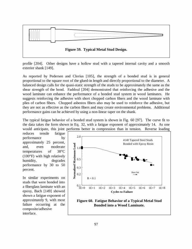
97

profile [204]. Other designs have a hollow stud with a tapered internal cavity and a smoothexterior shank [149].

As reported by Pedersen and Clorius [105], the strength of a bonded stud is in generalproportional to the square root of the glued-in length and directly proportional to the diameter. Abalanced design calls for the quasi-static strength of the studs to be approximately the same as theshear strength of the bond. Faddoul [204] demonstrated that reinforcing the adhesive and thewood laminate can enhance the performance of a bonded stud system in wood laminates. Hesuggests reinforcing the adhesive with short chopped carbon fibers and the wood laminate withplies of carbon fibers. Chopped asbestos fibers also may be used to reinforce the adhesive, butthey are not as effective as the carbon fibers and may create environmental problems. Additionalperformance gains can be achieved by using a non-linear taper on the shank.

The typical fatigue behavior of a bonded stud system is shown in Fig. 60 [97]. The curve fit tothe data takes the form shown in Eq. 32, with a fatigue exponent of approximately 14. As onewould anticipate, this joint performs better in compression than in tension. Reverse loadingreduces tensile fatigueperformance byapproximately 25 percent,and, even moderatetemperatures of 38°C(100°F) with high relativelyhumidity, degradesperformance by 30 to 50percent.

In similar experiments onstuds that were bonded intoa fiberglass laminate with anepoxy, Bach [149] showedshown a fatigue exponent ofapproximately 9, with mostfailure occurring at thecomposite/adhesiveinterface.

Figure 59. Typical Metal Stud Design.

1E+0 1E+1 1E+2 1E+3 1E+4 1E+5 1E+6 1E+7 1E+80.1

0.2

0.3

0.5

1.0

2.0

Cycles to Failure

Nor

mal

ized

Max

imum

Loa

d

Run Out

4140 Tapered Steel StudsBonded with Epoxy Resin

R = 0.1

Figure 60. Fatigue Behavior of a Typical Metal StudBonded into a Wood Laminate.

98

In a recent study, Pedersen and Clorius [105] investigated the residual quasi-static strength ofhollow, tapered bonded studs. These studs were bonded into a Swedish spruce glulam17 blade.The 20-m blade was mounted on a wind turbine for 9 years (the turbine was operated only 3 ofthese 9 years). The authors estimate the studs had endured 5x107 fatigue cycles when the bladewas removed from the turbine because it had been struck by lightning. Based on a sample of 11pull-out tests, the ultimate strength of the stud had been reduced by 5 percent from previouslytested studs of this design. Failures were like a cork pulled from a bottle with all failuresoccurring in the immediate proximity of the wood/adhesive interface. The individual failures wereeither at the interface or a failure in the wood near that interface, with the former dominating.

8.2.4. Adhesives

The reader may note that this section of the paper does not include a detailed discussion of thematerial properties of the adhesive. Unfortunately, this is not an oversight. Rather it reflects alack of material characterizations for typical adhesives that are in the public domain. Althoughsome references are available, e.g. DeLollis [191] and Kinloch [205], only limited properties areavailable and those are usually limited to a single surface preparation and/or primer.

Typically, the designer is forced to develop the required material characterization as part of thedesign process, e.g. see Guess et al. [199], or use proprietary information obtained directly fromthe manufacturer. In most cases, the designer is forced to take a best practice approach and usesupplier specifications and recommendations for the design and manufacturing of the complexjoint structures. And, finally, component tests must be used to qualify the joint.

8.2.5. Comments

Although not proven conclusively, the performance of tubular lap joints appears to be directlyrelated to the peel stress that acts across the adhesive. Because the stresses are singular at eachend of the adhesive, the analysis of these joint systems are difficult at best, and even FEA must beused with extreme care because its predictions are mesh dependent. However, the designer canuse FEA effectively to investigate the geometry of the joint that minimizes these stresses and,thus, maximizes the performance of the joint.

Unfortunately, the quasi-static and fatigue strength of joints typically used for wind turbineapplications cannot be predicted accurately. A fracture mechanics approach based on stressintensity factors has had reasonably good success when geometries are relatively simple. Andwhen combined with specialized finite element analyses, more complex joint structures can beanalyzed, but failure strength typically cannot be predicted accurately. And as the design processfor bonded studs indicates, most bonded joints must be tested to validate design

17 A wood composite created from sheet veneers and epoxy. See the loads discussion in section 5.2.2 “LaminatedWood” on p. 47.

99

8.3. Nondestructive Testing

Nondestructive Testing and Evaluation (NDT and NDE) offer proven techniques for theinspection of structural components. General descriptions of techniques and applications exist inthe literature [206, 207]. As well as applications of these techniques to wind turbines [208-210].

Two techniques that have proven to be especially useful in wind turbine applications are ultrasonictesting and acoustic emissions. The former uses the propagation characteristics of ultrasonic(acoustic) waves to measure material properties throughout the volume of an object. Thistechnique is especially useful for the detection and characterization of surface and subsurfaceflaws. Acoustic emissions (AE) are elastic waves generated by the rapid release of energy fromlocalized sources within a material. By monitoring AE events, typically an array of acoustictransducers is used, information concerning the location and structural significance of the detectedevents can be ascertained.

In the discussion entitled “Tubular Lap Joints” on p. 89, ultrasonic testing techniques [211] areused to detect damage, debonds and cracks in bonded joints that are tested to failure. Thistechnique was extended to the inspection of bonded joints in wind turbine blades [200, 208].

Ultrasonic wave propagation techniques have also been used very successfully to grade veneers,see the discussion entitled “Grading” on p. 47.

Acoustic emissions have shown great promise in detecting the primary failure site of blades, inreal time, while they were being tested in laboratory environments [209, 212]. Of primaryimportance is the ability of this technique to also identify areas of secondary damage. These areareas of high damage that typically do not fail during the test, and, therefore, are difficult orimpossible to locate. They are important to designers because they identify weak points in theblade design. These sites will probably be the location of blade failures if the primary failure site isreinforced. Or, if the failure mechanism changes under field loads, these secondary sites maybecome primary failure sites.

Wei et al. [213] have used acoustic emissions to follow the damage of composite coupons underlaboratory testing.

Additional applications of standard and non-standard NDT and NDE techniques to wind turbinecomponents, in both laboratory and field environments, have been explored [209, 210, 214, 215].

100

8.4. Full Scale Testing

Once the design of a wind turbine blade has been completed and the turbine has been built, thereis no guarantee that it will perform as intended. These highly complicated structures aresusceptible to size effects, manufacturing variations, and inadequate designs. The only real testsof a blade design are through rigorous testing of the blade in a laboratory environment and on anoperating wind turbine.

Musial et al. [81] and Musial and Allread [216] discuss full-blade testing in a laboratoryenvironment. An IEC committee is currently developing a set of recommended practices for thefull-scale testing of turbine blades [217]. Their guide identifies commonly accepted practices andprovides guidance in establishing blade test criteria. Although outside the scope of this report,these testing techniques should be taken into consideration and used as a very important tool inthe design of wind turbine blades.

101

9. CONCLUDING REMARKS

Wind turbines are fatigue critical structures that require detailed analyses to ensure survival undernormal operating conditions in a turbulent environment. While these designs are difficult, they arenot impossible. The research of the past few years provides the designer with most of the toolsand knowledge to address design problems with a high degree of confidence. Some questionshave yet to be answered, but research is ongoing. This paper was intended to guide the windturbine designer through the issues that affect fatigue performance of turbine components and todescribe best practices when appropriate.

103

10. REFERENCES

1. Righter, R.W., Wind Energy in America, A History, University of Oklahoma Press,Norman, 1996.

2. Baker, T.L., Blades in the Sky, Texas Tech University Press, Lubbock, 1992.

3. Hunt, V.D., Windpower: A Handbook on Wind Energy Conversion Systems, Van NostrandReinhold Co., New York, 1981.

4. Eggleston, D.M., and F.S. Stoddard, Wind Turbine Engineering Design, Van NostrandReinhold, New York, 1987.

5. Freris, L.L., ed., Wind Energy Conversion Systems, Prentice Hall, New York, 1990.

6. Spera, D.A., ed., Wind Turbine Technology, ASME Press, New York, 1994.

7. Walker, J.F., and N. Jenkins, Wind Energy Technology, John Wiley & Sons, Chichester,1997.

8. Miner, A.A., “Cumulative Damage in Fatigue,” Trans. ASME, Vol. 67, 1945, p. A159.

9. Rice, R.C., et al., Fatigue Design Handbook, SAE, Second Edition, 1988.

10. Osgood, C.C., Fatigue Design, Second Edition, Pergamon Press, New York, 1982.

11. Fuchs, H.O., and R.I. Stephens, Metal Fatigue in Engineering, Wiley & Sons, New York,1980.

12. Lampman, S.R., ed., ASM Handbook, Vol. 19: Fatigue and Fracture, ASM Int., MaterialsPark, OH, 1996.

13. Hertzberg, R.W., Deformation and Fracture Mechanics of Engineering Materials, Wiley,New York, 1977.

14. Kanninen, M.F., and C.H. Popelar, Advanced Fracture Mechanics, Oxford UniversityPress, New York, 1985.

15. Sutherland, H.J., P.S. Veers and T.D. Ashwill, “Fatigue Life Prediction for Wind Turbines:A Case Study on Loading Spectra and Parameter Sensitivity,” Case Studies for FatigueEducation, ASTM STP 1250, R. I. Stephens, ed., 1994, p. 174.

16. Kensche, C.W., ed., Fatigue of Materials and Components for Wind Turbine Rotor Blades,EUR 16684, European Commission, Luxembourg, 1996.

104

17. Wind Turbine Generator systems - Part 1: Safety Requirements, IEC 61400-1, prepared byIEC-TC88, 1998.

18. Veers, P.S., “Simplified Fatigue Damage and Crack Growth Calculations for WindTurbines,” Eighth ASME Wind Energy Symposium, D.E. Berg and P.C. Klimas, eds., SED-Vol.7, ASME, 1989, p. 133.

19. Sutherland, H.J., and L.L. Schluter, “The LIFE2 Computer Code, Numerical Formulationand Input Parameters,” Proceedings of WindPower '89, SERI/TP-257-3628, September 1989, p.37.

20. Sutherland, H.J., and L.L. Schluter, “Crack Propagation Analysis of WECS Componentsusing the LIFE2 Computer Code,” Eighth ASME Wind Energy Symposium, D.E. Berg and P.C.Klimas, eds., SED-Vol. 7, ASME, 1989, p. 141.

21. Sutherland, H.J., “Damage Predictions for Wind Turbine Components Using the LIFE2Computer Code,” Proceedings of EWEC '89, Peter Peregrinus Ltd, 1989, p. 384.

22. Butterfield, C.P., C. Stork, W. Holley, P.H. Madsen, and P.H. Jensen, “External ConditionModels from the International Electrotechnical Commission Safety of Wind Turbine Standards(1400-1),” 1997 ASME Wind Energy Symposium, AIAA/ASME, W. Musial and D.E. Berg, eds.,1997, p. 65.

23. Akins, R. E., “Cross-Spectral Measurements in the Testing of Wind Turbines,” Ninth ASMEWind Energy Symposium, D. E. Berg, ed., SED-Vol. 9, ASME, 1990, p. 155.

24. European Wind Turbine Standards, Vol. 2: Load Spectra for Wind Turbine Design,EUREC-Agency, Joule II Programme, contr: JOU2-CT93-0387, Final Draft, 1996.

25. Madsen, P.H., ed., Recommended Practices for Wind Turbine Testing and Evaluation, Vol.3 - Fatigue Loads, 1990, International Energy Agency, 1990.

26. “State of the Art of Aeroelastic Codes for Wind Turbine Calculations,” 28th Meeting ofExperts, ISSN 0590-8809, IEA, B.M. Pedersen, ed., Lyngby, Denmark, 1996.

27. Downing, S.D., and D.F. Socie, “Simple Rainflow Counting Algorithms,” InternationalJournal of Fatigue, Vol. 4, N. 1, 1982, p. 31.

28. Sutherland, H.J. and L.L. Schluter, “Fatigue Analysis of WECS Components Using aRainflow Counting Algorithm,” Proceedings of Windpower '90, AWEA, Washington, DC, 1990,p. 85.

29. Wu, K.C., and S. Kammula, “A New On-Line, Real-Time RainFlow Counting Algorithm,”Wind Energy: Energy Week, ASME/API, 1996, p. 132.

105

30. Veers, P.S., S.R. Winterstein, D.N. Nelson, and C.A. Cornell, “Variable Amplitude LoadModels for Fatigue Damage and Crack Growth,” Development of Fatigue Loading Spectra,ASTM STP 1006, J.M. Potter and R.T. Watanabe, eds., 1989, p. 172.

31. Wind Turbine Generator Systems, Part 13: Measurement of Mechanical Loads, DraftTechnical Report, IEC 61400-13, prepared by IEC-TC88, Working Group 11, 1998.

32. Coleman, C., and B. McNiff, Final Report: Dynamic Response Testing of the Northwind100 Wind Turbine, Subcontractor Report, SERI Cooperative Research Agreement #DE-FC02-86CH10311, Solar Energy Research Institute, Golden, CO, 1989.

33. Sutherland, H.J., “Frequency Domain Analysis of the Fatigue Loads on Typical WindTurbine Blades,” J. of Solar Energy Engineering, Transactions of ASME, Vol. 118, 1996, p. 204.

34. Sutherland, H.J., “Frequency-Domain Stress Prediction Algorithm for the LIFE2 FatigueAnalysis Code,” Eleventh ASME Wind Energy Symposium, P.S. Veers and S.M. Hock, eds.,SED-Vol. 12, ASME, 1992, p. 107.

35. Bishop, N.W.M. and F. Sherratt, “A Theoretical Solution for the Estimation of ‘Rainflow’Ranges from Power Spectral Density Data,” Fatigue and Fracture of Engineering Materials andStructures, Vol. 13, No. 4, 1990, p. 311.

36. Bishop, N.W.M., “Using Frequency Domain Methods to Predict Structural Fatigue of WindTurbine Blades,” 23rd Meeting of Experts – Fatigue of Wind Turbines, IEA, M. Pedersen, ed.,Golden, Colorado, 1992, p. 89.

37. Akins, R.E., “Rainflow Counting Based on Predicted Stress Spectra,” Eighth ASME WindEnergy Symposium, D.E. Berg and P.C. Klimas, eds., SED-Vol. 7, ASME, 1989, p. 131.

38. Akins, R.E., “Rainflow Counting Based on Predicted Stress Spectra,” Seventh ASME WindEnergy Symposium, A.H.P. Swift and R.W. Thresher, eds., SED-Vol. 5, ASME, 1988, p. 159.

39. Ashwill, T.D., D.E. Berg, L.R. Gallo, R.D. Grover, P.C. Klimas, M.E. Ralph, M.A.Rumsey, W.A. Stephenson, and H.J. Sutherland, “The Sandia 34-Meter VAWT Test Bed,”Proceedings of Wind Power '87, American Wind Energy Association, SERI/CP-217-3315, 1987,p. 298.

40. Sutherland, H.J., and R.M. Osgood, “Frequency-Domain Synthesis of the Fatigue LoadSpectrum for the NPS 100-kW Wind Turbine,” Proceedings of WindPower '92, American WindEnergy Association, Washington, DC, 1992, p. 321.

41. Malcolm, D.J., Fatigue Life Assessment of VAWT Components, Indal Technologies,Mississauga, 1985.

106

42. Malcolm, D.J., “Predictions of Peak Fatigue Stresses in a Darrieus Rotor Wind TurbineUnder Turbulence Winds,” Ninth ASME Wind Energy Symposium, D. E. Berg, ed., SED-Vol. 9,ASME, 1990, p. 125.

43. Veers, P.S., An Approach to the Fatigue Analysis of Vertical Axis Wind Turbine Blades,SAND81-2130, Sandia National Labs, Albuquerque, NM, 1981.

44. Veers, P.S., “Blade Fatigue Life Assessment with Application to VAWTs,” J. SolarEngineering, Vol. 104, 1982, p. 106.

45. Veers, P.S., A General Method for Fatigue Analysis of Vertical Axis Wind Turbine Blades,SAND82-2543, Sandia National Laboratories, Albuquerque, NM, 1983.

46. Akins, R.E., “Wind Turbine Fatigue Measurement Techniques,” Sixth ASME Wind EnergySymposium, R.W. Thresher, ed., SED-Vol. 3, ASME, 1987, p. 147.

47. Jackson, K.L., “Deriving Fatigue Design Loads from Field Test Data,” Wind Power ‘92,AWEA, 1992, p. 313.

48. Jackson, K.L., “A Method of Fatigue Life Assessment of Wind Turbine Structures,” WindEnergy - 1993, S. Hock, ed., SED-Vol. 14, ASME, 1993, p. 179.

49. Kelley, N.D. “The Identification of Inflow Fluid Dynamics Parameters That Can be Used toScale Fatigue Loading Spectra of Wind Turbine Structural Components,” Wind Energy - 1994,W.D. Musial, S.M. Hock, and D.E. Berg, eds., SED-Vol. 15, ASME, 1994, p. 181.

50. Kelley, N.D., Turbulence Descriptors for Scaling Fatigue Loading Spectra of Wind TurbineStructural Components, NREL/TP-442-7035, NREL, Golden, 1994.

51. Kelley, N.D., and H.E. McKenna, “The Evaluation of a Turbulent Loads CharacterizationSystem,” Wind Energy: Energy Week, ASME/API, 1996, p. 69.

52. Winterstein, S.R., and C.H. Lange, “Load Models for Fatigue Reliability from LimitedData,” Wind Energy - 1995, W.D. Musial, S.M. Hock and D.E. Berg, eds., SED-Vol. 16, ASME,1995, p. 73.

53. Winterstein, S.R., C.H. Lange, and S. Kumar, FITTING: A Subroutine to Fit Four MomentProbability Distributions to Data, Rept. RMS-14, Rel. Marine Struc. Prog., Civil Eng. Dept.,Stanford University, Stanford, CA, 1995.

54. Winterstein, S.R., and T. Kashef, “Moment-Based Load and Response Models with WindEngineering Applications,” 1999 Wind Energy Symposium, AIAA/ASME, 1999, p. 346.

55. Sutherland, H.J., and C.P. Butterfield, “A Summary of the Workshop on Fatigue LifeMethodologies for Wind Turbines,” Proceedings of WindPower ‘94, AWEA, Washington, DC,1994, p. 279.

107

56. Ashwill, T.D., and P.S. Veers, “Structural Response Measurements and Predictions for theSandia 34-Meter Test Bed,” Ninth ASME Wind Energy Symposium, D. E. Berg, ed., SED-Vol. 9,ASME, 1990, p. 137.

57. Ashwill, T.D., H.J. Sutherland, and P.S. Veers, “Fatigue Analysis of the Sandia 34-MeterVertical Axis Wind Turbine,” Ninth ASME Wind Energy Symposium, D. E. Berg, ed., SED-Vol.9, ASME, 1990, p. 145.

58. Lange, C.H., and S.R. Winterstein, “Fatigue Design of Wind Turbine Blades: Load andResistance Factors from Limited Data,” Wind Energy: Energy Week, ASME/API, 1996, p. 93.

59. Kashef, T., and S.R. Winterstein, “Relating Turbulence to Wind Turbine Blade Loads:Parametric Study with Multiple Regression Analysis,” 1998 ASME Wind Energy Symposium, W.Musial and D.E. Berg, eds., AIAA/ASME, 1998, p. 273.

60. Veers, P.S., and S.R. Winterstein, “Application of Measured Loads to Wind Turbine Fatigueand Reliability Analysis,” Journal of Solar Energy Engineering, ASME, Vol. 120, 1998, p. 233.

61. Sutherland, H.J., and P.S. Veers, “Effects of Cyclic Stress Distribution Models on FatigueLife Predictions,” Wind Energy - 1995, W.D. Musial, S.M. Hock and D.E. Berg, eds., SED-Vol.16, ASME, 1995, p. 83.

62. Kelley, N.D., and H.J. Sutherland, “Damage Estimates from Long-Term Structural Analysisof a Wind Turbine in a U.S. Wind Farm Environment,” 1997 ASME Wind Energy Symposium,AIAA/ASME, W. Musial and D.E. Berg, eds., 1997, p. 170.

63. Veers, P.S., “Three-Dimensional Wind Simulation,” Eighth ASME Wind EnergySymposium, D.E. Berg and P.C. Klimas, eds., SED-Vol. 7, ASME, 1989, p. 23.

64. Veers, P.S., Modeling Stochastic Winds on Vertical Axis Wind Turbines, SAND88-0152,Sandia National Laboratories, Albuquerque, NM, 1988.

65. Kelley, N.D., “Full Vector (3-D) Inflow Simulation in Natural and Wind Farm EnvironmentsUsing an Expanded Version of the SNLWIND (Veers) Turbulence Code,” Wind Energy - 1993,S. Hock, ed., SED-Vol. 14, ASME, 1993, p. 77.

66. Cuerva-Tejero, A., S. López-Díez, and D. Bercebal-Weber, “Higher Level Descriptors ofSites and Wind Turbines by Means of Principal Components Analysis,” Proceedings of 1999EWEC, 1999, in publication.

67. Thresher, R.W., S.M. Hock, and R.M. Osgood, “Data Record Length Effects on RainflowAnalysis,” Eleventh ASME Wind Energy Symposium, P.S. Veers and S.M. Hock, eds., SED-Vol.12, ASME, 1992, pp. 117.

68. Jackson, K.L., “Scaling Wind Turbine Fatigue Design Loads,” Wind Energy - 1994, W.D.Musial, S.M. Hock, and D.E. Berg, eds., SED-Vol. 15, ASME, 1994, p. 189.

108

69. Spera, D.A., “A Model of Rotationally-Sampled Wind Turbulence for Predicting FatigueLoads in Wind Turbines of the Scale and Type of the NASA/DOE Mod-2 HAWT,” WindEnergy: Energy Week, ASME/API, 1996, p. 59.

70. Barnard, J.C., and L.L. Wendell, “A Simple Method of Estimating Wind Turbine BladeFatigue at Potential Wind Turbine Sites,” J. of Solar Energy Engineering, Transactions ofASME, Vol. 119, ASME, 1997, p. 174.

71. Mann, J., “Wind Field Simulation,” Probabilistic Engineering Mechanics, Elsevier ScienceLTD, Vol. 13, No. 4, 1998, p. 269.

72. Wilson, R.E., S.N. Walker, C.E. Smith and L.N. Freeman, “Advanced Dynamics Code,”Wind Energy - 1993, S. Hock, ed., SED-Vol. 14, ASME, 1993, p. 119.

73. Hansen, A.C., Yaw Dynamics of Horizontal Axis Wind Turbines: Final Report, TP 442-4822, NREL, Golden, 1992.

74. Elliott, A.S., and A.D. Wright, “ADAMS/WT: An Industry-Specific Interactive ModelingInterface for Wind Turbine Analysis," Wind Energy - 1995, W.D. Musial, S.M. Hock and D.E.Berg, eds., SED-Vol. 16, ASME, 1995, p. 111.

75. Quarton, D.C., “The Evolution of Wind Turbine Design Analysis – A Twenty Year ProgressReview,” Wind Energy, Vol. 1, Spring 1998, p. 5.

76. Wilson, R.E., T.L. Weber and S.N. Walker, “Prediction of Fatigue Loads on a Free-YawHAWT,” Eleventh ASME Wind Energy Symposium, P.S. Veers and S.M. Hock, eds., SED-Vol.12, ASME, 1992, pp. 71.

77. Laino, D.J., and A.C. Hansen, “A Fatigue Analysis Interface for YawDyn and ADAMS,”Wind Energy: Energy Week, ASME/API, 1996, p. 23.

78. Hansen, A.C., and D.J. Laino, “Validation Study for AeroDyn and YawDyn Using Phase IIICombined Experiment Data,” 1997 ASME Wind Energy Symposium, AIAA/ASME, W. Musialand D.E. Berg, eds., 1997, p. 109.

79. Laino, D.J., and A.C. Hansen, “Sources of Fatigue Damage to Wind Turbine Blades,” 1998ASME Wind Energy Symposium, AIAA/ASME, W. Musial and D.E. Berg, eds., 1998, p. 304.

80. Mouzakis, F., and E. Morfiadakis, “Identification of Low Cycle Effects on Wind TurbineComponent Lifetime Estimation,” BWEA ’97.

81. Musial, W., M. Clark, N. Egging and M. Zuteck, “A Comparison of Strength and Load-Based Methods for Testing Wind Turbine Blades,” 1997 ASME Wind Energy Symposium,AIAA/ASME, W. Musial and D.E. Berg, eds., 1997, p. 228.

109

82. Wu, K.C., and R. De La Guardia, “The Effects of Controls on Fatigue Loads in Two-BladedTeetered Rotor Wind Turbines,” Wind Energy: Energy Week, ASME/API, 1996, p. 102.

83. McNiff, B.P., W.D. Musial, and R. Errichello, “Variations in Gear Fatigue Life for DifferentWind Turbine Braking Strategies,” Proceedings of Windpower '90, AWEA, Washington, DC,1990, p. 131.

84. Larsen, G. and Thomsen, K., “A Simple Approximative Procedure for Talking into AccountLow Cycle Fatigue Loads,” Proc. IEA 4th Symposium of Wind Turbine Fatigue, IEA, 1996.

85. Sutherland, H.J., “Effect of the Flap and Edgewise Bending Moment Phase Relationships onthe Fatigue Loads of a Typical HAWT,” Wind Energy - 1993, S. Hock, ed., SED-Vol. 14,ASME, 1993, p. 181.

86. Zuteck, M.D., “A Methodology for Combined Loading Fatigue Calculations,” Wind Energy- 1994, W.D. Musial, S.M. Hock, and D.E. Berg, eds., SED-Vol. 15, ASME, 1994, p. 205.

87. Timoshenko, S., Strength of Materials, C. Van Nostrand Co., Princeton, 1955.

88. Ten Have, A.A., WISPER and WISPERX: Final Definition of Two Standardized FatigueLoading Sequences for Wind Turbine Blades, NLR-TP-91476U, National Aerospace LaboratoryNLR, Amsterdam, the Netherlands, 1992.

89. Ten Have, A.A., “WISPER and WISPERX: A Summary Paper Describing TheirBackgrounds, Derivation and Statistics,” Wind Energy - 1993, S. Hock, ed., SED-Vol. 14,ASME, 1993, p. 169.

90. Kelley, N.D., “A Comparison of Measured Wind Park Load Histories With The WISPERand WISPERX Load Spectra,” Wind Energy 1995, Musial, Hock and Berg, eds., SED-Vol. 16,ASME, 1995, p. 107.

91. Tangler, J., B. Smith, D. Jager, and T. Olsen, Atmospheric Performance of the SERI Thin-Airfoil Family, SERI/TP-257-3939, Solar Energy Research Institute, Golden, CO, 1990.

92. Tangler, J., N.D. Kelley, D. Jager and B. Smith, “Measured Structural Loads for the Micon65/13,” Wind Energy - 1994, W.D. Musial, S.M. Hock, and D.E. Berg, eds., SED-Vol. 15,ASME, 1994, p. 197.

93. Sutherland, H.J., and N.D. Kelley, “Fatigue Damage Estimate Comparisons for NorthernEuropean and U.S. Wind Farm Loading Environments,” Proceedings of WindPower ‘95, AWEA,Washington, DC, 1995, pp. 177.

94. Thomsen, K. and S.M. Petersen, Experimental Investigation of Gear Box DurationLoadings on Stall and Pitch Controlled Wind Turbines, Riso-R-653(EN), RISO, Roskilde,Denmark, 1992.

110

95. Sutherland, H.J. and D.P. Burwinkle, “The Spectral Content of the Torque Loads on aTurbine Gear Tooth,” Wind Energy - 1995, W.D. Musial, S.M. Hock and D.E. Berg, eds., SED-Vol. 16, ASME, 1995, p. 91.

96. AGMA/AWEA 921-A97, Recommended Practices for Design and Specification ofGearboxes for Wind Turbine Generator Systems, American Gear Manufacturers Association,Alexandria, VA, 1997.

97. Spera, D.A., J.B. Esgar, M. Gougeon, and M.D. Zuteck, Structural Properties ofLaminated Douglas Fir/Epoxy Composite Material, DOE/NASA Reference Publication 1236,DOE/NASA/20320-76, Cleveland, 1990.

98. Handbook of Fatigue Testing, S.R. Swanson, ed., ASTM STP 566, Philadelphia, 1974.

99. Forman, R.G., V. Shivakumar and J.C. Newman, Fatigue Crack Growth ComputerProgram: “NASA/FLAGRO,” NASA, JSC-22267, Houston, 1986.

100. Forman, R.G., Derivation of Crack Growth Properties of Materials for NASA/FLAGRO,NASA, Materials Branch Report 86-ES5-1, Houston, 1986.

101. Wood Handbook: Wood as an Engineering Material, Forest Product Laboratory, U.S.Dept. of Agriculture, Agriculture Handbook 72, Washington, 1987.

102. Jung, J., Stress Wave Grading Techniques on Veneer Sheets, Forest Products Laboratory,General Technical Report FPL-27, Madison, 1979.

103. Jung, J., “Properties of Parallel-Laminated Veneer From Stress-Wave-Tested Veneers,”Forest Products Journal, vol. 32, no. 7, 1982, pp. 30.

104. Jamieson, P., “The Design of Wood Epoxy Wind Turbine Blades,” Eighth ASME WindEnergy Symposium, D.E. Berg and P.C. Klimas, eds., SED-Vol. 7, ASME, 1989, p. 147.

105. Pedersen, M.U., and C.O. Clorius, The Strength of Glued-in Bolts after 9 Years In SituLoading, Technical University of Denmark, DK9601314, NEI-DK-2303, 1995.

106. Stipe, C., W. Musial, M. Jenks, and S. Hughes, Static Ramp and Compression-Compression Fatigue Testing of Sitka Spruce Specimens, National Renewable EnergyLaboratory, Golden, 1999.

107. Bonfield, P.W. I.P. Bond, C.L. Hacker and M.P. Ansell, “Fatigue Testing of WoodComposites for Aerogenerator Blades. Part VII, Alternative Wood Species and Joints”, WindEnergy Conversion, B.R. Clayton, ed., Mechanical Engineering Publications Ltd., 1992, p. 243.

108. Boyer, H.E., and T.L. Gall, eds., Metals Handbook, Desk Edition, American Society forMetals, Metals Park, Ohio, 1985.

111

109. Aluminum Standard and Data, 1984, Eighth Edition, The Aluminum Association,Washington, DC, 1984.

110. Boyer, H.E., ed., Atlas of Stress-Strain Curves, American Society for Metals, Metals Park,Ohio, 1985.

111. Boyer, H.E., ed., Atlas of Fatigue Curves, American Society for Metals, Metals Park, Ohio,1985.

112. Peterson, R.E., Stress Concentration Factors, Charts and Relations Useful in MakingStrength Calculations for Machine Parts and Structural Elements, Wiley IntersciencePublication, New York, 1974.

113. Hoeppner, D.W., ed., Fatigue Testing of Weldments, STP 648, American Society forTesting and Materials, Philadelphia, 1977.

114. Alcoa Industries working with SNL engineers in mid 1970s: see, Kadlec, E.G.,Characteristics of Future Vertical Axis Wind Turbines, SAND79-1068, Sandia NationalLaboratories, Albuquerque, NM, 1982.

115. Berg, D.E., P.C. Klimas, and W.A. Stephenson, “Aerodynamic Design and InitialPerformance Measurements for the Sandia 34-m Diameter Vertical-Axis Wind Turbine,” NinthASME Wind Energy Symposium, D. E. Berg, ed., SED-Vol. 9, ASME, 1990, p. 85.

116. Van Den Avyle, J.A., and H.J. Sutherland, “Fatigue Characterization of a VAWT BladeMaterial,” Eighth ASME Wind Energy Symposium, D.E. Berg and P.C. Klimas, eds., SED-Vol. 7,ASME, 1989, p. 125.

117. Mitchell, M. R., “Fundamentals of Modern Fatigue Analysis,” Fatigue and Microstructure,ASM Material Science Seminar, St. Louis, MO, 1978, American Society for Metals, 1979.

118. Rolfe, S.T., and J.M. Barsom, “Fracture and Fatigue Control in Structures,” Applications ofFracture Mechanics, Prentice-Hall, 1977, p. 244.

119. Hatch, P.W., J.A. Van Den Avyle and J. Laing, Fatigue Crack Growth Automated TestingMethod, SAND89-0778 Sandia National Laboratories, Albuquerque, 1989.

120. Warren, A.S. and R.M. Pelloux, Fatigue Behavior of 6063 Aluminum Alloy Extrusions forWind Turbine Applications, Final Report, SNL Contract No. 33-7708, MIT, Cambridge, 1990.

121. Veers, P.S., and J.A. Van Den Avyle, “Fatigue Crack Growth from Narrow-Band GaussianSpectrum Loading in 6063 Aluminum Alloy,” Advances in Fatigue Lifetime PredictiveTechniques, ASTM STP 1122, M.R. Mitchell and R.W. Landgraf, eds., ASTM, Philadelphia,1992, p. 191.

112

122. AGMA Standard, Standard - Design Guide for Vehicle Spur and Helical Gears, AGMA170.01-1976, American Gear Manufacturers Association, Alexandria, VA, 1976.

123. AGMA Information Sheet, Geometry Factors for Determining the Pitting Resistance andBending Strength of Spur, Helical and Herringbone Gear Teeth, AGMA 908-B89, AmericanGear Manufacturers Association, Alexandria, VA, 1989.

124. Composites, Engineered Materials Handbook, Vol. 1, ASM, T.J. Reinhart, Tech. Chair.,Materials Park, OH, 1998.

125. Tsai, S.W., and H.T. Hahn, Introduction to Composite Materials, Technomic PublishingCo., Inc., 1980.

126. Mayer, R.M., ed., Design of Composite Structures Against Fatigue: Applications to WindTurbine Blades, Mechanical Engineering Publications, United Kingdom, 1996.

127. Mandell, J.F. and D.D. Samborsky, DOE/MSU Composite Materials Fatigue Database:Test Methods, Materials, and Analysis, SAND97-3002, Sandia National Laboratories,Albuquerque, 1997.

128. De Smet, B.J., and P.W. Bach, Database FACT: Fatigue of Composite for wind Turbines,ECN-C-94-045, ECN, Petten, 1994.

129. Mandell, J.F., R.M. Reed Jr., and D.D. Samborsky, Fatigue of Fiberglass Wind TurbineBlade Materials, Contractor Report SAND92-7005, Sandia National Laboratories, Albuquerque,NM, 1992.

130. Mandell, R.M., J.F. Reed Jr., D.D. Samborsky and Q. Pan, “Fatigue Performance of WindTurbine Blade Materials,” Wind Energy - 1993, S. Hock, ed., SED-Vol. 14, ASME, 1993, p.191.

131. Mandell, J.F., R.M. Creed Jr., Q. Pan, D. W. Combs and M. Shrinivas, “Fatigue ofFiberglass Generic Materials and Substructures,” Wind Energy - 1994, W.D. Musial, S.M. Hock,and D.E. Berg, eds., SED-Vol. 15, ASME, 1994, p. 207.

132. Mandell, J.F., D.W. Combs and D.D. Samborsky, “Fatigue of Fiberglass BeamSubstructures,” Wind Energy - 1995, W.D. Musial, S.M. Hock and D.E. Berg, eds., SED-Vol.16, ASME, 1995, p. 99.

133. Samborsky, D.D. and J. F. Mandell, “Fatigue Resistant Fiberglass Laminates for WindTurbine Blades,” Wind Energy: Energy Week, ASME/API, 1996, p. 46.

134. Cairns, D.S., J.F. Mandell, M.E. Scott, and J.Z. Macagnano, “Design Considerations for PlyDrops in Composite Wind Turbine Blades,” 1997 ASME Wind Energy Symposium,AIAA/ASME, W. Musial and D.E. Berg, eds., 1997, p. 197.

113

135. Shrinivas, M., Three Dimensional Finite Element Analysis of Matrix Cracks inMultidirectional Composite Laminates, M.S. Thesis, Dept. of Chem. Engr., Montana StateUniversity, 1993.

136. Samborsky, D.D., J.F. Mandell and D.S. Cairns, “Selection of Reinforcing Fabrics for WindTurbine Blades,” 1999 Wind Energy Symposium, AIAA/ASME, 1999, p. 32.

137. Mandell, J.F., D.D. Samborsky and H.J. Sutherland, “Effects of Materials Parameters andDesign Details on the Fatigue of Composite Materials for Wind Turbine Blades,” Proceedings of1999 EWEC, 1999, in publication.

138. Van Delft, D.R.V., G.D. de Winkel, and P.A. Josses, “Fatigue Behavior of Fibreglass WindTurbine Blade Material Under Variable Amplitude Loading,” 1997 ASME Wind EnergySymposium, AIAA/ASME, W. Musial and D.E. Berg, eds., 1997, p. 180.

139. Mandell, J.F., “Fatigue Behavior of Short Fiber Composite Materials,” The FatigueBehavior of Composite Materials, K.L. Reifsnider, ed., Elsevier, 1991, p. 232.

140. Mohamadian, H.P., and I.J. Graham, “Stiffness Degradation In Unidirectional + ChoppedMat E-Glass Fiber/Polyester and Vinylester Composite Laminates,” Tenth ASME Wind EnergySymposium, D.E. Berg and P.S. Veers, eds., SED-Vol. 11, ASME, 1991, p. 55.

141. Sutherland, H.J., and J.F. Mandell, “Application of the U.S. High Cycle Fatigue Data Baseto Wind Turbine Blade Lifetime Predictions,” Wind Energy: Energy Week, ASME/API, 1996, p.85.

142. Van Delft, D.R.V., P.A. Joosse and H.D. Rink, “Fatigue Behavior of Fibreglass WindTurbine Blade Material at the Very High Cycle Range,” Proceedings of EWEC ’94, 1994, p. 379.

143. De Winkel, G.D., and D.R.V. Van Delft, Fatigue Behavior of Glass Fibre ReinforcedPolyester for Wind Turbine Blades; Part 2: Fatigue Behavior under the WISPER and WISPERXVariable Amplitude Loading, Stevin Report 6-96-20, Delft University of Technology, Delft, TheNetherlands, 1996.

144. Echtermeyer, A.T., C. Kensche, P. Bach, M. Poppen, H. Lilholt, S.I. Andersen and P.Brøndsted, “Method to Predict Fatigue Lifetimes of GRP Wind Turbine Blades and Comparisonwith Experiments,” Proceedings of the European Union Wind Energy Conference, Göteborg,Sweden, 1996, p. 907.

145. Mandell, J., D. Samborsky and D. Cairns, “Advanced Wind Turbine Blade StructureDevelopment Program at Montana State University,” 1997 ASME Wind Energy Symposium,AIAA/ASME, W. Musial and D.E. Berg, eds., 1997, p. 189.

114

146. Mandell, J., D. Samborsky, M. Scott and D. Cairns, “Effects of Structural Details onDelamination and Fatigue Life of Fiberglass Laminates,” 1998 ASME Wind Energy Symposium,AIAA/ASME, W. Musial and D.E. Berg, eds., 1998, p. 323.

147. Cairns, D., D. Haugen, J. Mandell and D. Samborsky, “Fracture of Skin/StiffenerIntersections in Composite Wind Turbine Structures,” 1998 ASME Wind Energy Symposium,AIAA/ASME, W. Musial and D.E. Berg, eds., 1998, p. 334.

148. Mandell, J.F., D.D. Samborsky, D.W. Combs, M.E. Scott and D.S. Cairns, Fatigue ofComposite Material Beam Elements Representative of Wind Turbine Blade Substructure,NREL/SR-500-24379, National Renewable Energy Laboratory, Golden, CO, 1998.

149. Bach, P.W., Fatigue of Stud Joints for GFRP Wind Turbine Blades, ECN-C95-117, ECN,Petten, the Netherlands, 1995.

150. De Bruijn, J.C.M., J.A. ter Laak and C.A.M. van den ENDE, “EN-WISPER,” Proceedingsof the IEA Third Symposium of Wind Turbine Fatigue, IEA, Implementing Agreement for aProgramme of Research and Development on Wind Energy Conversion Systems - Annex XI,1994, pp. 55.

151. De Bruijn, J.C.M., EN-WISPER: Environmental Influence on the Fatigue Behavior of WindTurbine Rotor Blades, 50950-KIM 95-9313, KEMA, Arnhem, 1995.

152. Mandell, J.F., Montana State University, Bozeman, personal communication to the author.

153. Joosse, P.A., “EN-WISPER: Research Overview and Consequences,” Proceedings of theIEA Third Symposium of Wind Turbine Fatigue, IEA, Implementing Agreement for a Programmeof Research and Development on Wind Energy Conversion Systems - Annex XI, 1996, p. 87.

154. Joose, P.A. and D.R.V. van Delft, “Has Fatigue Become a Wearisome Subject?,”Proceeding of the European Union Wind Energy Conference, Göteborg, Sweden, 1996, p. 902.

155. Rohatgi, J.S., and V. Nelson, Wind Characteristics: An Analysis for the Generation ofWind Power, Alternative Energy Institute, West Texas A&M University, Canyon, TX, 1994.

156. Elliott, D.L., et al., Wind Energy Resource Atlas of the United States, DOE/CH 10093-4,SERI, Golden, CO, 1987.

157. Schwartz, M.N. and D.L. Elliott, “Mexico Wind Resource Assessment Project,”Proceedings of Windpower '95, AWEA, Washington, DC, 1995, p. 56.

158. Mouzakis, F., E. Morfiadakis and P. Dellaportas, “Fatigue Loading ParametersIdentification of a Wind Turbine Operating in Complex Terrain,” submitted for publication.

159. Mouzakis, F., E. Morfiadakis and A. Fragoulis, Mounturb Final Report, Contract No.JOU2-CT93-0378, Center for Renewable Energy Sources, Pikermi, Greece, 1996.

115

160. Fragoulis, A.N., “The Complex Terrain Wind Environment and Its Effects on the PowerOutput and Loading of Wind Turbines,” 1997 ASME Wind Energy Symposium, AIAA/ASME,W. Musial and D.E. Berg, eds., 1997, p. 33.

161. Voutsinas, S., V. Riziotis and P. Chaviaropoulos, “Non-Linear Aerodynamics and FatigueLoading on Wind Turbines,” 1997 ASME Wind Energy Symposium, AIAA/ASME, W. Musialand D.E. Berg, eds., 1997, p. 41.

162. Veers, P.S., C.H. Lange and S.R. Winterstein, “FAROW: A Tool for Fatigue and Reliabilityof Wind Turbines,” Proceedings of Windpower ’93, AWEA, Washington, DC, 1993, p. 342.

163. Veers, P.S., S.R. Winterstein, C.H. Lange and T.A. Wilson, FAROW: Fatigue andReliability of Wind Turbine Components, SAND94-2460, Sandia National Laboratories,Albuquerque, NM, 1994.

164. Ashwill, T.D., and N. Slack, “Fatigue Life Prediction for Vertical Axis Wind Turbine BladesUsing the LIFE Computer Program,” Internal Memorandum, Sandia National Laboratories,Albuquerque, NM, 1986.

165. Akins, R.E., Initial Analysis of Structural Data: DAF 6400 Rotor, Washington and LeeUniversity, Lexington, 1985.

166. Malcolm, D.J., Fatigue Life Assessment of VAWT Components, Indal Technologies,Mississauga, 1985.

167. Sutherland, H.J., T.D. Ashwill and N. Slack, The LIFE Computer Code Fatigue LifePrediction for Vertical Axis Wind Turbine Components, SAND87-0792, Sandia NationalLaboratories, Albuquerque, NM, 1987.

168. Sutherland, H.J., and T. D. Ashwill, “Fatigue Life Prediction for VAWT Components Usingthe LIFE Codes,” Sixth ASME Wind Energy Symposium, R.W. Thresher, ed., SED-Vol. 3,ASME, 1987, p. 193.

169. Sutherland, H. J., T. D. Ashwill, and K. A. Naassan, “Fatigue Analysis Codes for WECSComponents,” Proceedings of Wind Power '87, SERI/CP-217-3315, AWEA, Washington, DC,1987, p. 74.

170. Schluter, L.L., and H.J. Sutherland, Reference Manual for the LIFE2 Computer Code,SAND89-1396, Sandia National Laboratories, Albuquerque, NM, 1989.

171. Sutherland, H.J., Analytical Framework for the LIFE2 Computer Code, SAND89-1397,Sandia National Laboratories, Albuquerque, NM, 1989.

172. Schluter, L.L., and H.J. Sutherland, User's Guide for LIFE2's Rainflow CountingAlgorithm, SAND90-2259, Sandia National Laboratories, Albuquerque, NM, 1991.

116

173. Schluter, L.L., Programmer's Guide for LIFE2's Rainflow Counting Algorithm, SAND90-2260, Sandia National Laboratories, Albuquerque, NM, 1991.

174. Sutherland, H.J., and R.L. Linker, User's Guide for the Frequency Domain Algorithms inthe LIFE2 Fatigue Analysis Code, SAND93-1900, Sandia National Laboratories, Albuquerque,NM, 1993.

175. Sutherland, H.J., and T. Wilson, A Generalized Curve Fitting Technique for the LIFE2Fatigue Analysis Code, Sandia National Laboratories, Albuquerque, NM, SAND96-1992, 1996.

176. McNerney, G.M., Vertical-Axis Wind Turbine Control Strategies, SAND81-1156, SandiaNational Laboratories, Albuquerque, NM, 1981.

177. Vachon, W.A., A Design Code to Study Vertical-Axis Wind Turbine Control Strategies,SAND87-7012, Sandia National Laboratories, Albuquerque, NM, 1987.

178. Vachon, W.A., “The Effects of Control Algorithms on Fatigue Life and Energy Productionof Vertical Axis Wind Turbines,” Seventh ASME Wind Energy Symposium, A.H.P. Swift andR.W. Thresher, eds., SED-Vol. 5, ASME, 1988, p. 149.

179. Vachon, W.A., Control Algorithms for Effective Operation of Variable-Speed WindTurbines, SAND90-7112, Sandia National Laboratories, Albuquerque, NM, 1993.

180. Vachon, W.A., “The Effect of Controls on Life and Energy Production of the 34-m VAWTTest Bed,” Eighth ASME Wind Energy Symposium, D.E. Berg and P.C. Klimas, eds., SED-Vol.7, ASME, 1989, p. 209.

181. Vachon, W.A. “Smart Control Algorithms for Operation of Variable-Speed WindTurbines,” Ninth ASME Wind Energy Symposium, D. E. Berg, ed., SED-Vol. 9, ASME, 1990, p.191.

182. Vachon, W.A., “Control of Variable-Speed Wind Turbines,” Tenth ASME Wind EnergySymposium, D.E. Berg and P.S. Veers, eds., SED-Vol. 11, ASME, 1991, p. 73.

183. McNerney, G.M. and P.S. Veers, A Markov Method for Simulating Non-Gaussian WindSpeed Time Series, SAND84-1227, Sandia National Laboratories, Albuquerque, NM, 1985.

184. Seebregts, A. J., L.W.M.M. Rademakers, and B.A. Van Den Horn, Reliability Analysis inWind Turbine Engineering, ECN-RX--93-103, Netherlands Energy Research Foundation (ECN),Petten, 1993.

185. Rademakers, L.W.M.M., B.A. Blok, B.A. Van Den Horn, J.N.T. Jehee, A.J. Seebregts andR.W. Van Otterloo, Reliability Analysis Methods for Wind Turbines, Task 1 of the project:Probabilistic Safety Assessment for Wind Turbines, ECN-C--92-018, Netherlands EnergyResearch Foundation (ECN), Petten, 1992.

117

186. Ronald, K.O., J. Wedel-Heinen, C.J. Christensen and E. Jorgensen, “Reliability-BasedCalibration of Partial Safety Factors for Design of Wind-Turbine Rotor Blades Against Fatigue,”Proc. of the 5th European Wind Energy Conf., Vol II, DNV and Risoe, 1994, pp. 927.

187. Braam, H., PRODETO Computer Program, User’s Manual, ECN-C-97-096, NetherlandsEnergy Research Foundation (ECN), Petten, 1997.

188. Veers, P.S., “Fatigue Reliability of Wind Turbine Fleets: The Effect of Uncertainty onProjected Costs,” Journal of Solar Engineering, Vol. 118, 1996, p.222.

189. Adhesives and Sealants, Engineered Materials Handbook, Vol. 3, ASM, H.F. Brinson,Tech. Chair., Materials Park, OH, 1990.

190. Adams, R.D. and W.C. Wake, Structural Adhesive Joints in Engineering, Elsevier, London,1984.

191. DeLollis, N.J., Adhesives, Adherends, Adhesion, Robert E. Krieger, Florida, 1985.

192. Kinloch, A.J., ed., Developments in Adhesives - 2, Applied Science Publishers, London,1981.

193. Schwartz, M.M., Joining of Composite Matrix Materials, ASM, Materials Park, OH, 1995.

194. Goland, M., and Reissner, E., “The Stresses in Cemented Joints”, J. Applied Mechanics,Trans. ASME, 1944, A17.

195. Carpenter, W.C., and G.C. Patton, “Comparison of the Maximum Stress and the StressIntensity Approaches in the Analysis of Bonded Joints,” Advances in Adhesively Bonded Joints,ASME, Mall, Liechti, and Vinson, eds., 1988, p. 23.

196. Habib, M., S. Aivazzadeh and G. Verchery, “Analysis of Adhesively Bonded CompositeTubes Under Different Loading Conditions Using Axisymmetric Interface Finite Elements,”Advances in Adhesively Bonded Joints, ASME, Mall, Liechti, and Vinson, eds., 1988, p. 33.

197. Reedy, E.D., Jr. and T.R. Guess, “Tubular Lap Joints for Wind Turbine Applications: Testand Analysis,” Tenth ASME Wind Energy Symposium, D.E. Berg and P.S. Veers, eds., SED-Vol.11, ASME, 1991, p. 47.

198. Reedy, E.D., Jr. and T.R. Guess, “Composite-to-Metal Tubular Lap Joints: Strength andFatigue Resistance,” Int. J. of Fracture, Vol. 63, 1993, p. 351.

199. Guess, T.R., E.D. Reedy, Jr. And M.E. Stavig, Mechanical Properties of Hysol EA-9394Structural Adhesive, SAND95-0229, Sandia National Laboratories, Albuquerque, 1995.

200. Guess, T,R,, E.D. Reedy, Jr. And A.M. Salvin, “Testing Composite-to-Metal Tubular LapJoints,” Journal of Composites Technology & Research, Vol. 17, No. 2, 1995, p. 117.

118

201. Metzinger, K.E., and T.R. Guess, “Analysis and Testing of Adhesively Bonded Lap Joints,”Wind Energy: Energy Week, ASME/API, 1996, p. 52.

202. Metzinger, K.E., and T.R. Guess, “How Geometric Details Can Affect the Strength ofAdhesive Lap Joints,” 1997 ASME Wind Energy Symposium, W. Musial and D.E. Berg, eds.,AIAA/ASME, 1997, p. 209.

203. Metzinger, K.E., and T.R. Guess, “Single-Cycle and Fatigue Strengths of AdhesivelyBonded Lap Joints,” 1998 ASME Wind Energy Symposium, AIAA/ASME, W. Musial and D.E.Berg, eds., 1998, p. 344.

204. Faddoul, J.R., Improved Stud Configurations for Attaching Laminated Wood Wind TurbineBlades, DOE/NASA/20320-66, NASA TM 87109, 1985.

205. Kinloch, A.J., Developments in Adhesives – 2, Applied Science Publishers, 1981.

206. Lamble, J.H., Principles and Practice of Non-destructive Testing, Wiley, 1963.

207. McGonnagle, W.J., Nondestructive Testing, Second Edition, Gordon and Breach, 1969.

208. Gieske, J.H., and M.A. Rumsey, “Nondestructive Evaluation (NDE) of Composite/MetalBond Interface of a Wind Turbine Blade Using an Acousto-Ultrasonic Technique,” 1997 ASMEWind Energy Symposium, W. Musial and D.E. Berg, eds., AIAA/ASME, 1997, p. 249.

209. Sutherland, H.J., and W. Musial, “The Application of Nondestructive Techniques to theTesting of a Wind Turbine Blade,” Proceedings of WindPower '93, AWEA, Washington, DC,1993, pp. 350.

210. Beattie, A.G., “Acoustic Emission Monitoring of a Wind Turbine Blade during a FatigueTest,” 1997 ASME Wind Energy Symposium, W. Musial and D.E. Berg, eds., AIAA/ASME,1997, p. 239.

211. Nondestructive Testing Handbook, Vol. 7: Ultrasonic Testing, 2nt ed., A.S. Birks, and R.E.Green, Jr., eds., American Society of NonDestructive Testing, 1991.

212. H. J. Sutherland, A. Beattie, B. Hansche, W. Musial, J. Allread, J. Johnson and M.Summers, The Application of Non-Destructive Techniques to the Testing of a Wind TurbineBlade, SAND93-1380, Sandia National Laboratories, Albuquerque, NM, June 1994.

213. Wei, J., C. Dou, and F. Stoddard, “Fatigue Damage and Failure Modes Detection ofComposite Material by Using Acoustic Emission,” Wind Energy - 1993, S. Hock, ed., SED-Vol.14, ASME, 1993, p. 207.

214. Gieske, J., and R. Rumsey, “Nondestructive Evaluation (NDE) of Composite/Metal BondInterface of a Wind Turbine Blade Using an Acousto-Ultrasonic Technique,” 1997 ASME WindEnergy Symposium, AIAA/ASME, W. Musial and D.E. Berg, eds., 1997, p. 249.

119

215. Rumsey, M., J. Hurtado, B. Hansche, T. Simmermacher, T. Carne and E. Gross, “In-FieldUse of Laser Doppler Vibrometer on a Wind Turbine Blade,” 1998 ASME Wind EnergySymposium, AIAA/ASME, W. Musial and D.E. Berg, eds., 1998, p. 212.

216. Musial, W., and J. Allread, “Test Methodology and Control of Full-Scale Fatigue Tests onWind Turbine Blades,” Wind Energy - 1993, S. Hock, ed., SED-Vol. 14, ASME, 1993, p. 199.

217. Full-Scale Structural Testing of Rotor Blades for WTGS’s, IEC-61400-23, prepared byIEC-TC88-WG8, Revision 11.1, 1998.

218. Wirsching, P.H., “Reliability Methods in Mechanical and Structural Design,” University ofArizona, Tucson, 1983.

219. Ashwill, T.D. and P.S. Veers, “Structural Response Measurements and Predictions for theSandia 34-Meter Test Bed,” Ninth ASME Wind Energy Symposium, SED-Vol. 9, ASME, 1990,pp. 137.

220. Selected Papers on Wind Energy Technology, January 1989-January 1990, P. S. Veers,ed., SAND90-1615, Sandia National Laboratories, Albuquerque, NM, 1990.

121

11. APPENDICES

Appendix A The Weibull Distribution

The Weibull distribution, see Ref. [218], has been used extensively in this report to describevarious physical phenomenologies. A discussion of this distribution is included here forcompleteness.

A.1. Generalized Distribution

The generalized Weibull distribution is given by:

p = x

exp -x

xαβ β β

α αLNM

OQPLNM

OQP

LNM

OQP

RS|T|UV|W|

− 1

, α β > 0, > 0, > 0xb g , (A-1)

where pX is the probability density function for the variable x, and α and β are the shape factorand the amplitude factor of the distribution, respectively. The equivalent expression for thecumulative density function, CDF, of the Weibull distribution is given by:

CDF = 1 - exp -xβ

αFHG

IKJ

LNMM

OQPP . (A-2)

In this formulation, the average value of x, x , is given in terms of the Weibull parameters by:

x = 1 + 1βα

Γ LNM

OQP , (A-3)

where Γ[•] is the gamma function. The standard deviation σ(x) of this distribution, cited in Eq.22, is related to β through the relationship:

σ α

α

x = x

2 + 1

1 + 1 - 1b g

Γ

Γ

FHG IKJFHG IKJ

L

N

MMMM

O

Q

PPPP2

1 2

. (A-4)

And, the coefficient-of-variation (COV) is given by:

COV = x

x

1

for 12

< < 2

s

a a

b g

≅ . (A-5)

122

The shape of these distributions for various values of α are given in Fig. 43. In this figure, the xparameter has been replaced with a wind speed parameter and β has been normalized to a value ofone.

A.2. Special Distributions

The generalized Weibull distribution contains several named distributions. Of particularimportance to this discussion are the Rayleigh and the exponential distributions.

A.2.1. Rayleigh

For the special case of a Rayleigh distribution, the shape factor α equals two. Thus, Eq. 1 takesthe form:

p = 2 x

exp -x

x β β2

2LNM

OQP

LNM

OQP

RS|T|UV|W|

, β > 0, > 0xb g , (A-6)

and Eq. 2 becomes:

CDF = 1 - exp -xβ

FHG

IKJ

LNMM

OQPP

2

. (A-7)

The average value of x reduces to:

x = 3

= 0.8862... β βΓ2LNM

OQP b g , (A-8)

and the standard deviation reduces to:

σ βx = x 23

- 1 = 0.4632... b g b g b gΓ

Γ2

1 2

2FHG IKJ

L

N

MMMM

O

Q

PPPP , (A-9)

and the COV becomes a constant:

COV = x

x =

0.4632 ... 0.8862 ...

= 0.522...

1

= 12

s bb

a

b g b gb g

≅ . (A-10)

123

As noted in this equation, the approximation for the COV given in Eq. 5 holds even at the end ofthe defined range.

A.2.2. Exponential

For the special case of an exponential distribution, the shape factor α equals one. And, incommon notation, the parameter (1/β) is called λ. Thus, Eq. 1 takes the form:

p = 1

exp -x

= exp - xx β βλ λL

NMOQP

LNM

OQP

RSTUVW l q , β > 0, > 0xb g , (A-11)

and Eq. 2 becomes:

CDF = 1 - exp -x

= 1 - exp - xβ

λFHG

IKJ

LNM

OQP . (A-12)

The average value of x reduces to:

x = = = 1β β λΓ 2 , (A-13)

the standard deviation to:

σ β λx = x 3

- 1 = x = = 1 b g b gb g

ΓΓ2

1 2

2LNM

OQP , (A-14)

and the COV to:

COV = 1

= 1a .

A.3. Time Series Relationships

As used in section 4.3.1 “Narrow-Band Gaussian Formulation” on p. 19, the Weibull distributionis used to represent the distribution of the peaks and valleys in a time series. The standarddeviation σ of the time series, easily deduced from the time series, is not equal to the standarddeviation of the distribution σ(x). Unfortunately, a direct relationship between the two for thegeneralized Weibull distribution does not exist. However, this relationship can be approximatedfor the standard Weibull distribution.

For a Weibull distribution, β can be approximately by:

β σ = 2 , (A-15)

124

x = 0.8862... = 0.8862... = 1.2533... b g b g d i b gβ σ σ2 , (A-16)

and

σ β σ σ( )x = 0.4632... = 0.4632... = 0.6551... b g b g d i b g2 . (A-17)

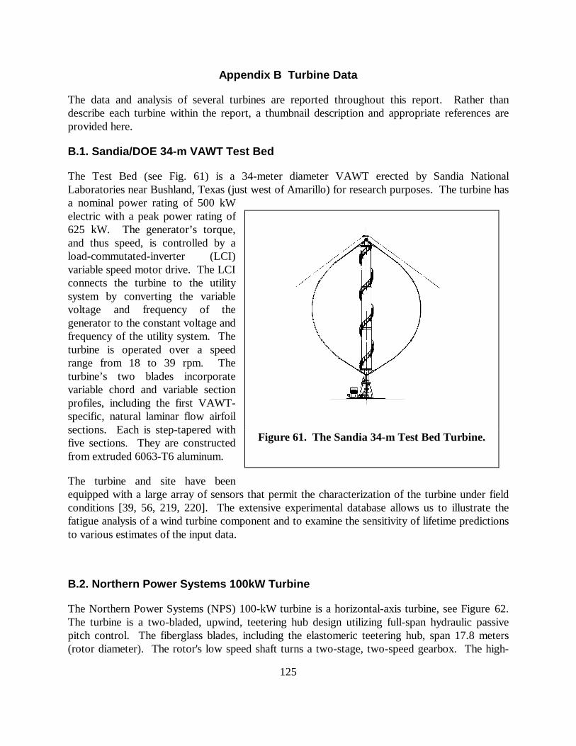
125

Appendix B Turbine Data

The data and analysis of several turbines are reported throughout this report. Rather thandescribe each turbine within the report, a thumbnail description and appropriate references areprovided here.

B.1. Sandia/DOE 34-m VAWT Test Bed

The Test Bed (see Fig. 61) is a 34-meter diameter VAWT erected by Sandia NationalLaboratories near Bushland, Texas (just west of Amarillo) for research purposes. The turbine hasa nominal power rating of 500 kWelectric with a peak power rating of625 kW. The generator’s torque,and thus speed, is controlled by aload-commutated-inverter (LCI)variable speed motor drive. The LCIconnects the turbine to the utilitysystem by converting the variablevoltage and frequency of thegenerator to the constant voltage andfrequency of the utility system. Theturbine is operated over a speedrange from 18 to 39 rpm. Theturbine’s two blades incorporatevariable chord and variable sectionprofiles, including the first VAWT-specific, natural laminar flow airfoilsections. Each is step-tapered withfive sections. They are constructedfrom extruded 6063-T6 aluminum.

The turbine and site have beenequipped with a large array of sensors that permit the characterization of the turbine under fieldconditions [39, 56, 219, 220]. The extensive experimental database allows us to illustrate thefatigue analysis of a wind turbine component and to examine the sensitivity of lifetime predictionsto various estimates of the input data.

B.2. Northern Power Systems 100kW Turbine

The Northern Power Systems (NPS) 100-kW turbine is a horizontal-axis turbine, see Figure 62.The turbine is a two-bladed, upwind, teetering hub design utilizing full-span hydraulic passivepitch control. The fiberglass blades, including the elastomeric teetering hub, span 17.8 meters(rotor diameter). The rotor's low speed shaft turns a two-stage, two-speed gearbox. The high-

Figure 61. The Sandia 34-m Test Bed Turbine.

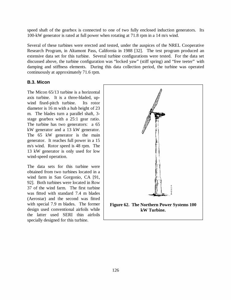
126

speed shaft of the gearbox is connected to one of two fully enclosed induction generators. Its100-kW generator is rated at full power when rotating at 71.8 rpm in a 14 m/s wind.

Several of these turbines were erected and tested, under the auspices of the NREL CooperativeResearch Program, in Altamont Pass, California in 1988 [32]. The test program produced anextensive data set for this turbine. Several turbine configurations were tested. For the data setdiscussed above, the turbine configuration was “locked yaw” (stiff spring) and “free teeter” withdamping and stiffness elements. During this data collection period, the turbine was operatedcontinuously at approximately 71.6 rpm.

B.3. Micon

The Micon 65/13 turbine is a horizontalaxis turbine. It is a three-bladed, up-wind fixed-pitch turbine. Its rotordiameter is 16 m with a hub height of 23m. The blades turn a parallel shaft, 3-stage gearbox with a 25:1 gear ratio.The turbine has two generators: a 65kW generator and a 13 kW generator.The 65 kW generator is the maingenerator. It reaches full power in a 15m/s wind. Rotor speed is 48 rpm. The13 kW generator is only used for lowwind-speed operation.

The data sets for this turbine wereobtained from two turbines located in awind farm in San Gorgonio, CA [91,92]. Both turbines were located in Row37 of the wind farm. The first turbinewas fitted with standard 7.4 m blades(Aerostar) and the second was fittedwith special 7.9 m blades. The formerdesign used conventional airfoils whilethe latter used SERI thin airfoilsspecially designed for this turbine.

Figure 62. The Northern Power Systems 100kW Turbine.

127

DISTRIBUTION:

R. E. AkinsWashington & Lee UniversityP.O. Box 735Lexington, VA 24450

H. AshleyDept. of Aeronautics and Astronautics Mechanical Engr.Stanford UniversityStanford, CA 94305

B. BellZond Energy Systems, Inc.13681 Chantico Rd.Tehachapi, CA 93561

K. BergeyUniversity of OklahomaAero Engineering DepartmentNorman, OK 73069

G. BirNREL/NWTC1617 Cole BoulevardGolden, CO 80401

M. BuhlNREL/NWTC1617 Cole BoulevardGolden, CO 80401

C. P. ButterfieldNREL/NWTC1617 Cole BoulevardGolden, CO 80401

G. BywatersNorthern Power Technology Co.Box 999Waitsfield, VT 05673

J. CadoganOffice of Photovoltaic & Wind Technologies, EE-11U.S. Dept. of Energy1000 Independence Avenue, SWWashington, DC 20585

D. CairnsMontana State UniversityDept. of Mechanical & Industrial Engr.Roberts HallBoseman, MT 59717

Stan CalvertOffice of Photovoltaic & Wind Technologies, EE-11U.S. Dept. of Energy1000 Independence Avenue, SWWashington, DC 20585

P. CarlinNREL/NWTC1617 Cole BoulevardGolden, CO 80401

J. ChapmanOEM Development Corp.840 Summer St.Boston, MA 02127-1533

M.C. ChaneyPS EnterprisesBox 837Glastonbury, CT 06033

R.N. ClarkUSDAAgricultural Research ServiceP.O. Drawer 10Bushland, TX 79012

128

J. CohenPrinceton Economic Research1700 Rockville PikeSuite 550Rockville, MD 20852

C. ColemanNorthern Power Technology Co.Box 999Waitsfield, VT 05673

K. J. DeeringThe Wind Turbine Company515 116th Avenue NENo. 263Bellevue, WA 98004

A.J. Eggers, Jr.RANN, Inc.Suite 26744 San Antonio Rd.Palo Alto, CA 94303

D. M. EgglestonDME Engineering1605 W. Tennessee Ave.Midland, TX 79701-6083

E. EgglestonUSDAAgricultural Research ServiceP.O. Drawer 10Bushland, TX 79012

P. R. GoldmanActing Deputy DirectorOffice of Photovoltaic & Wind Technologies, EE-11U.S. Dept. of Energy1000 Independence Avenue, SWWashington, DC 20585

G. GregorekAeronautical & Astronautical Dept.Ohio State University2300 West Case RoadColumbus, OH 43220

C. HansenUniversity of UtahDepartment of Mechanical EngineeringSalt Lake City, UT 84112

L. HellingLibrarianNational Atomic MuseumAlbuquerque, NM 87185

S. HockWind Energy ProgramNREL/NWTC1617 Cole BoulevardGolden, CO 80401

W. E. Holley3731 Oak Brook CourtPleasanton, CA 94588

K. JacksonDynamic Design123 C StreetDavis, CA 95616

G. JamesMechanical Engineering DepartmentUniversity of Houston4800 CalhounHouston, TX 77204-4792

J. JohnsonNREL/NWTC1617 Cole BoulevardGolden, CO 80401

129

N. KelleyNREL/NWTC1617 Cole BoulevardGolden, CO 80401

D. LainoUniversity of UtahDept. of Mechanical Engineering50 S. Central Campus Dr., Rm 2202Salt Lake City, UT 84112

R. LynetteSpringtyme Co.212 Jamestown Beach LaneSequim, WA 98382

D. Malcolm Kamzin Technology Inc.425 Pontius Avenue NorthSuite 150Seattle, WA 98109

J. F. Mandell (5)Montana State University302 Cableigh HallBozeman, MT 59717

J.F. ManwellUniversity of MassachusettsRenewable Energy Research LaboratoryE Lab Bldg., Dept. of Mechanical Engr.Amherst, MA 01003

R. N. MeroneyDept. of Civil EngineeringColorado State UniversityFort Collins, CO 80521

P. MiglioreNREL/NWTC1617 Cole BoulevardGolden, CO 80401

A. MikhailZond Energy Systems, Inc.13681 Chantico Rd.Tehachapi, CA 93561

L. MilesThe Wind Turbine Company515 116th Ave., NESuite 263Bellevue, WA 98004

R. H. MonroeGougeon Brothers100 Patterson AvenueBay City, MI 48706

W. MusialNREL/NWTC1617 Cole BoulevardGolden, CO 80401

NWTC LibraryNREL/NWTC1617 Cole BoulevardGolden, CO 80401

V. NelsonDepartment of PhysicsWest Texas A&M UniversityWT Box 60248Canyon, TX 79016

G. NixNREL/NWTC1617 Cole BoulevardGolden, CO 80401

J. W. OlerMechanical Engineering Dept.Texas Tech UniversityP.O. Box 4289Lubbock, TX 79409

130

Tim OlsenTim Olsen Consulting1428 S. Humboldt St.Denver, CO 80210

D. OngDept. of Aeronautics & AstronauticsStanford University98D Escondido VillagePalo Alto, CA 94305

R. OsgoodNREL/NWTC1617 Cole BoulevardGolden, CO 80401

R. PooreKamzin Technology Inc.425 Pontius Avenue NorthSuite 150Seattle, WA 98109

R. G. RajagopalanAerospace Engineering DepartmentIowa State University404 Town Engineering Bldg.Ames, IA 50011

J. Richmond3368 Mountain Trail Ave.Newbury Park, CA 91320

M. RobinsonNREL/NWTC1617 Cole BoulevardGolden, CO 80401

D.D. SamborskyMontana State Universityc/o Dr. John Mandell302 Cableigh HallBozeman, MT 59717

W. SassSecond Wind Inc.366 Summer St.Somerville, MA 02144

L. SchienbeinCWT Power4006 S. Morain LoopKennewick, WA 99337

D. SimmsNREL/NWTC1617 Cole BoulevardGolden, CO 80401

K. StarcherAEIWest Texas A&M UniversityWT Box 60248Canyon, TX 79016

F. S. StoddardP.O. Box 1373Amherst, MA 01004

R. W. ThresherNREL/NWTC1617 Cole BoulevardGolden, CO 80401

S. TsaiStanford UniversityDept. of Aeronautics and AstronauticsDurand Bldg.Stanford, CA 94305-4035

W. A. VachonW. A. Vachon & AssociatesP.O. Box 149Manchester, MA 01944

131

B. VickUSDA, Agricultural Research ServiceP.O. Drawer 10Bushland, TX 79012

J. WestergaardBoreal Enterprises5902 Seward Park Ave., SouthSeattle, WA 98118

R. E. WilsonMechanical Engineering Dept.Oregon State UniversityCorvallis, OR 97331

S. R. WintersteinCivil Engineering DepartmentStanford UniversityStanford, CA 94305

B. WolffRenewable Energy Program ManagerConservation and Renewable Energy System6918 NE Fourth Plain BoulevardSuite BVancouver, WA 98661

R. ZadoksUniversity of Texas at El Paso500 W. University Ave.Mechanical & Industrial Engr.El Paso, TX 79968-0521

M. ZuteckMDZ Consulting931 Grove StreetKemah, TX 77565

M. AndersonRenewable Energy Systems, Ltd.Beaufort House23 Grovesnor RoadSt. Albans, AL1 3AWUK

M. P. AnsellSchool of Material ScienceUniversity of BathClaverton DownBath BA2 7AYAvonENGLAND

P. W. BachNetherlands Energy Research Foundation,ECNP.O. Box 1NL-1755 ZG PettenTHE NETHERLANDS

J. BeurskensProgramme Manager for Renewable EnergiesNetherlands Energy Research Foundation,ECNP.O. Box 11755 ZG Petten (NH)THE NETHERLANDS

B. BulderNetherlands Energy Research Foundation,ECNP.O. Box 1NL-1755 ZG PettenTHE NETHERLANDS

D.R.V. van DelftDelft University of TechnologyStevin LabPO Box 5048260094 DelftTHE NETHERLANDS

132

J. B. DragtInstitute for Wind EnergyFaculty of Civil EngineeringDelft University of TechnologyStevinweg 12628 CN DelftTHE NETHERLANDS

R. A. GalbraithDept. of Aerospace EngineeringJames Watt BuildingUniversity of GlasgowGlasgow G12 8QGSCOTLAND

A. D. GarradGarrad Hassan9-11 Saint Stephen StreetBristol BS1 1EEENGLAND

P. JooseDelft University of TechnologyStevin LabPO Box 5048260094 DelftTHE NETHERLANDS

C. KenscheDLR –Institute of Structures and DesignGerman Aerosoace Research EstablishmentPfaffenwaldring 38-4070569 StuttgartGERMANY

D. I. PageEnergy Technology Support UnitB 156.7 Harwell LaboratoryOxfordshire, OX11 ORAENGLAND

T. F. PedersenRiso National LaboratoryPostbox 49DK-4000 RoskildeDENMARK

M. PedersenTechnical University of DenmarkFluid Mechanics Dept.Building 404Lundtoftevej 100DK 2800 LyngbyDENMARK

H. PetersenRiso National LaboratoryPostbox 49DK-4000 RoskildeDENMARK

P. H. MadsenRiso National LaboratoryPostbox 49DK-4000 RoskildeDENMARK

M. G. Real, PresidentAlpha Real AgFeldeggstrasse 89CH 8008 ZurichSWITZERLAND

D. SharpeDept. of Aeronautical EngineeringQueen Mary CollegeMile End RoadLondon, E1 4NSENGLAND

133

D. TaylorAlternative Energy GroupWalton HallOpen UniversityMilton Keynes MK7 6AAENGLAND

O. de VriesNational Aerospace LaboratoryAnthony Fokkerweg 2Amsterdam 1017THE NETHERLANDS

MS 0437 K. E. Metzinger, 09117MS 0437 E. D. Reedy, 09117MS 0439 C. R. Dohrmann, 09234MS 0439 D. W. Lobitz, 09234MS 0439 D. R. Martinez, 09234MS 0443 J. G. Arguello, 09117MS 0443 H. S. Morgan, 09117MS 0555 B. Hansche, 09133MS 0557 T. J. Baca, 09119MS 0557 T. G. Carne, 09119MS 0557 J. P. Lauffer, 09119MS 0557 T. W. Simmermacher, 09119MS 0615 J. H. Gieske, 09133MS 0708 H. M. Dodd, 06214 (50)MS 0708 T. D. Ashwill, 06214MS 0708 D. E. Berg, 06214MS 0708 P. L. Jones, 06214MS 0708 D. L. Laird, 06214MS 0708 M. A. Rumsey, 06214MS 0708 H. J. Sutherland, 06214MS 0708 P. S. Veers, 06214MS 0708 J. R. Zayas, 06214MS 0836 G. F. Homicz, 09116MS 0836 J. H. Strickland, 09116MS 0836 W. P. Wolfe, 09116MS 0619 Review & Approval Desk, 00111

For DOE/OSTIMS 0899 Technical Library, 04916 (2)MS 9018 Central Technical Files, 08940-2

Fatigue Analysis of Wind Turbines * -9, “f~ a, ,. *,. · led the wind turbine community to...

Documents

Transcript of Fatigue Analysis of Wind Turbines * -9, “f~ a, ,. *,. · led the wind turbine community to...