Fatigue analysis - local geometry optimization1251131/FULLTEXT01.pdf · UmeåUniversity July9,2018...

Umeå University July 9, 2018

Fatigue analysis - local geometry optimization

Anna Lundkvist ([email protected])

July 9, 2018

Abstract

The cause of fatigue failure is repeated loads, that cause cracks to appear andgrow even if the loads are far below the static load that would make a structure fail.High-cycle fatigue, which this project will focus on, is characterized by linear elasticstress and only fails after a large amount of loading cycles. While fatigue is the mostcommon cause of failure in structures, it is not feasible to calculate fatigue damageanalytically. The aim of this project was to develop, implement and test a workflowthat unifies the wide range of physical scales and transient features that are relevantto fatigue analysis of complex dynamic machinery. The workflow should take bothsystem-level and local aspects into account. The goal was to address both the globaland local while still keeping practical feasibility and simulation performance in mind.The resulting unified fatigue analysis method was then used on several test casesand illustrated from a local geometry optimization perspective.

The workflow contains the following steps: First the model is to be simulatedin order to get the load history. Then the finite element method (FEM) is usedto make a submodel of the component that is to be analyzed. The submodel issubjected to forces and moments, and then the stress is extracted from the areas ofinterest in the model. Thus, a linear relation for the stress can be calculated. Thestress history is calculated by putting the load history into the stress relation. Usingestablished fatigue analysis methods like rainflow counting and the Palmgren-Minerrule the fatigue life is then calculated.

This project only had its focus on the FEM submodel part of the fatigue work-flow. The geometry of the submodel should then be able to be optimized for thelongest fatigue life.

The workflow was tested on several test cases. The first one was a simple upside-down T-shaped component that was made by welding the parts together. The samecomponent but with no weld, as if it had been moulded, was the next case. Thefinal case was a component from the base of a crane. Two things were analyzed onthis case. The first was the fatigue life around a hole in which a shaft was welded.The other was optimizing to find the best position for a hook to be welded onto thesurface on the component.

Advisor at Algoryx: Peter [email protected]

Examinator: Martin [email protected]

Master’s Thesis in Engineering Physics

mailto:[email protected]



Anna Lundkvist ([email protected])Fatigue analysis - local geometry optimization

July 9, 2018

Contents

1 Introduction 3

2 Theory 42.1 Stress . . . . . . . . . . . . . . . . . . . . . . . . . . . . . . . . . . . . . . 4

2.1.1 Saint-Venant’s principle . . . . . . . . . . . . . . . . . . . . . . . . 42.2 Fatigue . . . . . . . . . . . . . . . . . . . . . . . . . . . . . . . . . . . . . 42.3 Current way of fatigue analysis . . . . . . . . . . . . . . . . . . . . . . . . 4

3 Fatigue Analysis Building Blocks 63.1 Stress amplitude and mean stress . . . . . . . . . . . . . . . . . . . . . . . 63.2 The S-N curve and the Basquin relation . . . . . . . . . . . . . . . . . . . 63.3 Palmgren-Miner rule . . . . . . . . . . . . . . . . . . . . . . . . . . . . . . 73.4 Rainflow counting . . . . . . . . . . . . . . . . . . . . . . . . . . . . . . . . 73.5 The hot spot method . . . . . . . . . . . . . . . . . . . . . . . . . . . . . . 8

4 Tools 94.1 Code_Aster . . . . . . . . . . . . . . . . . . . . . . . . . . . . . . . . . . . 94.2 WAFO . . . . . . . . . . . . . . . . . . . . . . . . . . . . . . . . . . . . . . 94.3 SpaceClaim Algoryx Momentum . . . . . . . . . . . . . . . . . . . . . . . 9

5 Method of unified fatigue analysis 105.1 Overview . . . . . . . . . . . . . . . . . . . . . . . . . . . . . . . . . . . . 105.2 Assumptions . . . . . . . . . . . . . . . . . . . . . . . . . . . . . . . . . . 115.3 Loads from dynamic system level simulation . . . . . . . . . . . . . . . . . 115.4 From loads to stress . . . . . . . . . . . . . . . . . . . . . . . . . . . . . . 12

5.4.1 The locked interface . . . . . . . . . . . . . . . . . . . . . . . . . . 135.5 From stress to weld model . . . . . . . . . . . . . . . . . . . . . . . . . . . 135.6 From weld model to rainflow counting . . . . . . . . . . . . . . . . . . . . 135.7 From rainflow counting to S-N curve . . . . . . . . . . . . . . . . . . . . . 145.8 From S-N curve to Miner-Palmgren rule . . . . . . . . . . . . . . . . . . . 14

6 Test cases 156.1 Case 1 . . . . . . . . . . . . . . . . . . . . . . . . . . . . . . . . . . . . . . 156.2 Case 1.5 . . . . . . . . . . . . . . . . . . . . . . . . . . . . . . . . . . . . . 166.3 Case 2 . . . . . . . . . . . . . . . . . . . . . . . . . . . . . . . . . . . . . . 17

7 Results 197.1 Case 1 . . . . . . . . . . . . . . . . . . . . . . . . . . . . . . . . . . . . . . 197.2 Case 1.5 . . . . . . . . . . . . . . . . . . . . . . . . . . . . . . . . . . . . . 197.3 Case 2 . . . . . . . . . . . . . . . . . . . . . . . . . . . . . . . . . . . . . . 20

1



July 9, 2018

8 Discussion 238.1 Case 1 . . . . . . . . . . . . . . . . . . . . . . . . . . . . . . . . . . . . . . 248.2 Case 1.5 . . . . . . . . . . . . . . . . . . . . . . . . . . . . . . . . . . . . . 248.3 Case 2 . . . . . . . . . . . . . . . . . . . . . . . . . . . . . . . . . . . . . . 25

9 Conclusion 26

10 References 27

A Appendix 28

B Appendix 30

2



July 9, 2018

1 Introduction

Fatigue is the most common cause of failure in mechanical structures. A structure maybreak when subjected to a repeated load far below what it would be able to bear in thecase of a static load. When designing a structure, it is often not possible to make it sothat it will never break from fatigue. Instead the designers aim to construct the structureso that it will not break during a sufficient long time, called its design life[1].

Unfortunately, there is no analytical way of calculating fatigue. Many assumptionshave to be made, and small differences in the material and in the surface affect the lifetime. The stress that is caused by the load that the structure is subjected to causesdamage, but that stress depends on the geometry of the component as well as residualstresses from welds or other things from its construction. The loading that the structureis subjected to may also not be exactly what it is designed against. For example, windsmay cause a crane stress. The use not being what the designer intended will also changethe life time. Corrosion is another thing that will make a component more susceptibleto fatigue failure.

When designing against fatigue, the use of standardized calculation procedures iscommon[1]. In order to get more accurate calculations, it is important that the load thatthe structure is subjected is as accurate as possible.

The problem with getting a good fatigue analysis today is that engineers hardly everare able to simulate the mechanical system in a way that gives the loadings with highresolution at the local level. Instead they have to rely on loading cases that are notnecessarily representative for the loads the structure will be subjected to in use. Butthey have no general work sequence they can get load history for. Even if they try touse conservative values that are supposed to be an high estimate of the damage it is stillpossible that they are too low.

The aim of this project is to create a workflow to calculate fatigue, and then optimizewith respect to local geometry. The workflow should be a procedure to use for componentswhere the user will check areas that they think are likely to break due to fatigue. Thenthe point with the shortest life time will be found.

On the construct that one wishes to do a fatigue analysis on, the part that should bemost susceptible to fatigue should be chosen. A submodel of that part will be made inorder to use the finite element method (FEM) to calculate the stress when the sub modelis subjected to unit forces. Then a linear relation will be calculated between the load andthe stress. By simulating the construct, the load history can be produced and the stresshistory is then calculated with the linear stress relation. At that point established fatigueanalysis methods can be used. That way, the stress that the component is subjected towill be more realistic compared when using loading cases, which will lead to more accurateresults.

This project will only focus on the FEM calculations and the stress model, as well asthe local geometry.

3



July 9, 2018

2 Theory

2.1 Stress

Stress is the force per area. If the stress is in the direction of the surface normal it iscalled normal stress. Stress that acts in the surface’s tangent plane is called skew stress.

The stress components at a point in Carthesian coordinates is

σij =

σxx σxy σxzσxy σyy σyzσxz σyz σzz

. (1)

The diagonal components are the normal stresses, and the non-diagonal are the skewstresses. Since every point is in equilibrium there is no net torque, and σij = σji[2].

2.1.1 Saint-Venant’s principle

Saint-Venant’s principle says that if a boundary condition is changed to a staticallyequivalent one the only difference is locally. Farther away from the boundary the solutionshould be approximately the same in the static case as it is in the original one. Twostatically equivalent loads should cause the same stress sufficiently far away from theloads. What constitutes as sufficiently far is not specified, but depends on the case.[3]

2.2 Fatigue

Fatigue is the failure caused by cyclic loads. A repeated load can cause failure even if it isfar below the static load that the structure can bear. Fatigue tests are carried out to findfatigue properties of materials and structures. Data for many materials and structureshave been published.

Fatigue is divided into two areas, high-cycle fatigue (HCF) and low-cycle fatigue(LCF). Low-cycle fatigue happens when there is high stress amplitudes or stress con-centrations and much plastic deformation occurs. The fatigue life is then considerableshorter. HCF does not have as dramatic plastic deformation, and the fatigue life is thenlonger[4]. This project will not consider LCF, and will instead focus on HCF.

Stress concentrations happens at the surface because of inhomogeneous stress distri-bution due to geometric factors. Therefore crack initiation happens at the surface of amaterial. The surface of a structure will thus affect its fatigue life[1].

Fatigue life is the number of cycles to failure. Under a certain stress amplitude,a specimen may never fail, no matter how many cycles it is subjected to. This stressamplitude is called the fatigue limit. However, damage to the surface, such as corrosion,will lower this limit, so it cannot be relied on. Some metals and metals alloys do nothave a fatigue limit[4].

2.3 Current way of fatigue analysis

The usual way to do a high-cycle fatigue analysis currently is shown in table 1.

4



July 9, 2018

Table 1 – An overview of a usual fatigue analysis workflow[5].

Step1 Find category that most closely corresponds to the detail of

the case2 Find loading case that corresponds most closely to the real

loading3 Use factors to account for dynamic and other effects4 Calculate fatigue life using the given values with a S-N curve

5



July 9, 2018

3 Fatigue Analysis Building Blocks

The building blocks in the fatigue analysis are the following

• σm

• σa

• S-N curve

• Miner-Palmgren rule

• Rainflow counting

• Weld model

• Loads from a dynamic, system level simulation

• Converting the loads to stress

These building blocks will be explained below.

3.1 Stress amplitude and mean stress

The stress amplitude, σa, is defined as half the stress range ∆σ:

σa =σmax − σmin

2=

∆σ

2. (2)

The mean stress is defined as [4]

σm =σmax + σmin

2. (3)

3.2 The S-N curve and the Basquin relation

A Wöhler curve, or S-N curve is obtained by doing fatigue tests at different stress levels.Plotting the stress amplitude σa versus the fatigue life Nf on a logarithmic scale gives alinear relation for a large range of Nf . This linear relation is called the Basquin relationand can be written as

σa = σ′f (2Nf )b, (4)

where σ′f is the fatigue strength coefficient and b is the Basquin exponent. The Basquinrelation is only valid when the mean stress, σm, is zero. But a modification was made byMorrow in 1968 to account for mean stress effects:

σa = (σ′f − σm)(2Nf )b. (5)

From this expression the fatigue life can be calculated[4].

6



July 9, 2018

3.3 Palmgren-Miner rule

The Palmgren-Miner rule is a simple model for fatigue damage accumulation. The fatiguedamage is calculated as

D =∑ ni

Nfi, (6)

where ni is number of cycles with the ith stress amplitude and Nfi is the fatigue life forthat stress amplitude. When D = 1 failure occurs.

The peak stress in a notch may be larger than the yield stress, the stress at whichthe material deforms plastically. If so plasticity will occur in the root of the notch andthat notch root plasticity can give compressive residual stress, which makes the damageof the following loading sequences milder. As such, the order of the loading sequencesdoes matter to fatigue damage, but is not taken in account by the Palmgren-Miner rule.

According to the Palmgren-Miner rule, the stress below the fatigue limit is non-damaging, since Nfi is infinite, and as such ni/Nfi = 0. But while stress amplitudesbelow the fatigue limit cannot create a growing microcrack under constant loading, if thespecimen has already been subjected to stress over the fatigue limit, the crack can growunder this stress.

The Palmgren-Miner rule was created to calculate the damage of loading with varyingamplitude, but does not have a physical basis to it. Fatigue damage is dependent on manyvariables, and cannot be described accurately with a single parameter. But despite itsweaknesses, the Palmgren-Miner rule has been found to work reasonably well and it iswidely used when calculating fatigue[1].

3.4 Rainflow counting

In order to analyze variable amplitude fatigue, cycle counting methods can be usedto turn the stress history into simple stress reversals. That way, the data obtainedfrom constant amplitude fatigue can be used to analyze the stress history. The rainflowcounting method is an example of a cycle counting method.

The idea of rainflow counting is to take the stress history and turn it 90° with thestart of time at the top. Imagine that stress history as a pagoda roof, with rain runningdown it. Start at a valley and let the water flow downwards. If the next valley is deeper,stop at the peak. Otherwise continue down to the next valley. When a rainflow stops,start a new one from the valley below the one where the last rainflow started. If a waterflow encounters another from above, it stops. Go through all valleys in that manner.The same is done for the peaks. That way, all the stress history should be countedin the rainflow. Then half-cycles are counted, and if the stress ranges and mean stressmatch, they are put together to whole cycles[4]. Finding the amplitude and mean ofthese cycles is easily done by checking the value the cycle starts and where it ends. Thenall information that is needed to use the Palmgren-Miner rule is present.

In fig. 1 an example of rainflow counting is shown for a simple stress history.

7



July 9, 2018

Figure 1 – An example of rainflow counting done on a simple stress history.[6]

There are of course algorithms that can perform rainflow counting on the stress historydata.

3.5 The hot spot method

A hot spot is a critical point where a crack is assumed to grow. In a welded structure,the hot spot is at the weld toe. The hot spot stress is defined as the geometrical stressat the hot spot. At the hot spot, there is usually an non-linear stress distribution causedby the geometry of the weld. This area is estimated to be within a radius of 0.4t and0.3t, where t is thickness of the structure. The geometrical stress does not include thenon-linear stress peak, by definition. Getting the geometrical stress in the hot spot canbe done by extrapolation. The equation for quadratic extrapolation is

σhs = 2.52σ0.4t − 2.24σ0.9t + 0.72σ1.4t, (7)

where σx is the surface stress x mm away from the weld toe[7].

8



July 9, 2018

4 Tools

The tools used to do the fatigue analysis will be presented here.

4.1 Code_Aster

Code_Aster is a free FEM software, made by EDF R&D. It is available on Unix andLinux, and the command language is in Python[8].

Salome-Meca is a platform that can be used with Code_Aster. Using Salome-Meca’sGeometry module, the geometry can be defined either through tools of the platform orby importing a file describing it. In the Mesh module, the mesh can be computed, using anumber of algorithms. Parameters such as maximum and minimum size of elements canbe change in order to get a mesh suitable to one’s needs. It is also possible to set localsizes on areas and edges of the geometry. Groups of nodes, or faces on the mesh, can bedefined from the geometry, or by the user selecting them. These groups are needed toextract values or set a force on them.

Eficas Command File Editor and Syntax Analyser can be used to generate commandfiles for Code_Aster with correct syntax. Writing other Python code, for example whenpost-processing, must be done outside Eficas[8].

In the command file, the model for the case is chosen. All cases in this project use the3D model. However, moments cannot be added directly to 3D models in Code_Aster.To get moment onto the 3D model it can be added to a free node that one connects tothe group of nodes on the face on the 3D model.

In the Aster module study cases are made, by choosing a command file and a mesh.In the Aster module the interface ASTK can be run. From ASTK it is possible to usethe data from a previous run as the base for a new one, which makes it convenient touse for post-processing in a separate run. This is useful when the original solution takesa long time.

The results can be inspected in the module ParaViS.

4.2 WAFO

WAFO stands for Wave Analysis for Fatigue and Oceanography, and it is a Pythonpackage for statistical analysis and simulation of random waves and loads. It containsfunctions for rainflow counting[9].

The version of NumPy that WAFO uses is a newer version than the one Code_Aster2016 uses. In order to get WAFO work in a script run by Code_Aster 2016 the versionof NumPy has to be replaced by the version used by WAFO.

4.3 SpaceClaim Algoryx Momentum

SpaceClaim is a 3D modeling CAD software. It is available on Windows. It has the add-on Algoryx Momentum, a multibody dynamics tool. With Momentum, it is possible tosimulate the models in SpaceClaim. Momentum will not be directly used in this project,but data from Momentum simulations will be used.

9



July 9, 2018

5 Method of unified fatigue analysis

Here the way of unifying the fatigue analysis building blocks into a workflow will bepresented. The order is first presented in table 2 and after an overview the path betweenthe building blocks will then be explained.

Table 2 – The order of the fatigue analysis building blocks.

Loads from dynamic system level simulation|

Converting the loads to stress|

Weld model|

Rainflow counting|

σa, σm|

S-N curve|

Palmgren-Miner rule

5.1 Overview

The fatigue analysis workflow is summarized in table 3. Step 2 through 5 are the newparts in this workflow, while the steps after them are general fatigue analysis steps thatare also used elsewhere.

In order to use this workflow some things are necessary. First, a way to use multibodydynamics, to simulate a moving mechanical systems. Second, a FEM tool which letsthe user subject the model to many different loading cases. Third, a rainflow countingalgorithm. In appendix B the code for the process from step 5 and below is available forthe same case.

10



July 9, 2018

Table 3 – An overview of the fatigue analysis workflow.

Step1 Simulate model for load history2 Make sub model with FEM3 Lock one interface, subject others to unit forces and moments4 Calculate linear relation between stress and load5 Put load history in stress relation to get stress history6 Use rainflow counting to get stress amplitude, mean stress

and number of cycles7 Find properties σ′f and b8 Use the Basquin relation to calculate the fatigue life of the

cycles9 Calculate damage from number of cycles and their respective

fatigue life with Palmgren-Miner rule10 Calculate total fatigue life

5.2 Assumptions

There are several assumptions made in the calculation of the fatigue life.It is assumed that the sub model is large enough for Saint-Venant’s principle to be in

effect, that the point that is analyzed is far enough from the boundary that the change inthe boundary condition will not matter. However it is also assumed that the sub modelis small enough that it can be looked at as a static model.

The fatigue is assumed to be high-cycle fatigue.The The load-stress relation is assumed to be linear.Both the rainflow counting and the Palmgren-Miner rule assumes that the order of

the stress does not matter for the fatigue life.Overall it is assumed that the established fatigue methods as the Palmgren-Miner

rule, Rainflow counting, the S-N curve and so on give correct results.The superposition principle is used, which is possible since the stress is linear.

5.3 Loads from dynamic system level simulation

First a model is made in Algoryx Momentum to simulate the appropriate loadings. Fromthis simulation, the load history is extracted.

11



July 9, 2018

5.4 From loads to stress

The method to get the stress from the load was the most important step in this project,as it is the new one that created in order for the workflow to work, while the othersteps are established methods. The approach was devised by Peter Norlindh at AlgoryxSimulation AB.

The idea is that when analyzing high-cycle fatigue go from a dynamic system toa quasi-static one. Using a submodel of a size such that the dynamic effects can beneglected, as well as Saint-Venant’s principle and the superposition principle, arbitrarycombinations of loads can be applied on an arbitrary number of mechanical interfaces inorder to calculate the stress resulting from those loads. In practice, this means convertingthe load history to stress by making a submodel with FEM and calculating a linearrelation between the stress and the load.

By taking a submodel of the original model and then making a linear relation of thestress to put the load history into, the size of the calculations that have to be made andthe data that has to be handled are dramatically reduced. Extracting the stress historydirectly from a complete model would be a much too complicated task, but by usinga submodel the problem lessens considerably. It will still be a too long and complexprocedure to project the load history onto the submodel to get the stress history, andeven that may not even be possible considering that the load history can be very longand complicated. It is a very quick process to instead put the load history into the linearrelation to get the stress history. This means that the method makes it possible to applyan arbitrary combination of loads and get the stress tensor corresponding to them almostinstantaneously. This is what makes the fatigue analysis possible in practice.

This process is as follows: In Code_Aster, a submodel of the original model is made.This is a static model, unlike the one in Algoryx Momentum. The places where thesubmodel connects with the rest of the model are called mechanical interfaces and arewhere the submodel is subjected to the loads. One of the mechanical interfaces are lockedin all degrees of freedom. The other interfaces are subjected to unit forces, one in eachdirection, x, y and z, as well as all three moments, mx, my and mz. The moments arearound the x-, y-, and z-axis, respectively. These loads are applied evenly over the area ofthe mechanical interface. The loads are applied separately. Then the stress componentsresulting from the different loads are extracted from the places on the component wherethe stress should be concentrated, like notches or welds. From this data, a linear relationbetween the loads and the stress is calculated. That linear relation is:

σij = LklCklij (8)

where k stands for the mechanical interfaces and l = 1, ..., 6 and correspond to the loadsfx, fy, fz, mx, my and mz, in that order. The number of mechanical interfaces dependson the case. The equation describes the stress for one point (node) on the sub model.The first 6k rows thus correspond to the first node, with the first six rows correspondingto the first interface. The first row is then the stress components caused by the unit forcefx the first interface is subjected to, and the the seventh is the stress components caused

12



July 9, 2018

by fx on the second interface.The load history is formatted so that each mechanical interface has its own file with

loads. In it, each row is a time step, and the columns are the load components. Byputting the load history in the linear relation corresponding to the extrapolation points,the stress is calculated. The stress is summed up in its components. For example,σxx on one node with loads from different interfaces are summed up, but the six stresscomponents are separate. If there are n mechanical interfaces then the normal stress inthe x direction is

σxx =n∑

k=1

6∑l=1

LklCklxx. (9)

The Code Aster script writes a file with the constants for the linear relation betweenthe load and the stress. In appendix A the code for the process of calculating the stressrelation and saving the constants can be found. This is for the test case that is describedin section 6.3.

5.4.1 The locked interface

When calculating the linear relation of the load and the stress, one interface is held stillby constraints in all degrees of freedom. The other interfaces are subjected to unit forcesand moments in all directions, one at a time.

It is not necessary to subject the locked interface to loads in order to get the stressesthose loads would incur. The reason for this is that when the other interfaces are sub-jected to all possible loads, there will be an opposing force on the locked interface thatholds it in place. Therefore, those loads will also affect the locked interface. The opposingforce holding the interface in place will also cause stress. The stress that would happenif the locked interface was being affected directly by a load, with another interface beinglocked in its stead, will already have appeared, so there is no need to have separate casesto cover those loads.

5.5 From stress to weld model

The weld model used is the hot spot method. The extrapolation points used by thehot spot method are known, since the geometry of the component is known. The nodesclosest to the points can then be found.

From the stress components the hot spot stress is extrapolated, using eq. 7. If thecomponent does not have a weld, it is not necessary to use the hot spot method. Thenthe stress history on the nodes is used directly.

5.6 From weld model to rainflow counting

Using rainflow counting on the stress history from the hot spot method gives the numberof cycles, stress amplitude, σa, and mean stress, σm. In fig. 2 the data that one gets

13



July 9, 2018

from a rainflow counting is shown in a histogram. The rainflow counting is done for eachstress component, instead of putting all the stress components into one stress variable.

Figure 2 – The data that is gotten from a rainflow counting shown in a histogram[10].

Below is an example of using WAFO on the stress components.

f o r i in range ( no_stress_comp ) :t_sigma = np . column_stack ( ( t , sigma [ : , i ] ) )t s1 = wo . mat2t imeser i e s ( t_sigma )t ry :

s ig_tp = ts1 . turn ing_points (h=−1, wavetype='astm ' )except ValueError :

s ig_tp = Nonetry :

sig_cp = sig_tp . cycle_astm ( )except Att r ibuteError :

sig_cp = None

The sig_cp variable then contains the stress amplitude, the mean stress and thenumber of cycles.

5.7 From rainflow counting to S-N curve

The stress amplitude and mean stress is then used to calculate the fatigue life for therespective cycles, using the Basquin relation from the S-N curve.

5.8 From S-N curve to Miner-Palmgren rule

Finally, the Palmgren-Miner rule is used to calculate the total fatigue life of the compo-nent. The point which has the shortest fatigue life is saved, with the value of the fatiguelife.

14



July 9, 2018

6 Test cases

6.1 Case 1

The first case is a component shaped like an upside down T. The vertical part is weldedto the horizontal bottom part. In fig. 3 the component is shown, with the coordinatesystem. The lines on the components shows where the sub model is.

The component can only move horizontally and is subjected to a loading F (x) =5 · 106 sin(50πt) + 3 · 106 sin(37πt), where t is the time.

Figure 3 – The T-shaped component.

The sub model is shown in fig. 4. The top part is held still with all degrees of freedomlocked, while the left and right mechanical interfaces are subjected to unit forces andmoments in different directions.

Figure 4 – The sub model of the T shaped component.

The table 4 shows the measurements for the sub model.

15



July 9, 2018

Table 4 – The measurements of the sub model of the component.

Measurement [mm]L 29.0h 14.0t1 6.0t2 5.0w 5.0

Table 5 shows the material properties for component.

Table 5 – This table contains the material properties of the component.

Property Valueb -0.13σ′f 756 · 106

ν 0.29E 2.05 · 1011 Pa

Since the component is symmetric, it is only necessary to analyze one of the welds, onone of the sides of the component. As such, the left side has been chosen to be analyzed.Both weld toes of that weld will be analyzed, the vertical as well as the horizontal one,with the hot spot method. The welds will be analyzed at points over their whole lengthsand the ones with the shortest fatigue life will be found.

6.2 Case 1.5

This case is similar to case 1, but this component is not welded. Instead it has beenmoulded. The places where the welds where are now rounded, with radius r = 3 mm.Otherwise all is the same as in case 1. But since there is no weld to be modeled, thehot spot method will not be used to calculate the fatigue life. Instead the stress can becalculated directly in the area where the component is most likely to break. The submodel is shown in fig. 5.

16



July 9, 2018

Figure 5 – The sub model of the T-shaped component that was not welded.

Again, the model is symmetric, so only the left side will be analyzed.

6.3 Case 2

The second case is a model of a crane, taken from GrabCAD[11]. The grapple[12] andthe rotator[13] is from other files from GrabCAD and have been added to the crane.

The sub model was exported from Space Claim as a stp-file and imported intoCode_Aster. In fig. 6 crane and the sub model is shown.

(a) The complete crane. (b) The submodel of thecrane.

Figure 6 – The model and the submodel of the crane.

Table 6 shows the material properties for crane sub model. The work sequence is thecrane picking up a tree trunk and placing it into a box.

17



July 9, 2018

Table 6 – This table contains the material properties of the crane submodel.

Property Valueρ 7870 kg/m3

ν 0.29E 2.05· 1011 Pa

b -0.13σ′f 168 · 106

First the fatigue life around the upper hole was considered. In the hole a shaft iswelded. It is around the shaft that the crane arm moves, so the sub model is completelystatic. The hot spot method was used to consider the boundary around the hole.

But another analysis was also made on the crane component. The best placementwas found for a hook to be used to move the crane. By optimizing over a line on thesurface of the component, y = kz + m, going from p1 = [0.23452, 1.7447,−2.2979] top2 = [0.23452, 0.81952,−2.56391]. Thus, x was constant on the surface. On that linethe spot which had the longest fatigue life was found. That point should be the bestplacement for the hook, so that the stresses made by welding a hook in place woulddo as little damage as possible. The hook was not added to the geometry when theoptimization took place.

The two outer points of the hook were analyzed using the hot spot method, underthe assumption that the hook was 75 mm across. The shortest lifetime of the two pointswas saved. The placement which had the longest fatigue life on its shortest point wasfound as the optimal placement.

18



July 9, 2018

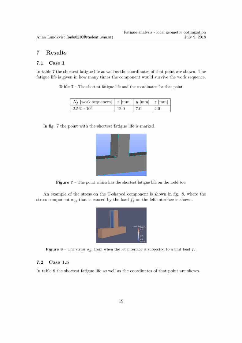
7 Results

7.1 Case 1

In table 7 the shortest fatigue life as well as the coordinates of that point are shown. Thefatigue life is given in how many times the component would survive the work sequence.

Table 7 – The shortest fatigue life and the coordinates for that point.

Nf [work sequences] x [mm] y [mm] z [mm]2.561 · 109 12.0 7.0 4.0

In fig. 7 the point with the shortest fatigue life is marked.

Figure 7 – The point which has the shortest fatigue life on the weld toe.

An example of the stress on the T-shaped component is shown in fig. 8, where thestress component σyz that is caused by the load fz on the left interface is shown.

Figure 8 – The stress σyz from when the let interface is subjected to a unit load fz.

7.2 Case 1.5

In table 8 the shortest fatigue life as well as the coordinates of that point are shown.

19



July 9, 2018


Nf [work sequences] x [mm] y [mm] z [mm]6.539 · 107 12.0 9.0 3.429

In fig. 9 the point with the shortest fatigue life is marked.

Figure 9 – The point with the shortest fatigue life.

An example of the stress on the component is shown in fig. 10, where the stresscomponent σxy that is caused by the load fx on the left interface is shown.

Figure 10 – The stress σxy from when the left interface is subjected to a unit load fz.

7.3 Case 2

The results of the fatigue analysis around the hole with both work sequences can foundin table 9. The work sequence where the crane is almost still is referred to loading case1. The other, in which a tree trunk is lifted, is called work sequence 2.


Nf [work sequences] x [m] y [m] z [m]4.107 · 103 0.23452 2.133874 -2.267016

In fig. 11, the component is shown with the failing point.

20



July 9, 2018

Figure 11 – The point with the shortest fatigue life around the hole.

Table 10 shows the optimal placement for the hook along the line, as well as thefatigue life for that placement.

Table 10 – The longest fatigue life and the coordinates for that point.

Nf [work sequences] x [m] y [m] z [m]1.304 · 108 0.23452 1.7447 -2.2979

In fig. 12 the point for the placement of the hook’s left corner is marked.

Figure 12 – The point where the hook’s left corner should be placed for the longestfatigue life.

An example of the stress on the component is shown in fig. 13, where the stresscomponent σyy that is caused by the load fx on the upper interface is shown.

21



July 9, 2018

Figure 13 – The stress σyy from when the upper interface is subjected to a unit load fz.

22



July 9, 2018

8 Discussion

The advantages of simulating the load history are obvious. It is possible to get the generalloadings the component will be subjected to, instead of just a loading case that may ormay not be representative of the general work sequence. Having a more realistic load willgive a much more accurate result when doing a fatigue analysis. In order to use the loadhistory from the simulation it is necessary to convert the load history to stress history,since it is impossible to get the stress directly from the simulation. There are two stepsto that process. First there is the submodel, and secondly there is the linear relation.By taking a submodel the problem is made smaller since the submodel is smaller as wellas much less complicated than the whole model as it is static. Even so, projecting theload history onto the submodel would be complicated and time-consuming consideringhow complicated the load history may be. The load history would need to be accurateto the real one, which can be very varied, and thus the simulation would need to go onfor a long time to give a long load history. Therefore the linear relation is calculated inorder to get a way to quickly convert the load history to stress. The relation also doesnot need to be calculated for the whole model. It is enough that it is done for the areaaround the weld toe, if there is a weld. This again reduces the amount of data that needsto be saved.

There are some known weaknesses of the methods used that could be considered:Palmgren-Miner is not based on a physical argument, but is a simplistic way to sum upthe fatigue damage. It is difficult to avoid using it when doing fatigue analysis, sincethere are no physics-based way of calculating damage. However, a new way of calculatingdamage is far outside the scope of this project, which is supposed to use already knownmethods.

Rather than using the fatigue limit, the Basquin relation is also used for stressesbelow the limit. This way, the damage from stresses that should be non-damaging aretaken into account, which is a good thing, since those stresses can cause damage if theycome after stresses that have already caused a microcrack. Since the order of the stressesare not taken into account it is better to assume the stresses below the fatigue limit causedamage. That way, the actual damage will not be above the estimate, and the resultshould be conservative.

In the test cases the weld is not modeled. Instead the place where the weld should beis smooth as if component were just in one piece from the beginning. Since the geometryis supposed to be taken into account with the hot spot method, the geometry shouldmatch the true one as much as possible. So for a more accurate result, it may be a goodidea to model the weld.

A possible improvement would be to streamline the process so that the geometrycan be changed and the fatigue analysis for the change can run automatically, insteadof spending time on meshing and renaming node groups. Currently every change in thegeometry needs to be imported into Code_Aster and then meshed. Then mesh groupsneed to be defined in so that it is possible to subject the mechanical interfaces to loadsand extract data from interesting parts. This is inconvenient for optimization.

23



July 9, 2018

Someone who does not have much knowledge of fatigue will have a hard time usingthe work flow. The method needs an engineer who can find the areas which should beanalyzed. They need to first choose the right sub model, and then the right point on thesub model. The whole sub model would take far too long to check. This means that itis up to the engineer to have an understanding of where the weak points are, or to checksimilar constructs and where they usually fail. However, this is not much of a weakness.If someone is to work with analyzing fatigue, it is reasonable to expect that they havesuch an understanding.

It is possible to do an analysis on all the nodes of a larger area than what is donein the test cases. It is the calculation of the linear relation that takes time. Whencalculating the relation stress data from the nodes are extracted for all the different loadcases. But over a larger area this would take a lot of time so it would not be feasible toanalyze too large an area.

8.1 Case 1

In case 1, the component breaks in the weld toe on its vertical part. This is as expected,since the vertical part is slightly thinner than the horizontal one. The upper part isnot supported by anything, so the stress should be higher on its base than it is on thehorizontal part. However, the point where it fails is asymmetrical, which is unexpectedconsidering the component’s symmetric geometry and the even distribution of the loadon the interface. This might be due to nothing more than slight variations over the weldtoe.

There is some inaccuracies in the solution, since the nodes where the stress were takenfrom to extrapolate the hot spot stress is not exactly where the extrapolation points are.If the mesh is too coarse, then the closest node to the extrapolation point can be quitea distance away. Here the distance should not be large enough to affect the result much.In a real case, the best thing to do would be do make another version with a finer meshand compare the result to make sure the mesh is not affecting the results. However, sincethis is just a test case to try the method, it is not necessary.

The size of the sub model may also affect the results. The stresses from the lockedinterface are very high close to it, so if the sub model has been chosen too small, thenthe stresses from the locked interface may interfere. When the hot spot method is used,extra caution is needed to make sure the extrapolation points do not end up to close tothe locked interface. This is because of the high stresses that occurs when the componentis held in place.

8.2 Case 1.5

This is the only test case when the hot spot method is not used. Since no extrapolationpoints are needed, there is no error from not having the node slightly off where it shouldbe. But that does not mean that this case is more accurate than the first one. By takingthe hot spot stress, the hot spot method attempts to take the geometry in consideration.

24



July 9, 2018

The fatigue life is shorter for this case than it is in case 1. This seems counterintuitive,since a weld is supposed to be a weak point. The most probable reason for this resultis that the hot spot method uses the hot spot stress to estimate the geometric stress,and as such does not take into account the total stress. In case 1.5, no estimation of thestress behavior has been made. Instead the calculation is made directly after the stressin the points that have been deemed to be likely to fail.

Since the hot spot method is not used and no certain point need to be found toextrapolate from, the mesh is not especially fine. This can also be a reason why for thedifference in result for case 1 and case 1.5.

8.3 Case 2

If the results of the fatigue life of the placement of the hook is compared with the fatiguelife around the hole, it is obvious that it will break first around the hole. But it is moreinteresting to look at the cases separately to use the hook as an example on how to try tooptimize the geometry, rather than dismiss the placement because it will break anywayin another spot.

Optimizing the placement of the hook is done without adding the hook to the ge-ometry. Not having the geometry of the hook when calculating the stress may give aninaccurate result, especially since the hot spot method is supposed to take the geometryin consideration. However, the hook itself is not likely to have added much stress to thecomponent. The place where the stress on the surface without the hook is largest shouldalso be the place where the hook would do the most damage. The actual fatigue lifemay change, but it is likely not a large difference, unless one checks for when the craneis lifted with the hook.

The fatigue life is the only thing taken into account when optimizing the placementfor the hook. Where it is most practical to have the hook, and where it would be easiestto move the crane is not, but that would of course be needed when doing this for a realcase. It would not matter how long it would hold, if it would be impossible to use becauseof an impractical placement.

25



July 9, 2018

9 Conclusion

This fatigue analysis workflow has some rough edges to be filed off, but should give anrealistic stress history that gives a more accurate fatigue life than commonly used waysof calculating fatigue.

In order to use this workflow to optimize the geometry more work is needed since itis not a very streamlined procedure in the present. However, at the present it works andproduces reasonable results.

26



July 9, 2018

10 References

[1] Schijve, J., Fatigue of structures and materials, 2nd ed. Springer, 2009.

[2] Sundström, B., Handbok och formelsamling i hållfasthetslära, 2nd ed. Södertälje:Fingraf AB, 1999.

[3] Reddy, J. N., An introduction to continuum mechanics. Cambridge UniversityPress, 2008.

[4] Suresh, S., Fatigue of materials, 2nd ed. Cambridge University Press, 2004.

[5] European Committee for Standardization, Eurocode 3: Design of steel structures -part1-9: Fatigue, Brussels, Belgium, 2005.

[6] Irvine, T., Rainflow cycle counting in fatigue analysis, 2011-08-26. [Online]. Avail-able: https://pdfs.semanticscholar.org/e866/3ef9235a09845b0eb065531b036ee207c89b.pdf.

[7] Eriksson, Å. and Lignell, A.-M., Svetsutvärdering med fem. Industrilitteratur AB,2002.

[8] EDF R&D, Code_Aster - Analysis of Structures and Thermomechanics for Studies& Research, EDF, Clamart, France, 2000. [Online]. Available: https://www.code-aster.org/UPLOAD/DOC/Presentation/plaquette_aster_en.pdf.

[9] WAFO-group, WAFO - a matlab toolbox for analysis of random waves and loads- a tutorial, ISBN XXXX, Math. Stat., Center for Math. Sci., Lund Univ., Lund,Sweden, 2000. [Online]. Available: http://www.maths.lth.se/matstat/wafo.

[10] Nieslony, A., Grainflow counting algorithm, 2017-12-19. [Online]. Available: https://se.mathworks.com/matlabcentral/fileexchange/3026-rainflow-counting-algorithm?.

[11] Doxsyde, Guindaste - STEP/IGES, STL - 3D CAD model, 2017-12-14. [Online].Available: https://grabcad.com/library/guindaste.

[12] Per, Grapple - STL, STEP/IGES - 3D CAD model, 2017-12-14. [Online]. Available:https://grabcad.com/library/grapple.

[13] Marcelo, Rotator - STEP/IGES - 3D CAD model, 2017-12-14. [Online]. Available:https://grabcad.com/library/guindaste.

27


https://pdfs.semanticscholar.org/e866/3ef9235a09845b0eb065531b036ee207c89b.pdf

https://pdfs.semanticscholar.org/e866/3ef9235a09845b0eb065531b036ee207c89b.pdf

https://www.code-aster.org/UPLOAD/DOC/Presentation/plaquette_aster_en.pdf

https://www.code-aster.org/UPLOAD/DOC/Presentation/plaquette_aster_en.pdf

http://www.maths.lth.se/matstat/wafo

https://se.mathworks.com/matlabcentral/fileexchange/3026-rainflow-counting-algorithm?

https://se.mathworks.com/matlabcentral/fileexchange/3026-rainflow-counting-algorithm?

https://grabcad.com/library/guindaste

https://grabcad.com/library/grapple

https://grabcad.com/library/guindaste


July 9, 2018

A Appendix1 # Fatigue analysis on sub model of crane component2

3 DEBUT();4

5 import numpy as np6 import wafo.objects as wo7

8 # Initialize parameters9 no_load_cases = 12

10 resu = [None]*no_load_cases11 tab = [None]*no_load_cases12

13 # First left interface, all load cases, then right interface14 interface = ['h1','h1','h1','h1','h1','h1',15 'h2', 'h2', 'h2','h2', 'h2', 'h2']16 # The node which transfers momentum to 3D model (not used in cases fx, fy, fz)17 node = ['none', 'none', 'none', 'node1', 'node1', 'node1',18 'none', 'none', 'none', 'node2', 'node2', 'node2']19

20 # Read mesh file21 mesh0=LIRE_MAILLAGE(FORMAT='MED',);22 # Make mesh groups to stand alone nodes23 mesh=CREA_MAILLAGE(MAILLAGE=mesh0,24 CREA_POI1=(_F(NOM_GROUP_MA='node1',25 GROUP_NO='node1',),26 _F(NOM_GROUP_MA='node2',27 GROUP_NO='node2',),),);28

29 # Assign model30 model=AFFE_MODELE(MAILLAGE=mesh,31 AFFE=(_F(TOUT='OUI',32 PHENOMENE='MECANIQUE',33 MODELISATION='3D',),34 _F(GROUP_MA=('node1','node2',),35 PHENOMENE='MECANIQUE',36 MODELISATION='DIS_TR',),),);37

38 # Define material39 mat=DEFI_MATERIAU(ELAS=_F(E=6.895E+10,40 NU=0.33,41 RHO=2705.0,),);42

43 # Apply material44 ap_mat=AFFE_MATERIAU(MAILLAGE=mesh,45 AFFE=_F(GROUP_MA='Solid',46 MATER=mat,),);47

48 # Boundary condition49 bc=AFFE_CHAR_MECA(MODELE=model,50 DDL_IMPO=_F(GROUP_MA='bottom',51 DX=0.0,52 DY=0.0,53 DZ=0.0,),);54 # Loop over the load cases55 for i in range(no_load_cases):56

57 # Define boundary conditions and load for different load cases58 if i == 0 or i == 6:59 load=AFFE_CHAR_MECA(MODELE=model,

28



July 9, 2018

60 FORCE_FACE=_F(GROUP_MA=interface[i],61 FX=1.0,),);62 elif i == 1 or i == 7:63 load=AFFE_CHAR_MECA(MODELE=model,64 FORCE_FACE=_F(GROUP_MA=interface[i],65 FY=1.0,),);66 elif i == 2 or i == 8:67 load=AFFE_CHAR_MECA(MODELE=model,68 FORCE_FACE=_F(GROUP_MA=interface[i],69 FZ=1.0,),);70 elif i == 3 or i == 9:71 load=AFFE_CHAR_MECA(MODELE=model,72 LIAISON_SOLIDE=_F(GROUP_NO=(interface[i],node[i],),),73 FORCE_NODALE=_F(GROUP_NO=node[i],74 MX=1.0,),);75 elif i == 4 or i == 10:76 load=AFFE_CHAR_MECA(MODELE=model,77 LIAISON_SOLIDE=_F(GROUP_NO=(interface[i],node[i],),),78 FORCE_NODALE=_F(GROUP_NO=node[i],79 MY=1.0,),);80 elif i == 5 or i == 11:81 load=AFFE_CHAR_MECA(MODELE=model,82 LIAISON_SOLIDE=_F(GROUP_NO=(interface[i],node[i],),),83 FORCE_NODALE=_F(GROUP_NO=node[i],84 MZ=1.0,),);85

86 # Apply characteristics to the two nodes87 cara=AFFE_CARA_ELEM(MODELE=model,88 DISCRET=_F(CARA='K_TR_D_N',89 GROUP_MA=('node1','node2',),90 VALE=(0.1,0.1,0.1,0.1,0.1,0.1,),),);91

92 # Solve the problem93 resu[i]=MECA_STATIQUE(MODELE=model,94 CHAM_MATER=ap_mat,95 CARA_ELEM=cara,96 EXCIT=(_F(CHARGE=bc,),97 _F(CHARGE=load,),),);98

99 # Calculate stress100 resu[i]=CALC_CHAMP(reuse =resu[i],101 RESULTAT=resu[i],102 CONTRAINTE='SIGM_NOEU',103 FORCE='FORC_NODA',);104

105 # Write result to med file, in case you want to look at it in ParaViS106 IMPR_RESU(FORMAT='MED',107 RESU=_F(RESULTAT=resu[i],108 INFO_MAILLAGE='OUI',109 TOUT='OUI',110 GROUP_MA='Solid',),);111

112

113 # Destroy old parameters114 if i < no_load_cases-1:115 DETRUIRE(CONCEPT = _F (NOM = load,) ,INFO=1, );116 DETRUIRE(CONCEPT = _F (NOM = cara,) ,INFO=1, );117

118

119 FIN();

29



July 9, 2018

B Appendix1 # Fatigue analysis on submodel of crane component2 #3 # Reads the load history from files crane_load1_moving.txt, crane_load2_moving.txt4 # from the two side mechanical interfaces and the time from crane_times_moving.txt.5 #6 # Calculates a linear relation between the load and the stress and saves the7 # constants for the boundary around the upper hole as well as the coordinates8 # for the nodes9 #

10 # Uses the hot spot method to calculate fatigue life at weld on the hole's boundary.11 # Writes fatigue life to a file, results.txt.12

13

14 # Function to extract stress components for nodes from table15 def extractStress(table):16 table0 = table.EXTR_TABLE()17 pytab = table0.values()18 # Extract stress coefficients19 sxx=pytab['SIXX']20 syy=pytab['SIYY']21 szz=pytab['SIZZ']22 sxy=pytab['SIXY']23 sxz=pytab['SIXZ']24 syz=pytab['SIYZ']25

26 return sxx, syy, szz, sxy, sxz, syz27

28

29 # Function to extract coordinates for nodes from table30 def extractCoordinates(table):31 table0 = table.EXTR_TABLE()32 pytab = table0.values()33

34 # Extract coordinates for nodes35 x=pytab['COOR_X']36 y=pytab['COOR_Y']37 z=pytab['COOR_Z']38

39 no_nodes = len(x)40 coord=np.zeros((3, no_nodes))41 coord[:][0]=x42 coord[:][1]=y43 coord[:][2]=z44 coord=np.transpose(coord)45

46 return coord47

48

49 # Function to format stress50 def writeStressToInterface(sxx, syy, szz, sxy, sxz, syz, i):51 # left interface52 i1 = [[sxx[0][i], syy[0][i], szz[0][i], sxy[0][i], sxz[0][i], syz[0][i]],53 [sxx[1][i], syy[1][i], szz[1][i], sxy[1][i], sxz[1][i], syz[1][i]],54 [sxx[2][i], syy[2][i], szz[2][i], sxy[2][i], sxz[2][i], syz[2][i]],55 [sxx[3][i], syy[3][i], szz[3][i], sxy[3][i], sxz[3][i], syz[3][i]],56 [sxx[4][i], syy[4][i], szz[4][i], sxy[4][i], sxz[4][i], syz[4][i]],57 [sxx[5][i], syy[5][i], szz[5][i], sxy[5][i], sxz[5][i], syz[5][i]]]58

59 # right interface

30



July 9, 2018

60 i2 = [[sxx[6][i], syy[6][i], szz[6][i], sxy[6][i], sxz[6][i], syz[6][i]],61 [sxx[7][i], syy[7][i], szz[7][i], sxy[7][i], sxz[7][i], syz[7][i]],62 [sxx[8][i], syy[8][i], szz[8][i], sxy[8][i], sxz[8][i], syz[8][i]],63 [sxx[9][i], syy[9][i], szz[9][i], sxy[9][i], sxz[9][i], syz[9][i]],64 [sxx[10][i],syy[10][i],szz[10][i],sxy[10][i],sxz[10][i],syz[10][i]],65 [sxx[11][i],syy[11][i],szz[11][i],sxy[11][i],sxz[11][i],syz[11][i]]]66

67 return i1,i268

69

70 # Function to write node coordinates to file71 def writeNodeCoordtoFile(coord, filename):72

73 filename = '/home/anna/Code_Aster/New_crane/' + filename74 f = open(filename,'w+')75 np.savetxt(f, coord)76 f.close()77

78 return79

80

81 # Function to write stress coefficients C to file82 def writeCtoFile(sxx, syy, szz, sxy, sxz, syz, filename):83

84 no_loads = 6 # Number of loads on one interface85 no_stress_comp = 686 no_nodes = len(sxx[0])87 i1 = np.zeros(shape=[no_nodes,no_loads,no_stress_comp])88 i2 = np.zeros(shape=[no_nodes,no_loads,no_stress_comp])89 filename = '/home/anna/Code_Aster/New_crane/' + filename90 f = open(filename,'w+')91 # Loop over nodes92 for i in range(no_nodes):93 # Format the stress coefficients94 i1[i], i2[i] = writeStressToInterface(sxx,syy,szz,sxy,sxz,syz,i)95 # Write stress coefficients to file96 np.savetxt(f, i1[i])97 np.savetxt(f, i2[i])98 f.close()99

100 return i1, i2101

102

103 # Function to calculate stress from load history for one node104 def getStress1node(i1_node, i2_node, load_left, load_right):105 no_stress_comp = 6106 no_timesteps = len(load_left)107 sigma_ij = np.zeros(shape=[no_timesteps,no_stress_comp])108 # Loop over timesteps109 for j in range(no_timesteps):110 load_l = load_left[j]111 load_r = load_right[j]112 for i in range(no_stress_comp):113 sigma_ij[j] += load_l[i]*np.array(i1_node[i])114 sigma_ij[j] += load_r[i]*np.array(i2_node[i])115 return sigma_ij116

117

118 # Function that uses rainflow counting to calculate fatigue life.119 # It calculates the damages from the stress components seperately.120 def rainflow(t, sigma):121 # Define constants

31



July 9, 2018

122 b = -0.13123 sig_f = 756E6124 no_stress_comp = 6125

126 D = np.zeros(shape=[no_stress_comp, 1])127 # Calculate damage from each stress component128 for i in range(no_stress_comp):129 t_sigma = np.column_stack((t,sigma[:,i]))130 # Turn the array into a time series131 ts1 = wo.mat2timeseries(t_sigma)132 # Try to find turning points133 try:134 sig_tp = ts1.turning_points(h=-1, wavetype='astm')135 except ValueError:136 sig_tp = None137 # Try to find stress amplitude, mean stress and number of cycles138 try:139 sig_cp = sig_tp.cycle_astm()140 except AttributeError:141 sig_cp = None142 # Calculate fatigue life for cycles and sum damage143 if sig_cp is not None:144 N_f = 0.5*(sig_cp[:,0]/np.abs(sig_f - sig_cp[:,1]))**(1/b)145 D[i] = np.sum(sig_cp[:,2]/N_f)146 # Calculate total fatigue life for node147 N_f_tot = 1/np.sum(D)148

149 return N_f_tot150

151

152 # Function to use the hot spot method in order to calculate fatigue life on the weld153 # around a hole on the component.154 # The hot spot method extrapolates the stress on a point on the the toe of the weld155 # from three points, 0.4t, 0.9t and 1.4t away from it.156 def calculateFatigue(i1, i2, coord, load_left, load_right, t, mid_circle, radius):157

158 no_points = 20 # Number of point whose fatigue life are to be checked159 N_f = np.zeros(shape=[no_points,1]) # For saving fatigue life160 points = np.zeros(shape=[no_points,3]) # The points were the fatigue life is checked161 no_timesteps = len(t)162 no_stress_comp = 6163 sigma_ij = np.zeros(shape=[3,no_timesteps, no_stress_comp])164 x = mid_circle[0] # x is constant165 dphi = 2*np.pi/(no_points-1)166

167 # Loop over points on hole boundary168 for i in range(no_points):169 phi = i * dphi170 # Loop over extrapolation points171 for j in range(3):172 # Extrapolation points173 y = mid_circle[1] + radius[j]*np.sin(phi)174 z = mid_circle[2] + radius[j]*np.cos(phi)175 # Find closest node176 p = np.array([x, y, z])177 diff = np.abs(coord-p)178 node = np.sum(diff, axis=1).argmin()179 # Calculate stress for that node180 sigma_ij[j] = getStress1node(i1[node],i2[node],load_left,load_right)181

182 # Calculate the hot spot stress and, using it, the fatigue life183 sigma_hs = 2.52*sigma_ij[0] - 2.24*sigma_ij[1] + 0.72*sigma_ij[2]

32



July 9, 2018

184 #sigma_hs = 1.67*sigma_ij[0] - 0.67*sigma_ij[1]185 N_f[i] = rainflow(t, sigma_hs)186 points[i][0] = mid_circle[1] + 33.5E-3*np.sin(phi)187 points[i][1] = mid_circle[2] + 33.5E-3*np.cos(phi)188

189 return N_f, points190

191

192 # Write the results to a file193 def writeResultsToFile(N_f, points):194

195 f_res = open('/home/anna/Code_Aster/New_crane/results_hs2_moving.txt','w+')196 f_res.write('# Fatigue life, y, z'+'\n')197 for i in range(len(N_f)):198 f_res.write('%e ' % (N_f[i]))199 f_res.write('%e %e\n' % (points[i][0], points[i][1]))200 f_res.close()201

202 return203

204

205 ###########################################206 # Start Code_Aster207 ###########################################208

209 POURSUITE(PAR_LOT='NON',);210

211 import numpy as np212 import wafo.objects as wo213

214 # Initialize parameters215 no_load_cases = 12216 sxx = [None]*no_load_cases217 syy = [None]*no_load_cases218 szz = [None]*no_load_cases219 sxy = [None]*no_load_cases220 sxz = [None]*no_load_cases221 syz = [None]*no_load_cases222

223 # Loop over the load cases224 for i in range(no_load_cases):225

226 # Tables with values from hole 1227 # Stress components228 tab1=POST_RELEVE_T(ACTION=_F(OPERATION='EXTRACTION',229 INTITULE='h1',230 RESULTAT=resu[i],231 NOM_CHAM='SIGM_NOEU',232 GROUP_NO=('extval',),233 TOUT_CMP='OUI',),);234

235 # Write table to file236 IMPR_TABLE(TABLE=tab1,237 FORMAT='TABLEAU',);238

239

240 # Extracting values from tables241 sxx[i], syy[i], szz[i], sxy[i], sxz[i], syz[i]=extractStress(tab1)242 coord = extractCoordinates(tab1)243

244 # Destroy old parameters245 if i < no_load_cases-1:

33



July 9, 2018

246 DETRUIRE(CONCEPT = _F (NOM = tab1,) ,INFO=1, );247

248 #########################################249 # Post-processing250 #########################################251

252 # Write coordinates and coefficients to file253 writeNodeCoordtoFile(coord, 'nodes_hs.txt')254 i1,i2 = writeCtoFile(sxx, syy, szz, sxy, sxz, syz, 'C_hs.txt')255

256 # Read load history from file257 load_left = np.loadtxt('/home/anna/Code_Aster/New_crane/crane_load1_moving.txt')258 load_right = np.loadtxt('/home/anna/Code_Aster/New_crane/crane_load2_moving.txt')259

260 # Read time from file261 t = np.loadtxt('/home/anna/Code_Aster/New_crane/crane_times_moving.txt')262

263 # Calculate fatigue on weld around hole on component264 mid_circle = [0.23452, 2.14794, -2.29742] # coord for origin of hole265 radius = [0.036676, 0.040646, 0.044616] # radius for extrapolation points266 N_f, points = calculateFatigue(i1,i2,coord,load_left,load_right,t,mid_circle,radius)267

268 # Write result to file269 writeResultsToFile(N_f, points)270

271 FIN();

34


Fatigue analysis - local geometry optimization1251131/FULLTEXT01.pdf · UmeåUniversity July9,2018...

Documents

Transcript of Fatigue analysis - local geometry optimization1251131/FULLTEXT01.pdf · UmeåUniversity July9,2018...