Fatigue analysis in case of randomvibration base excitation

ALBIN BÄCKSTRANDANOOB VALIYAKATH BASHEERFILIP GODBORGMAGNUS STERVIKPRITHVIRAJ MADHAVA ACHARYAROBIN HAFSTRÖM

Project in Applied MechanicsCHALMERS UNIVERSITY OF TECHNOLOGYGothenburg, Sweden 2018

Fatigue analysis in case of random vibration base excitationProject in Applied MechanicsChalmers University of Technology

Abstract

Components in mechanical systems often have requirement specifications with re-spect to material fatigue. This calls for fatigue analyses in order to ensure sufficientoperational lives. Doing this numerically, in the time-domain, is often computation-ally heavy, due to long time history inputs. Hence, it would be beneficial to carryout numerical analyses in the frequency domain instead.

The purpose of this study is to establish an understanding for how numerical meth-ods can be used to estimate material fatigue in the frequency domain when the loadis a stationary random vibration. The results will then be compared with thoseobtained by well established time-domain analyses of fatigue damage.

The results show that, by carrying out numerical fatigue analyses in the frequencydomain, only one FE-analysis is required to obtain the transfer functions since itcan be used for different kinds of signals. The FE-analysis in the frequency domainis more computationally efficient since it does not require time history inputs. Thus,it is considered more computationally efficient to estimate material fatigue in thefrequency domain. However, the frequency domain method is not as accurate asthe time domain method, which makes the frequency domain method more usefulin early phase development.

Keywords: Random vibration, Material fatigue, Modal analysis, Frequency domain,Time domain, Power spectral density, White noise, uniaxial/multiaxial fatigue

i

Contents

1 Introduction 11.1 Background . . . . . . . . . . . . . . . . . . . . . . . . . . . . . . . . 11.2 Purpose . . . . . . . . . . . . . . . . . . . . . . . . . . . . . . . . . . 21.3 Aim . . . . . . . . . . . . . . . . . . . . . . . . . . . . . . . . . . . . 21.4 Limitations . . . . . . . . . . . . . . . . . . . . . . . . . . . . . . . . 2

2 Theory 32.1 Fatigue Analysis . . . . . . . . . . . . . . . . . . . . . . . . . . . . . 3

2.1.1 Fatigue analysis in time domain . . . . . . . . . . . . . . . . 32.1.2 Fatigue analysis in frequency domain . . . . . . . . . . . . . . 32.1.3 Multiaxial fatigue in frequency domain . . . . . . . . . . . . . 4

2.2 Power spectral density . . . . . . . . . . . . . . . . . . . . . . . . . . 52.3 Transfer function . . . . . . . . . . . . . . . . . . . . . . . . . . . . . 5

3 Method 73.1 Load description . . . . . . . . . . . . . . . . . . . . . . . . . . . . . 83.2 Stress analysis . . . . . . . . . . . . . . . . . . . . . . . . . . . . . . . 8

3.2.1 Numerical model & constraints . . . . . . . . . . . . . . . . . 93.2.2 Modal analysis . . . . . . . . . . . . . . . . . . . . . . . . . . 10

3.2.2.1 Frequency domain analysis . . . . . . . . . . . . . . 103.2.2.2 Time domain analysis . . . . . . . . . . . . . . . . . 11

3.2.3 Selection of evaluation points . . . . . . . . . . . . . . . . . . 113.3 Fatigue analysis . . . . . . . . . . . . . . . . . . . . . . . . . . . . . . 11

3.3.1 SN-curve . . . . . . . . . . . . . . . . . . . . . . . . . . . . . . 113.3.2 Fatigue analysis in the time domain . . . . . . . . . . . . . . . 123.3.3 Fatigue analysis in the frequency domain . . . . . . . . . . . . 12

4 Results and discussion 134.1 Modal Analysis . . . . . . . . . . . . . . . . . . . . . . . . . . . . . . 134.2 Evaluation points . . . . . . . . . . . . . . . . . . . . . . . . . . . . 134.3 Fatigue damage . . . . . . . . . . . . . . . . . . . . . . . . . . . . . . 14

5 Conclusions and future work 18

References 19

A Appendix I

iii

Contents

A.1 Evaluation points . . . . . . . . . . . . . . . . . . . . . . . . . . . . . IA.2 Stress evolutions in time and frequency domains . . . . . . . . . . . IIA.3 Effect of constraints on frequency . . . . . . . . . . . . . . . . . . . . IV

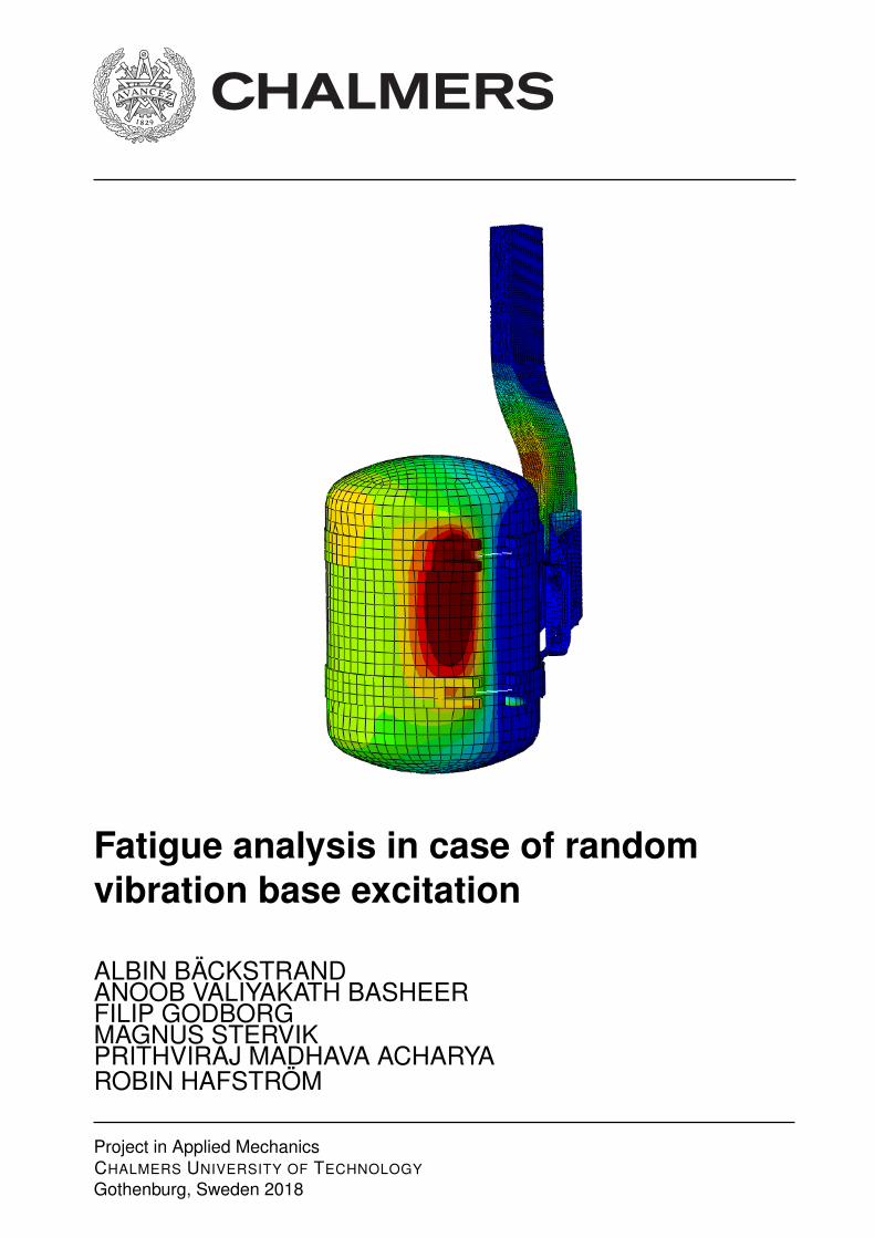
The figure on the front page shows a FE-model of an air tank, found underneath atypical Volvo truck chassis.

iv

1Introduction

1.1 BackgroundComponents mounted on truck chassis are subjected to random vibrations due tomovement of the base structure, which in long term causes material fatigue. Thecomponents have requirement specifications, which calls for fatigue analyses in orderto ensure sufficient operational lives. One way of doing this is by physical tests usingelectrodynamic shakers on hardware components. Since these tend to be both timeand cost consuming, it would be beneficial to do numerical fatigue analyses beforephysical tests. Doing this in time domain is often computationally heavy consider-ing high cycle fatigue. Hence, it would be more efficient to carry out the numericalanalysis in the frequency domain, which does not require time history inputs.

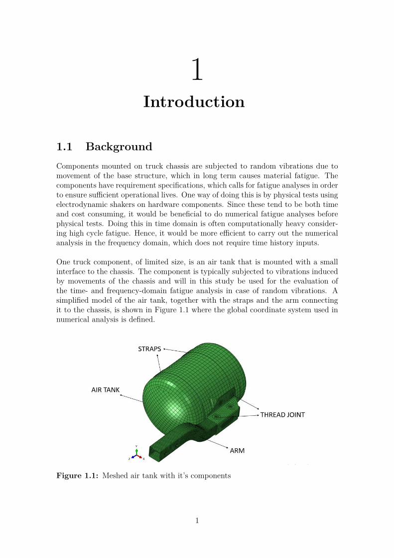
One truck component, of limited size, is an air tank that is mounted with a smallinterface to the chassis. The component is typically subjected to vibrations inducedby movements of the chassis and will in this study be used for the evaluation ofthe time- and frequency-domain fatigue analysis in case of random vibrations. Asimplified model of the air tank, together with the straps and the arm connectingit to the chassis, is shown in Figure 1.1 where the global coordinate system used innumerical analysis is defined.

Figure 1.1: Meshed air tank with it’s components

1

1. Introduction

1.2 PurposeThe purpose of this study is to understand and implement low-effort frequencydomain fatigue analyses instead of classical time domain fatigue analysis in case ofrandom vibration loads.

1.3 AimThe aim is to, under 8 study weeks, develop numerical tools for fatigue analysis inthe frequency domain and compare results with those obtained by well establishedtime-domain analyses. The accuracy of the two methods will be compared usingfatigue damage.

1.4 LimitationsAll analyses will be carried out for model (including geometry and mesh) providedby Volvo Trucks. The number of FE-nodes for the current mesh are limited to21309. Other mesh configurations will not be considered. Surface roughness, whichcan have an effect on the fatigue evaluation, will not be taken into account. Thematerial is assumed to be elastic so that no plastic deformation will be considered.Hence, non-linear effects due to deformation will be omitted. The amplitude of thevibration input load is assumed to have a Gaussian distribution with zero mean.

2

2Theory

This chapter presents the theoretical background for the studies.

2.1 Fatigue AnalysisIn order to estimate the fatigue life, S-N analysis in the form of Wöhler curve isused. Wöhler curve is a log-log diagram with the amplitude stresses, σa, plottedagainst the number of stress cycles to failure, Nf . [1]

In order to find the total damage of a component, the number of stress cycles,Ni = N(Si) for a given stress amplitude, Si, are evaluated against the number ofcycles to failure, Nf = Nf(Si), for that particular stress amplitude found from theWöhler curve. From the Palmgren−Miner rule, the total accumulated damage, Dtot,is expressed as the sum over the ratio between the number of stress cycles to thenumber of cycles to failure as

Dtot =∑

i

Ni

Nf=∑

i

N(Si)Nf(Si)

(2.1)

Since the accumulated damage is proportional to the damage required to failure, thefatigue life Tlife can be obtained as the ratio between the length of the time historyT and the accumulated damage presuming steady state process [2].

Tlife = T

Dtot(2.2)

2.1.1 Fatigue analysis in time domainRainflow counting is used to evaluate the stress cycles in the stress time historyin cases of varying amplitude. Fatigue damage corresponding to stress cycles areadded using the Palmgren−Miner rule (2.1) to calculate the accumulated damagein a material point. Fatigue failure is presumed when Dtot = 1.

2.1.2 Fatigue analysis in frequency domainIn frequency domain fatigue analysis, the information available is the input for thestress Power Spectral Density (PSD) matrix. Therefore the PSD has to be con-verted into an approximation of the number of stress cycles with respective stressamplitudes. See section 2.2 for more information on PSD.

3

2. Theory

One way to do this is by using Dirlik’s formula [2]:

N(S) = E[P ] · T · p(S) (2.3)

where N(S) is the density function between the number of cycles and stress range,S. E[P ] is the expected number of peaks per unit time and p(S) is a density functionof S. The initial step is to calculate the first, second, third and fourth moments ofarea of the PSD function. The nth moment of area is obtained by:

mn =∫ ∞

0fn ·G(f)df (2.4)

where G(f) is the value of the PSD at frequency f . From here, the expected numberof peaks per unit time, E[P ], is obtained by [2]

E[P ] =√m4

m2(2.5)

and

p(S) =D1Qe−Z/Q + D2Z

R2 e−Z2/2R2 +D3Ze

−Z2/2

2 · √m0(2.6)

With the mean frequency xm and the normalized amplitude Z defined as

xm = m1

m0

√m2

m4(2.7)

Z = S

2 · √m0(2.8)

The coefficients used in Equation (2.6) are defined in [2] as:

γ = m2√m0m4

(2.9)

D1 = 2 (xm − γ2)1 + γ2 (2.10)

D2 = 1− γ −D1 +D21

1−R (2.11)

D3 = 1−D1 −D2 (2.12)

Q = 1.25(γ −D3 −D2R)D1

(2.13)

R = γ − xm −D21

1− γ −D1 −D21

(2.14)

2.1.3 Multiaxial fatigue in frequency domainIn order to estimate fatigue damage for a multiaxial state of stress in frequencydomain, it is convenient to reduce the problem into a simple equivalent uniaxialstress state. The intention is to convert a general multiaxial stress problem with 6

4

2. Theory

stress components, σij, into an equivalent stress scalar σeq before applying Dirlik’sformula. In this project the von Mises stress was used, defined as

σ2eq = 1

2(σ11 − σ22)2 + 12(σ22 − σ33)2 + 1

2(σ11 − σ33)2 + 3(σ212 + σ2

13 + σ223)

= sT ·Q · s = trace{Q · ssT}(2.15)

where

s =[σ11 σ12 σ13 σ22 σ23 σ33

]T,

Q =

1 0 0 0 0 00 3 0 0 0 00 0 3 0 0 0−1 0 0 1 0 00 0 0 0 3 0−1 0 0 −1 0 1

(2.16)

By assuming that the mean value of the stress components are zero and by usingthe fact that the trace operator is linear, it can be shown from Equation (2.15) thatthe PSD of the equivalent von Mises stress Geq(f) is given as

Geq(f) = trace{Q ·Gss(f)} (2.17)

where Gss(f) is the PSD of the matrix ssT [3].

2.2 Power spectral densityIn order to transform from the time domain to the frequency domain, a PSD is used.Halfpenny shows in [4] that a PSD is a statistical way of representing the amplitudecontent of a signal. The first step is to do a fast Fourier transform of the time signal.This is done by using Equation 2.18

y(fn) = 2TN

∑k

y(tk)e−i 2πnN

k (2.18)

where T is the period time, tk is the discrete time, y(tk) is the time history input,N is the number of data points in the history signal and fn = n

Trepresents the

discrete frequency [4]. y(fn) is now the signal in the frequency domain and the PSDis defined as

G(f) = 12T y(f) · y∗(f) = 1

2T |y(f)|2 (2.19)

The area under the PSD curve represents the mean square amplitude of the signal.

2.3 Transfer functionFor a linear system in the frequency domain, one can estimate the relation betweeninput load x(f) and output response y(f) by using a transfer function h(f) asfollows:

y(f) = h(f) · x(f) (2.20)

5

2. Theory

In this study, the estimation of the stress response, sij(f), is required for givenevaluation points on the model when applying an uniaxial acceleration load a(f).In general, there are 6 stress components, each one corresponding to a transferfunction. Hence, the relation between the stress vector s(f) and the accelerationload a(f) is given as

s(f) = h(f) · a(f) (2.21)

where h(f) is the transfer function vector. Furthermore, in order to obtain the PSDmatrix Gss(f) Equation (2.17), the definition of the PSD, according to Equation(2.19), can be expressed as follows:

Gss(f) = 12T s(f) · s∗T (f) = 1

2T (h(f) · a(f)) · (h∗T (f) · a∗(f))

= h(f) · h∗T (f)︸ ︷︷ ︸=H(f)

· 12T |a(f)|2︸ ︷︷ ︸

=Ga(f)

= H(f) ·Ga(f) (2.22)

where H(f) = h(f) ·h∗T (f) is the transfer function between the PSD of accelerationload Ga(f) and Gss(f).

It follows directly from the definition of H(f) that the diagonal components arealways real positive values while the off-diagonal components are in general com-plex valued. This can be verified by rewriting H(f) in index notation; Hij = hih

∗j ,

where i = j gives Hii = hih∗i = |hi|2. The complex off-diagonal components repre-

sent a phase difference between the stress components caused by propagation delaysin the material.

6

3Method

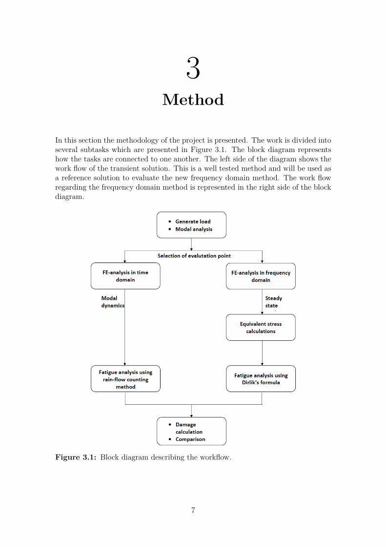
In this section the methodology of the project is presented. The work is divided intoseveral subtasks which are presented in Figure 3.1. The block diagram representshow the tasks are connected to one another. The left side of the diagram shows thework flow of the transient solution. This is a well tested method and will be used asa reference solution to evaluate the new frequency domain method. The work flowregarding the frequency domain method is represented in the right side of the blockdiagram.

Figure 3.1: Block diagram describing the workflow.

7

3. Method

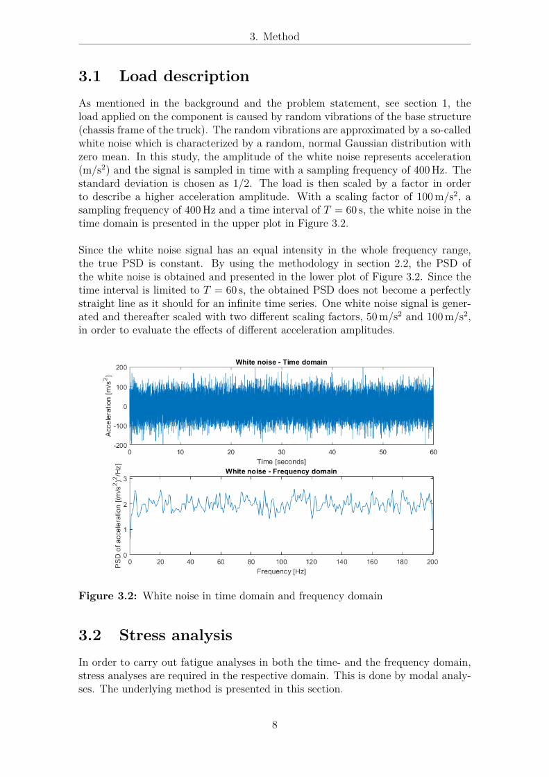
3.1 Load descriptionAs mentioned in the background and the problem statement, see section 1, theload applied on the component is caused by random vibrations of the base structure(chassis frame of the truck). The random vibrations are approximated by a so-calledwhite noise which is characterized by a random, normal Gaussian distribution withzero mean. In this study, the amplitude of the white noise represents acceleration(m/s2) and the signal is sampled in time with a sampling frequency of 400Hz. Thestandard deviation is chosen as 1/2. The load is then scaled by a factor in orderto describe a higher acceleration amplitude. With a scaling factor of 100 m/s2, asampling frequency of 400 Hz and a time interval of T = 60 s, the white noise in thetime domain is presented in the upper plot in Figure 3.2.

Since the white noise signal has an equal intensity in the whole frequency range,the true PSD is constant. By using the methodology in section 2.2, the PSD ofthe white noise is obtained and presented in the lower plot of Figure 3.2. Since thetime interval is limited to T = 60 s, the obtained PSD does not become a perfectlystraight line as it should for an infinite time series. One white noise signal is gener-ated and thereafter scaled with two different scaling factors, 50 m/s2 and 100 m/s2,in order to evaluate the effects of different acceleration amplitudes.

Figure 3.2: White noise in time domain and frequency domain

3.2 Stress analysisIn order to carry out fatigue analyses in both the time- and the frequency domain,stress analyses are required in the respective domain. This is done by modal analy-ses. The underlying method is presented in this section.

8

3. Method

3.2.1 Numerical model & constraintsThe geometry of the component, shown in Figure 1.1 in section 1.1, is provided byVolvo Trucks, and is described by shell elements. The finite elements used are ofshell type. Details about the FE-mesh from the commercial software ABAQUS [5]are presented in Table 3.1.

Table 3.1: Mesh details

Number of nodes 21 309Number of elements 21 302

B31 (2-node linear beam)Element types [5] S4 (4-node shell element)

S3R (3-node shell element with reduced integration)

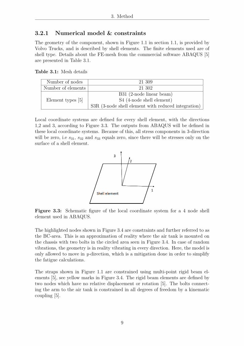
Local coordinate systems are defined for every shell element, with the directions1,2 and 3, according to Figure 3.3. The outputs from ABAQUS will be defined inthese local coordinate systems. Because of this, all stress components in 3-directionwill be zero, i.e s31, s32 and s33 equals zero, since there will be stresses only on thesurface of a shell element.

Figure 3.3: Schematic figure of the local coordinate system for a 4 node shellelement used in ABAQUS.

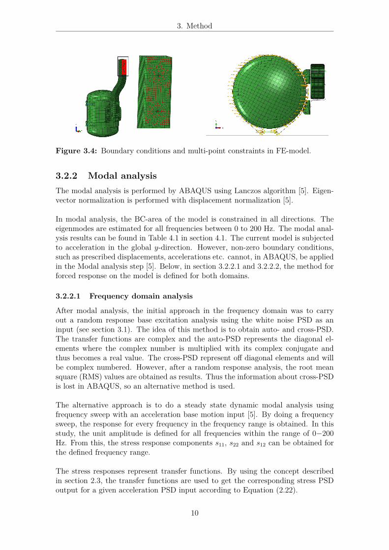
The highlighted nodes shown in Figure 3.4 are constraints and further referred to asthe BC-area. This is an approximation of reality where the air tank is mounted onthe chassis with two bolts in the circled area seen in Figure 3.4. In case of randomvibrations, the geometry is in reality vibrating in every direction. Here, the model isonly allowed to move in y-direction, which is a mitigation done in order to simplifythe fatigue calculations.

The straps shown in Figure 1.1 are constrained using multi-point rigid beam el-ements [5], see yellow marks in Figure 3.4. The rigid beam elements are defined bytwo nodes which have no relative displacement or rotation [5]. The bolts connect-ing the arm to the air tank is constrained in all degrees of freedom by a kinematiccoupling [5].

9

3. Method

Figure 3.4: Boundary conditions and multi-point constraints in FE-model.

3.2.2 Modal analysisThe modal analysis is performed by ABAQUS using Lanczos algorithm [5]. Eigen-vector normalization is performed with displacement normalization [5].

In modal analysis, the BC-area of the model is constrained in all directions. Theeigenmodes are estimated for all frequencies between 0 to 200 Hz. The modal anal-ysis results can be found in Table 4.1 in section 4.1. The current model is subjectedto acceleration in the global y-direction. However, non-zero boundary conditions,such as prescribed displacements, accelerations etc. cannot, in ABAQUS, be appliedin the Modal analysis step [5]. Below, in section 3.2.2.1 and 3.2.2.2, the method forforced response on the model is defined for both domains.

3.2.2.1 Frequency domain analysis

After modal analysis, the initial approach in the frequency domain was to carryout a random response base excitation analysis using the white noise PSD as aninput (see section 3.1). The idea of this method is to obtain auto- and cross-PSD.The transfer functions are complex and the auto-PSD represents the diagonal el-ements where the complex number is multiplied with its complex conjugate andthus becomes a real value. The cross-PSD represent off diagonal elements and willbe complex numbered. However, after a random response analysis, the root meansquare (RMS) values are obtained as results. Thus the information about cross-PSDis lost in ABAQUS, so an alternative method is used.

The alternative approach is to do a steady state dynamic modal analysis usingfrequency sweep with an acceleration base motion input [5]. By doing a frequencysweep, the response for every frequency in the frequency range is obtained. In thisstudy, the unit amplitude is defined for all frequencies within the range of 0−200Hz. From this, the stress response components s11, s22 and s12 can be obtained forthe defined frequency range.

The stress responses represent transfer functions. By using the concept describedin section 2.3, the transfer functions are used to get the corresponding stress PSDoutput for a given acceleration PSD input according to Equation (2.22).

10

3. Method

3.2.2.2 Time domain analysis

For the time domain analysis, there are two different approaches for obtaining thestress response, of which one includes to first carry out a dynamic explicit analysisusing acceleration time series applied as an input load [5]. This method requireslarge computational time. The second method, used in this study, is to carry outa modal dynamic analysis after the modal analysis step explained above [5]. Theacceleration in y-direction is defined as a base acceleration in the modal dynamicanalysis step [5]. The resulting stresses obtained are used to estimate the fatiguelife of the component as explained in section 2.1.1.

3.2.3 Selection of evaluation pointsFrom the stress analyses, four different elements are selected for further evaluation.An element is evaluated rather than a node, since this gives continuous stresses forall frequencies and time steps. The resulting stresses are determined as an averageof the four stresses in Gaussian integration points in the shell element. One of theselected element experience multiaxial state of stress which means that none of theprincipal stresses are dominating. The other three points are in a state of uniaxialstress, which means that one principal stress is dominating the other. When choos-ing elements, singularity points, for example constrained points, are avoided sincethe results here can be unrealistic.

Each element has three local stress components s11, s12 and s22. The principalstresses are then obtain as

s1,2 = s11 + s22

2 ±√(

s11 − s22

2

)2+ s2

12 (3.1)

Only one non-zero principal stress exist for uniaxial stress state. It can be shownfrom (3.1) that this occur when

− s11 is dominant: s22 = s12 = 0,− s22 is dominant: s11 = s12 = 0,− normal stresses are in phase and equal in size: s11 = s22, s12 = 0

3.3 Fatigue analysis

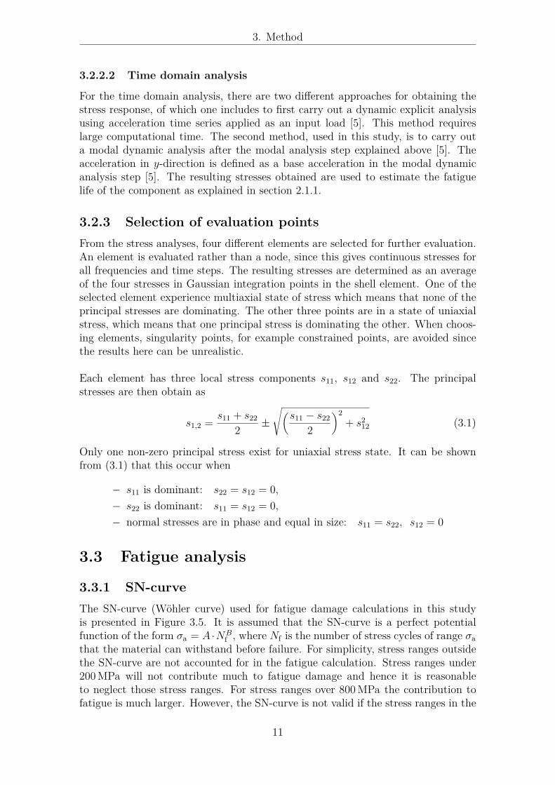
3.3.1 SN-curveThe SN-curve (Wöhler curve) used for fatigue damage calculations in this studyis presented in Figure 3.5. It is assumed that the SN-curve is a perfect potentialfunction of the form σa = A ·NB

f , where Nf is the number of stress cycles of range σathat the material can withstand before failure. For simplicity, stress ranges outsidethe SN-curve are not accounted for in the fatigue calculation. Stress ranges under200 MPa will not contribute much to fatigue damage and hence it is reasonableto neglect those stress ranges. For stress ranges over 800 MPa the contribution tofatigue is much larger. However, the SN-curve is not valid if the stress ranges in the

11

3. Method

given evaluation points exceeds 800 MPa. One reason is that plastic deformationswill occur and the presumptions for the SN-curve will no longer be valid.

Figure 3.5: Logarithmic plot of the SN-curve employed in the analysis.

3.3.2 Fatigue analysis in the time domainThe fatigue analyses in the time domain are performed based on a time historystress. The built-in MATLAB function rainflow is then used to calculate the num-ber of cycles for different stress ranges. Then to calculate fatigue damage and fatiguelife Equations (2.1) and (2.2) are used, respectively.

The rainflow-count is preformed on the largest (most dominant) stress component,not on the equivalent von Mises stress as in Dirlik’s formula. This because it’sdifficult to apply the rainflow-count algorithm on multiaxial state stresses.

3.3.3 Fatigue analysis in the frequency domainAs mentioned in section 3.2.2.1, the stress responses that represent the transfer func-tions are obtained from ABAQUS through steady state dynamic modal analysis inthe frequency domain. The stress PSD can then be obtained through Equations(2.21) and (2.22). The fatigue analysis in the frequency domain is done using thismethod to obtain the stress PSD. The stress PSD is applied in Dirlik’s method inorder to calculate the number of cycles for a given stress interval, see Equation (2.3).For the estimated number of cycles per given stress interval the damage and fatiguelife are obtained by Equation 2.1 and 2.2 respectively.

If the stress state is multiaxial, a PSD for the equivalent von Mises stress, as definedin Equation (2.17), has to be calculated in order to use it in Dirlik’s method.

12

4Results and discussion

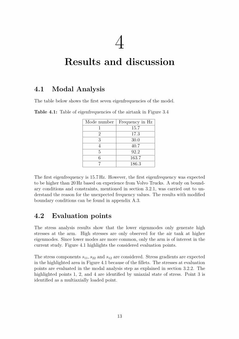
4.1 Modal AnalysisThe table below shows the first seven eigenfrequencies of the model.

Table 4.1: Table of eigenfrequencies of the airtank in Figure 3.4

Mode number Frequency in Hz1 15.72 17.33 30.04 40.75 92.26 163.77 186.3

The first eigenfrequency is 15.7Hz. However, the first eigenfrequency was expectedto be higher than 20Hz based on experience from Volvo Trucks. A study on bound-ary conditions and constraints, mentioned in section 3.2.1, was carried out to un-derstand the reason for the unexpected frequency values. The results with modifiedboundary conditions can be found in appendix A.3.

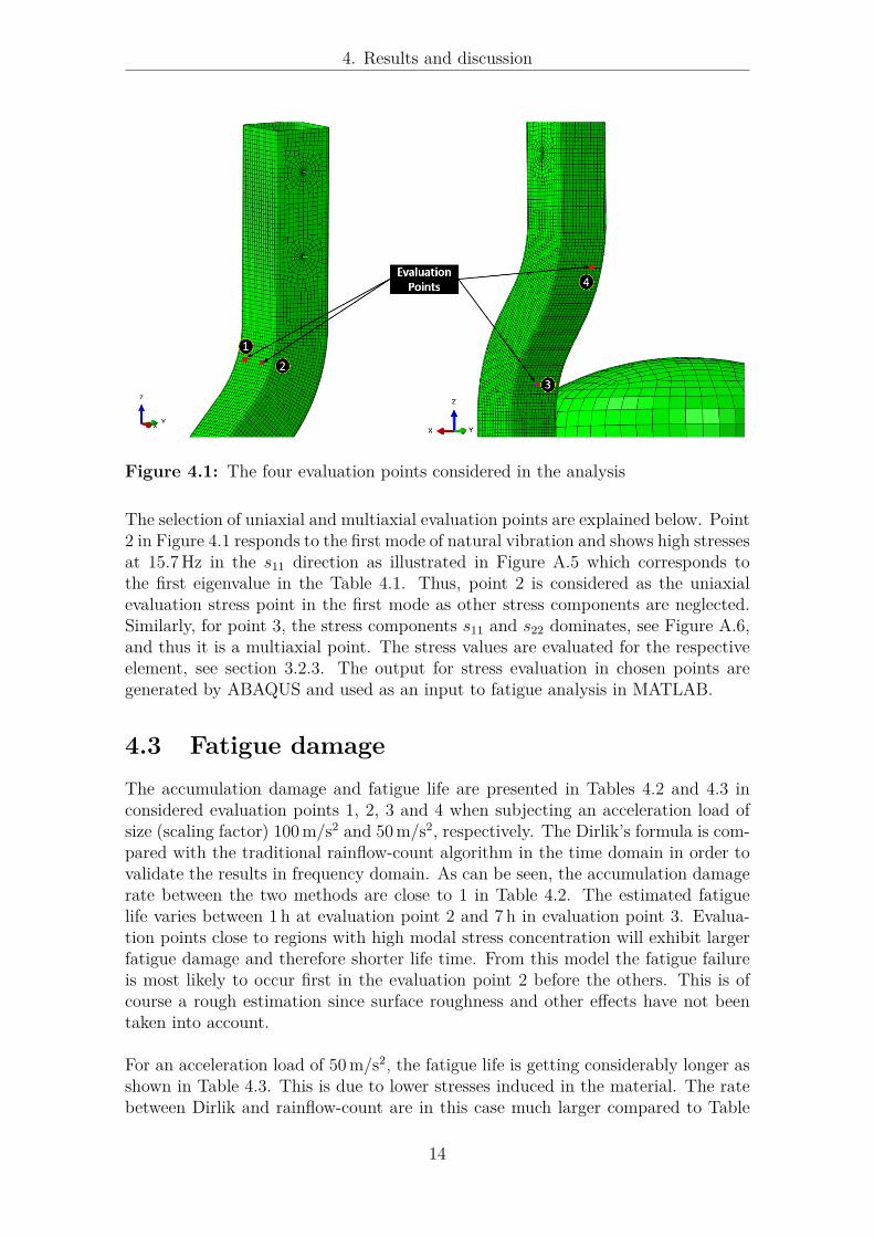
4.2 Evaluation pointsThe stress analysis results show that the lower eigenmodes only generate highstresses at the arm. High stresses are only observed for the air tank at highereigenmodes. Since lower modes are more common, only the arm is of interest in thecurrent study. Figure 4.1 highlights the considered evaluation points.

The stress components s11, s22 and s12 are considered. Stress gradients are expectedin the highlighted area in Figure 4.1 because of the fillets. The stresses at evaluationpoints are evaluated in the modal analysis step as explained in section 3.2.2. Thehighlighted points 1, 2, and 4 are identified by uniaxial state of stress. Point 3 isidentified as a multiaxially loaded point.

13

4. Results and discussion

Figure 4.1: The four evaluation points considered in the analysis

The selection of uniaxial and multiaxial evaluation points are explained below. Point2 in Figure 4.1 responds to the first mode of natural vibration and shows high stressesat 15.7Hz in the s11 direction as illustrated in Figure A.5 which corresponds tothe first eigenvalue in the Table 4.1. Thus, point 2 is considered as the uniaxialevaluation stress point in the first mode as other stress components are neglected.Similarly, for point 3, the stress components s11 and s22 dominates, see Figure A.6,and thus it is a multiaxial point. The stress values are evaluated for the respectiveelement, see section 3.2.3. The output for stress evaluation in chosen points aregenerated by ABAQUS and used as an input to fatigue analysis in MATLAB.

4.3 Fatigue damageThe accumulation damage and fatigue life are presented in Tables 4.2 and 4.3 inconsidered evaluation points 1, 2, 3 and 4 when subjecting an acceleration load ofsize (scaling factor) 100 m/s2 and 50 m/s2, respectively. The Dirlik’s formula is com-pared with the traditional rainflow-count algorithm in the time domain in order tovalidate the results in frequency domain. As can be seen, the accumulation damagerate between the two methods are close to 1 in Table 4.2. The estimated fatiguelife varies between 1 h at evaluation point 2 and 7 h in evaluation point 3. Evalua-tion points close to regions with high modal stress concentration will exhibit largerfatigue damage and therefore shorter life time. From this model the fatigue failureis most likely to occur first in the evaluation point 2 before the others. This is ofcourse a rough estimation since surface roughness and other effects have not beentaken into account.

For an acceleration load of 50 m/s2, the fatigue life is getting considerably longer asshown in Table 4.3. This is due to lower stresses induced in the material. The ratebetween Dirlik and rainflow-count are in this case much larger compared to Table

14

4. Results and discussion

4.2. The reason for this is probably the short length of the time history (T = 60 s)which will give a significant instability in the results. Further, the number of cyclecounts inside the SN-curve range are reduced which will contribute to even moreinstability (the SN-curve is a potential function and small stress range errors caneasily result in even larger damage errors).

The length of the time history is also a problem in frequency domain since thePSD, which in theory should be constant for white noise, is not really a straight line(see Figure 3.2). This gives an instability since the PSD of the white noise will lookslightly different when the noise is generated. The best would be to have a muchlonger sampling history (infinitely long in theory), but the problem occurs whenrunning the transient analysis in ABAQUS, since it would require much heaviercomputer simulations.

The acceleration load of scaling factor 100 m/s2 turned out to be an unrealisticload since the estimated fatigue life is only a couple of hours. By reducing the loadsize one can approach a much more realistic vibration load of the chassis frame.Other scaling factors were not considered, since the aim of the particular projectwas to validate fatigue damage in frequency domain using Dirlik’s method.

The multiaxial stress state in evaluation points 3 are dominated by the local stresscomponents s11 and s22 (see Appendix A.2). The stresses are in phase with zeromean which makes it possible to apply von Mises equivalent stress since the peaksof the equivalent stress occur at the same intervals of time as for s11 and s22, butwith increased amplitude. However, the rainflow-count algorithm is hard to imple-ment for multiaxial stress state and hence it was only used for the largest stresscomponent, which of course effects the results in the time domain.

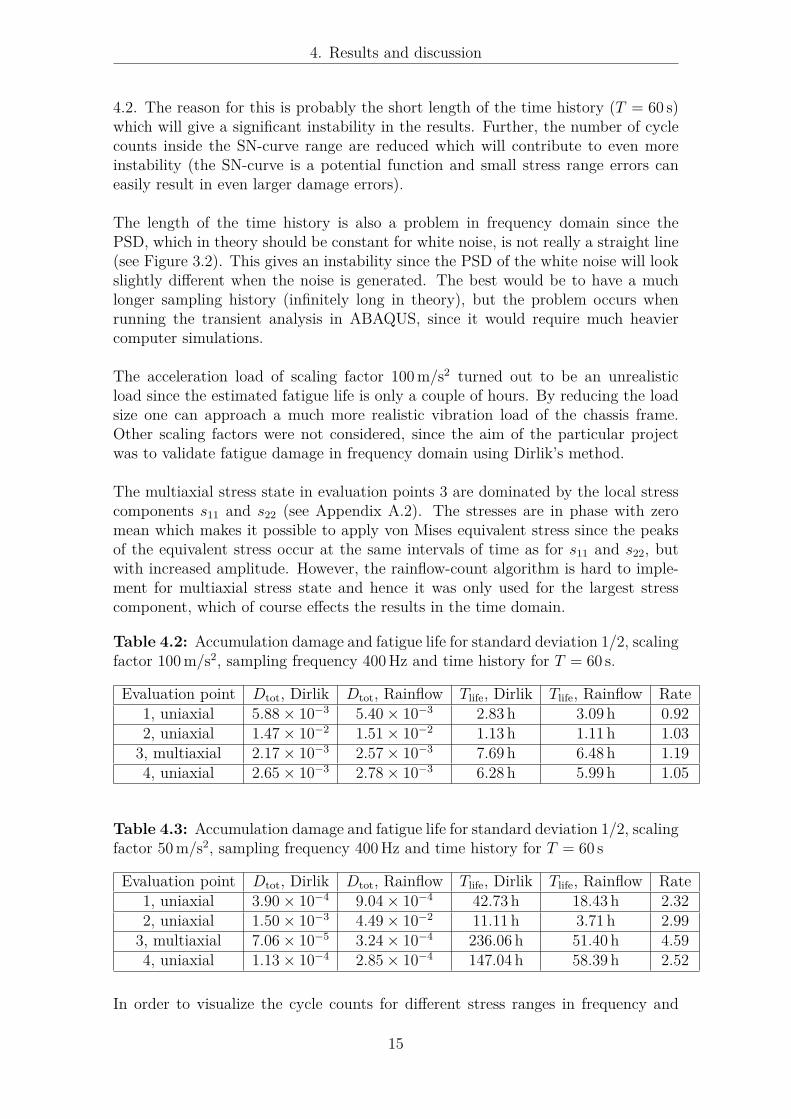
Table 4.2: Accumulation damage and fatigue life for standard deviation 1/2, scalingfactor 100 m/s2, sampling frequency 400 Hz and time history for T = 60 s.

Evaluation point Dtot, Dirlik Dtot, Rainflow Tlife, Dirlik Tlife, Rainflow Rate1, uniaxial 5.88× 10−3 5.40× 10−3 2.83 h 3.09 h 0.922, uniaxial 1.47× 10−2 1.51× 10−2 1.13 h 1.11 h 1.033, multiaxial 2.17× 10−3 2.57× 10−3 7.69 h 6.48 h 1.194, uniaxial 2.65× 10−3 2.78× 10−3 6.28 h 5.99 h 1.05

Table 4.3: Accumulation damage and fatigue life for standard deviation 1/2, scalingfactor 50 m/s2, sampling frequency 400 Hz and time history for T = 60 s

Evaluation point Dtot, Dirlik Dtot, Rainflow Tlife, Dirlik Tlife, Rainflow Rate1, uniaxial 3.90× 10−4 9.04× 10−4 42.73 h 18.43 h 2.322, uniaxial 1.50× 10−3 4.49× 10−2 11.11 h 3.71 h 2.993, multiaxial 7.06× 10−5 3.24× 10−4 236.06 h 51.40 h 4.594, uniaxial 1.13× 10−4 2.85× 10−4 147.04 h 58.39 h 2.52

In order to visualize the cycle counts for different stress ranges in frequency and

15

4. Results and discussion

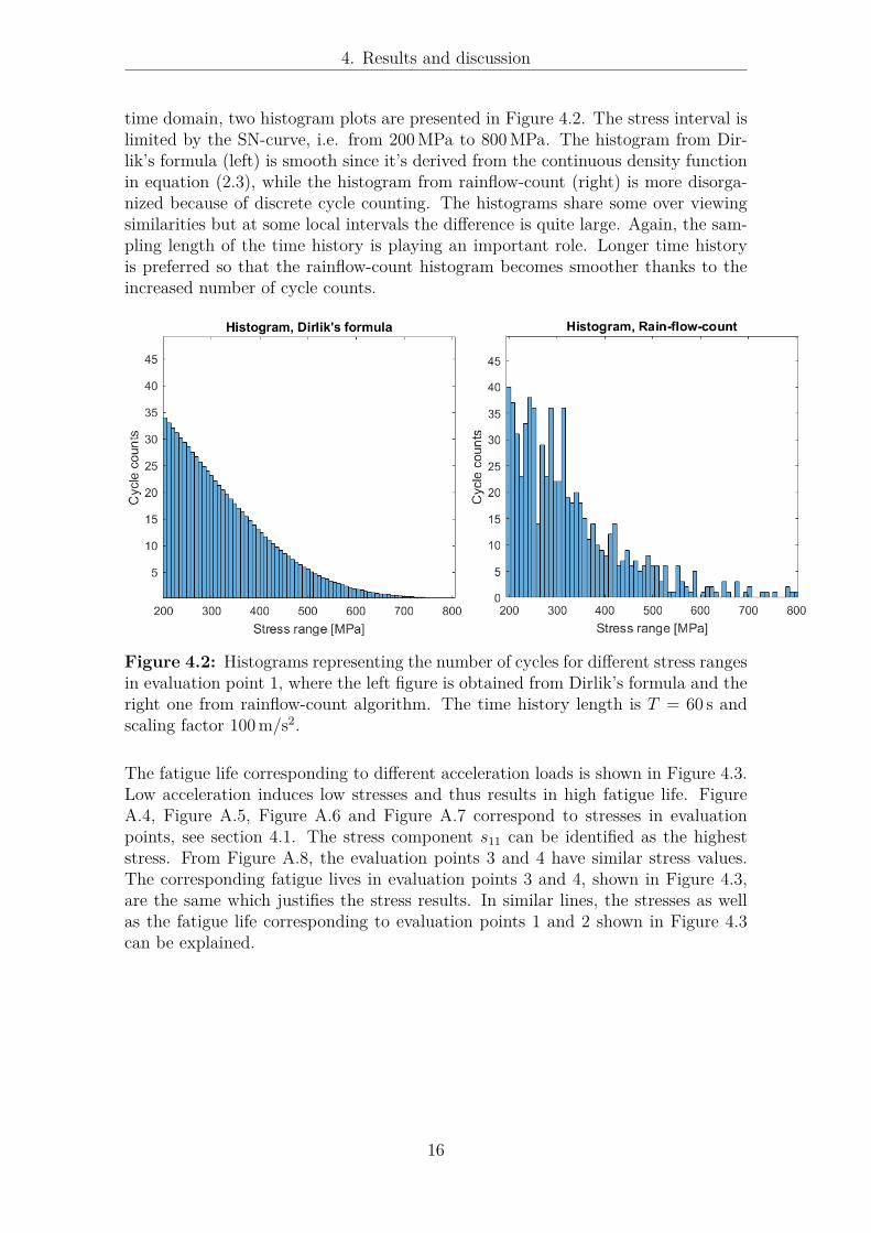
time domain, two histogram plots are presented in Figure 4.2. The stress interval islimited by the SN-curve, i.e. from 200 MPa to 800 MPa. The histogram from Dir-lik’s formula (left) is smooth since it’s derived from the continuous density functionin equation (2.3), while the histogram from rainflow-count (right) is more disorga-nized because of discrete cycle counting. The histograms share some over viewingsimilarities but at some local intervals the difference is quite large. Again, the sam-pling length of the time history is playing an important role. Longer time historyis preferred so that the rainflow-count histogram becomes smoother thanks to theincreased number of cycle counts.

Figure 4.2: Histograms representing the number of cycles for different stress rangesin evaluation point 1, where the left figure is obtained from Dirlik’s formula and theright one from rainflow-count algorithm. The time history length is T = 60 s andscaling factor 100 m/s2.

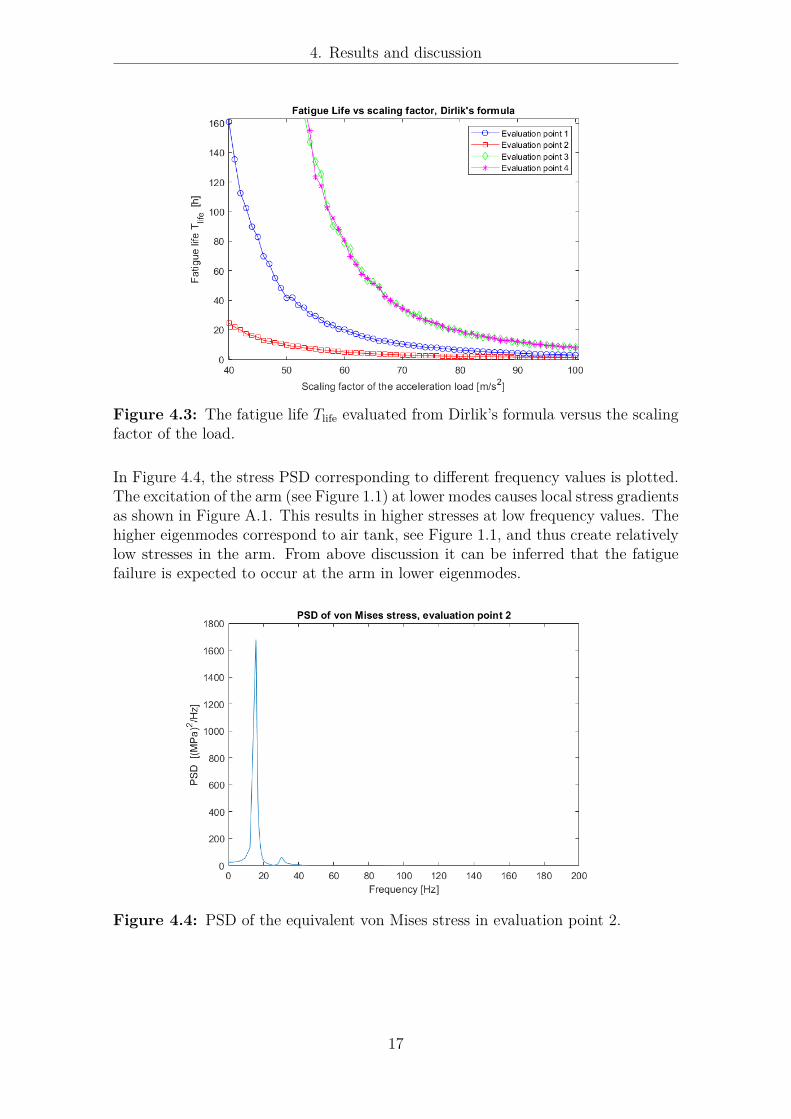
The fatigue life corresponding to different acceleration loads is shown in Figure 4.3.Low acceleration induces low stresses and thus results in high fatigue life. FigureA.4, Figure A.5, Figure A.6 and Figure A.7 correspond to stresses in evaluationpoints, see section 4.1. The stress component s11 can be identified as the higheststress. From Figure A.8, the evaluation points 3 and 4 have similar stress values.The corresponding fatigue lives in evaluation points 3 and 4, shown in Figure 4.3,are the same which justifies the stress results. In similar lines, the stresses as wellas the fatigue life corresponding to evaluation points 1 and 2 shown in Figure 4.3can be explained.

16

4. Results and discussion

Figure 4.3: The fatigue life Tlife evaluated from Dirlik’s formula versus the scalingfactor of the load.

In Figure 4.4, the stress PSD corresponding to different frequency values is plotted.The excitation of the arm (see Figure 1.1) at lower modes causes local stress gradientsas shown in Figure A.1. This results in higher stresses at low frequency values. Thehigher eigenmodes correspond to air tank, see Figure 1.1, and thus create relativelylow stresses in the arm. From above discussion it can be inferred that the fatiguefailure is expected to occur at the arm in lower eigenmodes.

Figure 4.4: PSD of the equivalent von Mises stress in evaluation point 2.

17

5Conclusions and future work

As expected, the frequency domain analyses are more efficient in the sense that theydo not require large computational data in form of time history inputs and outputsas the time domain analyses do. Also, in order to carry out a time-domain analysis,new FE-analyses are required for every new input signal. By carrying out the anal-yses in the frequency domain, transfer functions are obtained for all frequencies. Byusing the transfer functions, for example in MATLAB, stresses can be obtained bymultiplying them with the input PSD signal. This means that only one FE-analysisis required.

The results show that the frequency domain fatigue analysis is useful in early phasedevelopment, because of it’s effectiveness. Although, it might not be considered agood idea to use it in final evaluations, since it’s not as accurate as the time domainanalysis. One should remember that the results in this study are based on onlyone component geometry, a very high acceleration amplitude and only four differentevaluation points. Therefore, other configuration should be tested in order to vali-date the results.

The time history used in this project was shortened to only 60 seconds in order tosave time and computer power when running the FE-simulations in time domain.Short time history results in a less accurate fatigue life. Hence it’s preferable to usemuch longer time history even though it would require more computer power.

18

Bibliography

[1] A. Ekberg, “Materialutmattning,” 2017.[2] A. Halfpenny, “A frequency domain approach for fatigue life estimation from

Finite Element Analysis,” 1999.[3] A. P. X. Pitoiset, “Spectral methods for multiaxial random fatigue analysis of

metallic structures,” 2000.[4] D. A. Halfpenny, “What is the ’Frequency Domain’ and how do we use a PSD?”

1999.[5] Abaqus documentation. SIMULIA. [Online]. Tillgänglig: file:///C:

/Program%20Files/Dassault%20Systemes/SIMULIA2017doc/English/DSSIMULIA_Established.htm

[6] Matlab documentation. Mathworks. [Online]. Tillgänglig: https://www.mathworks.com/help/matlab/ref/fft.html

19

AAppendix

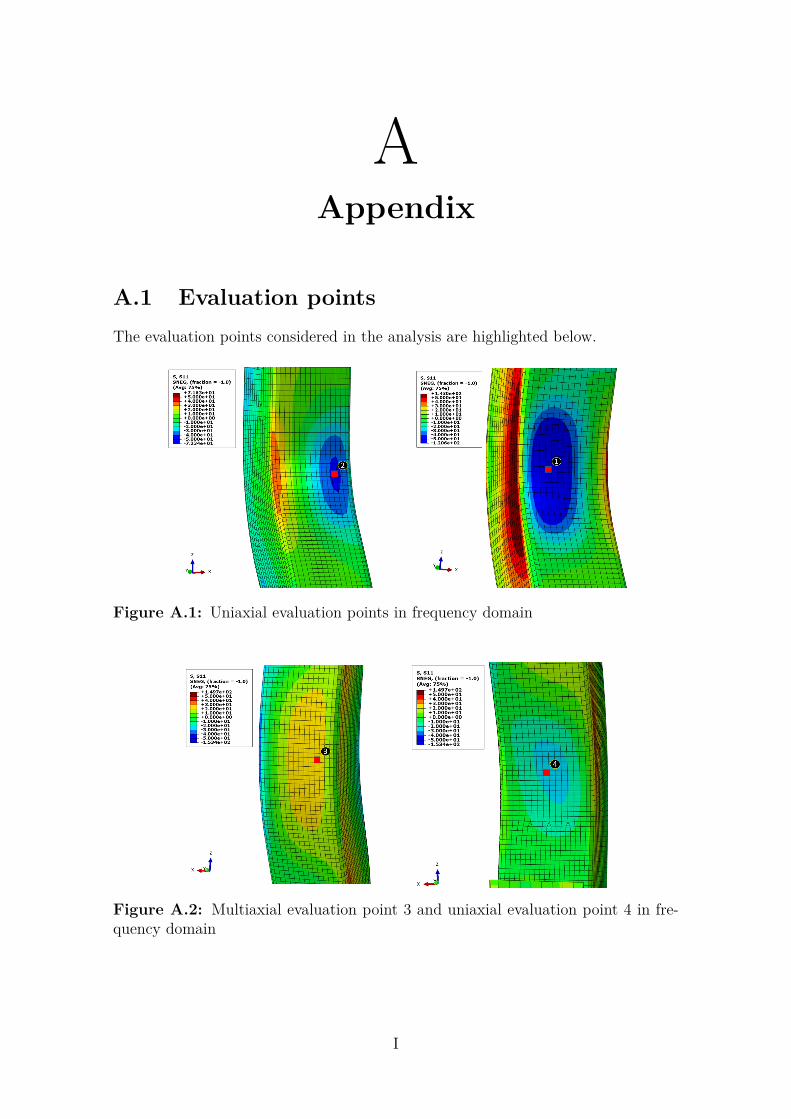
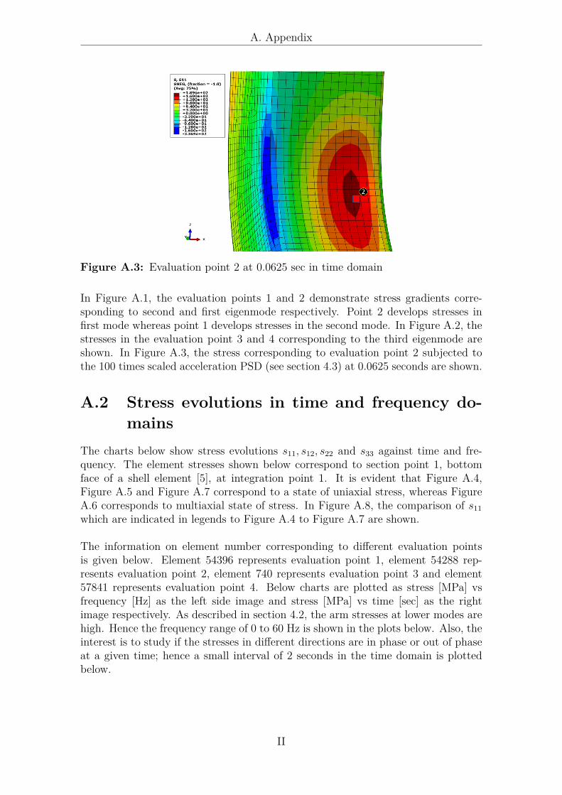
A.1 Evaluation pointsThe evaluation points considered in the analysis are highlighted below.

Figure A.1: Uniaxial evaluation points in frequency domain

Figure A.2: Multiaxial evaluation point 3 and uniaxial evaluation point 4 in fre-quency domain

I

A. Appendix

Figure A.3: Evaluation point 2 at 0.0625 sec in time domain

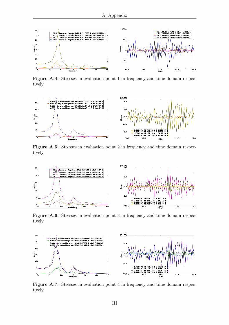
In Figure A.1, the evaluation points 1 and 2 demonstrate stress gradients corre-sponding to second and first eigenmode respectively. Point 2 develops stresses infirst mode whereas point 1 develops stresses in the second mode. In Figure A.2, thestresses in the evaluation point 3 and 4 corresponding to the third eigenmode areshown. In Figure A.3, the stress corresponding to evaluation point 2 subjected tothe 100 times scaled acceleration PSD (see section 4.3) at 0.0625 seconds are shown.

A.2 Stress evolutions in time and frequency do-mains

The charts below show stress evolutions s11, s12, s22 and s33 against time and fre-quency. The element stresses shown below correspond to section point 1, bottomface of a shell element [5], at integration point 1. It is evident that Figure A.4,Figure A.5 and Figure A.7 correspond to a state of uniaxial stress, whereas FigureA.6 corresponds to multiaxial state of stress. In Figure A.8, the comparison of s11which are indicated in legends to Figure A.4 to Figure A.7 are shown.

The information on element number corresponding to different evaluation pointsis given below. Element 54396 represents evaluation point 1, element 54288 rep-resents evaluation point 2, element 740 represents evaluation point 3 and element57841 represents evaluation point 4. Below charts are plotted as stress [MPa] vsfrequency [Hz] as the left side image and stress [MPa] vs time [sec] as the rightimage respectively. As described in section 4.2, the arm stresses at lower modes arehigh. Hence the frequency range of 0 to 60 Hz is shown in the plots below. Also, theinterest is to study if the stresses in different directions are in phase or out of phaseat a given time; hence a small interval of 2 seconds in the time domain is plottedbelow.

II

A. Appendix

Figure A.4: Stresses in evaluation point 1 in frequency and time domain respec-tively

Figure A.5: Stresses in evaluation point 2 in frequency and time domain respec-tively

Figure A.6: Stresses in evaluation point 3 in frequency and time domain respec-tively

Figure A.7: Stresses in evaluation point 4 in frequency and time domain respec-tively

III

A. Appendix

Figure A.8: Stress s11 at evaluation points in frequency and time domain respec-tively

A.3 Effect of constraints on frequency

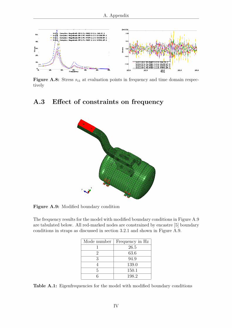
Figure A.9: Modified boundary condition

The frequency results for the model with modified boundary conditions in Figure A.9are tabulated below. All red-marked nodes are constrained by encastre [5] boundaryconditions in straps as discussed in section 3.2.1 and shown in Figure A.9.

Mode number Frequency in Hz1 26.52 63.63 94.94 139.05 150.16 198.2

Table A.1: Eigenfrequencies for the model with modified boundary conditions

IV