Fat Chance! Obesity and the Transition from …ftp.iza.org/dp5795.pdf · Fat Chance! Obesity and...
35
DISCUSSION PAPER SERIES Forschungsinstitut zur Zukunft der Arbeit Institute for the Study of Labor Fat Chance! Obesity and the Transition from Unemployment to Employment IZA DP No. 5795 June 2011 Marco Caliendo Wang-Sheng Lee
Transcript of Fat Chance! Obesity and the Transition from …ftp.iza.org/dp5795.pdf · Fat Chance! Obesity and...

DI
SC
US
SI
ON
P
AP
ER
S
ER
IE
S
Forschungsinstitut zur Zukunft der ArbeitInstitute for the Study of Labor
Fat Chance! Obesity and the Transition fromUnemployment to Employment
IZA DP No. 5795
June 2011
Marco CaliendoWang-Sheng Lee

Fat Chance!
Obesity and the Transition from Unemployment to Employment
Marco Caliendo IZA, IAB and DIW Berlin
Wang-Sheng Lee RMIT University and IZA
Discussion Paper No. 5795 June 2011
IZA
P.O. Box 7240 53072 Bonn
Germany
Phone: +49-228-3894-0 Fax: +49-228-3894-180
E-mail: [email protected]
Any opinions expressed here are those of the author(s) and not those of IZA. Research published in this series may include views on policy, but the institute itself takes no institutional policy positions. The Institute for the Study of Labor (IZA) in Bonn is a local and virtual international research center and a place of communication between science, politics and business. IZA is an independent nonprofit organization supported by Deutsche Post Foundation. The center is associated with the University of Bonn and offers a stimulating research environment through its international network, workshops and conferences, data service, project support, research visits and doctoral program. IZA engages in (i) original and internationally competitive research in all fields of labor economics, (ii) development of policy concepts, and (iii) dissemination of research results and concepts to the interested public. IZA Discussion Papers often represent preliminary work and are circulated to encourage discussion. Citation of such a paper should account for its provisional character. A revised version may be available directly from the author.

IZA Discussion Paper No. 5795 June 2011
ABSTRACT
Fat Chance! Obesity and the Transition from Unemployment to Employment*
This paper focuses on estimating the magnitude of any potential weight discrimination by examining whether obese job applicants in Germany get treated or behave differently from non-obese applicants. Based on two waves of rich survey data from the IZA Evaluation dataset, which includes measures that control for education, demographic characteristics, labor market history, psychological factors and health, we estimate differences in job search behavior and labor market outcomes between obese/overweight and healthy weight individuals. Unlike other observational studies which are generally based on obese and non-obese individuals who might already be at different points in the job ladder (e.g., household surveys), in our data, individuals are newly unemployed and all start from the same point. The only subgroup we find in our data experiencing any possible form of labor market discrimination is obese women. Despite making more job applications and engaging more in job training programs, we find some indications that they experienced worse (or at best similar) employment outcomes than healthy weight women. Obese women who found a job also had significantly lower wages than healthy weight women. JEL Classification: I10, I12, J23, J70 Keywords: obesity, discrimination, employment, labor demand Corresponding author: Wang-Sheng Lee School of Economics, Finance and Marketing RMIT University Level 12 239 Bourke Street Victoria 3000 Australia E-mail: [email protected]
* The authors would like to thank Dan Hamermesh, seminar participants at RMIT University and Queensland University of Technology, and conference participants at the 3rd IZA Annual Conference on the Economics of Risky Behaviors for helpful comments and suggestions. The IAB (Nuremberg) kindly gave us permission to use the administrative data.
1. Introduction
Obesity has recently emerged as a prevalent problem in many developed
countries. For example, between the periods 1976-1980 and 1999-2000, the
prevalence of overweight (BMI ≥ 25) persons in the US increased from 46% to 65%,
and the prevalence of obesity (BMI ≥ 30) increased from 15% to 31% (Flegal et al.,
2002).1 By 2007-2008, the prevalence of obesity had further increased to 32.2%
among adult men and 35.5% among adult women (Flegal et al., 2010). Similarly in
Europe, the prevalence of obesity in men ranged from 4.0% to 28.3% and in women
from 6.2% to 36.5% during the period 1980-2005. Eastern Europe and the
Mediterranean countries showed higher prevalences of obesity than countries in
Western and Northern Europe (Berghöfer et al., 2008). The alarming rise of obesity
over the years has led to the practice of a new form of discrimination that has received
relatively little attention in the economics literature – weight discrimination.
Researchers estimate that at present, weight discrimination is comparable to
rates of race and age discrimination, especially among women. In 1995-96, weight
discrimination was reported by 7% of US adults. In 2004-2006, that percentage rose
to 12% of adults (Andreyeva et al., 2008). Puhl and Brownell (2001) published the
first comprehensive review of several decades of research documenting bias and
stigma toward overweight and obese persons. Their review summarized weight
stigma in domains of employment, health care, and education, demonstrating the
vulnerability of obese persons to many forms of unfair treatment. It highlighted that
weight discrimination is rampant in the workplace, health care and education arenas.
Based on data from the National Survey of Midlife Development in the US, a
nationally representative sample of adults aged 25–74 years, Roehling et al. (2007)
found that overweight respondents were 12 times more likely, obese respondents were
37 times more likely, and severely obese respondents were 100 times more likely than
normal-weight respondents to report employment discrimination. In addition, women
were 16 times more likely to report weight-related employment discrimination than
men. A meta-analysis of 32 experimental studies which investigated weight
discrimination in employment settings was recently conducted by Roehling et al.
(2008). Typically, such experimental studies ask participants to evaluate a fictional
applicant’s qualifications for a job, where his or her weight has been manipulated 1 Body mass index (BMI) is the ratio of weight measured in kilograms, to squared height measured in meters.
1
(through written vignettes, videos, photographs or computer morphing). Outcome
variables examined in these studies included hiring recommendations,
qualification/suitability ratings, disciplinary decisions, salary assignments, placement
decisions, and co-worker ratings. Across studies, it was demonstrated that overweight
job applicants and employees were evaluated more negatively and had more negative
employment outcomes compared to non-overweight applicants and employees.
This paper focuses on examining whether newly unemployed and obese job
applicants in Germany get treated or behave differently from non-obese applicants.
Despite evidence that obese people experience discrimination, to date, with the
exception of the state of Michigan in the US, which enacted a law in 1977 prohibiting
discrimination against overweight people, there are no laws protecting overweight
people from discrimination in employment, education, and health care. In Germany,
the 2006 General Equal Treatment Act (Allgemeines Gleichbehandlungsgesetz) was
introduced only after a long and controversial legislative procedure. This was
intended to be a combination of four EU Equality Directives (2000/43, 2000/78,
2002/73 and 2004/113) and prohibits discrimination based on race or ethnical origin,
religion or belief, sex, disability, age or sexual orientation. This paper examines more
closely whether these new laws had any effects on the outcomes of obese unemployed
Germans in 2007-2008.2 In addition to observing the employment outcomes of job
applicants, a novel feature of our data set is that we also have information on the
search behavior of job applicants. We therefore will be given insights as to whether
any observed differences in labor market outcomes have arisen because one group
simply was less motivated or tried less hard to look for a job, or possibly because they
had different access to labor market training programs.
To preview our findings, we find that overweight men, obese men and
overweight women experience no discrimination in terms of access to programs that
are part of active labor market policies (ALMP) or in their employment and wage
outcomes. The only group we find in our data experiencing any possible form of labor
market discrimination is obese women. Despite making more job applications and
engaging more in job training programs, we find some indications that they
experienced worse (or at best similar) employment outcomes than healthy weight
2 Discrimination against the obese is not explicitly mentioned in the 2006 Act but the new anti-discrimination culture in Germany could plausibly have indirect effects on them.
2
women. Obese women who found a job also had significantly lower wages than
healthy weight women.
The rest of this paper is organized as follows. Section 2 describes the data in
more detail. Section 3 provides more background and discusses some theoretical
motivations, whereas Section 4 presents the methods used. The empirical results are
provided in Section 5. Finally, Section 6 concludes.
2. Data
The IZA-Evaluation Dataset is an ongoing data collection process which is
specifically designed to shed more light on the transition process from unemployment
to employment (see Caliendo et al., 2011, for details). It consists of two components,
an administrative part as well as an additional survey data set. The sampling is
restricted to individuals who are 16 to 54 years old, and who receive or are eligible to
receive unemployment benefits under the German Social Code III. The administrative
part covers a random inflow sample into unemployment for the years 2001-2008
containing over 920,000 individuals. Administrative records are based on the
‘Integrated Labour Market Biographies’ of the Institute for Employment Research
(IAB), containing relevant register data from four sources: employment history,
unemployment support recipience, participation in active labor market programs, and
job seeker history. For the complementary survey a random sample of individuals
who entered unemployment between June 2007 and May 2008 is chosen. From the
monthly unemployment inflows of approximately 206,000 individuals in the
administrative records, a 9% random sample is drawn which constitutes the gross
sample. Out of this gross sample each month representative samples of approximately
1,450 individuals are interviewed, so that after one year 12 monthly cohorts are
gathered. The key feature of the data set is that individuals are interviewed shortly
after they become unemployed and are asked a variety of non-standard questions. In
addition to measuring an extensive set of individual-level characteristics and labor
market outcomes, a particular strength of the survey dataset is that it contains many
non-standard, innovative questions including search behavior, social networks,
psychological factors, cognitive and non-cognitive skills, subjective assessments on
future outcomes, and attitudes. As will be discussed in a later section, such rich
micro-level data are important in helping us identify the effects of obesity on labor
market outcomes using decomposition and matching approaches.
3

For the purposes of this paper, we focus on three cohorts of the survey dataset
(June 2007, October 2007 and February 2008) in which data on height and weight
were collected. For these three cohorts, two waves of data are available and analyzed
in this paper. In wave 1, the initial interviews were conducted close to the
unemployment entry. Wave 2 was conducted one year after entry into unemployment.
Our analysis sample comprises of the 784 men and 673 women who responded to
both waves 1 and 2 of the survey; out of these 401 men and 438 women were still
unemployed and actively searching for a job in wave 1.
This paper uses body mass index (BMI) as our measure of body size, which is
based on self-reported weight in kilograms divided by self-reported height in meters
squared. According to widely used classifications by the U.S. National Institutes of
Health, an individual who has a BMI below 18.5 is underweight; one whose BMI is
between 18.5 and 25 is healthy weight; one whose BMI is between 25 and 30 is
overweight; and one whose BMI is over 30 is obese.3 Table 1 displays the sample
sizes of men and women in each of the BMI categories in our data set. Note that as
there are very few individuals with BMI values below 18.5, we omit this group of
individuals when performing any further analysis in this paper.
* Table 1 about here *
Table 2 provides some descriptive statistics regarding the socio-demographic
characteristics of individuals who are of normal weight, overweight and obese. These
descriptive statistics indicate that there are different types of men and women in each
of the groups and that naively comparing outcomes across groups will not yield any
informative insights. For example, obese men tend to be on average older (38.28
years) than overweight men (36.32 years) or healthy weight men (31.07 years).
Similarly, obese women tend to be older than overweight women who are in turn
older then healthy weight women too, where the average ages are 40.92, 38.14 and
35.70 respectively. In terms of education, it can be seen that a larger proportion of
healthy weight men had technical college or university degrees as compared to obese
3 Although BMI is not an optimal measure of obesity because it is unable to distinguish between lean body mass and body fat (e.g., Burkhauser and Cawley, 2008; Johansson et al., 2009), it is the only measure of obesity available in this data set.
4
men (0.24 vs. 0.21). This difference was more pronounced when comparing healthy
weight women and obese women (0.32 vs. 0.18).
As can be seen in Table 2, we also control for labor market history using
several different measures. Importantly, we observe whether individuals receive
unemployment benefits and the level of benefits. Since benefits in Germany are
directly related to previous net income, this should give us a good approximation also
of the unobservable variables potentially influencing employment outcomes.
Additionally, we also observe the number of months individuals spent in employment
and unemployment over their lifetime and later use this information adjusted for age
in our regression models. Finally, we also have information on the employment status
of the individuals just before they become registered as unemployed, e.g., whether
they have been in paid-employment, self-employment, subsidized employment or
school.
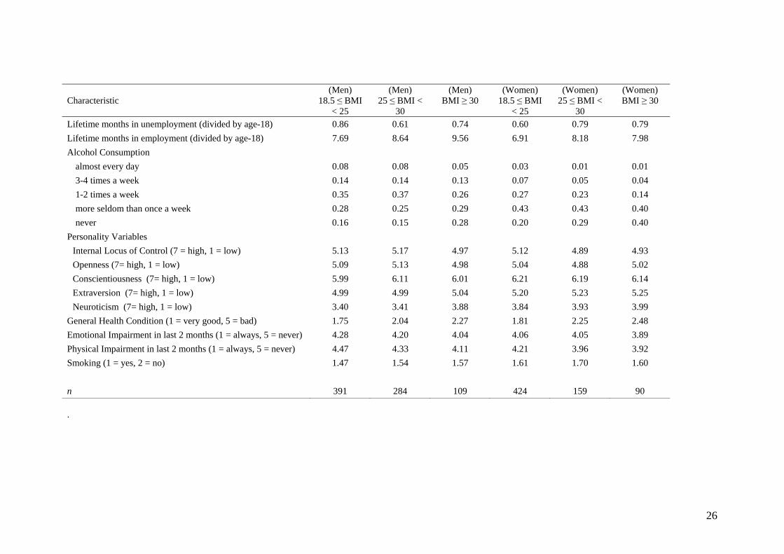
* Table 2 about here *
Table 2 also examines group differences in personality traits and health. With
regards to personality characteristics, it can be seen that obese men and women have
lower values for their internal locus of control, which suggest that obese persons are
more likely to believe that fate or chance primarily determine their life events and
destiny. Another main difference that can be seen is with regards to health, where
obese men and women are more likely than non-obese men and women to have bad
general health and a physical impairment in the last two months.
3. Obesity and labor market outcomes
Active labor market policies in Germany aim to reintegrate unemployed
individuals into the labor market. Active and passive labor market policies have been
reformed substantially between 2003 and 2005 within the ‘Hartz-reforms’, where the
reforms touched the core elements of the labor market, the organizational structure of
the labor offices as well as the pension system. As a general goal, the reforms aimed
at increasing incentives to take up work (see Eichhorst and Zimmermann, 2007, for an
overview). One of the most substantial parts of the welfare reform (Hartz IV) took
5

place in the beginning of 2005.4 Much research has focused on examining the effects
of different types of training programs – affecting the labor supply side of the market
– on individual employment outcomes.5 However, considerable less attention has
been placed on the demand side of the market. How do employers decide whom to
hire from a pool of unemployed workers? What factors affect how long they are hired
for?
Given the tendency for obesity to be strongly associated with low
socioeconomic status (e.g., Brunello et al., 2009) and the interest in helping the
unemployed transition from unemployment to employment, in addition to job training
programs that aim in helping individuals improve their human capital, considerable
attention has been put on identifying potential barriers to employment on the supply
side. For example, Danziger et al. (2000), Jayakody and Stauffer (2000), and
Corcoran et al. (2004) examine a variety of mental and physical health barriers that
reduce the probability of labor market success. Considerable less research has been
devoted to another potential barrier to employment - obesity. With the exception of
Cawley and Danziger (2005), we are not aware of any other study that focuses on
obesity as a barrier in helping welfare recipients transition from welfare-to-work.
A correlation between body weight and labor market outcomes could arise for
several reasons. As Cawley (2004) notes, the first explanation is that obesity lowers
wages. This explanation consists of both demand and supply side factors. On the
supply side, obesity may impair one’s ability to work through having poor health or
low self-esteem. In addition, obese persons may be less motivated to invest in their
own human capital. For example, obese persons might place a higher premium on
present consumption and satisfaction and be less concerned about longer term health
consequences. They could therefore also plausibly be less likely to engage in
activities like training, which only have payoffs in the more distant future. On the
demand side, there could be discrimination by employers. This might arise from
4 Jacobi and Kluve (2007) provide a detailed survey of the reform package. Under Hartz IV, for the first time, extensive efforts were made to reintegrate welfare recipients into the labor market. Recipients were required to participate in welfare to work programs, and were subject to sanctions for non-compliance or rejection of suitable job offers. In these respects, the Hartz IV reform shares many similarities with the 1996 Personal Responsibility and Work Opportunity Act (PRWORA) in the U.S., which required most welfare recipients to seek employment. 5 For example, Card et al. (2009) perform a meta-analysis of 97 studies conducted between 1995 and 2007 and find that in general, job search assistance programs have relatively favorable short-run impacts, whereas classroom and on-the-job training programs tend to show better outcomes in the medium-run than the short-run.
6

employers being prejudiced against the obese and having a distaste for working or
dealing with them; from employers stereotyping obese workers and thinking that they
are less productive; or having a higher uncertainty or a lack of knowledge about the
productivity of obese workers. The second explanation is that low wages or
unemployment help cause obesity (i.e., the case of reverse causality). This would be
true if poorer people consume cheaper food high in fat content. The third explanation
is that there could be unobserved variables that are correlated with both obesity and
employment (e.g., individual time preference).
There is a small literature in economics that examines the effects of obesity on
employment and wages (e.g., Register and Williams, 1990; Loh, 1993; Sargent and
Blanchflower, 1994; Pagan and Davila, 1997; Harper, 2000). More recent studies in
this literature have paid more attention to controlling for the possible endogeneity of
obesity with employment and wages using instrumental variable (IV) approaches
(e.g., Cawley, 2004; Cawley et al., 2005; Brunello and D’Hombres, 2007; Morris,
2007; Lindeboom et al., 2010). In addition, lagged body weight has been used in
place of current body weight in order to avoid the influence of wages on
contemporaneous weight (e.g., Conley and Glauber, 2006). Fixed effects models have
also been used to eliminate the influence of time-invariant unobserved heterogeneity
on weight and wages (e.g., Averett and Korenman, 1996). These studies generally
tend to find that obese women earn less than healthy-weight women.
As Garcia and Quintana-Domeque (2006), Cawley (2007) and Lindeboom et
al. (2010) note, however, establishing convincing causal effects of obesity is not easy.
For example, it appears that a plausible instrument for obesity is to use the BMI of a
family member. But there is a possibility that a substantial part of the genes
responsible for obesity are also responsible for other factors that affect labor market
success.
Experiments provide one convincing way of estimating the causal effects of
obesity. Adopting a field experiment approach, Rooth (2009) identifies differences in
labor market outcomes due to obesity that can be interpreted as causal. He achieves
this by weight manipulation of facial photographs attached to job applications. The
basis for conducting such an experiment comes from lab settings in which
psychologists and sociologists have been documenting systematic differential
treatment by employers against obese applicants (e.g., see Roehling, 1999). In his
experiment, Rooth (2009) sent two equivalent applications to advertised job openings
7

with the only difference being that one has a picture of a person with normal weight
and the other has a digitally modified picture to make the same person look obese. A
key advantage of this approach is that it helps ensure that other supply side
characteristics of the job applicant are held constant. However, a disadvantage of field
experiments of this nature is that it focuses on callback rates or offers for an
interview, and not the actual event of being offered a job.6
Given the difficulties in plausibly estimating a causal effect of obesity when
an experimental design is not feasible, as an alternative, it is possible to perform an
accounting exercise and simply focus on estimating the magnitude of the raw and
conditional gap in outcomes between obese and non-obese individuals. In this case,
the focus is not on estimating average treatment effects but instead on a more general
issue – estimating the magnitude of any potential discrimination that might lead to
obese job applicants being treated or behaving differently from non-obese applicants.
Here, decomposition approaches can be used to distinguish between explained and
unexplained components of the gap that is observed between obese and non-obese
individuals.
3.1 Discrimination against the obese – a theoretical perspective
Employers might choose not to hire obese persons due to widespread negative
stereotypes that overweight and obese persons are lazy, unmotivated, lacking in self-
discipline, less competent, noncompliant, and sloppy (Puhl and Brownell, 2001). Is
there an economic rational basis for such discrimination?
Statistical discrimination is said to occur when rational decision makers use
aggregate group characteristics to evaluate individuals with whom they interact. As a
result, individuals belonging to different groups may be treated differently even if
they share identical observable characteristics in every other respect. The basic
premise of statistical discrimination is that firms have limited information about the
skills and turnover propensity of applicants, particularly workers with little labor
market history. As such, firms have an incentive to use easily observable group
6 In addition to responding to job vacancies using written job applications, approaches using actual persons who pretend to have similar qualifications except for the variable of interest (race, gender etc.) have also been used. The advantages and disadvantages of these ‘audit tests’ are discussed in more detail in Riach and Rich (2002), who provide a broad survey of such field experiments of discrimination.
8
characteristics to ‘statistically discriminate’ among workers if these characteristics are
correlated with performance (e.g., Altonji and Blank, 1999).
Several theoretical models of statistical discrimination developed in the
economics literature suggest why there could be discrimination by employers against
the obese. In his seminal work on discrimination, Becker (1957) assumes that some
agents have a ‘taste’ for discrimination. Employers taste for discrimination affects
profits through wages and hiring decisions. An implication of Becker’s model is that
preferential hiring occurs – employers are less likely to hire obese workers of
identical productivity.
Alternatively, information problems are fundamentally important in labor
markets. When firms are uncertain about the true abilities and effort levels of
prospective employees, it is common to turn to group identification as a signal of
underlying productivity. The statistical discrimination model in Aigner and Cain
(1977) highlights the type of discrimination that can occur when there is a higher
uncertainty about the productivity of obese workers. The model posits two groups of
individuals with known normal distributions of productivity. Although the population
distribution of productivities is known, the actual productivity of any given worker is
unobservable to firms. Instead, firms only observe a noisy signal of productivity,
s μ ε= + where ε is 2(0, )N εσ . Assuming that the signal is noisier for the obese
than the non-obese, and that firms are risk-averse, Aigner and Cain (1977) show that
the group with a noisier signal will receive lower average wages. This is because with
risk aversion, wages depend not only on the conditional expectation of productivity
but also on the conditional variance of productivity. As a result, hiring rates are
different across groups even though productivity might be the same.
Theoretical models of discrimination attempt to rationalize discrimination.
However, one must also be willing to concede that economic theory cannot fully
explain the long run existence of discrimination. As Arrow (1998) notes, “[i]t is
natural to suppose that economic analysis can cast light on the economic effects of
discrimination. But can a phenomenon whose manifestations are everywhere in the
social world really be understood, even in only one aspect, by the tools of a single
discipline?” (p. 91). Darity and Mason (1998) also cast a negative light on the ability
of economic theory to account for discrimination: “Since Becker's work, orthodox
microeconomics has been massaged in various ways to produce stories of how
9
discrimination might sustain itself against pressures of the competitive market. The
tacit assumption of these approaches has been to find a way in which discrimination
can increase business profits, or to identify conditions where choosing not to
discriminate might reduce profits” (p. 82).
3.2 Discrimination against the obese – a practical perspective
In this section, we turn to factors that are outside the scope of economic theory
that might help account for discrimination against the obese. Some empirical evidence
in the literature suggests that there might be logical reasons why employers choose
not to employ the obese. Finkelstein et al. (2005) report that obesity results in
significant increases in medical expenditures and absenteeism among full-time
employees. They estimate that the costs of obesity (excluding overweight persons) at
a firm with 1000 employees are approximately US$285,000 per year. Cawley et al.
(2007) found that obese women were 61 percent more likely to miss work time,
compared to women of healthy weight. For morbidly obese women (BMI 40 or
higher), the figure rose to 118 percent. For women, obesity was linked to absenteeism
across all occupational categories. For men, the relationship varied by occupation. For
example, the likelihood of missed work time among men in professional and sales
occupations increased along with weight category. In other occupations – including
managers, office workers, and equipment operators – the risk of missed work time
increased only for morbidly obese men. Taken as a whole, Cawley et al. (2007) found
that obesity and morbid obesity was associated with increased rates of work
absenteeism, with an estimated cost of $4.3 billion (2004 dollars) in the US.
However, the results of these studies need to be interpreted carefully. Due to
weight discrimination in health care, overweight patients might be reluctant to seek
medical care, be more likely to cancel or delay medical appointments, or put off
important preventative health care services. Viewed in this light, higher absenteeism
amongst the obese might be the result of discrimination and should not be used to
justify discrimination. In section 5, we test to see if health is an important channel by
which the effects of obesity operate. We do so by estimating the obesity gap with and
without health variables included. If health is an important mediating variable, we
expect to see any gap between obese and non-obese persons to become smaller when
health variables are controlled for.
10
4. Methodology
This paper uses a pooled linear decomposition approach to estimate the gap in
labor market outcomes between obese and healthy weight persons, as well as between
overweight and healthy weight persons. As we explain below, the approach we use is
closely related to the estimation of average treatment effects. The main difference is
that the assumptions we invoke using the decomposition approach are weaker than the
assumptions underlying the estimation of causal effects.
4.1 Linear decomposition
A common approach employed in the literature to distinguish between
explained and unexplained components is to perform a linear decomposition, based on
the seminal papers of Blinder (1973) and Oaxaca (1973). In the standard Blinder-
Oaxaca (BO) decomposition, separate regressions are estimated for group A
( i A iY X iβ ε= + ) and for group B ( i B iY X iβ ε= + ), where X are individual level
characteristics that help explain differences in Y. The average gap in outcomes
( A BY Y− ) can be expressed as the sum of two components:
( ) ( )A A B A B BX Xβ β− + − Xβ . The first part is attributed to differences in average
characteristics between the two groups. The second part is due to differences in
average returns to the individual characteristics, which may reflect discrimination.
A BXβ represents the outcome for group B if they were treated as if they were
members of group A. It also represents the outcome for members of group A, if they
had the average characteristics of members of group B. An equally valid
decomposition is to express the components of the gap as:
( ) ( )B A B A B AX Xβ β− + − Xβ . Many papers acknowledge this by reporting the results
of both decompositions, as well the decompositions from a pooled regression without
group specific intercepts based on a suggestion by Neumark (1988).
It is worth thinking carefully about what various types of BO decompositions
measure precisely. Closely related to the literature on decomposition and the
estimation of the size of unexplained gaps is the literature on treatment effects. When
performing a decomposition, one controls for as many possible relevant covariates as
possible, calling the remaining group difference unexplainable or a gap. Similarly,
when estimating causal effects, one also controls for as many relevant covariates as
11
possible in order to make the treatment and control groups as similar as possible. The
remaining difference between the groups is then referred to as the average treatment
effect. Their close relationship is immediately obvious when one simply substitutes
the term ‘treatment effect’ for the term ‘unexplained gap’ in a regression framework.
Developments in the program evaluation literature have been very useful in
helping clarify different parameters of interest one might be interested in estimating,
and helping spell out what the two equally valid versions of the BO decomposition
accomplish. In the first instance when the average gap is expressed as:
( ) ( )A A B A B BX Xβ β− + − Xβ
, the focus is on members of group A and we consider the
hypothetical situation of what happens if they had the average characteristics of
members of group B. Renaming group A as the treatment group and group B as the
control group, we can see that this decomposition is closely related to the parameter
of interest known as the average treatment on the treated (ATT). On the other hand, in
the opposite case where the focus is on members of group B and we think about what
happens if they had the average characteristics of members of group A, the parameter
being estimated is the average treatment on the untreated (ATUT).
Recently, Elder et al. (2010) suggest that the pooled BO decomposition
without a group-specific indicator should not be used to distinguish between
explained and unexplained gaps. They instead suggest the coefficient on a group
indicator from an OLS regression for obtaining a single measure of the unexplained
gap, and discuss how this coefficient can essentially be viewed as a weighted average
of the two different ways of doing a BO decomposition.7
Estimating gaps using the OLS approach has been applied to the measurement
of union wage premiums (e.g., Lewis, 1986), racial test score gaps (e.g., Fryer and
Levitt, 2004), and racial wage gaps (e.g., Neal and Johnson, 1996). More recently,
Lundborg et al. (2010) adopt this approach in decomposing the wage gap between
obese and non-obese individuals.
7 A parallel discussion of this issue can be found in Angrist and Pischke (2008) when discussing the different causal parameters that matching and OLS estimate. They note that whereas matching uses the distribution of covariates among the treated to weight covariate specific estimates into an estimate of the ATT, regression produces a variance weighted average of these effects. What this translates into is that while the ATT estimate places most weight on covariate cells containing those who are most likely to be treated, regression places most weight on covariate cells where the conditional variance of treatment status is largest, which occurs where there are equal number of treatment and control observations (Angrist and Pischke, 2008, p.76).
12
An important advantage of viewing our problem as a decomposition problem
rather than a treatment effects problem is that we can focus on the relative importance
of different sets of variables in explaining the observed gap. This can be accomplished
by estimating various OLS models using different combinations of characteristics. On
the other hand, a treatment effects approach would focus on providing a single ‘best’
estimate of the impact of obesity. Importantly, the decomposition approach also does
not require us to make the conditional independence assumption (CIA) underlying
regression or matching estimators that attempt to measure causal effects.8
In our paper, we therefore mainly focus on applying the pooled regression
decomposition approach in order to determine the relative importance of education,
demographic characteristics, psychological factors and health in explaining the
obesity gap among unemployed Germans. Since previous studies have sometimes
observed differences in the effect of body size on the wages of men and women (e.g.,
Averett and Korenman, 1999; Baum and Ford, 2004; Cawley, 2004), we provide
estimates separately for men and women. In addition to estimating gaps between the
obese (BMI ≥ 30) and persons of healthy weight (18.5 ≤ BMI < 25), we also conduct
similar decomposition exercises for comparing persons who are overweight (25 ≤
BMI < 30) with persons of healthy weight.
4.2 Matching
An alternative approach we adopt to estimate the gap in labor market
outcomes between obese and non-obese persons is to use an approach from the
treatment effects literature – matching. Utilizing the matching estimator as a tool to
perform decompositions instead of estimating average treatment effects is similar in
spirit to the papers by Nopo (2008) and Frölich (2007). Unlike in the standard
application of matching in the evaluation literature, when matching is used to perform
a decomposition, it is not necessary that the CIA holds. Any observable that is not
measured simply falls into the residual term.
In this paper, we report our matching estimates based on kernel matching. One
major advantage of kernel matching is the lower variance which is achieved because
more information is used for constructing counterfactual outcomes. This could be 8 This assumption states that conditional on some set of covariates, the potential outcomes for the obese and non-obese are independent of their group status. In practice, unless a rich set of covariates are available that are related to both labor market outcomes and obesity, it can be difficult to fulfil this assumption.
13

important as our groups of obese and non-obese persons are rather small. An
additional advantage of kernel matching comes from the results of Heckman,
Ichimura, and Todd (1998) who derive the asymptotic distribution of these estimators
and show that bootstrapping is valid to draw inference for this matching method. This
allows us to circumvent the issues raised by Abadie and Imbens (2008), pointing out
that bootstrap methods are invalid for nearest neighbor matching.
Before applying kernel matching, assumptions have to be made regarding the
choice of the kernel function and the bandwidth parameter h. The choice of the kernel
appears to be relatively less important in practice. What is seen as more important is
the choice of the bandwidth parameter h where a trade-off between a small variance
and an unbiased estimate of the true density function arises (see the discussion in
Caliendo and Kopeinig, 2008). We test the sensitivity of the results with respect to
different bandwidth choices.
We provide matching estimates as a robustness check for several reasons. In
addition to estimating a different parameter, a semi-parametric matching approach
differs from the parametric BO decomposition approach in two other aspects. First,
the regression function is no longer specified as linear. Second, the adjusted mean
labor market outcome is simulated only for the common support subpopulation. While
this latter issue is largely recognized in the program evaluation literature, it has until
recently not received much attention in decomposition analysis. For example, by not
considering the common support restriction, the BO decomposition is implicitly based
on linear extrapolation and an ‘out-of-support assumption’. Put another way, it
becomes necessary to assume that the linear estimators of the outcomes are also valid
out of the support region of individual characteristics for which they were estimated.
5. Results
We examine the gap between overweight and healthy weight persons, and the
gap between obese and healthy weight persons on three sets of outcomes variables.
The first set relates to the job search process of the unemployed individuals in wave 1
where we observe: (i) the reservation wage and (ii) the search intensity (measured as
the number of job applications). As we observe these outcomes only for individuals
still unemployed and actively searching for work in wave 1, the sample size for these
outcomes is smaller than for the second set of outcomes which relate to participation
in ALMP programs. Here, we distinguish between three outcome variables. The first
14

outcome is participation in any ALMP program within the period of registering
oneself as unemployed and the wave 2 interview. To determine if there are differences
with respect to participation in human-capital enhancing training programs, we
consider participation in training programs as a second outcome variable. Finally, to
test whether there are timing differences in the participation patterns for obese and
non-obese individuals, we also consider participation in the first six months after
registering oneself as unemployed (‘early participation’) as an outcome variable. The
third set of outcomes is from wave 2 and includes the employment status and the
realized wage for those who have a job. We employ OLS models for all outcomes
except for cases where the outcome is binary. For models with binary outcomes such
as employment or participation in ALMP/training programs, we employ probit
models and report marginal effects at the mean values of the covariates. All
estimations are conducted separately by gender.
Table 3 presents estimates of the gap in outcomes between overweight and
healthy weight men. The column labelled ‘raw gap’ is the unadjusted mean difference
in outcomes between the two groups, where it can be seen that significant differences
exist for log reservation wages in wave 1 and employment status in wave 2. This
implies that overweight men are likely to have higher reservation wages than healthy
weight men, and are also more likely to be employed in wave 2. Columns (1) to (4)
each control for different sets of characteristics in order to determine how each of the
characteristics affect the obesity gap. Column (5) includes education, socio-
demographic and personality variables in a single regression. Column (6) includes all
the characteristics in column (5) with the further addition of health variables. The
employment history variables in the ‘other demographics’ category are useful in
trying to control for the labor supply of individuals in the two weight categories in
each of our pairwise comparisons in our regression models. This way, any observed
gap in employment and wage outcomes is more likely to be due to labor demand as
opposed to labor supply. Column (3) in Table 3 shows that for overweight men, these
set of variables are instrumental in reducing the significant raw gap in log reservation
wages. By and large, any gaps found between overweight and health weight men are
eliminated once we control for education, socio-demographic and other
characteristics. For example, in column (6), it can be seen that the raw gap in log
reservation wages is 0.147, but that this is reduced to 0.06 and no longer significant
once we control for our full set of characteristics.
15

* Table 3 about here *
Table 4 presents estimates of the gap in outcomes between obese and healthy
weight men. As with the overweight vs. healthy weight comparison for men, there are
no significant gaps in labor market outcomes once education, socio-demographic and
other characteristics are controlled for.
Although our sample is not representative of the German population as a
whole, our results for overweight and obese men are consistent with the findings in
Cawley et al. (2005) who find no correlation between weight and earnings for
German men using the German Socio-Economic Panel (GSOEP).
* Table 4 about here *
For women, the raw data in Table 5 suggest that overweight women are likely
to have significantly lower reservation wages than healthy weight women, the
opposite of what was found for men. In addition, overweight women are also less
likely than healthy weight women to be employed in wave 2, and also to have lower
log hourly wages in wave 2. However, once the regression models controls for
various sets of relevant characteristics (columns (5) and (6)), the conditional gaps are
no longer found to be significant.
* Table 5 about here *
On the other hand, we find that there are interesting and significant conditional
gaps in search and labor market outcomes for obese women. By wave 2, the model in
column (5) of Table 6, which has controls for education, socio-demographic variables
and personality, reveals that obese women are about 13 percentage points less likely
to be employed relative to healthy weight women; they also earn on average 0.094
less in terms of log hourly wages. The finding that obese women have lower
employment levels is noteworthy and surprising as obese women had relatively lower
reservation wages (-0.139 log points) and made 4.66 more job applications on
average. Obese women also were 12.3 percentage points more likely to participate in
16
a training program and 10.2 percentage points more likely to enrol early in an active
labor market program.9
If the obesity gap is due to health limitations, we expect the obesity coefficient
to become smaller and insignificant once we control for health. When we control for
health (column 6), the conditional gap in search intensity and participation in training
and labor market programs between obese women and healthy weight women remains
statistically significant. In addition, the gap in hourly wages is also still statistically
significant. Although the gap in employment levels is reduced and becomes barely
insignificant (p-value is 0.14), the point estimate of the difference (0.097) remains
quite large.
* Table 6 about here *
When both health and cognitive skills are controlled for, the gaps in the
ALMP variables remain statistically significant but the effects on both employment
and wages lose their significance (results not shown). It is possible that this lack of
statistical significance could be due to small sample size as the point estimates for
employment (-0.055) and log hourly wages (-0.082) are still suggestive that a gap
exists.10 On the other hand, having insignificant gaps are consistent with the findings
in Lundborg et al. (2010) who argue that the negative association between obesity and
earnings runs mainly through obesity’s association with a variety of supply side
characteristics such as cognitive skills, non-cognitive skills and measures of physical
fitness.
As a robustness check, we also use a matching estimator to provide estimates
of the obesity gap. We focus on the results from a propensity score specification that
does not include any potentially endogenous variables such as health (i.e., the
specification in column (5) of the regression models).
9 There were no significant differences in participation in labor market programs in wave 2 (results not shown) so it is unlikely the case that obese women were less likely to be employed in wave 2 because they were still part of a program or undertaking training. 10 The results of the models including cognitive skills (based on the results from three tests on arithmetic and one test on word recall) are not shown in an additional column in Tables 3 to 6 because about 10 percent of our sample did not respond to those questions. As a result, differences in the results between models that did and did not include cognitive skills could reflect either the importance of cognitive skills or be due to non-random selection and a different sample composition. We choose not to estimate all our models on respondents with non-missing values of measures of cognitive skills in order to not further reduce our sample size.
17

Based on kernel matching estimates using the Epanechnikov kernel and
experimenting with alternative bandwidths, there appear to be no significant effects of
obesity on labor market outcomes for men, and only significant results for obese
women. In other words, the matching results for obese women largely reflect the
regression estimates reported in column (5) of Table 6.
* Table 7 about here *
Overall, the matching estimates which do not control for health status suggest
that only obese women suffer some labor market consequences. The finding that the
negative consequences of obesity on labor market outcomes are greater for females
than for males is consistent with the findings from other studies analysing the impact
of obesity on labour market outcomes (e.g., Baum and Ford, 2004; Cawley, 2004;
Harper, 2000; Morris, 2007; Sargent and Blanchflower, 1994).
6. Conclusions
The economics literature has focused on estimating the effects of many
different forms of discrimination. Like other forms of discrimination, weight
discrimination is highly dependent on public perception. It is therefore a useful
exercise to carry out empirical studies on many different subgroups of the population
to measure the full extent of any discrimination that might exist in society. In this
paper, we examined the issue of whether obese job applicants that newly enter
unemployment in Germany have different job search behaviors from non-obese
applicants, whether they participate at the same rate in ALMP programs and whether
they are regarded differently by employers. The thought experiment was to hold a
‘beauty contest’ where employers choose whom to hire first from a line up of
unemployed persons. Unlike other observational studies which are generally based on
obese and non-obese individuals who might already be at different points in the job
ladder (e.g., household surveys), in this case, individuals all start from the same point
– they are newly unemployed. In the sense that we are trying to create a hypothetical
experiment whereby individuals newly entering unemployment are assigned to
different weight groups, our study design might be viewed as being somewhere in-
between an experimental study and a standard observational study.
18
Our results suggest that no discrimination occurs for overweight males and
females. Obese men also do not appear to suffer any forms of discrimination. The
only group we find in our data experiencing any possible form of labor market
discrimination is obese women. Compared to healthy weight women, obese women
made more job applications and engaged more in job training programs. At the same
time we find some indications that they experienced worse (or at best similar)
employment outcomes than healthy weight women. One possible interpretation of
these results is that obese women need to search harder in order to achieve similar
employment outcomes as healthy weight women. Obese women who found a job also
had significantly lower wages than healthy weight women even after controlling for
an extensive set of personal characteristics. Although this might partly be an empirical
realization of the fact that obese women were willing to accept lower wages to begin
with, it could also reflect discrimination on the part of employers.
Our data do not allow us to disentangle whether health problems amongst the
obese might be the result of past discrimination, or whether obesity causes health
problems. Further research on understanding the interaction between obesity, health
and labor market outcomes will be useful.
19

References Abadie, A. and G. Imbens. (2008). On the failure of the bootstrap for matching
estimators. Econometrica 76: 1537–1557. Aigner, D. and G. Cain. (1977). Statistical theories of discrimination in labor markets.
Industrial and Labor Relations Review 30: 175–187. Altonji, J. and R. Blank. (1999). Race and gender in the labor market. In Ashenfelter
and D. Card (Eds.), Handbook of Labor Economics, Volume 3C: 3143–3259. Amsterdam: North-Holland.
Andreyeva T, R. Puhl and K. Brownell. (2008). Changes in perceived weight
discrimination among Americans: 1995–1996 through 2004–2006. Obesity 16: 1129–1134.
Angrist, J. and J. Pischke. (2008). Mostly Harmless Econometrics: An Empiricist's
Companion. New Jersey: Princeton University Press. Averett, S. and S. Korenman. (1996). The economic reality of the beauty myth.
Journal of Human Resources 31:304– 330. Averett, S. and S. Korenman (1999). Black-white differences in social and economic
consequences of obesity. International Journal of Obesity 23: 166–173. Baum, C. and W. Ford. (2004). The wage effects of obesity: a longitudinal study.
Health Economics 13: 885–899. Becker, G. (1957). The Economics of Discrimination. Chicago: University of Chicago
Press. Berghöfer, A., T. Pischon, T. Reinhold, C. Apovian, A. Sharma and S. Willich.
(2008). Obesity prevalence from a European perspective: a systematic review. BMC Public Health 8: 200 (doi:10.1186/1471-2458-8-200).
Blinder, A. (1973). Wage discrimination: Reduced form and structural estimates.
Journal of Human Resources 8: 436–455. Brunello, G. and B. D’Hombres. (2007). Does body weight affect wages? Evidence
from Europe, Economics and Human Biology 5: 1-19. Brunello, G., P. Michaud and A. Sanz-de-Galdeano. (2009). The rise of obesity in
Europe: an economic perspective, Economic Policy 57: 553-596. Burkhauser, R. and J. Cawley. (2008). Beyond BMI: the value of more accurate
measures of fatness and obesity in social science research. Journal of Health Economics 27: 519–529.
Caliendo, M., A. Falk, L. Kaiser, H. Schneider, A. Uhlendorff, G. Van den Berg and
K. Zimmermann. (2011). The IZA evaluation dataset: towards evidence-based
20

labor policy-making. Discussion Paper 5400, IZA Bonn, forthcoming in International Journal of Manpower.
Caliendo, M. and S. Kopeinig. (2008): Some Practical Guidance for the
Implementation of Propensity Score Matching. Journal of Economic Surveys 22: 31-72.
Card, D. J. Kluve and A. Weber. (2009). Active labor market policy evaluations: a
meta-analysis. IZA Working Paper No. 4002. Cawley, J. (2004). The impact of obesity on wages. Journal of Human Resources 39:
452–474. Cawley, J. (2007). The labor market impacts of obesity, in Obesity, Business, and
Public Policy, Z. Acs and A. Lyles (eds.). Northampton: Edward Elgar. Cawley, J. and S. Danziger. (2005). Morbid obesity and the transition from welfare to
work. Journal of Policy Analysis and Management 24: 727-743. Cawley, J., M. Grabka and D. Lilard. (2005). A comparison of the relationship
between obesity and earnings in the US and Germany. Schmollers Jahrbuch 125: 119-129.
Cawley J, J. Rizzo and K. Haas. (2007). Occupation-specific absenteeism costs
associated with obesity and morbid obesity. Journal of Occupational and Environmental Medicine 49:1317-1324.
Corcoran, M., S. Danziger, and R. Tolman. (2004). Employment duration of african-
american and white welfare recipients and the role of persistent health and mental health problems. Women and Health 39: 21–40.
Conley, D. and R. Glauber. (2006). Gender, body mass, and socioeconomic status:
new evidence from the PSID, Advances in Health Economics and Health Services Research 17: 253-275.
Danziger, S., M. Corcoran, C. Heflin, A. Kalil, and J. Levine. (2000). Barriers to the
employment of welfare recipients. In R. Cherry and W. Rodgers (Eds.), Prosperity for All? The Economic Boom and African-Americans, pp. 239272. New York: Russell Sage Foundation.
Eichhorst, W., and K. Zimmermann. (2007): “And then there were four...how many
(and which) measures of active labor market policy do we still need?” Applied Economics Quarterly 53: 243–272.
Finkelstein E, C. Fiebelkorn and G. Wang. (2005). The costs of obesity among full-
time employees. American Journal of Health Promotion 20: 45-51. Flegal K., M. Carroll, C. Ogden and C. Johnson. (2002). Prevalence and trends in
obesity among U.S. adults, 1999–2000. Journal of the American Medical Association 288: 1723-1727.
21
Flegal, K., M. Carroll, C. Ogden and L. Curtin. (2010). Prevalence and trends in
obesity among US adults, 1999-2008. Journal of the American Medical Association 303: 235-241.
Frölich, M. (2007). Propensity score matching without conditional independence
assumption with an application to the gender wage gap in the United Kingdom. Econometrics Journal 10, 359–407.
Fryer, R. and S. Levitt. (2004). Understanding the black-white test score gap in the
first two years of school. Review of Economics and Statistics 86: 447–464. Garcia, J. and C. Quintana-Domeque. (2006). Obesity, employment and wages in
Europe, Advances in Health Economics and Health Services Research 17: 187-217.
Harper, B. (2000). Beauty, stature and the labour market: a British cohort study.
Oxford Bulletin of Economics and Statistics 62: 771–801. Heckman, J., H. Ichimura, and P. Todd. (1998). Matching as an econometric
evaluation estimator. Review of Economic Studies 65: 261–294. Jacobi, L. and J. Kluve. (2007). Before and after the Hartz reforms. the performance
of active labour market policy in Germany. Discussion Paper 41, RWI. Jayakody, R. and D. Stauffer. (2000). Mental health problems among single mothers:
Implications for work and welfare reform. Journal of Social Issues 54: 617–634. Johansson, E., P. Böckerman, U. Kiiskinen and M. Heliövaara. (2009). Obesity and
labour market success in Finland: The difference between having a high BMI and being fat. Economics and Human Biology 7: 36–45.
Lewis, G. (1986). Union Relative Wage Effects: A Survey. Chicago: The University of
Chicago Press. Lindeboom, M., P. Lundborg and B. van der Klaauw. (2010). Assessing the impact of
obesity on labor market outcomes. Economics and Human Biology 8: 309-319. Loh, E. (1993). The economic effects of physical appearance. Social Science
Quarterly 74: 420–438. Lundborg, P., P. Nystedt and D. Rooth. (2010). No country for fat men? Obesity,
earnings, skills, and health among 450,000 Swedish men. IZA Working Paper No. 4775.
Morris, S. (2007). The impact of obesity on employment. Labour Economics 14: 413–
433. Neal, D. and W. Johnson. (1996). The role of premarket factors in black-white wage
differences. Journal of Political Economy 104: 869–895.
22

Neumark, D. (1988). Employers discriminatory behaviour and the estimation of wage
discrimination. Journal of Human Resources 23: 812-860. Nopo, H. (2008). Matching as a tool to decompose wage gaps. Review of Economics
and Statistics 90: 290–299. Oaxaca, R. (1973). Male-female wage differentials in urban labor markets.
International Economic Review 14: 693–709. Pagan, J. and A. Davila. (1997). Obesity, occupational attainment and earnings. Social
Science Quarterly 78: 756–770. Puhl R. and K. Brownell. (2001). Bias, discrimination, and obesity. Obesity Research
9: 788–905. Register, C. and D. Williams. (1980). Wage effects of obesity among young workers.
Social Science Quarterly 71: 130–141. Riach, P. and J. Rich. (2002). Field experiments of discrimination in the market place.
Economic Journal 112, F480-F518. Roehling, M. (1999). Weight-based discrimination in employment: psychological and
legal aspects. Personnel Psychology 52: 969-1016. Roehling M., P. Roehling and S. Pichler. (2007). The relationship between body
weight and perceived weight-related employment discrimination: the role of sex and race. Journal of Vocational Behavior 71: 300–318.
Roehling M., S. Pilcher, F. Oswald and T. Bruce. (2008). The effects of weight bias
on job-related outcomes: a meta-analysis of experimental studies. Academy of Management Annual Meeting, Anahiem, CA.
Rooth, D. (2009). Obesity, attractiveness and differential treatment in hiring: a field
experiment. Journal of Human Resources 44: 710-735. Sargent, J. and D. Blanchflower. (1994). Obesity and stature in adolescence and
earnings in young adulthood: Analysis of a british birth cohort. Archives of Pediatrics and Adolescent Medicine 148: 681–687.
23

24
Table 1: Sample Sizes Full Sample Searching for Job in Wave 1 Men Women Men Women 18.5 ≤ BMI < 25 391 424 192 272 25 ≤ BMI < 30 284 159 153 107 BMI ≥ 30 109 90 56 59 Total 784 673 401 438 Note: People with a BMI smaller than 18.5 are excluded. We also exclude individuals with missing values in key regressors.

Table 2: Socio-Demographic Characteristics by BMI Group
Characteristic (Men)
18.5 ≤ BMI < 25
(Men) 25 ≤ BMI <
30
(Men) BMI ≥ 30
(Women) 18.5 ≤ BMI
< 25
(Women) 25 ≤ BMI <
30
(Women) BMI ≥ 30
West Germany 0.68 0.75 0.76 0.72 0.73 0.63 German citizenship 0.96 0.95 0.94 0.93 0.96 0.96 Migration background 0.13 0.14 0.13 0.17 0.14 0.12 Age 31.07 36.32 38.28 35.70 38.14 40.92 Married (or cohabiting) 0.21 0.36 0.44 0.43 0.57 0.54
One child 0.17 0.13 0.17 0.22 0.19 0.23 Two (or more) children 0.10 0.14 0.14 0.18 0.21 0.10
Unemplomyent benefit recipient (yes) 0.74 0.79 0.80 0.71 0.78 0.70 Level of UB (missing=0) 453.79 617.63 661.60 391.10 435.21 386.06 School leaving degree (Reference = none)
Lower secondary school 0.28 0.28 0.49 0.17 0.21 0.30 Middle secondary school 0.36 0.40 0.28 0.34 0.47 0.50 Specialized upper secondary school 0.33 0.29 0.22 0.48 0.29 0.18
Vocational Training (Reference = none) Internal or external professional training, others 0.63 0.64 0.66 0.61 0.73 0.72 Technical college or university degree 0.24 0.27 0.21 0.32 0.18 0.18
Employment status before unemployment Employed 0.59 0.64 0.65 0.63 0.58 0.66 Subsidized employment 0.04 0.05 0.11 0.03 0.04 0.04 School, apprentice, military, etc. 0.29 0.21 0.14 0.16 0.13 0.12 Maternity leave 0.00 0.00 0.00 0.10 0.13 0.08 Other 0.08 0.10 0.10 0.08 0.11 0.10
(continued)
25
26
Characteristic (Men)
18.5 ≤ BMI < 25
(Men) 25 ≤ BMI <
30
(Men) BMI ≥ 30
(Women) 18.5 ≤ BMI
< 25
(Women) 25 ≤ BMI <
30
(Women) BMI ≥ 30
Lifetime months in unemployment (divided by age-18) 0.86 0.61 0.74 0.60 0.79 0.79 Lifetime months in employment (divided by age-18) 7.69 8.64 9.56 6.91 8.18 7.98 Alcohol Consumption
almost every day 0.08 0.08 0.05 0.03 0.01 0.01 3-4 times a week 0.14 0.14 0.13 0.07 0.05 0.04 1-2 times a week 0.35 0.37 0.26 0.27 0.23 0.14 more seldom than once a week 0.28 0.25 0.29 0.43 0.43 0.40 never 0.16 0.15 0.28 0.20 0.29 0.40
Personality Variables Internal Locus of Control (7 = high, 1 = low) 5.13 5.17 4.97 5.12 4.89 4.93 Openness (7= high, 1 = low) 5.09 5.13 4.98 5.04 4.88 5.02 Conscientiousness (7= high, 1 = low) 5.99 6.11 6.01 6.21 6.19 6.14 Extraversion (7= high, 1 = low) 4.99 4.99 5.04 5.20 5.23 5.25 Neuroticism (7= high, 1 = low) 3.40 3.41 3.88 3.84 3.93 3.99
General Health Condition (1 = very good, 5 = bad) 1.75 2.04 2.27 1.81 2.25 2.48 Emotional Impairment in last 2 months (1 = always, 5 = never) 4.28 4.20 4.04 4.06 4.05 3.89 Physical Impairment in last 2 months (1 = always, 5 = never) 4.47 4.33 4.11 4.21 3.96 3.92 Smoking (1 = yes, 2 = no) 1.47 1.54 1.57 1.61 1.70 1.60 n 391 284 109 424 159 90 .

Table 3: Regression Results of Estimated Gaps: Overweight Men versus Healthy Weight Men
Outcome Variable
Mean for Healthy Weight
Men
Raw gap (1) (2) (3) (4) (5) (6)
Search Variables Log Reservation Wage (a) 1.97 0.147*** 0.115*** 0.048 0.135*** 0.144*** 0.052 0.06 Number of Job Applications (a) 15.29 1.218 0.708 1.994 0.753 1.210 0.936 0.805
Participation in ALMP Variables Any ALMP 0.31 -0.014 -0.017 -0.033 -0.013 -0.017 -0.032 -0.037 Participation in Training 0.16 -0.008 -0.010 -0.007 -0.005 -0.014 -0.007 -0.014 Early Participation in ALMP 0.14 -0.018 -0.017 -0.016 -0.018 -0.022 -0.015 -0.022
Outcome Variables in Wave 2 Employed 0.62 0.066* 0.054 0.029 0.056 0.081** 0.023 0.033 Log Hourly Wages in € (b) 2.15 0.069 0.069 -0.025 0.055 0.063 -0.020 -0.025
Controls for education Controls for other demographics Controls for personality
Controls for health n 675 675 675 675 675 675 675
Note: Significant at the: *10 percent level; **5 percent level; ***1 percent level. For the detailed list of variables in each of the categories (education, other demographics etc.), see Appendix A. We employ OLS models for the reservation wage, the number of job applications and the hourly wage. For the participation in ALMP variables and employment outcomes we use probit models and report marginal effects at the mean values of the covariates. (a) Only observed for those who are unemployed in wave 1 (n = 327). (b) Only observed for those who are employed in wave 2 (n = 400).
27

Table 4: Regression Results of Estimated Gaps: Obese Men versus Healthy Weight Men
Outcome Variable
Mean for Healthy Weight
Men
Raw gap (1) (2) (3) (4) (5) (6)
Search Variables Log Reservation Wage (a) 1.97 0.057 0.064 -0.003 0.104 0.053 0.049 0.063 Number of Job Applications (a) 15.29 0.868 0.494 0.987 0.842 1.306 -0.013 0.479
Participation in ALMP Variables Any ALMP 0.31 0.002 -0.009 -0.002 -0.003 -0.002 -0.005 -0.007 Participation in Training 0.16 0.037 0.022 0.059 0.015 0.027 0.021 0.022 Early Participation in ALMP 0.14 0.009 -0.002 0.036 -0.011 0.011 0.007 0.011
Outcome Variables in Wave 2 Employed 0.62 -0.019 -0.031 -0.120** -0.009 0.03 -0.105 -0.078 Log Hourly Wages in € (b) 2.15 -0.007 0.011 -0.078 0.011 -0.008 -0.043 -0.061
Controls for education Controls for other demographics Controls for personality
Controls for health n 500 500 500 500 500 500 500
Note: Significant at the: *10 percent level; **5 percent level; ***1 percent level. For the detailed list of variables in each of the categories (education, other demographics etc.), see Appendix A. We employ OLS models for the reservation wage, the number of job applications and the hourly wage. For the participation in ALMP variables and employment outcomes we use probit models and report marginal effects at the mean values of the covariates. (a) Only observed for those who are unemployed in wave 1 (n = 232). (b) Only observed for those who are employed in wave 2 (n = 292).
28

Table 5: Regression Results of Estimated Gaps: Overweight Women versus Healthy Weight Women
Outcome Variable
Mean for Healthy Weight Women
Raw gap (1) (2) (3) (4) (5) (6)
Search Variables Log Reservation Wage (a) 1.96 -0.082** -0.019 -0.012 -0.078* -0.062 -0.002 0.01 Number of Job Applications (a) 12.63 0.424 1.011 1.538 -0.047 0.500 1.848 1.871
Participation in ALMP Variables Any ALMP 0.33 0.003 -0.007 -0.019 0.003 0.007 -0.028 -0.033 Participation in Training 0.21 -0.015 -0.024 -0.037 -0.021 -0.032 -0.042 -0.058 Early Participation in ALMP 0.18 -0.022 -0.030 -0.034 -0.026 -0.033 -0.039 -0.051
Outcome Variables in Wave 2 Employed 0.70 -0.107** -0.084* -0.067 -0.095** -0.064 -0.053 -0.015 Log Hourly Wages in € (b) 2.11 -0.093* -0.016 -0.088* -0.083* -0.091* -0.020 -0.021
Controls for education Controls for other demographics Controls for personality
Controls for health n 583 583 583 583 583 583 583
Note: Significant at the: *10 percent level; **5 percent level; ***1 percent level. For the detailed list of variables in each of the categories (education, other demographics etc.), see Appendix A. We employ OLS models for the reservation wage, the number of job applications and the hourly wage. For the participation in ALMP variables and employment outcomes we use probit models and report marginal effects at the mean values of the covariates. (a) Only observed for those who are unemployed in wave 1 (n = 367). (b) Only observed for those who are employed in wave 2 (n = 358).
29

30
Table 6: Regression Results of Estimated Gaps: Obese Women versus Healthy Weight Women
Outcome Variable
Mean for Healthy Weight Women
Raw gap (1) (2) (3) (4) (5) (6)
Search Variables Log Reservation Wage (a) 1.96 -0.214*** -0.148*** -0.163*** -0.212*** -0.187*** -0.139** -0.123** Number of Job Applications (a) 12.63 3.952* 4.179* 4.472** 3.762* 4.350* 4.660** 5.200**
Participation in ALMP Variables Any ALMP 0.33 0.014 0.015 0.044 0.018 0.042 0.05 0.071 Participation in Training 0.21 0.101* 0.09* 0.117* 0.105** 0.101* 0.123** 0.123** Early Participation in ALMP 0.18 0.076 0.066 0.099* 0.079 0.068 0.102* 0.095*
Outcome Variables in Wave 2 Employed 0.70 -0.165*** -0.140** -0.143** -0.156*** -0.116** -0.132** -0.097 Log Hourly Wages in € (b) 2.11 -0.198*** -0.104* -0.167*** -0.204*** -0.164*** -0.094* -0.092*
Controls for education Controls for other demographics Controls for personality
Controls for health n 514 514 514 514 514 514 514
Note: Significant at the: *10 percent level; **5 percent level; ***1 percent level. For the detailed list of variables in each of the categories (education, other demographics etc.), see Appendix A. We employ OLS models for the reservation wage, the number of job applications and the hourly wage. For the participation in ALMP variables and employment outcomes we use probit models and report marginal effects at the mean values of the covariates. (a) Only observed for those who are unemployed in wave 1 (n = 321). (b) Only observed for those who are employed in wave 2 (n = 320).

Table 7: Matching Estimates of the Gap for Men and Women
Outcome Kernel
Matching (bw = 0.02)
Kernel Matching
(bw = 0.06)
Kernel Matching (bw = 0.2)
n for Treated n for Control
a) Overweight Men versus Healthy Weight Men Log Reservation Wage 0.065 0.072 0.085* 146 181 Number of Job Applications 0.821 0.815 1.001 144 180 Any ALMP -0.020 -0.024 -0.023 284 391 Participation in Training -0.001 0.001 -0.003 284 391 Early Participation in ALMP -0.021 -0.018 -0.018 284 391 Employed in Wave 2 -0.001 0.011 0.019 284 391 Log Hourly Wages at Wave 2 -0.026 -0.015 0.008 176 224 b) Obese Men versus Healthy Weight Men Log Reservation Wage 0.017 0.021 -0.001 51 181 Number of Job Applications 1.382 -0.942 1.170 51 180 Any ALMP 0.015 0.018 0.008 109 391 Participation in Training 0.052 0.064 0.056 109 391 Early Participation in ALMP 0.023 0.034 0.028 109 391 Employed in Wave 2 -0.075 -0.078 -0.059 109 391 Log Hourly Wages at Wave 2 -0.111 -0.068 -0.038 68 224 c) Overweight Women versus Healthy Weight Women Log Reservation Wage -0.012 -0.008 -0.023 104 263 Number of Job Applications 0.845 0.935 1.044 103 260 Any ALMP 0.005 -0.005 -0.008 159 424 Participation in Training -0.019 -0.031 -0.028 159 424 Early Participation in ALMP -0.025 -0.033 -0.033 159 424 Employed in Wave 2 -0.069 -0.063 -0.067 159 424 Log Hourly Wages at Wave 2 -0.047 -0.052 -0.067 87 271 d) Obese Women versus Healthy Weight Women Log Reservation Wage -0.140* -0.125 -0.134** 58 256 Number of Job Applications 5.220 4.993 4.719* 58 253 Any ALMP 0.088 0.073 0.055 90 424 Participation in Training 0.159*** 0.145*** 0.130** 90 424 Early Participation in ALMP 0.131** 0.122** 0.109** 90 424 Employed in Wave 2 -0.106 -0.104 -0.118* 90 424 Log Hourly Wages at Wave 2 -0.128* -0.119** -0.126** 49 271 Note: Propensity score models are estimated using the full set of covariates used in Model 5 of the regression results. Matching is performed using the Epanechnikov kernel. Common support is imposed using the min-max criterion. Imposing common support using 5% trimming resulted in similar results and is not shown. Standard errors are based on bootstrapping with 100 replications. Significant at the: *10 percent level; **5 percent level; ***1 percent level.
31

32
Appendix A List of variables used in the regression models in Tables 3-6: Education variables: school leaving degree (none, lower secondary, middle secondary,
specialized secondary), vocational training (professional training, technical college or university degree).
Other demographic variables: West Germany, citizenship, married, number of children (0, 1, 2+),
unemployment benefit recipient, level of benefits, age (17-24, 25-34, 35-44, 45-55), lifetime months in unemployment, lifetime months in employment, month of entry into unemployment, employment status before unemployment (employed, subsidized employment, school/apprentice/military, maternity leave, other), local unemployment rate (<5%, 5-10%, 10-15%,15+%), alcohol consumption (almost every day, 3-4 times a week, 1-2 times a week, more seldom than once a week, never).
Personality variables: openness, conscientiousness, extraversion, neuroticism, internal locus
of control index. Health variables: general health condition (1=very good, 5=bad), emotional
impairment in last 2 months (1=always, 5=never), physical impairment in last 2 months (1=always, 5=never), smoking.


![Adipose Tissue Dysfunction as Determinant of Obesity ......fat accumulation in human is the increased visceral/intra-abdominal fat accumulation, associated with abdominal obesity [23].](https://static.fdocuments.in/doc/165x107/60af1f3f5208f406dd7a5bf3/adipose-tissue-dysfunction-as-determinant-of-obesity-fat-accumulation-in.jpg)