Faster-than-Nyquist System Design for Next Generation ...

Faster-than-Nyquist System Design for Next

Generation Fixed Transmission Networks

by

Mrinmoy Jana

M.Tech, Indian Institute of Technology, Kanpur, India, 2010B.E., Jadavpur University, Kolkata, India, 2008

A THESIS SUBMITTED IN PARTIAL FULFILLMENT OFTHE REQUIREMENTS FOR THE DEGREE OF

DOCTOR OF PHILOSOPHY

in

The Faculty of Graduate and Postdoctoral Studies

(Electrical and Computer Engineering)

THE UNIVERSITY OF BRITISH COLUMBIA

(Vancouver)

November 2019

© Mrinmoy Jana, 2019

The following individuals certify that they have read, and recommend to the Faculty

of Graduate and Postdoctoral Studies for acceptance, the dissertation entitled:

“Faster-than-Nyquist System Design for Next Generation Fixed Trans-

mission Networks”

submitted by Mrinmoy Jana in partial fulfillment of the requirements for the de-

gree of Doctor of Philosophy in Electrical and Computer Engineering.

Examining Committee:

Lutz Lampe, Electrical and Computer Engineering

Supervisor

Sudip Shekhar, Electrical and Computer Engineering

Supervisory Committee Member

Julian Cheng, Electrical and Computer Engineering

Supervisory Committee Member

Cyril Leung, Electrical and Computer Engineering

University Examiner

Eldad Haber, Earth, Ocean and Atmospheric Sciences

University Examiner

ii

Abstract

Monumental growth of traffic load in the communication networks has heavily strained

the existing fixed transmission network infrastructure. Such enormous surge of traffic

warrants enabling higher data rates in these networks, where predominantly optical

fibers and microwave radio links are deployed. With bandwidth becoming an expen-

sive resource, and owing to the practical constraints of the electronic components, em-

ploying high baud rates alone may be insufficient to accomplish such high throughputs

in these optical fiber communication (OFC) and microwave communication (MWC)

systems. Hence, increasing the spectral efficiency (SE) is a key requirement for these

networks.

For this pursuit, this thesis investigates the application of Faster-than-Nyquist

(FTN) signaling in fixed transmission networks, with an objective to achieve high

SE and data rates. FTN is an enabling technology that offers SE improvements by

allowing controlled overlap of the transmitted symbols in time or frequency or both.

OFC and MWC systems are suitable platforms for the introduction of FTN signaling,

since FTN can moderate the need for higher order modulation formats, which are

sensitive to phase noise and fiber nonlinearity. In this thesis, we combine the concept

of FTN signaling with other conventional throughput increasing techniques, such

as polarization multiplexing and multicarrier transmission, to further the data rate

improvements.

However, FTN introduces inter-symbol-interference and/or inter-carrier interfer-

iii

ence. Moreover, integrating FTN signaling with polarization multiplexing and mul-

ticarrier transmission complicates the realistic implementation. OFC and MWC sys-

tems also pose additional practical challenges stemming from the specific commu-

nication channel environments and the transceiver components. If not successfully

mitigated, all of these impairments and non-idealities significantly deteriorate the

performance of the communication links.

In this thesis, we address each of these unique challenges through suitable miti-

gation algorithms, to facilitate an efficient FTN transmission. For this, we present

sophisticated system designs equipped with powerful digital signal processing tools.

We numerically evaluate the performance of our proposed methods by simulating

realistic OFC and MWC systems. The simulation results indicate that our proposed

spectrally efficient designs offer significant performance advantages over existing com-

petitive schemes.

iv

Lay Summary

Fixed transmission networks serve as the backbone for the Internet and the mobile

data traffic. Currently, optical fibers and microwave radio constitute majority of the

communication links in such networks. With bandwidth becoming an increasingly

critical resource, spectrally efficient technologies need to be employed in these net-

works to cope with the skyrocketing traffic demands. Faster-than-Nyquist (FTN)

signaling is one such befitting technique to accomplish this purpose. However, the

benefits of FTN come at the price of introducing interference. Moreover, practical

OFC and MWC systems present unique complications of their own. In this thesis,

we explore the possibility of applying FTN signaling in the next generation fixed

transmission networks. For this, we present powerful signal processing tools to miti-

gate the interference and other practical challenges imposed by the realistic OFC and

MWC systems. The simulation results we provide in this thesis establish substantial

superiority of the proposed schemes over state-of-the-art designs.

v

Preface

This thesis is based on original research that I conducted under the supervision of

Professor Lutz Lampe in the Department of Electrical and Computer Engineering at

the University of British Columbia, Vancouver, Canada.

The co-authors in my publications, Dr. Jeebak Mitra and Dr. Ahmed Medra, from

Huawei Technologies, Kanata, ON, Canada, have assisted me towards the problem

formulation and provided me valuable suggestions to determine the relevance of the

solutions with respect to the practical intricacies of fixed transmission networks.

Below is a list of publications related to the work presented in this thesis. For all

of them, I was responsible for reviewing literature, developing solutions, evaluating

them through simulations, and preparing publication manuscripts. Professor Lutz

Lampe supervised all my work.

Publications Related to Chapter 2

• M. Jana, A. Medra, L. Lampe, J. Mitra, “Pre-Equalized Faster-Than-Nyquist

Transmission”, IEEE Trans. Commun., vol. 65, no. 10, pp. 4406–4418, Oct. 2017.

• M. Jana, A. Medra, L. Lampe, J. Mitra, “Precoded Faster-than-Nyquist Co-

herent Optical Transmission”, in Proc. 42nd European Conf. Opt. Commun.

(ECOC), Dusseldorf, Germany, Sep. 2016.

vi

• M. Jana, J. Mitra, L. Lampe, A. Medra “System and Method for Precoded

Faster-than-Nyquist Signaling”, US Patent 10003390, Date of patent: Jun. 19, 2018.


• M. Jana, L. Lampe, J. Mitra, “Dual-Polarized Faster-Than-Nyquist Trans-

mission Using Higher Order Modulation Schemes”, IEEE Trans. Commun.,

vol. 66, no. 11, pp. 5332–5345, Nov. 2018.

• M. Jana, L. Lampe, J. Mitra, “Interference and Phase Noise Mitigation in a

Dual-Polarized Faster-than-Nyquist Transmission,” Proc. IEEE Int. Workshop

Sig. Proc. Adv. Wireless Commun. (SPAWC), Kalamata, Greece, June 2018.

• M. Jana, J. Mitra, L. Lampe “Methods and Systems for Interference Mitiga-

tion in a Dual-Polarized Communication System”, US Patent 10425256, Date

of patent: Sep. 24, 2019.


• M. Jana, L. Lampe, J. Mitra, “Precoded Time-Frequency-Packed Multicarrier

Faster-than-Nyquist Transmission,” Finalist, Best Student Paper Award,

Proc. IEEE Int. Workshop Sig. Proc. Adv. Wireless Commun. (SPAWC),

Cannes, France, July 2019.

vii


• M. Jana, L. Lampe, J. Mitra, “Interference Cancellation for Time-Frequency

Packed Super-Nyquist WDM Systems”, IEEE Photon. Technol. Lett, vol. 30,

no. 24, pp. 2099–2102, Dec. 2018.


• M. Jana, L. Lampe, J. Mitra, “Spectrally Efficient Time-Frequency Packed

WDM Superchannel Transmission”, to be submitted, 2019.

• M. Jana, J. Mitra, L. Lampe “System and Method for Multichannel Optical

Transmission with Interference Mitigation”, Utility patent application being

drafted, to be submitted, 2019.

• M. Jana, J. Mitra, L. Lampe “System and method for Phase Noise mitigation

in Coherent Optical Transceivers”, Utility patent application being drafted, to

be submitted, 2019.

viii

Table of Contents

Abstract . . . . . . . . . . . . . . . . . . . . . . . . . . . . . . . . . . . . . . iii

Lay Summary . . . . . . . . . . . . . . . . . . . . . . . . . . . . . . . . . . v

Preface . . . . . . . . . . . . . . . . . . . . . . . . . . . . . . . . . . . . . . vi

Table of Contents . . . . . . . . . . . . . . . . . . . . . . . . . . . . . . . . ix

List of Tables . . . . . . . . . . . . . . . . . . . . . . . . . . . . . . . . . . xv

List of Figures . . . . . . . . . . . . . . . . . . . . . . . . . . . . . . . . . . xvi

List of Abbreviations . . . . . . . . . . . . . . . . . . . . . . . . . . . . . . xxi

Notation . . . . . . . . . . . . . . . . . . . . . . . . . . . . . . . . . . . . . xxvi

Acknowledgments . . . . . . . . . . . . . . . . . . . . . . . . . . . . . . . .xxviii

Dedication . . . . . . . . . . . . . . . . . . . . . . . . . . . . . . . . . . . . xxx

1 Introduction . . . . . . . . . . . . . . . . . . . . . . . . . . . . . . . . . 1

1.1 Background & Motivation . . . . . . . . . . . . . . . . . . . . . . . . 1

1.1.1 Why Fixed Transmission Networks? . . . . . . . . . . . . . . 1

1.1.2 Why Faster-than-Nyquist (FTN) Transmission? . . . . . . . 5

1.2 Enabling Technologies . . . . . . . . . . . . . . . . . . . . . . . . . . 6

ix

1.2.1 FTN Signaling . . . . . . . . . . . . . . . . . . . . . . . . . . 7

1.2.2 Time-Frequency Packing . . . . . . . . . . . . . . . . . . . . 7

1.2.3 Polarization Multiplexing . . . . . . . . . . . . . . . . . . . . 8

1.2.4 Higher-order Modulation Schemes . . . . . . . . . . . . . . . 8

1.3 Literature Review . . . . . . . . . . . . . . . . . . . . . . . . . . . . 9

1.3.1 Single Carrier DP FTN OFC Systems . . . . . . . . . . . . . 10

1.3.2 Single Carrier DP FTN MWC Systems . . . . . . . . . . . . 11

1.3.3 Multicarrier DP FTN OFC Systems . . . . . . . . . . . . . . 14

1.4 Contributions of the Thesis . . . . . . . . . . . . . . . . . . . . . . . 15

1.4.1 Single Carrier DP FTN Transmission for OFC . . . . . . . . 16

1.4.2 Single Carrier DP FTN HoM Transmission for MWC . . . . . 17

1.4.3 TFP WDM Superchannel Transmission for OFC . . . . . . . 18

1.5 Organization of the Thesis . . . . . . . . . . . . . . . . . . . . . . . 19

2 FTN Transmission for Single-Carrier OFC Systems . . . . . . . . 21

2.1 Introduction . . . . . . . . . . . . . . . . . . . . . . . . . . . . . . . 21

2.2 System Model . . . . . . . . . . . . . . . . . . . . . . . . . . . . . . 23

2.2.1 Precoded FTN . . . . . . . . . . . . . . . . . . . . . . . . . . 23

2.2.2 Spectral Factorization . . . . . . . . . . . . . . . . . . . . . . 25

2.3 Non-linear Precoding in FTN Systems . . . . . . . . . . . . . . . . . 26

2.3.1 THP-precoded FTN . . . . . . . . . . . . . . . . . . . . . . . 26

2.3.2 Expanded A-priori Demapper (EAD) . . . . . . . . . . . . . 28

2.3.3 Sliding-Window-EAD (SW-EAD) . . . . . . . . . . . . . . . . 31

2.3.4 Precoding-loss for FTN-THP Systems . . . . . . . . . . . . . 32

2.4 Linear Pre-equalization for FTN . . . . . . . . . . . . . . . . . . . . 34

2.5 Numerical Results and Discussion . . . . . . . . . . . . . . . . . . . 38

x

2.5.1 Simulation Setup . . . . . . . . . . . . . . . . . . . . . . . . . 39

2.5.2 Performance of FTN-THP with Proposed Demappers . . . . 40

2.5.3 Computational Complexity Analysis . . . . . . . . . . . . . . 44

2.5.4 Performance of Proposed FTN-LPE . . . . . . . . . . . . . . 45

2.6 Conclusions . . . . . . . . . . . . . . . . . . . . . . . . . . . . . . . . 51

3 FTN Transmission for Single-Carrier MWC Systems . . . . . . . . 52

3.1 Introduction . . . . . . . . . . . . . . . . . . . . . . . . . . . . . . . 52

3.2 System Model . . . . . . . . . . . . . . . . . . . . . . . . . . . . . . 55

3.3 Adaptive DFE with PN Compensation . . . . . . . . . . . . . . . . . 58

3.3.1 Combined Phase Noise Tracking (CPNT) . . . . . . . . . . . 59

3.3.2 Individual Phase Noise Tracking (IPNT) . . . . . . . . . . . . 63

3.4 XPIC with Precoded FTN . . . . . . . . . . . . . . . . . . . . . . . . 66

3.5 Numerical Results and Discussion . . . . . . . . . . . . . . . . . . . 69

3.5.1 Simulation Setup . . . . . . . . . . . . . . . . . . . . . . . . . 69

3.5.2 Performance with DFE-FTN . . . . . . . . . . . . . . . . . . 71

3.5.3 Performance with LPE-FTN . . . . . . . . . . . . . . . . . . 76


3.6 Conclusions . . . . . . . . . . . . . . . . . . . . . . . . . . . . . . . . 82

4 Multicarrier Faster-than-Nyquist Optical Transmission . . . . . . 83

4.1 Introduction . . . . . . . . . . . . . . . . . . . . . . . . . . . . . . . 83

4.2 System Model . . . . . . . . . . . . . . . . . . . . . . . . . . . . . . 84

4.3 Precoding Solutions . . . . . . . . . . . . . . . . . . . . . . . . . . . 86

4.3.1 Joint precoding: 2-D LPE . . . . . . . . . . . . . . . . . . . . 86

4.3.2 Partial Precoding (PP) . . . . . . . . . . . . . . . . . . . . . 89

4.4 Numerical results . . . . . . . . . . . . . . . . . . . . . . . . . . . . . 90

xi

4.4.1 Simulation Parameters . . . . . . . . . . . . . . . . . . . . . . 91

4.4.2 2-D LPE Gains . . . . . . . . . . . . . . . . . . . . . . . . . . 92

4.4.3 Feasible Range for 2-D LPE . . . . . . . . . . . . . . . . . . . 94

4.4.4 PP Gains . . . . . . . . . . . . . . . . . . . . . . . . . . . . . 95

4.4.5 Computational Complexity . . . . . . . . . . . . . . . . . . . 95

4.5 Conclusions . . . . . . . . . . . . . . . . . . . . . . . . . . . . . . . . 96

5 Towards Terabit-per-second Super-Nyquist Systems . . . . . . . . 97

5.1 Introduction . . . . . . . . . . . . . . . . . . . . . . . . . . . . . . . 97

5.2 System model . . . . . . . . . . . . . . . . . . . . . . . . . . . . . . 100

5.3 FP WDM Transmission: ICIC . . . . . . . . . . . . . . . . . . . . . 101

5.3.1 Linear Equalization . . . . . . . . . . . . . . . . . . . . . . . 101

5.3.2 Iterative Equalization: Turbo-PIC . . . . . . . . . . . . . . . 102

5.4 TFP WDM Transmission: ISIC & ICIC . . . . . . . . . . . . . . . . 104

5.5 Results and Discussion . . . . . . . . . . . . . . . . . . . . . . . . . . 104


5.5.2 ISI vs. ICI Trade-off . . . . . . . . . . . . . . . . . . . . . . . 106

5.5.3 LE-ICIC vs Turbo-PIC . . . . . . . . . . . . . . . . . . . . . 107

5.5.4 TFP Gains . . . . . . . . . . . . . . . . . . . . . . . . . . . . 108

5.5.5 Computational Complexity . . . . . . . . . . . . . . . . . . . 111

5.6 Conclusions . . . . . . . . . . . . . . . . . . . . . . . . . . . . . . . . 112

6 Flexible Designs for Spectrally Efficient TFP Superchannels . . . 113

6.1 Introduction . . . . . . . . . . . . . . . . . . . . . . . . . . . . . . . 113

6.2 System Model . . . . . . . . . . . . . . . . . . . . . . . . . . . . . . 116

6.3 Interference Channel Estimation and CPNE . . . . . . . . . . . . . . 118

6.3.1 DSP Modules . . . . . . . . . . . . . . . . . . . . . . . . . . . 119

xii

6.3.2 LMS Update Equations . . . . . . . . . . . . . . . . . . . . . 119

6.3.3 Data-aided and Decisions-directed Adaptation . . . . . . . . 121

6.4 Iterative PN Estimation (IPNE) . . . . . . . . . . . . . . . . . . . . 122

6.4.1 LIPNE . . . . . . . . . . . . . . . . . . . . . . . . . . . . . . 123

6.4.2 FGIPNE . . . . . . . . . . . . . . . . . . . . . . . . . . . . . 123

6.5 Interference Cancellation . . . . . . . . . . . . . . . . . . . . . . . . 124

6.5.1 Basic Turbo ISIC-ICIC Structure . . . . . . . . . . . . . . . . 124

6.5.2 ICIC Scheduling: SPCIC . . . . . . . . . . . . . . . . . . . . 126

6.6 Numerical Results . . . . . . . . . . . . . . . . . . . . . . . . . . . . 128


6.6.2 Interference Channel Estimation and Cancellation Gains . . . 130

6.6.3 Tolerance to Cascaded ROADMs . . . . . . . . . . . . . . . . 134

6.6.4 Tolerance to Laser Linewidth . . . . . . . . . . . . . . . . . . 137


6.7 Conclusion . . . . . . . . . . . . . . . . . . . . . . . . . . . . . . . . 139

7 Concluding Remarks & Future Directions . . . . . . . . . . . . . . . 141

7.1 Summary and Conclusions . . . . . . . . . . . . . . . . . . . . . . . 141

7.2 Future Work . . . . . . . . . . . . . . . . . . . . . . . . . . . . . . . 144

7.2.1 FTN and Probabilistic Shaping . . . . . . . . . . . . . . . . . 144

7.2.2 Fiber Nonlinearity . . . . . . . . . . . . . . . . . . . . . . . . 145

7.2.3 Additional Device Non-idealities and Impairments . . . . . . 145

Bibliography . . . . . . . . . . . . . . . . . . . . . . . . . . . . . . . . . . . 146

Appendices . . . . . . . . . . . . . . . . . . . . . . . . . . . . . . . . . . . . 163

xiii

Appendix A Proofs and Derivations for Chapter 2 . . . . . . . . . . . 164

A.1 Proof of Proposition 2.1 . . . . . . . . . . . . . . . . . . . . . . . . . 164

A.2 Proof of Proposition 2.2 . . . . . . . . . . . . . . . . . . . . . . . . . 165

A.3 PSD And Average Transmit Power with Precoding . . . . . . . . . . 166

Appendix B Proofs and Derivations for Chapter 3 . . . . . . . . . . . 170

B.1 LMS Update Equations . . . . . . . . . . . . . . . . . . . . . . . . . 170

B.1.1 Proof of Lemma 3.1 . . . . . . . . . . . . . . . . . . . . . . . 170

B.1.2 Proof of Lemma 3.2 . . . . . . . . . . . . . . . . . . . . . . . 172

B.2 LPE-FFF and LPE-FBF Computations . . . . . . . . . . . . . . . . 173

Appendix C Proofs and Derivations for Chapter 4 . . . . . . . . . . . 174

C.1 Proof of Proposition 4.1 . . . . . . . . . . . . . . . . . . . . . . . . . 174

C.2 Proof of Proposition 4.2 . . . . . . . . . . . . . . . . . . . . . . . . . 175

C.3 2-D LPE PMD Equalizer LMS Algorithm . . . . . . . . . . . . . . . 175

Appendix D Proofs and Derivations for Chapter 5 . . . . . . . . . . . 177

D.1 Proof of Lemma 5.1 . . . . . . . . . . . . . . . . . . . . . . . . . . . 177

D.2 Proof of Lemma 5.2 . . . . . . . . . . . . . . . . . . . . . . . . . . . 177

Appendix E Proofs and Derivations for Chapter 6 . . . . . . . . . . . 179

E.1 FGIPNE Metrics Computation . . . . . . . . . . . . . . . . . . . . . 179

xiv

List of Tables

2.1 Computational complexities of the THP-demappers for each bit and

iteration. . . . . . . . . . . . . . . . . . . . . . . . . . . . . . . . . . . 44

2.2 Complexity comparison of the demappers per bit per iteration: QPSK,

β = 0.3,τ = 0.84 and τ = 0.8. . . . . . . . . . . . . . . . . . . . . . . 44

3.1 Computational Complexities: CPNT vs. IPNT . . . . . . . . . . . . . 81

4.1 Complexity, memory and latency, per codeword . . . . . . . . . . . . 95

5.1 Complexity, memory and latency per codeword . . . . . . . . . . . . 111

6.1 Simulation parameters . . . . . . . . . . . . . . . . . . . . . . . . . . 129

6.2 Computational Complexity. . . . . . . . . . . . . . . . . . . . . . . . 138

xv

List of Figures

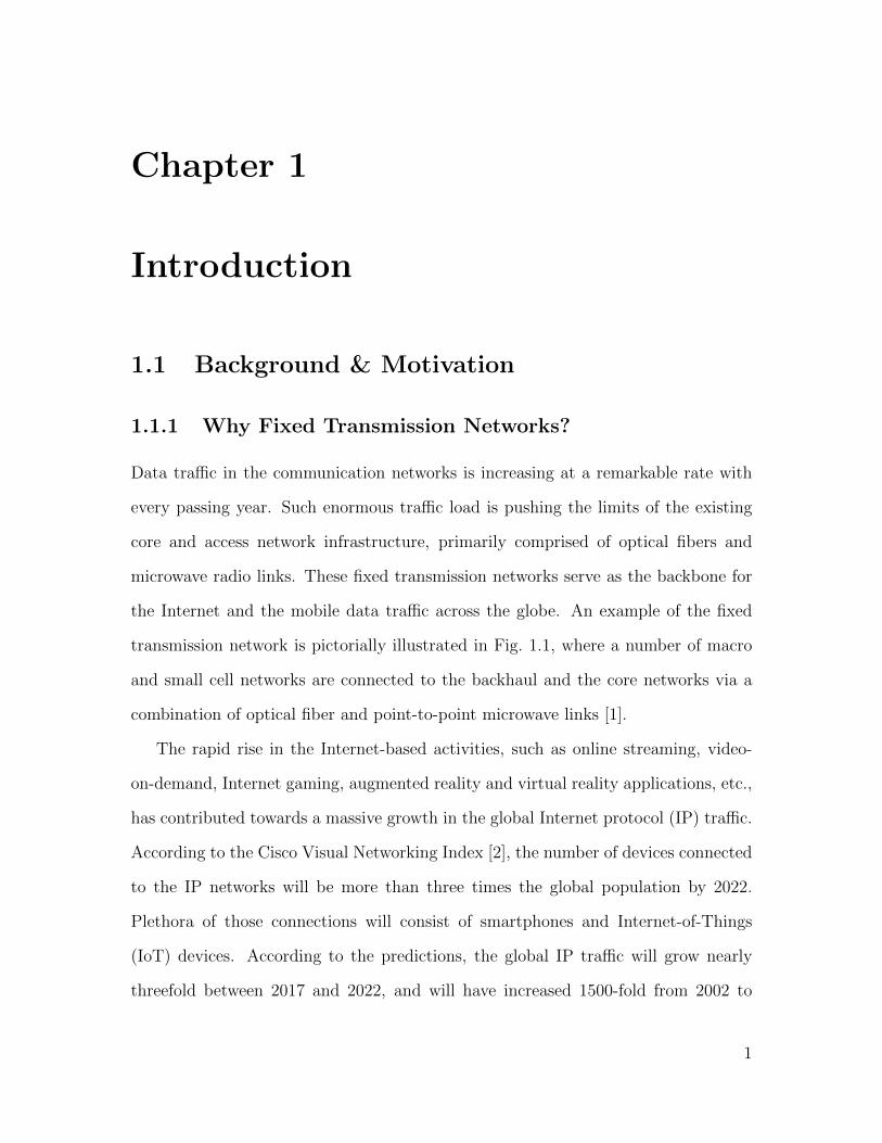
1.1 Example of a typical backhaul and core network infrastructure. The

schematics of the figure are adopted from [1]. . . . . . . . . . . . . . . 2

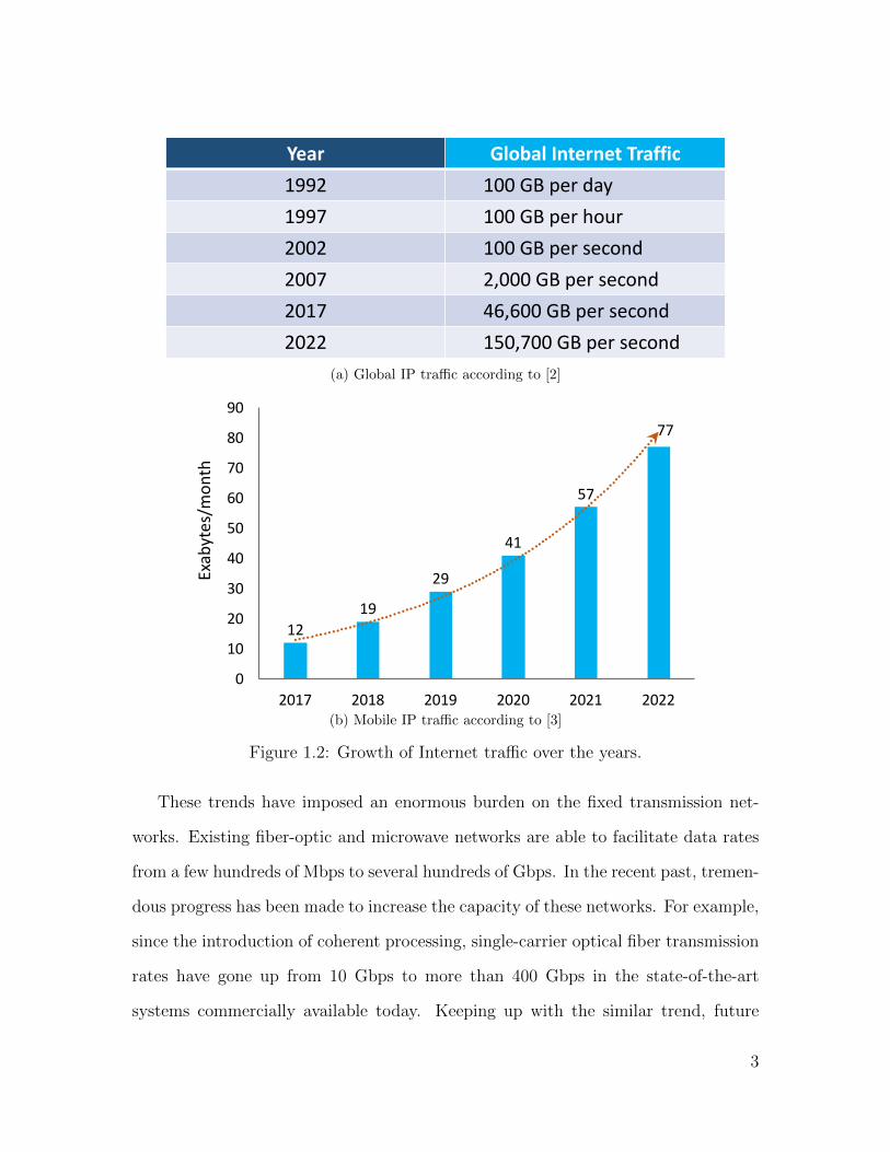
1.2 Growth of Internet traffic over the years. . . . . . . . . . . . . . . . . 3

1.3 Predictions for microwave backhaul capacity per site, according to [4]. 4

1.4 Summary of thesis contributions: FTN for OFC and MWC fixed trans-

mission networks. . . . . . . . . . . . . . . . . . . . . . . . . . . . . . 16

2.1 Baseband system model for a pre-equalized FTN transmission where

the shaded blocks at the transmitter and the receiver represent the

proposed FTN pre-equalizer and symbol demappers respectively. . . . 23

2.2 FTN pre-equalization with THP and the modulo-equivalent linear

structure. . . . . . . . . . . . . . . . . . . . . . . . . . . . . . . . . . 26

2.3 Linear pre-equalization of FTN ISI. . . . . . . . . . . . . . . . . . . . 34

2.4 Block diagram of the precoded FTN dual-polarized coherent optical

simulation setup where the shaded blocks at the transmitter and the

receiver represent the proposed THP/LPE pre-equalizer and symbol

demappers respectively. . . . . . . . . . . . . . . . . . . . . . . . . . . 38

2.5 BER vs. OSNR for FTN-THP with different demappers, illustrating

the performance of the proposed EAD. QPSK, β = 0.3, τ = 0.85 and

0.8. . . . . . . . . . . . . . . . . . . . . . . . . . . . . . . . . . . . . . 40

xvi

2.6 Auto-correlation of the expanded constellation symbols v for β = 0.3

and τ = 0.8. . . . . . . . . . . . . . . . . . . . . . . . . . . . . . . . . 41

2.7 BER vs. OSNR for FTN-THP with different demappers, illustrating

the performance gains with the proposed SW-EAD over EAD. QPSK,

β = 0.3 and τ = 0.8. . . . . . . . . . . . . . . . . . . . . . . . . . . . 42

2.8 SNR vs. τ in a QPSK FTN-THP system for varying β. . . . . . . . . 43

2.9 BER vs. OSNR for FTN with LPE precoding. QPSK with τ = 0.8

and 16QAM with τ = 0.85, β = 0.3. . . . . . . . . . . . . . . . . . . . 46

2.10 Normalized PSD of LPE-FTN vs. normalized frequency fT for β =

0.3, τ = 0.85. Also included are the PSDs for Nyquist signaling with

the T -orthogonal RRC with β = 0.3 and the τT -orthogonal RRC with

β = 0.105. . . . . . . . . . . . . . . . . . . . . . . . . . . . . . . . . . 47

2.11 Normalized PSD of LPE-FTN with β = 0.3, τ = 0.78 and Nyquist

signaling with a τT -orthogonal RRC having β = 0.014 vs. normalized

frequency fT using truncated RRC pulses to illustrate spectral leakage. 48

2.12 Empirical CCDF of the instantaneous power with average transmit

power = 0 dB, β = 0.3, τ = 0.78. . . . . . . . . . . . . . . . . . . . . 49

3.1 System model for a DP-FTN transmission. . . . . . . . . . . . . . . . 55

3.2 Equivalent discrete-time baseband system model for a DP-FTN trans-

mission. . . . . . . . . . . . . . . . . . . . . . . . . . . . . . . . . . . 56

3.3 Detailed Rx-DSP block diagram for the adaptive XPIC and DFE-FTN

equalization with CPNT. . . . . . . . . . . . . . . . . . . . . . . . . . 59

3.4 Joint estimation of the filter tap-weights and PN processes for the

DFE-CPNT method. . . . . . . . . . . . . . . . . . . . . . . . . . . . 62

xvii

3.5 Detailed Rx-DSP block diagram for the adaptive XPIC and DFE-FTN

equalization with IPNT. . . . . . . . . . . . . . . . . . . . . . . . . . 63

3.6 LPE-FTN DSP, where the shaded blocks represent additional signal

processing compared to a DFE-FTN system. . . . . . . . . . . . . . . 67

3.7 BER vs. SNR for DP-Nyquist and DP-FTN systems, illustrating

the performance gains of DFE-IPNT over DFE-CPNT, and 256-QAM

FTN gains over 1024-QAM Nyquist transmission, respectively. β=0.4,

τ=1 (Nyquist) and τ=0.8 (FTN). . . . . . . . . . . . . . . . . . . . 72

3.8 MSE vs. SNR for 1024-QAM DP-Nyquist systems, illustrating the

gains of DFE-IPNT over DFE-CPNT for different XPD values. β=0.4,

τ=1 (Nyquist). . . . . . . . . . . . . . . . . . . . . . . . . . . . . . . 73

3.9 BER vs. SNR for DP-FTN systems, illustrating the performance gains

of LPE-FTN over DFE-FTN. 256 and 1024-QAM, β = 0.3, 0.4, τ = 1

(Nyquist) and τ=0.8 (FTN). . . . . . . . . . . . . . . . . . . . . . . 75

3.10 Spectral efficiency vs. SNR for DP-Nyquist and DP-FTN schemes.

256, 512 and 1024-QAM, β = 0.25, 0.3 and 0.4, τ = 1 (Nyquist) and

τ=0.8, 0.89 (FTN). . . . . . . . . . . . . . . . . . . . . . . . . . . . . 77

3.11 Additional SNR required over the respective zero-PN reference systems

to achieve a BER of 10−6, plotted against σ∆. 256, 512, 1024-QAM,

β=0.4,τ=1 (Nyquist) and τ=0.8 (FTN). . . . . . . . . . . . . . . . 79

3.12 Empirical CCDF of the instantaneous power with average transmit

power = 0 dBW. 256-QAM, β = 0.3 and 0.4, τ = 1 (Nyquist) and

τ=0.8 (FTN). . . . . . . . . . . . . . . . . . . . . . . . . . . . . . . . 80

4.1 Precoded-MFTN AWGN system model. . . . . . . . . . . . . . . . . 85

xviii

4.2 2-D LPE, where the shaded blocks represent additional signal process-

ing compared to unprecoded MFTN systems. . . . . . . . . . . . . . . 86

4.3 Partial precoding, where the shaded blocks represent additional signal

processing compared to unprecoded MFTN systems. . . . . . . . . . . 88

4.4 ICI mitigation through PIC. . . . . . . . . . . . . . . . . . . . . . . . 89

4.5 Simulated MFTN system model: precoded DP TFP WDM optical

superchannel transmission. . . . . . . . . . . . . . . . . . . . . . . . . 90

4.6 BER vs. OSNR, β=0.3, τ=0.85, ξ=0.88. . . . . . . . . . . . . . . . . 92

4.7 Feasible range of τ, ξ for 2-D LPE. . . . . . . . . . . . . . . . . . . . 93

4.8 BER vs. OSNR, β=0.3, τ=0.8, ξ=0.9. . . . . . . . . . . . . . . . . . 94

5.1 Super-Nyquist WDM system model. . . . . . . . . . . . . . . . . . . . 99

5.2 LE-ICIC, shaded block represents 2-D LMS. . . . . . . . . . . . . . . 101

5.3 Turbo-PIC, shown for the X-pol. of the kth SC. . . . . . . . . . . . . 102

5.4 Turbo-PIC combined with BCJR-ISIC, shown for the X-pol. of the

kth SC. Shaded blocks represent additional processing to perform BCJR.103

5.5 400 Gbps system, normalized PSD vs. frequency, with 4 WSSs. . . . 105

5.6 1 Tbps system, normalized PSD vs. frequency, with 4 WSSs. . . . . . 105

5.7 400 Gbps system, BER vs OSNR for FP WDM systems. . . . . . . . 106

5.8 1 Tbps system, BER vs OSNR for FP WDM systems. . . . . . . . . . 107

5.9 400 Gbps, ROSNR vs. ξ, with 4 WSSs, illustrating the optimal ξ. . . 109

5.10 1 Tbps, ROSNR vs. ξ, with 4 WSSs, illustrating the optimal ξ. . . . 109

5.11 400 Gbps, BER vs. OSNR, with 4 WSSs, illustrating additional TFP

gains. . . . . . . . . . . . . . . . . . . . . . . . . . . . . . . . . . . . . 110

5.12 1 Tbps, BER vs. OSNR, with 4 WSSs, illustrating additional TFP

gains. . . . . . . . . . . . . . . . . . . . . . . . . . . . . . . . . . . . . 111

xix

6.1 TFP WDM system model. . . . . . . . . . . . . . . . . . . . . . . . . 116

6.2 Jointly estimating PMD filter, TFP interference and PN. . . . . . . . 118

6.3 BCJR-ISIC+SPCIC-ICIC, shown for the example of a 3-SC WDM

system. . . . . . . . . . . . . . . . . . . . . . . . . . . . . . . . . . . . 125

6.4 MSE convergence, 75 kHz LLW, varying τ and ξ. . . . . . . . . . . . 131

6.5 BER vs. OSNR, highlighting the benefits of the proposed TFP design

over time-only packing. 1040 km fiber, 75 kHz LLW, CPNE+FGIPNE,

6% pilot density, varying τ and ξ. . . . . . . . . . . . . . . . . . . . . 132

6.6 SE vs. distance, highlighting the benefits of the proposed TFP de-

sign over time-only packing and other TFP designs. 75 kHz LLW,

CPNE+FGIPNE, 6% pilot density, varying τ and ξ. . . . . . . . . . . 133

6.7 BER vs. OSNR, showing tolerance of the proposed scheme to cascaded

WSSs. 1040 km fiber, 75 kHz LLW, CPNE+FGIPNE, 6% pilot density,

varying τ and ξ. . . . . . . . . . . . . . . . . . . . . . . . . . . . . . . 135

6.8 ROSNR penalty vs. LLW for Nyquist WDM, showing benefits and

limitations of CPNE, LIPNE and FGIPNE, having varying pilot den-

sities. . . . . . . . . . . . . . . . . . . . . . . . . . . . . . . . . . . . . 136

6.9 ROSNR penalty vs. LLW, showing benefits and limitations of CPNE,

LIPNE and FGIPNE, 6% pilot density. . . . . . . . . . . . . . . . . . 137

xx

List of Abbreviations

4G 4th Generation

5G 5th Generation

ADC Analog-to-Digital Converter

ASE Amplified Spontaneous Emission

AWGN Additive White Gaussian Noise

BCJR Bahl-Cocke-Jelinek-Raviv

BER Bit Error Rate

BPS Blind Phase Search

BW Bandwidth

CCDF Complementary Cumulative Distribution Function

CD Chromatic Dispersion

COSC Coherent Optical Single-Carrier

CPNE Coarse Phase Noise Estimation

CPNT Combined Phase noise Tracking

CPR Carrier Phase Recovery

CSI Channel State Information

DAC Digital-to-Analog Converter

DFE Decision Feedback Equalizer

DGD Differential Group Delay

DP Dual Polarization

xxi

DVB-S2 Second Generation Digital Video Broadcasting Standard for Satellite

EAD Expanded A-priori Demapper

FBF Feedback Filter

FDE Frequency Domain Equalizer

FEC Forward Error Correction

FFF Feed-forward Filter

FG Factor Graph

FGIPNE Factor Graph-based Iterative Phase noise Estimation

FP Frequency Packing

FSE Fractionally Spaced Equalizer

FTN Faster-than Nyquist

HoM Higher-order Modulation

I In-phase

ICI Inter-carrier Interference

ICIC Inter-carrier Interference Cancellation

IEEE Institute of Electrical and Electronics Engineers

IIR Infinite Impulse Response

IoT Internet-of-Things

IP Internet Protocol

IPNE Iterative Phase noise Estimation

IPNT Individual Phase noise Tracking

IRA Irregular Repeat Accumulate

ISI Inter-symbol Interference

ISIC Inter-symbol Interference Cancellation

LDPC Low Density Parity Check

xxii

LE Linear Equalization

LIPNE LMS-based Iterative Phase noise Estimation

LLR Log-Likelihood Ratio

LLW Laser Linewidth

LMS Least Mean Square

LO Local Oscillator

LPE Linear Pre-equalization

LTI Linear Time-Invariant

MAP Maximum A-posteriori Probability

MFB Matched-Filter Bound

MFTN Multicarrier Faster-than Nyquist

MIMO Multi-input multiple-output

MSE Mean Squared Error

MWC Microwave Communication

MZ Mach-Zehnder

OFC Optical Fiber Communication

OSNR Optical Signal-to-noise Ratio

PAM Pulse Amplitude Modulation

PAPR Peak-to-average Power Ratio

PCA Principal Component Analysis

PDF Probability Density Function

PIC Parallel Interference Cancellation

PLD Peh-Liang-Demapper

PMD Polarization Mode Dispersion

PMF Probability Mass Function

xxiii

PN Phase Noise

PP Partial Precoding

PSD Power Spectral Density

PSP Principal States of Polarization

Q Quadrature

QAM Quadrature Amplitude Modulation

QPSK Quarternary Phase Shift Keying

ROADM Reconfigurable Optical Add-Drop Multiplexer

ROSNR Required Optical Signal-to-noise Ratio

RRC Root-Raised-Cosine

Rx-DSP Receiver Digital Signal Processing

SC Sub-channel

SE Spectral Efficiency

SIC Successive Interference Cancellation

SNR Signal-to-Noise Ratio

SP Single-polarized

SPCIC Serial-and-Parallel Combined Interference Cancellation

SSMF Standard Single Mode Fiber

SW-EAD Sliding-Window Expanded A-priori Demapper

TFP Time-Frequency Packing

THP Tomlinson Harashima Precoding

WDM Wavelength Division Multiplexing

WF Whitening Filter

WMF Whitened Matched Filter

WSS Wavelength Selective Switch

xxiv

XPD Cross-polarization Discrimination

XPI Cross-polarization Interference

XPIC Cross-polarization Interference Cancellation

xxv

Notation

∗ Linear convolution

� Hadamard product or element-wise multiplication

|S| Cardinality of a set S

|x| Magnitude of the complex number x

〈| · |〉 Element-wise magnitudes of the complex scalars

‖ · ‖ Vector norm operator

(·)∗ Complex conjugation

(·)−∗ 1(·)∗{

x[j]}N2

j=N1The row-vector [x[N1], . . . , x[N2]]

[·]−1 Matrix inverse

[·]H Matrix Hermitian

[·]T Matrix transpose

diag(·, ·, · · · ) Diagonal matrix formed with the inputs

E(·) Expectation operator

Im{x} Imaginary part of the complex number x

Re{x} Real part of the complex number x

σ2x Variance of the signal x

x(t) Continuous time analog signal x at any time instant t

x[n] = x(nTs) Discrete time counterpart of x(t) sampled with a frequency of 1Ts

Var(·) Element-wise variance

xxvi

Z{·} Z-transform

Z−1{·} Inverse Z-transform

xxvii

Acknowledgments

I am sincerely grateful to my PhD advisor Professor Lutz Lampe for his constant guid-

ance and encouragement throughout the entire duration of these wonderful 4 years.

What an incredible journey it has been! His appreciation for a commendable work,

and his criticism for not-so-commendable efforts immensely helped me shape my

research. It has been an absolute pleasure learning from him – not just technical

concepts, but also, diligence, time management and multi-tasking skills. He will con-

tinue to be a constant source of inspiration to me in the years to come. Honestly, I

couldn’t have asked for a better supervisor.

I am also thankful to the rest of my thesis advisory committee members: Prof.

Sudip Shekhar and Prof. Julian Cheng for their insightful feedbacks and comments.

Special thanks go to Prof. Vincent Wong and Prof. Cyril Leung for serving as

examiners for my departmental and final doctoral defense.

I am immensely thankful to Prof. Giulio Colavolpe (Dept. of Engineering and

Architecture, University of Parma, PR, Italy) for serving as the external examiner

for my PhD defense and providing me valuable inputs to improve the content of my

thesis.

I also take this opportunity to thank Dr. Jeebak Mitra (Huawei Technologies,

Canada) for his technical guidance towards problem formulation, and his construc-

tive criticism on the developed algorithmic designs. I am sincerely thankful for his

persistent questioning of the assumptions, suggestions for considering practical im-

xxviii

pairments, pointing out the pertinent literature, and thorough reviewing of the pub-

lication manuscripts.

I convey my special thanks to Dr. Ahmed Medra (Huawei Technologies, Canada)

for his mentorship at the beginning of my PhD.

My gratitude knows no bounds for my wife Amrita, and my daughter Arianna,

for all their infinite love, support, and sacrifices. My eagerness to be with them at

the end of the day got me through the pain and frustration of having uncountably

many bad-simulation-days. I am able to finish my PhD research within the prescribed

time-frame of 4 years, not in spite of them, but because of them.

Last, but not the least by any means, I am utterly indebted to my Parents and

my sister, for everything – hoping that the word “everything” has enough breadth to

encompass everything. Whatever I have attempted to achieve so far, has always been

intended to make them proud. I thank them from the deepest corner of my heart,

for all the endless and unconditional love, and for being the best Parents and sister

in the entire Universe.

xxix

Dedication

To Mom and Dad, my wife Amrita, my sweet pea Arianna, and my sister Tanu, all

of whom collectively form the nucleus of my heart.

xxx

Chapter 1

Introduction

1.1 Background & Motivation

1.1.1 Why Fixed Transmission Networks?

Data traffic in the communication networks is increasing at a remarkable rate with

every passing year. Such enormous traffic load is pushing the limits of the existing

core and access network infrastructure, primarily comprised of optical fibers and

microwave radio links. These fixed transmission networks serve as the backbone for

the Internet and the mobile data traffic across the globe. An example of the fixed

transmission network is pictorially illustrated in Fig. 1.1, where a number of macro

and small cell networks are connected to the backhaul and the core networks via a

combination of optical fiber and point-to-point microwave links [1].

The rapid rise in the Internet-based activities, such as online streaming, video-

on-demand, Internet gaming, augmented reality and virtual reality applications, etc.,

has contributed towards a massive growth in the global Internet protocol (IP) traffic.

According to the Cisco Visual Networking Index [2], the number of devices connected

to the IP networks will be more than three times the global population by 2022.

Plethora of those connections will consist of smartphones and Internet-of-Things

(IoT) devices. According to the predictions, the global IP traffic will grow nearly

threefold between 2017 and 2022, and will have increased 1500-fold from 2002 to

1

Core Network

MicrowaveOptical Fiber

Data center ResidentialHome cell

EnterpriseSmall cell

Public AccessSmall cell

Public AccessSmall cell

Aggregation node

Macro cell

Macro cell

Cell phones

Cell phones

Cell phones

Cellularbackhaul

Figure 1.1: Example of a typical backhaul and core network infrastructure. Theschematics of the figure are adopted from [1].

2022. Such a monumental growth of the IP traffic over the years is summarized in

Fig. 1.2a.

Predictions for the growth of mobile data traffic are even more extreme. As a

consequence of the evolving fourth generation (4G) and the developing fifth gener-

ation (5G) networks, cellular data rates are expected to grow at a staggering pace.

According to the predictions [3], there will be 12.3 billion mobile-connected devices

by 2022, exceeding the world’s projected population of 8 billion at that time. The

average smartphone will generate 11 GB of traffic per month by 2022, more than

a 4.5-fold increase over the 2017 average of 2 GB per month. Such an abundance

of mobile devices will lead to cellular data traffic to increase at a compound annual

growth rate of 46 percent from 2017 to 2022, reaching 77 exabytes (1 exabyte= 1018

bytes) per month by 2022. The predicted growth of the mobile data traffic per month

is illustrated in Fig. 1.2b, for the 5-year period 2017-2022.

2

Year Global Internet Traffic1992 100 GB per day1997 100 GB per hour2002 100 GB per second2007 2,000 GB per second2017 46,600 GB per second2022 150,700 GB per second

(a) Global IP traffic according to [2]

1219

29

41

57

77

0

10

20

30

40

50

60

70

80

90

2017 2018 2019 2020 2021 2022

Exabytes/m

onth

(b) Mobile IP traffic according to [3]

Figure 1.2: Growth of Internet traffic over the years.

These trends have imposed an enormous burden on the fixed transmission net-

works. Existing fiber-optic and microwave networks are able to facilitate data rates

from a few hundreds of Mbps to several hundreds of Gbps. In the recent past, tremen-

dous progress has been made to increase the capacity of these networks. For example,

since the introduction of coherent processing, single-carrier optical fiber transmission

rates have gone up from 10 Gbps to more than 400 Gbps in the state-of-the-art

systems commercially available today. Keeping up with the similar trend, future

3

80 % of sites

20 % of sites

Few percent of sites

Mobile broadband

150 Mbps

300 Mbps

1 Gbps

2017

350 Mbps

1-2 Gbps

3-10 Gbps

2022

600 Mbps

3-5 Gbps

10-20 Gbps

Towards 2025

Figure 1.3: Predictions for microwave backhaul capacity per site, according to [4].

per-carrier data rates are targeted towards 1 Tbps for longhaul optical fiber links 1.

Similarly, with the evolution of the next generation cellular standards, the appetite

for microwave backhaul capacity has also increased [4, 6]. The predicted evolution of

the microwave backhaul capacity is shown in Fig. 1.3. As shown in the figure, it is

predicted that, by 2022, the typical backhaul capacity for a high-capacity microwave

radio site will be in the 1 Gbps range, and increasing to 3 − 5 Gbps by 2025 [4]. It

is also forecast that 80 percent of the next generation sites in an advanced mobile

broadband network will have increased to 600 Mbps by 2025, with peak data rates

exceeding 10 Gbps.

Accomplishing such futuristic high throughput targets with the help of the existing

technologies is a challenging task. Therefore, researchers from both the academic

communities and the telecommunications industries are actively in the pursuit of

alternative approaches or improved supplements of the existing solutions.

1For an information theoretic perspective on the ultimate capacity limits in the fiber networks,interested readers are referred to the very nice invited paper [5].

4

1.1.2 Why Faster-than-Nyquist (FTN) Transmission?

One obvious approach to facilitate high data rates in the next generation core net-

works is to increase the baud rates of the optical fiber communication (OFC) and

the microwave communication (MWC) systems. However, higher baud rates require

larger transmission bandwidth (BW), which is becoming an increasingly critical and

expensive resource. Moreover, owing to the practical constraints on even the most

cutting-edge radio-frequency electronic and opto-electronic components with regards

to high BW transmission, it seems unlikely that such high throughputs can be ac-

complished by transmitting high baud rates alone. Hence, transmitting more data

per unit time and frequency, i.e., increasing the spectral efficiency (SE), is absolutely

crucial for the future fixed transmission networks.

Conventional approaches to achieve such SE improvements are multiplexing multi-

ple carriers possibly using spectral shaping with sharp filters, enabling dual-polarized

(DP) transmission, and introducing higher-order modulation (HoM) formats. The

implementation of these known approaches has usually been based under the premises

that the data symbols are transmitted via waveforms that are orthogonal in time and

frequency. This facilitates symbol detection for transmission over linear time in-

variant channels, which is often a good approximation for fixed transmission links.

However, it has been shown that Nyquist-rate orthogonal signaling is often restric-

tive, and that improvements in terms of SE can be achieved with the so-called FTN

signaling [7–12].

FTN signaling is a linear modulation technique, which deliberately relinquishes

the symbols-spacing requirement imposed by the Nyquist criterion. By giving up

this orthogonality condition, theoretically, FTN signaling provides a higher achiev-

able rate over a Nyquist transmission [13]. While the basic concept of FTN trans-

5

mission dates back to the 1970s [7], the actual application of FTN signaling in com-

munication systems has been limited primarily due to implementation complexity

and silicon feasibility in the years following its proposal. It was only relatively re-

cently that the potential for higher SE using FTN has received broader attention

from the research community and the telecommunications industry. The benefits of

FTN is well-summarized in [10], which states that FTN “has attracted interest in our

bandwidth-starved world because it can pack 30%-100% more data in the same BW

at the same energy per bit and error rate, compared to traditional method”.

Transmitting at an FTN rate allows us to approach the capacity of a bandlimited

channel [13]. From a practical implementation perspective, OFC and MWC systems

are prime candidates for the introduction of FTN as it can moderate the need for

HoM formats in such systems, to achieve a target data rate. This is significantly

crucial, since HoM schemes are sensitive to the practical non-idealities such as the

fiber-optical nonlinearity and phase noise (PN). In the pursuit of even higher capac-

ity in the OFC and MWC links, FTN signaling can also be applied in conjunction

with the conventional SE and throughput enhancement techniques, such as polariza-

tion multiplexing, multicarrier transmission, and HoM formats, to supplement these

known methods with additional SE benefits.

1.2 Enabling Technologies

In this section, we briefly revisit some of the SE improvement approaches applicable

to the next generation fixed transmission networks. Such techniques do not neces-

sarily serve as competitive technologies. Quite the contrary, these approaches can be

combined, to reap the aggregate SE benefit by complementing the individual gains.

6

1.2.1 FTN Signaling

FTN signaling applies non-orthogonal linear modulation to increase the SE compared

to the well-known orthogonal transmission at Nyquist rate. For a given BW, FTN

signaling translates to a higher baud rate compared to Nyquist systems. On the

other hand, FTN transmission leads to the reduction of BW when the baud rate is

fixed. When applied to single carrier OFC and MWC systems, the SE improvements

due to FTN signaling come at a price of introducing inter-symbol interference (ISI).

Therefore, enjoying the above benefits of FTN signaling entails successful mitigation

of the FTN-induced ISI through sophisticated signal processing.

1.2.2 Time-Frequency Packing

Extension of FTN signaling to a multi-carrier transmission offers additional SE im-

provements by stacking several spectrally overlapping single-carrier channels together.

Multi-carrier FTN (MFTN) transmission scheme serves as a research avenue that is

being actively pursued at present, particularly, in the context of OFC systems. Due

to practical limitations of the opto-electronics to facilitate high-baud-rate single-

carrier transmissions [14], and the enhanced impact of the fiber-optic dispersion on

a larger transmission BW, an attractive choice to achieve significant data rate im-

provements in OFC systems is to employ optical superchannels using super-Nyquist2

wavelength division-multiplexing (WDM), also known as the time-frequency pack-

ing (TFP) transmission technique [15–21]. In this thesis, we use the terminologies

“MFTN” and “TFP” interchangeably. Such a scheme increases the SE through de-

liberate reduction of the symbols-spacing, in both time and frequency dimensions,

compared to an orthogonal system. However, the SE advantage of TFP systems

2The terminology “super-Nyquist”, in general, refers to transmission systems where FTN signal-ing is applied either in time or frequency or both.

7

comes at the expense of ISI and inter-carrier interference (ICI), which necessitate

efficient interference mitigation techniques.

1.2.3 Polarization Multiplexing

To further the bandwidth efficiency of the fixed transmission networks, FTN can also

be combined with antenna polarization multiplexing through a DP transmission.

An ideal DP system, where two data-streams are transmitted at the same carrier

frequency by two orthogonal polarizations, offers a doubling of the data rate compared

to a single-polarized (SP) transmission. However, a DP system leads to cross-talk

between the two polarization data streams, commonly known as polarization mode

dispersion (PMD) in OFC systems and cross-polarization interference (XPI) in an

MWC transmission. While DP optical systems are sufficiently well-investigated, a

DP-MWC transmission with XPI cancellation (XPIC) is still being considered as an

active area of research [22–32]. Combining FTN signaling with a DP transmission is

motivated by the fact that FTN signaling can offer additional contribution to the SE

improvement a DP system provides. For example, using an FTN acceleration factor

of 0.8 for the two orthogonal data streams offers a 150% increase in SE compared

to an SP Nyquist transmission. To appreciate the true gains of a DP transmission,

powerful interference handling techniques should be adopted to counter the PMD or

XPI.

1.2.4 Higher-order Modulation Schemes

Another obvious and well-known approach for SE improvements in the fixed trans-

mission networks is to employ HoM formats. However, due to the nonlinear effects

of the optical channel, employing even moderately high modulation orders is chal-

8

lenging for OFC systems [11, 33]. Moreover, such systems also suffer from signal

distortion due to PN stemming from the spectral linewidth of the transmitter and

receiver lasers. On the other hand, typical MWC systems use HoM formats. In fact,

practical microwave backhaul systems for spectrally efficient transmission are evolv-

ing towards adopting very high modulation orders, e.g. 4096-QAM [34]. However,

employing extremely high modulation formats makes the communication system vul-

nerable to PN that arises due to imperfections in the transmitter and receiver local

oscillators (LOs). This makes the OFC and MWC systems suitable for the applica-

tion of FTN signaling as it can eliminate the need for very high modulation orders,

which are more sensitive to fiber nonlinearity and PN. Therefore, FTN transmission,

with powerful interference mitigation techniques, can yield a significant performance

advantage over a Nyquist system that employs a higher modulation order to achieve

the same data rate.

1.3 Literature Review

Having established the necessary background in the previous section, we now proceed

to review the state-of-the-art on the application of FTN signaling in the next gen-

eration fixed transmission networks. Based on the current deployment of the OFC

and MWC systems in the existing fixed transmission networks, we broadly consider

three application scenarios, namely (a) single carrier DP OFC systems, (b) single

carrier DP MWC systems, and (c) multicarrier DP OFC systems, for introducing

and evaluating the concept of FTN signaling.

9

1.3.1 Single Carrier DP FTN OFC Systems

The fact that FTN signaling can be an attractive choice for SE improvement has

been extensively discussed in the literature, see [10] and references therein. While

the original work by Mazo [7] and other early works (e.g. [8, 9, 12]) focused on the

minimum distance assuming optimal detection to deal with the FTN-ISI, the devel-

opment of sub-optimal equalization methods has received significant attention more

recently. These include reduced-state versions of maximum a-posteriori probability

(MAP) symbol equalization based on the Bahl-Cocke-Jelinek-Raviv (BCJR) algo-

rithm [35–38] and frequency domain equalization (FDE) [39–41], often operating in

an iterative fashion together with forward-error-correction (FEC) decoding. How-

ever, the complexity of such turbo-equalization methods is still substantial compared

to the absence of FTN equalization in Nyquist transmission. On the other hand, the

performance of low-complexity linear equalization methods is usually not sufficient

especially when the ISI due to FTN is severe.

As an alternative to computationally demanding ISI equalization methods, the

existing FTN literature has also considered transmitter-side pre-equalization tech-

niques, which can significantly diminish or completely eliminate the computational

burden from equalization at the receiver. As the FTN introduced interference is

perfectly known at the transmitter, pre-equalization does not require the feedback

of the channel state information (CSI) from the receiver to the transmitter. This

renders the well-known Tomlinson-Harashima precoding (THP) [42–44] an attractive

choice for pre-equalization. Indeed, THP for FTN has been considered in several

recent publications in the context of 5G mobile wireless communications [45, 46],

MWC [47] and OFC [48–51]. However, the disadvantages of a coded THP system

manifest themselves in the form of the so-called “modulo-loss” and “precoding-loss”

10

[44], and a possible increase in the peak-to-average power ratio (PAPR). While the

precoding-loss causes a fixed signal-to-noise ratio (SNR) penalty, the modulo-loss

causes an error-rate deterioration by providing inaccurate soft information to the

FEC decoder. A few works [52–54] aim to address the modulo-loss problem by im-

proving the accuracy of the log-likelihood ratio (LLR) computation. However, the

presented methods are either computationally prohibitive [54] or their performance

gains are limited [52, 53]. Accordingly, our research efforts in Chapter 2 are directed

towards facilitating an efficient THP precoded FTN transmission, particularly in a

coherent single-carrier longhaul DP OFC framework, by minimizing this loss.

Additionally, for the single-carrier and multi-carrier FTN scenarios, we also inves-

tigate linear pre-equalization options in Chapter 2 , which bear the potential to offer

further performance advantages over non-linear precoding techniques. Such a precod-

ing method is related to other linear precoding techniques that have been analyzed

in the past in conjunction with FTN and partial response signaling (PRS) [55–59].

However, these are different, in that, they are either block-based matrix-precoding

techniques or attempt to obtain pre-filter coefficients from optimization problems to

maximize distance properties.

1.3.2 Single Carrier DP FTN MWC Systems

This thesis is the first to present a DP-FTN HoM transmission scheme for im-

proved SE in microwave backhaul links. While the polarization cross-talk can be

perfectly equalized by linear filters in optical fiber transmission [60], the presence of

FTN-ISI and HoM formats in MWC systems further complicates the system design.

DP systems employing XPIC at the receiver have been well investigated in the mi-

crowave communication literature for a Nyquist transmission in the context of “syn-

11

chronous” [22–29] and “asynchronous” [30–32] transmissions. In a synchronous DP

transmission, time and frequency-synchronized received samples from both polariza-

tion branches are processed by a two-dimensional (2-D) XPIC filter to remove cross-

talk between the two orthogonal polarizations. Alternatively, in an asynchronous

transmission, absence of knowledge about the transmission parameters of the respec-

tive other polarization branch precludes the feasibility of performing synchronization

on the interfering data stream. However, the algorithms in previous works for these

systems do not consider some of the practical challenges encountered in a microwave

radio system. For example, [22–29] describe the XPI mitigation techniques without

furnishing sufficient details about the PN compensation algorithms. On the other

hand, [30–32] present XPIC algorithms together with PN mitigation approaches, as-

suming an additive white Gaussian noise (AWGN) channel and perfect knowledge

of the XPI channel at the receiver. In practice, a microwave channel can introduce

slowly time-varying ISI due to multipath effects [25, 27, 61] and the availability of

a perfect estimate of the XPI channel at the receiver is somewhat unrealistic, par-

ticularly in the presence of PN [62]. Moreover, none of the above works considers

additional ISI induced by an FTN transmission.

Enjoying the SE benefits of FTN signaling requires successful equalization of the

FTN-induced ISI. For this, a significant volume of work considers BCJR based MAP

equalization [35–38]. However, it is difficult to apply these methods to a DP-FTN

HoM system primarily because their computational complexity becomes intractable

as the number of BCJR states increases significantly for very high modulation or-

ders. There is also another body of works [39, 40, 63–66] that can be applied to

higher modulation formats without significant increase in complexity. However, they

employ computationally prohibitive and buffer-space constrained iterative equaliza-

12

tion schemes, and require explicit channel estimation, which is not computationally

trivial in the presence of PN [62, 67]. Moreover, the above works do not consider any

PN mitigation schemes.

Practical microwave systems for spectrally efficient transmission are evolving to-

wards adopting very high modulation orders, e.g. 4096-QAM [34], that need robust

PN compensation techniques. In light of that, we note the factor-graph (FG) based

methods for joint FTN and PN mitigation [68, 69], and also the block-based iterative

PN compensation techniques [70, 71] in an SP transmission under an AWGN channel.

However, the above methods would require additional estimation and equalization al-

gorithms for the unknown co-polarization and cross-polarization ISI channels in a DP

transmission. The extension of the above mentioned algorithms to a DP-FTN HoM

transmission under consideration is not straight-forward because channel estimation,

FTN and multi-path ISI equalization, and PN compensation tasks are not modu-

lar, which invites a joint mitigation approach [62, 67]. Therefore, combining the

individual solutions is challenging under these circumstances, which warrants con-

siderable research, and can be subject to future work. In Chapter 3, we consider a

2-D adaptive decision feedback equalizer (DFE) to jointly mitigate interference and

accomplish carrier phase recovery in a DP-FTN transmission. We note that 2-D

DFE structures without carrier phase recovery have been well studied in the context

of multiple-input multiple-output (MIMO) transmission [72–74], and that previous

works on combining DFE with carrier phase recovery have focused on transmissions

with a single polarization [75–77].

13

1.3.3 Multicarrier DP FTN OFC Systems

In the TFP WDM literature for OFC, several multicarrier super-Nyquist transmis-

sion techniques are considered. One approach adopted in the optical TFP litera-

ture [14, 17, 78, 79] considers suppressing the ICI through aggressive transmit-side

filtering of the individual subchannels (SCs), and the resulting ISI is equalized by

BCJR based ISI cancellation (ISIC) methods. Another body of works [16, 18–20]

allows only spectral overlap, whereby the ICI is mitigated via linear or nonlinear

ICI cancellation (ICIC) schemes. However, packing the symbols in only one dimen-

sion can be restrictive in achievable rate [13]. While some pioneering works in the

super-Nyquist literature [13, 80] explored time and frequency packed transmission in

AWGN channel scenarios, no proper consideration was given to the practical OFC

channel impairments. For some of these TFP systems, a turbo parallel interference

cancellation (PIC) based ICIC scheme [13, 81], in tandem with the BCJR-ISIC, is

presented under the premises of an AWGN channel. To apply these algorithms to a

realistic OFC system, practical fiber-optical impairments need to be taken into ac-

count. Moreover, the above PIC based ICIC approach lacks the benefits of sequential

scheduling in a successive interference cancellation (SIC) structure.

PN due to the transmitter and receiver laser linewidth (LLW) causes severe sig-

nal distortion in WDM systems, and if not successfully mitigated, can significantly

restrict the performance [82–86]. Conventionally, a feedforward blind phase search

(BPS) algorithm is used for carrier-phase recovery (CPR) in Nyquist WDM sys-

tems [82]. In BPS, a finite number of test phase angles are evaluated to optimize

a cost function, such as the mean squared error (MSE), by making hard symbol

decisions of the de-rotated samples. However, the presence of both ISI and ICI in

TFP WDM systems precludes the feasibility of making error-free hard symbol deci-

14

sions preceding the FEC decoder, which renders the BPS algorithm unsuitable for

the considered super-Nyquist transmission. More recently, a CPR algorithm based

on principal component analysis (PCA) has been presented for Nyquist WDM sys-

tems employing square constellations [84]. However, to extract the phase information

from the principal components, such a method exploits the geometry of the signal

constellation, which gets severely distorted by the ISI and ICI in TFP systems. For

the same reason, other sophisticated iterative PN compensation algorithms suitable

for Nyquist WDM systems, such as the FG based CPR [70], cannot be directly ap-

plied to the super-Nyquist systems without proper consideration of the TFP ISI and

ICI. The authors of [17] apply FG-based PN cancellation methods for their time-only

packed systems. However, the CPR method in [17] also needs to be amended before

applying to the considered TFP transmission in Chapter 6, because of the absence

of ICI and the restriction to quarternary phase-shift keying (QPSK) in [17].

1.4 Contributions of the Thesis

In this dissertation, we aim to achieve data rate enhancements through FTN sig-

naling for the fixed transmission systems that use (i) coherent OFC links for long-

haul transmission and (ii) point-to-point MWC links. In doing so, we leverage the

commonalities between the optical and the microwave networks to build a common

framework to apply and evaluate the concept of FTN. Practical challenges and im-

pairments presented by the OFC and MWC links are taken into consideration while

investigating the SE advantages of such FTN systems. The general purpose of our

research is (1) the development of effective interference management solutions, and

(2) the application and performance assessment of FTN methods. To this end, we

adopt signal-processing tools to deal with the impairments present in the practical

15

July 15, 2019 1

FTN for Fixed Transmission Networks

Optical Fiber Microwave

Single-Carrier Multi-CarrierSingle-Carrier

(Dual Polarized)

InterferenceMitigation

PNCompensationEqualizer

Pre-equalizer Equalizer

Pre-equalizer

MAP Equalizer

Nonlinear

Linear

Linear/Turbo -Nonlinear/

MAP Equalizer

FlexibleTFP Designs

NonlinearEqualizer

LinearPrecoding

LPE

2-D Joint Precoding

PartialPrecoding

: Original contribution

: Adapted for the considered FTN application

Tx+RxCombined

PN Tracking

PN Mitigation

Tx, Rx Separate

PN Tracking

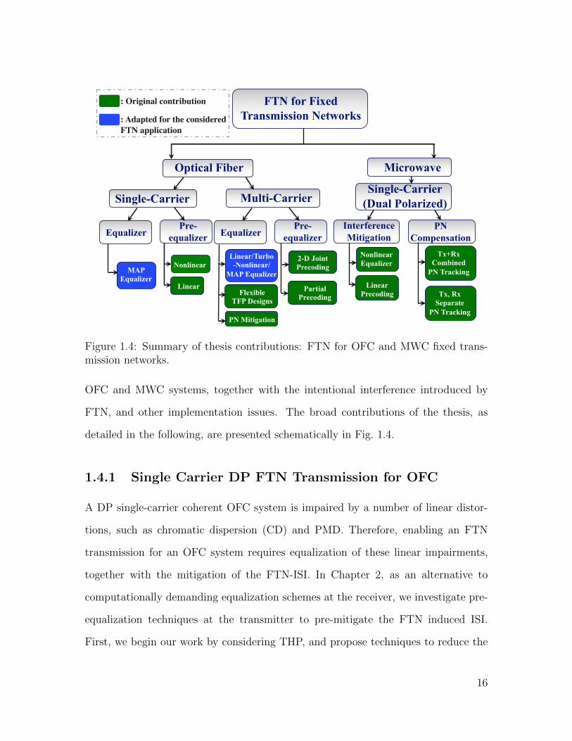
Figure 1.4: Summary of thesis contributions: FTN for OFC and MWC fixed trans-mission networks.

OFC and MWC systems, together with the intentional interference introduced by

FTN, and other implementation issues. The broad contributions of the thesis, as

detailed in the following, are presented schematically in Fig. 1.4.

1.4.1 Single Carrier DP FTN Transmission for OFC

A DP single-carrier coherent OFC system is impaired by a number of linear distor-

tions, such as chromatic dispersion (CD) and PMD. Therefore, enabling an FTN

transmission for an OFC system requires equalization of these linear impairments,

together with the mitigation of the FTN-ISI. In Chapter 2, as an alternative to

computationally demanding equalization schemes at the receiver, we investigate pre-

equalization techniques at the transmitter to pre-mitigate the FTN induced ISI.

First, we begin our work by considering THP, and propose techniques to reduce the

16

modulo-loss. Next, we explore an optimal linear pre-equalization method to com-

pletely eliminate the FTN-ISI. The goal of Chapter 2 is to show that the considered

FTN pre-equalization techniques, as an alternative to computationally prohibitive

receiver-side equalization schemes, have the potential to achieve high SE promised

by FTN signaling. Our contributions in Chapter 2 were published in [87, 88].

1.4.2 Single Carrier DP FTN HoM Transmission for MWC

In order to increase the throughput of the existing SP microwave links, in Chapter 3,

we investigate for the first time a DP-FTN HoM MWC transmission, which suffers

from ISI, XPI, and PN. Being a phase-only impairment in OFC systems, the po-

larization cross-talk can be perfectly equalized by linear filters in such systems [60].

However, in MWC systems, XPI manifests itself as a cross-polarization ISI channel,

and hence, linear equalization may be restrictive in achieving the desired performance.

Moreover, the presence of HoM formats and FTN-ISI further complicates the system

design. The direct application of the already existing algorithms for XPIC and PN

mitigation to the considered DP-FTN HoM system is not straight-forward, because

the channel estimation, FTN and multi-path ISI equalization, and the PN compensa-

tion tasks are not modular, which invites a joint mitigation approach [62, 67]. There-

fore, we investigate joint XPIC and PN compensation techniques for such systems,

since combining the individual solutions is challenging under these circumstances.

2-D DFE and linear pre-equalization methods coupled with CPR are investigated for

this purpose. The general objective of Chapter 3 is to devise powerful interference

cancellation methods for the existing fixed wireless transmission network, such that

a DP-FTN transmission can provide substantial performance improvement over an

equivalent DP-Nyquist system that employs a higher modulation order to achieve the

17

same data rate. The work in Chapter 3 was published in [89, 90].

1.4.3 TFP WDM Superchannel Transmission for OFC

Optical MFTN systems implemented through time-frequency packed superchannels

offer additional SE advantages over single-carrier FTN transmission, at the expense

of introducing controlled ISI and ICI. As an alternative to equalization at the re-

ceiver, in Chapter 4, we investigate an alternative approach of pre-equalizing the

interference at the transmitter, for the first time in an MFTN system where symbols

are packed in both time and frequency dimensions. Despite offering promising per-

formance, the functionality of the precoding techniques in Chapter 4 are limited to

a restricted range of time and frequency compression, which renders the precoding

solutions impractical for high data rate systems. In line with the realistic targets of

Tbps data rates for the futuristic optical WDM systems, we facilitate Terabit TFP

superchannels in Chapter 5, where we investigate low-complexity linear and high-

performance turbo interference mitigation structures, in the presence of additional

aggressive optical filtering. For this, the ISIC and ICIC algorithms in Chapter 5

exploit the known TFP interference channel, without employing additional channel

estimation strategies. However, an interference channel estimation approach can offer

significant performance improvement under these circumstances. Such a flexible and

spectrally efficient TFP transmission targeting Tbps data rates is presented in Chap-

ter 6, together with sophisticated CPR algorithms. This new TFP receiver design

enables us to achieve substantial performance and distance improvements compared

to other competitive TFP solutions. Our contributions in Chapter 4-6 have been

published in [91–93].

18

1.5 Organization of the Thesis

The organization of the thesis, outlined as follows, encompasses the contributions

listed in the previous section.

In Chapter 2, precoded single carrier DP FTN OFC systems are considered. Two

soft demapping algorithms for the nonlinear THP scheme are presented, to reduce

the impact of modulo loss. A new linear pre-equalization method is proposed that

yields optimal performance. We provide numerical results for the coded DP FTN

OFC system to validate the efficiency of the proposed algorithms.

In Chapter 3, we consider for the first time a DP FTN MWC system employing

HoM formats. We propose an XPIC and PN mitigation structure, coupled with

adaptive DFE or linear precoding, to jointly mitigate interference and accomplish

carrier-phase tracking. We present two PN mitigation strategies based on combined

or separate tracking of the transmitter and receiver PN processes. The effectiveness

of the proposed algorithms is demonstrated through computer simulations of a coded

DP-FTN microwave communication system in the presence of PN.

In Chapter 4, we consider precoding for the first time in an MFTN WDM su-

perchannel transmission that enables packing of symbols in both time and frequency

dimensions. For this, we propose two precoding solutions, namely a linear 2-D joint

precoding to pre-equalize TFP-ISI and ICI, and a one-dimensional (1-D) linear pre-

coding followed by turbo equalization at the receiver. Simulation results for precoded

TFP systems are presented the show the benefits of the proposed methods.

In Chapter 5, we compare low-complexity linear and high-performance turbo ICIC

methods to facilitate Tbps optical TFP WDM superchannels. For more complex

structures, BCJR-ISIC in tandem with PIC-ICIC is employed. Aggressive optical fil-

tering is considered in the form of cascades of reconfigurable optical add/drop multi-

19

plexers (ROADMs) implemented via wavelength selective switches (WSSs). Proposed

methods are validated through numerical results.

In Chapter 6, we present flexible designs for Tbps superchannels, where TFP ISI

and ICI channels, PMD equalizer coefficients and a coarse PN are jointly estimated.

Different scheduling algorithms for turbo-ICIC in conjunction with BCJR-ISIC are

investigated. Moreover, we propose powerful iterative methods to mitigate PN stem-

ming from the laser LLW. Simulation results are presented to confirm the advantages

of the proposed schemes.

Finally, in Chapter 7, we provide concluding remarks and future research direc-

tions.

20

Chapter 2

Faster-than-Nyquist Transmission

for Single-Carrier Optical Fiber

Communication Systems

2.1 Introduction

As an enabling technology, FTN is advantageous for transmission systems such as

coherent optical communication where the application of HoM formats to increase

SE renders the system more vulnerable to the nonlinear effects of an optical channel

[11, 33]. To reap the benefits of an FTN transmission, powerful turbo equalization

techniques are employed at the receiver to mitigate the FTN induced ISI [35–41].

However, the complexity of such turbo-equalization methods is substantial. On the

other hand, the low-complexity linear equalization methods are restrictive in achiev-

ing the desired performance.

We, therefore, turn our attention to pre-equalization techniques which can signifi-

cantly diminish or completely eliminate the computational burden from equalization

at the receiver. To this end, the first key observation is that the FTN introduced

ISI is perfectly known at the transmitter. We exploit that knowledge by considering

nonlinear precoding method THP [42–44] and a linear pre-equalization method, to

21

pre-mitigate the effects of FTN-ISI at the transmitter.

In this chapter, as our first contribution, we propose two computationally efficient

demapping algorithms for an FTN-THP system which outperform the existing mem-

oryless demappers from [52, 53] by significant margins. We show that the demappers

presented in this work not only compensate for the modulo-loss but also make THP

competitive to computationally expensive MAP-based equalization techniques. Hav-

ing dealt with the modulo-loss, we then investigate the precoding-loss associated with

THP. For this, we make the second key observation that FTN-ISI stems entirely from

the transmit pulse-shape and the receive matched filter. The transmit pulse-shape

thus contributes partially to the ISI and is a part of the transmitter, whereas, a con-

ventional ISI channel in a Nyquist transmission lies outside the transmitter. As a

consequence, the precoding-loss for an FTN-THP transmission over an AWGN chan-

nel is different from that in a Nyquist-THP transmission over ISI channels. As our

second contribution, we derive the analytical expressions for the precoding-loss in

an FTN-THP system as a function of the FTN and the pulse-shaping parameters.

We show that the precoding-loss of the FTN-THP scheme can be substantial espe-

cially when the ISI induced by FTN becomes severe. Motivated by this, we then

turn our focus on the linear precoding options. In particular, we propose a linear

pre-equalization (LPE) method to pre-compensate for the FTN-ISI. Due to the fact

that FTN is different from classical ISI where the channel lies outside the transmit-

ter, linear pre-equalization does not suffer from noise enhancement. It does, however,

modify the transmit power spectral density (PSD), and we show that our method

converts FTN transmission into orthogonal signaling with an equivalent pulse shape.

In doing so, the proposed LPE completely eliminates FTN-ISI.

The remainder of this chapter is organized as follows. The system model is intro-

22

LDPC

Enc

oder

Inte

rleav

er

QA

M

Map

per RRC

2𝜏𝑇

Opt

ical

Fro

nt-e

nd

DA

C

SSMF

Coh

eren

t Rx.

2x2

MIM

O B

utte

rfly

PM

D E

q.

Dem

appe

r

𝑣′ LDPC

Dec

oder

𝑎

Car

rier R

ecov

ery

FTN

Pr

e-eq

ualiz

er

𝑟

QAMMapper

FTNPre-equalizer

DACRRC Pulse shape

ℎ(𝑡)

QA

M

Map

per

FTN

Pr

e-eq

ualiz

er

DA

C AD

CA

DC

WM

F+

CD

Com

p.

Dem

appe

r De-

inte

rleav

er

𝑣′

𝑎 𝑟

DataIn

DataOutTransmitter Receiver

WF𝐹(𝑧)

WM

F+

CD

Com

p.

SoftDemapper

Rx Matched Filterℎ∗(−𝑡)

AWGN𝜏𝑇-Sampling

Transmitter

Receiver

𝑎 𝑠𝑟

𝑣′

RRC2𝜏𝑇

Interleaver

De-interleaver

FECEncoder

FECDecoder

Data In

Data Out

Figure 2.1: Baseband system model for a pre-equalized FTN transmission wherethe shaded blocks at the transmitter and the receiver represent the proposed FTNpre-equalizer and symbol demappers respectively.

duced in Section 2.2. In Section 2.3, we propose two novel demappers for FTN-THP

and present the analysis for the precoding loss. The new linear pre-filtering method

for FTN is proposed in Section 2.4. In Section 2.5, we validate the proposed methods

based on simulations for a coherent optical transmission setup. Finally, Section 2.6

provides concluding remarks.

2.2 System Model

2.2.1 Precoded FTN

We consider the baseband system model for precoded FTN transmission scheme under

an AWGN channel shown in Fig. 2.1. The system model is common for both linear

and non-linear pre-equalization methods. As shown in Fig. 2.1, the data bits are first

FEC encoded and then the interleaved and modulated data stream a is precoded

with a discrete-time pre-filter to produce the data symbols r. The precoded symbols

r are pulse-shaped by a T -orthogonal pulse h and then transmitted with an FTN

acceleration factor τ < 1. As in [13], the resulting linearly modulated baseband

23

transmitted signal can be written as

s(t) =∑k

r[k]h(t− kτT ) . (2.1)

For the following, we assume a root-raised-cosine (RRC) pulse-shaping filter h with

a roll-off factor β such that∫∞−∞ |h(t)|2dt = 1.

At the receiver, the analog received signal, after passing through the matched-

filter, is sampled at τT -intervals and then digitally processed by a noise whitening

filter (WF) to whiten the colored noise due to FTN. Thereafter, the τT sampled

signal v′ is sent to a symbol demapper to produce soft information in the form of

LLRs for the FEC decoder.

The overall discrete-time channel impulse response between the precoded symbols

r and the output of the τT -spaced sampling is given by

g[n] = (h ∗ f)(nτT ) , (2.2)

where f(t) = h∗(−t), ·∗ is complex conjugate, and ∗ denotes the linear convolu-

tion. We also introduce G = Z(g), where Z{·} denotes the z-transform. In a

Nyquist-system (τ = 1), T -orthogonality of the pulse-shape h along with the condi-

tion∫∞−∞ |h(t)|2dt = 1 makes G(z) = 1. But for an FTN transmission with τ < 1,

G(z) causes ISI across consecutive transmitted symbols.

As THP can be seen as a dual to a DFE performed at the receiver [44], we apply

a spectral factorization to G (consistent with [44, 94]) as detailed in the following

subsection.

24

2.2.2 Spectral Factorization

THP requires the implementation of a feed-forward-filter (FFF) F and a feedback-

filter (FBF) B to pre-equalize the ISI due to FTN. As the noise samples after the

τT -sampler in an FTN system are colored, the purpose of the FFF is then two-fold:

to whiten the received noise samples and to shape the end-to-end channel transfer-

function into a causal and minimum-phase response [44]. The FBF is then used

as a pre-filter at the transmitter to pre-equalize the overall effective ISI-channel.

Computation of FFF and FBF requires the discrete-time spectral factorization [44]

G(z) = αQ(z)Q∗(z−∗), (2.3)

such that Q(z) is casual, monic and minimum-phase and α > 0 is a scaling factor used

to make Q(z) monic. The necessary and sufficient condition for the realization of the

above spectral factorization (see e.g. [44, 95]) can be written in an FTN transmission

as

τT

∫ 12τT

− 12τT

| log(G(ej2πfτT )

)|df <∞ . (2.4)

Since from (2.2),

G(ej2πfτT ) =1

τT

∞∑k=−∞

|H(f − k/(τT ))|2 , (2.5)

where H is the Fourier-transform of the pulse-shaping filter h. We note thatG(ej2πfτT )

in (2.5) is zero in the intervals[− 1

2τT,−1+β

2T

]and

[1+β2T, 1

2τT

]when the FTN acceler-

ation factor τ < 11+β

. This causes the condition in (2.4) to fail, which consequently

makes the spectral factorization (2.3) required for THP unrealizable. Hence, in the

following we restrict ourselves to FTN with τ ≥ 11+β

for a given β. Once the fac-

torization according to (2.3) is executed, we obtain the FFF and FBF respectively

25

Modulo2M

+

-

V1(z)-1

a[k] x[k]

THP

f[k]

= = +

-

V1(z)-1

v[k] x[k]

f[k]

a[k]

d[k]

FTNPre-equalizer

≡ +

-Modulo2M

FBFB(z)-1

≡𝑎

𝑓

𝑟 +

-

FBFB(z)-1

𝑎 𝑟𝑑

𝑣

≡ +

-

FBFB(z)-1

𝑎

𝑓

𝑟FTNPre-equalizer

≡ +

-Modulo2M

FBFB(z)-1

𝑎

𝑓

𝑟

++

Figure 2.2: FTN pre-equalization with THP and the modulo-equivalent linear struc-ture.

as

F (z) =1

αQ∗ (z−∗)and B(z) = Q(z) . (2.6)

Using the FFF and FBF computed above, we now proceed to introduce FTN-THP

with an improved demapper in the next section, and a new linear pre-equalization

method in Section 2.4.

2.3 Non-linear Precoding in FTN Systems

In this section, we consider non-linear precoding for FTN in the form of THP.

2.3.1 THP-precoded FTN

Since the effective ISI-channel caused by FTN is a-priori known at the transmitter,

the filters from Section 2.2.2 can be computed and applied for THP without any

feedback from the receiver.

Fig. 2.2 depicts the detailed diagram and the associated linear equivalent structure

of the block “FTN Pre-equalizer” from Fig. 2.1. The modulo operation in a classical

THP system as shown in Fig. 2.2 is used to keep the output stable especially for

26

channels with spectral zeros by bounding it within a well-prescribed range [44]. The

input symbols a in Fig. 2.2 consist of the modulated symbols and the feedback filter B,

as given in (2.6), is a function of the FTN parameter τ and the pulse shape h. As the

FTN-ISI is real-valued, without loss of generality, we assume that the symbols a are

drawn from an M -ary 1-D constellation. In the equivalent linear representation, the

modulo operation of THP is replaced by an equivalent addition of a unique sequence

d to the data symbols a so that precoded symbols r lie in the interval [−M,M).

The combination of a and d produces the intermediate signal v, the elements of

which are taken from an extended constellation with more than M signal points. In

an ideal noise-free scenario, the signal v′ in Fig. 2.1 is same as v of Fig. 2.2, and

thus, to compensate for THP, conventionally a modulo operation is performed on

v′ at the receiver. However, for noisy channels and particularly for a relatively low

SNR, this modulo operation is sub-optimal which makes the LLR computation by a

conventional soft-demapper unreliable. These inaccurate LLRs are then passed on to

the FEC decoder as shown in Fig. 2.1 and thereby causing a performance degradation,

especially in an FEC coded transmission, which is commonly known as the “modulo

loss”.

To overcome this loss, a modified modulo based demapper for a coded THP system

was proposed in [52] and its simplified implementation method was also presented

recently in [53]. However, the residual modulo-loss of these approaches still causes a

significant loss in the bit-error rate (BER). Another near-optimal iterative method

was shown in [54]. It is based on a quantized-output THP, and its computational

complexity is of the order of MAP equalization. In the following, we present two rela-

tively simpler soft-demapping algorithms which significantly outperform the demap-

per from [52], which we refer to as Peh-Liang-Demapper (PLD), and are competitive

27

to optimal MAP equalization in terms of BER.

2.3.2 Expanded A-priori Demapper (EAD)

In order to counter the modulo-loss, we replace the modulo operation of a conventional

THP demapper with our proposed new demapper, referred to as EAD, which now

forms the module “Soft Demapper” of Fig. 2.1. The proposed EAD is based on the lin-

ear equivalent model from Fig. 2.2 and considers the extended constellation of the in-

termediate data signal v to compute LLRs. LetA = {aκPAM = ±1,±3, . . . ,±(M − 1)}

be the set of M -ary pulse-amplitude modulation (PAM) constellation symbols. Then,

the symbols v belong to the extended signal set V = {v[k]} = A + 2MZ. In par-

ticular, we note that the probabilities of the signal points v ∈ V are not uniform.

Therefore, the EAD computes the LLR value corresponding to the nth bit bn of the

kth data symbol a[k] as

LLREADk,n = log

(Pr (bn = 1|v′[k])

Pr (bn = 0|v′[k])

)(2.7)

= log

∑c∈C1,n

Pr(v′[k]|v[k]=c) Pr(v[k]=c)∑c∈C0,n

Pr(v′[k]|v[k]=c) Pr(v[k]=c), (2.8)

where Ci,n is the subset of symbols in V corresponding to the nth bit being equal to

i ∈ {0, 1} and v′[k] is the kth received sample at the demapper input. The relation

between v and v′ follows as

v′[k] = v[k] + η[k] , (2.9)

28

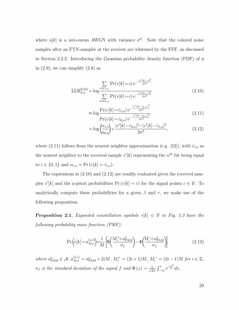
where η[k] is a zero-mean AWGN with variance σ2. Note that the colored noise

samples after an FTN-sampler at the receiver are whitened by the FFF, as discussed

in Section 2.2.2. Introducing the Gaussian probability density function (PDF) of η

in (2.9), we can simplify (2.8) as

LLREADk,n = log

∑c∈C1,n

Pr(v[k]=c) e−|v′[k]−c|2

2σ2

∑c∈C0,n

Pr(v[k]=c) e−|v′[k]−c|2

2σ2

(2.10)

≈ logPr(v[k]= c1,n) e−

|v′[k]−c1,n|2

2σ2

Pr(v[k]= c0,n) e−|v′[k]−c0,n|2

2σ2

(2.11)

= log

(α1,n

α0,n

)+|v′[k]−c0,n|2−|v′[k]−c1,n|2

2σ2, (2.12)

where (2.11) follows from the nearest neighbor approximation (e.g. [52]), with ci,n as

the nearest neighbor to the received sample v′[k] representing the nth bit being equal

to i ∈ {0, 1} and αi,n = Pr (v[k] = ci,n).

The expressions in (2.10) and (2.12) are readily evaluated given the received sam-

ples v′[k] and the a-priori probabilities Pr (v[k] = c) for the signal points c ∈ V . To

analytically compute these probabilities for a given β and τ , we make use of the

following proposition.

Proposition 2.1. Expanded constellation symbols v[k] ∈ V in Fig. 2.2 have the

following probability mass function (PMF):

Pr(v[k]=a

(κ,i)M,v

)=

1

M

[Φ

(M+

i+aκPAM

σf

)−Φ

(M−

i+aκPAM

σf

)], (2.13)

where aκPAM ∈ A, a(κ,i)M,v = aκPAM + 2iM , M+

i = (2i+ 1)M , M−i = (2i− 1)M for i ∈ Z,

σf is the standard deviation of the signal f and Φ (x) = 1√2π

∫ x−∞ e

−x2

2 dx.

29

Proof. See Appendix A.1.

The standard deviation σf in (2.13) can be computed numerically. Simulation

results in Section 2.5 show that EAD can offer substantial gains over PLD especially

when the FTN-ISI is less severe. The relation between the LLR calculation by EAD

and PLD from [52] for severe FTN-ISI is summarized in the following proposition

and its corollary.

Proposition 2.2. For 2PAM and 4PAM modulations, the LLR expression in (2.12)

becomes equivalent to the approximate LLR expression computed by PLD as given

in [52] if the extended constellation symbols of the signal v are assumed to have equal

probabilities.


Corollary 2.2.1. For 2PAM and 4PAM modulations, when the FTN-ISI becomes

severe (i.e. τ reduces for a given RRC roll-off β), the LLR expressions computed by

EAD and PLD become similar.

Proof. For an M -ary PAM constellation, an upper bound on the maximum number

of signal points in V with non-zero probability is given in [44] as

Vmax = 2

⌊M∑P−1

k=0 |b[k]|+ 1

2

⌋− 1 , (2.14)

where b = Z−1(B) is the THP feedback filter response, P denotes the length of the ISI

channel and the function bxc denotes the largest integer contained in x. Therefore,

with large P , V contains more symbols with non-zero probabilities which causes the

bell-shaped PMF in (2.13) to flatten and its shape starts resembling closer to that of

a uniform distribution. Then by Proposition 2.2, LLRs computed by EAD become

similar to those computed by PLD.

30

As evaluated above, the gains offered by EAD reduce for decreasing τ . This can

be attributed to the fact that while EAD takes the probabilities of the extended

constellation symbols into account, it fails to incorporate the auto-correlation of

the intermediate symbol sequence v into the LLR metric in (2.12). As τ reduces,

correlation between successive symbols of v can increase significantly due to severe

FTN-ISI. In order to account for this, we present the second demapper design in the

following.

2.3.3 Sliding-Window-EAD (SW-EAD)

The SW-EAD includes L preceding and succeeding observations (corresponding to

a sliding window of length 2L + 1) into the computation of LLRs for the current

symbol. Depending on the severity of the ISI and the observed auto-correlation of

v, a suitable value L is determined. The modified LLR for the nth bit bn of the kth

transmitted symbol a[k] is computed as

LLRSW-EADk,n =log

(Pr(bn=1|v′[k−L],. . . ,v′[k+L])

Pr(bn=0|v′[k−L],. . . ,v′[k+L])

)(2.15)

= log

∑

c∈C1,n,v[k−L],...,v[k+L]

Pr(

#»

v′ | #»v c)

Pr ( #»v c)∑c∈C0,n,v[k−L],...,v[k+L]

Pr(

#»

v′ | #»v c)

Pr ( #»v c)

(2.16)

= log

∑

c∈C1,n,v[k−L],...,v[k+L]

Pr ( #»v c) e−‖

#»

v′− #»v c‖2

2σ2

∑c∈C0,n,v[k−L],...,v[k+L]

Pr ( #»v c) e−‖

#»

v′− #»v c‖22σ2

, (2.17)

31

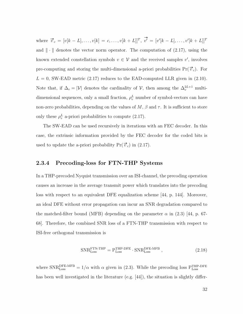
where #»v c = [v[k − L], . . . , v[k] = c, . . . , v[k + L]]T ,#»

v′ = [v′[k − L], . . . , v′[k + L]]T

and ‖ · ‖ denotes the vector norm operator. The computation of (2.17), using the

known extended constellation symbols v ∈ V and the received samples v′, involves

pre-computing and storing the multi-dimensional a-priori probabilities Pr( #»v c). For

L = 0, SW-EAD metric (2.17) reduces to the EAD-computed LLR given in (2.10).

Note that, if ∆v = |V| denotes the cardinality of V , then among the ∆2L+1v multi-

dimensional sequences, only a small fraction, ρLv number of symbol-vectors can have

non-zero probabilities, depending on the values of M , β and τ . It is sufficient to store

only these ρLv a-priori probabilities to compute (2.17).

The SW-EAD can be used recursively in iterations with an FEC decoder. In this

case, the extrinsic information provided by the FEC decoder for the coded bits is

used to update the a-priori probability Pr( #»v c) in (2.17).

2.3.4 Precoding-loss for FTN-THP Systems

In a THP-precoded Nyquist transmission over an ISI-channel, the precoding operation

causes an increase in the average transmit power which translates into the precoding

loss with respect to an equivalent DFE equalization scheme [44, p. 144]. Moreover,

an ideal DFE without error propagation can incur an SNR degradation compared to

the matched-filter bound (MFB) depending on the parameter α in (2.3) [44, p. 67-

68]. Therefore, the combined SNR loss of a FTN-THP transmission with respect to

ISI-free orthogonal transmission is

SNRFTN-THPLoss = PTHP-DFE

Loss · SNRDFE-MFBLoss , (2.18)

where SNRDFE-MFBLoss = 1/α with α given in (2.3). While the precoding loss PTHP-DFE

Loss

has been well investigated in the literature (e.g. [44]), the situation is slightly differ-

32

ent for FTN-THP systems, where the transmit power and hence the precoding loss

depend on the ISI channel through the transmit pulse-shape. In order to quantify

the precoding loss, we utilize the results from the following proposition.

Proposition 2.3. For an FTN-THP system with the FFF and FBF given in (2.6),

the PSD of the transmitted signal is given by

ΦTHPss (f) = αΦvv

(ej2πτfT

) G(f)∑k

G(f + k

τT

) , (2.19)

and the average transmitted power is

PTHPAvg =

ασ2v

τT, (2.20)

where σ2v and Φvv

(ej2πτfT

)are the variance and the PSD of the extended constellation

symbols v, respectively, G(f) = |H(f)|2, and α > 0 is the constant given in (2.3).


Since (i) a THP and a DFE system with the same FFF and FBF perform iden-

tically assuming no modulo loss for THP and no error propagation for DFE and (ii)

the transmit power for non-precoded FTN is PAvg = σ2a

τT, where σ2

a is the variance of

the M -ary constellation symbol a (e.g. [13]), we have from (2.20) that

PTHP-DFELoss = α

σ2v

σ2a

. (2.21)

The overall SNR-loss of the FTN-THP system as compared to the ISI-free transmis-

33

Modulo2M

+

-

V1(z)-1

a[k] x[k]

THP

f[k]

= = +

-

V1(z)-1

v[k] x[k]

f[k]

a[k]

d[k]

FTNPre-equalizer

≡ +

-Modulo2M

FBFB(z)-1

≡𝑎

𝑓

𝑟 +

-

FBFB(z)-1

𝑎 𝑟𝑑

𝑣

≡ +

-

FBFB(z)-1

𝑎

𝑓

𝑟FTNPre-equalizer

≡ +

-Modulo2M

FBFB(z)-1

𝑎

𝑓

𝑟

++

Figure 2.3: Linear pre-equalization of FTN ISI.

sion follows from (2.18) as

SNRFTN-THPLoss =

σ2v

σ2a

. (2.22)

2.4 Linear Pre-equalization for FTN

FTN-THP not only incurs an SNR loss, but it may also complicate pilot-based chan-

nel estimation. Since the THP operation results in an expanded signal constellation

v′ after the WF stage shown in Fig. 2.1, the receiver lacks the prior knowledge of the

exact representation of pilot symbols introduced into the data stream. To alleviate

this problem, careful attention to the pilot-symbol design is needed [48] or a coarse

detection of the pilot symbol is required before channel estimation [49].

These problems warrant the consideration of linear precoding or pre-equalization

methods. We note that linear precoding is done in PRS transmission, albeit the pur-

pose is not pre-equalization but spectral shaping of the transmit signal or the maxi-

mization of some performance criteria assuming receiver-side equalization [13, 55–57].

Different from this, we propose a linear pre-equalization (LPE) technique to mitigate

the ISI introduced through FTN signaling. More specifically, the pre-equalization

is achieved through a linear pre-filtering method which is derived from the THP

34

transmitter structure by dropping the modulo operator as shown in Fig. 2.3. The

exclusion of the modulo function renders the overall transmitter of Fig. 2.3 a linear

infinite impulse response (IIR) filtering operation. The minimum-phase property of

the feedback filter B(z), as discussed in Section 2.2.2, guarantees the stability of the

IIR filter.

In Nyquist transmission over ISI channels, linear pre-equalization is usually not

a preferred choice. In particular, linear pre-equalization to eliminate ISI results in

an elevation of the average transmitted power, which creates a similar error-rate

degradation as the noise-enhancement phenomena encountered in a linear zero-forcing

equalization [44]. However, as pointed out earlier, in an FTN transmission, the ISI

stems from the transmitter pulse-shape and receiver matched filter. In particular,

the feedback filter B in Fig. 2.3 is a function of the RRC filter h related through

(2.3), (2.5) and (2.6). This leads to the following results for the PSD and the average

transmit power for FTN-LPE transmission.

Proposition 2.4. For an FTN-LPE system in Fig. 2.3 with the FBF given in (2.6),

the PSD of the transmitted signal is given by

ΦLPEss (f) = ασ2

a

G(f)∑k

G(f + k

τT

) , (2.23)

and the average transmit power is

P LPEAvg =

ασ2a

τT, (2.24)

where σ2a is the variance of the input constellation symbols a and α > 0 is given in

(2.3).


35

Corollary 2.4.1. For a Nyquist system, the transmitted PSD becomes ΦNyqss (f) =

σ2a

TG(f) with an average transmitted power PNyq

Avg = σ2a

T.

Proof. For a Nyquist system, τ = 1, α = 1 from (2.3) and 1T

∑k

G(f + k

T

)= 1.

Putting these values in (2.23) and (2.24) yields the well-known expressions.

Corollary 2.4.2. If τ = 11+β

, the PSD of the transmitted signal becomes rectangular

with a bandwidth 1+βT

.

Proof. The expression∑k

G(f + k

τT

)in (2.23) is the sum of the frequency-shifted

replicas of G(f), where the frequency shifts are integral multiples of 1τT

. We note

that,

G(f) = 0 ,when |f | > 1 + β

2T. (2.25)

Therefore, when τ = 11+β

, there are no overlaps between the replicas of G in∑k

G(f + k

τT

).

Consequently,∑k

G(f + k

τT

)= G(f) in the frequency range −1+β

2T≤ f ≤ 1+β

2T. Thus,

from (2.23) we have

ΦLPEss (f) =

ασ2a, −

1+β2T≤ f ≤ 1+β

2T

0, otherwise(2.26)

To investigate the power-penalty of the FTN-LPE transmission, we use the same

procedure which was adopted in Section 2.3.4 for the SNR-loss computation of an

FTN-THP system. Similar to (2.18), we can write the combined SNR-loss for the

LPE as

SNRFTN-LPELoss = PLPE-DFE

Loss · SNRDFE-MFBLoss , (2.27)

36

where SNRDFE-MFBLoss = 1/α as in (2.18) and following the same reasoning as in Section

2.3.4, the precoding loss PLPE-DFELoss can be computed from (2.24) as

P LPE-DFELoss = α . (2.28)

Hence, the overall SNR-loss of the LPE-THP system as compared to the ISI-free

transmission can be written from (2.27) as

SNRFTN-LPELoss = 1 . (2.29)

We conclude from (2.29) that FTN-LPE does not suffer from a power penalty due

to channel inversion and achieves the same error-rate performance as an ISI-free

transmission. To do so, linear pre-equalization modifies the transmit PSD according

to (2.23) that exhibits τT -orthogonality. In fact, a closer inspection of the FBF

and FFF filters for LPE reveals that the combination of the LPE pre-filter and the

RRC pulse-shape at the transmitter is equivalent to a new τT -orthogonal square-root

Nyquist pulse-shaping filter 3. Similarly, at the receiver, the RRC filter, combined

with the WF, constitutes an equivalent square-root Nyquist matched-filter to the

new transmit pulse-shape. Hence, FTN-LPE with whitened matched-filtering and

τT sampling is ISI-free.

As an alternative τT -orthogonal signaling scheme, one could directly use a τT -

orthogonal RRC filter with roll-off β = τ(1 + β)− 1 for transmit pulse-shaping. For

instance, an FTN system with T -orthogonal RRC having β = 0.3 and τ = 0.78 results

in an effective β = 0.014 for the direct τT -orthogonal RRC design. We illustrate in

Section 2.5 that due to the stricter roll-off requirement for this new RRC pulse-shape,

3Because of this, we remark that our LPE design with FTN signaling can be viewed as a practicalapproach for Brickwall filter implementation.

37

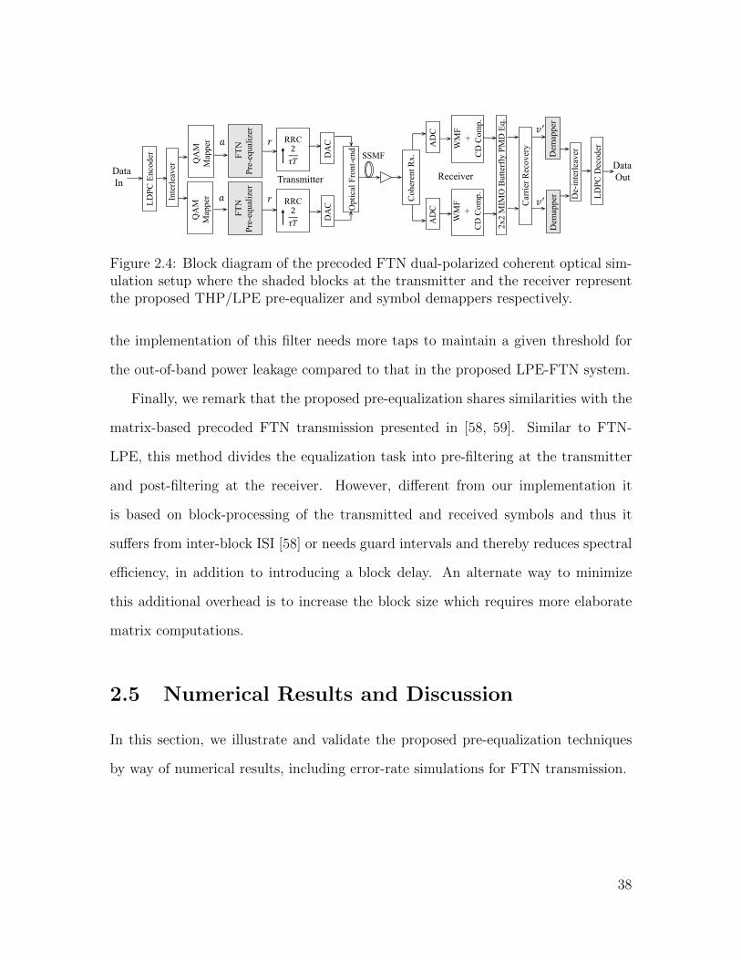
LDPC

Enc

oder

Inte

rleav

er

QA

M

Map

per RRC

2𝜏𝑇

Opt

ical

Fro

nt-e

nd

DA

C

SSMF

Coh

eren

t Rx.

2x2

MIM

O B

utte

rfly

PM

D E

q.

Dem

appe

r

𝑣′ LDPC

Dec

oder

𝑎

Car

rier R

ecov

ery

FTN

Pr

e-eq

ualiz

er

𝑟

QAMMapper

FTNPre-equalizer

DACRRC Pulse shape

ℎ(𝑡)

QA

M

Map

per

FTN

Pr

e-eq

ualiz

er

DA

C AD

CA

DC

WM

F+

CD

Com

p.

Dem

appe

r De-

inte

rleav

er

𝑣′

𝑎 𝑟

DataIn

DataOutTransmitter Receiver

WF𝐹(𝑧)

WM

F+

CD

Com

p.

SoftDemapper

Rx Matched Filterℎ∗(−𝑡)

AWGN𝜏𝑇-Sampling

Transmitter

Receiver

𝑎 𝑠𝑟

𝑣′

RRC2𝜏𝑇

Interleaver

De-interleaver

FECEncoder

FECDecoder

Data In

Data Out

Figure 2.4: Block diagram of the precoded FTN dual-polarized coherent optical sim-ulation setup where the shaded blocks at the transmitter and the receiver representthe proposed THP/LPE pre-equalizer and symbol demappers respectively.

the implementation of this filter needs more taps to maintain a given threshold for

the out-of-band power leakage compared to that in the proposed LPE-FTN system.

Finally, we remark that the proposed pre-equalization shares similarities with the

matrix-based precoded FTN transmission presented in [58, 59]. Similar to FTN-

LPE, this method divides the equalization task into pre-filtering at the transmitter

and post-filtering at the receiver. However, different from our implementation it

is based on block-processing of the transmitted and received symbols and thus it

suffers from inter-block ISI [58] or needs guard intervals and thereby reduces spectral

efficiency, in addition to introducing a block delay. An alternate way to minimize

this additional overhead is to increase the block size which requires more elaborate

matrix computations.

2.5 Numerical Results and Discussion

In this section, we illustrate and validate the proposed pre-equalization techniques

by way of numerical results, including error-rate simulations for FTN transmission.

38

2.5.1 Simulation Setup

For the simulations, we consider a coherent optical single-carrier (COSC) transmission

system. Optical communication systems are a prime candidate for the introduction

of FTN as the use of higher-order modulation is challenging in such systems [11,

33]. The block diagram of a COSC system with polarization division multiplexing

is shown in Fig. 2.4. The precoding algorithms presented hitherto, considering the

AWGN system model in Fig. 2.1, are directly applicable to linear optical channels

as impairments such as CD and PMD can be compensated through a proper two-

dimensional equalizer [60].

In Fig. 2.4, the transmitter and receiver blocks for the discrete-time baseband

modules are same as those in Fig. 2.1 except that the data processing for each of

the two polarizations is performed separately. For our simulations, we use a low-

density parity-check (LDPC) code of rate 0.8, a random bit-interleaver, QPSK and

16-ary quadrature amplitude modulation (16QAM) formats, and a fixed baud rate

of 32 Gbaud for all values of τ . The RRC pulse-shaping filter is implemented with

2-times oversampling having 73 time-domain taps with β = 0.3, and the THP/LPE

precoders are designed using 10-taps for the feedback filter. The baseband analog

data after the digital-to-analog converter (DAC) is processed by the opto-electronic

front-end and transmitted as an optical signal through a 1000 km standard single-

mode fiber (SSMF) with CD and mean PMD parameter values of −22.63 ps2/km

and 0.8 ps/√

km, respectively, and then is received by the optical coherent receiver.

The whitened matched filter (WMF) is combined with the time-invariant frequency

domain CD compensator using overlap-and-add method. For PMD compensation, we

used a 13-tap 2×2 butterfly-type fractionally-spaced adaptive LMS equalizer [60, 96].

Following carrier recovery, the QAM-demapper computes and passes on LLR values

39

8 9 10 11 12 13 14 1510

−6

10−5

10−4

10−3

10−2

10−1

OSNR [dB]

BE

R

Nyquist (τ = 1)

τ = 0.85

τ = 0.8

CTHP

0.9 dB

MAP

EADPLD

1.65 dB

4.2 dB

Figure 2.5: BER vs. OSNR for FTN-THP with different demappers, illustrating theperformance of the proposed EAD. QPSK, β = 0.3, τ = 0.85 and 0.8.

to the LDPC decoder.

2.5.2 Performance of FTN-THP with Proposed Demappers

We first compare the performance of FTN-THP using the proposed EAD scheme with

respect to the conventional THP (CTHP) demapper which employs a modulo oper-

ation at the receiver and the modulo-based PLD proposed in [52, 53]. Fig. 2.5 shows

the coded BER performance as a function of the optical SNR (OSNR) for different

FTN parameters τ with QPSK modulation. We also include the BER performance

with MAP equalization, which considers 6-taps of the ISI channel and performs 10

40

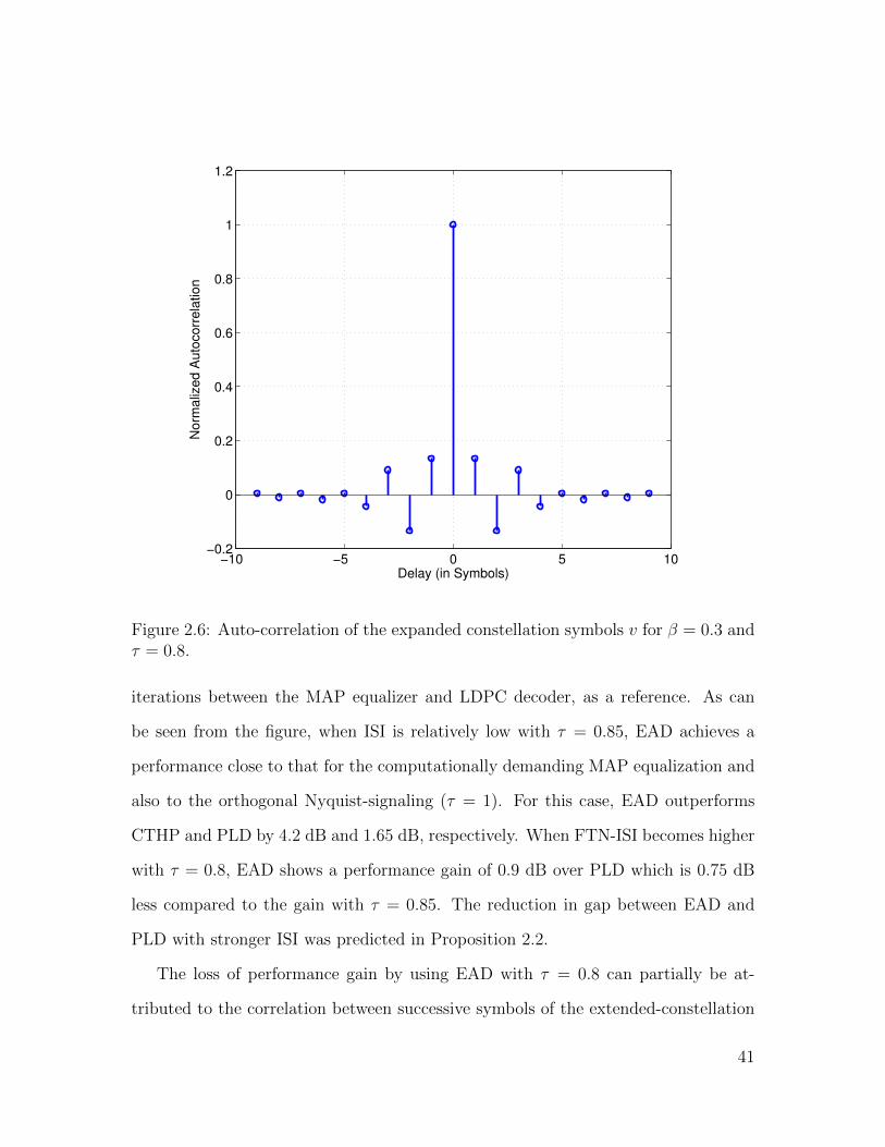
−10 −5 0 5 10−0.2

0

0.2

0.4

0.6

0.8

1

1.2

Delay (in Symbols)

Norm

aliz

ed A

uto

corr

ela

tion

Figure 2.6: Auto-correlation of the expanded constellation symbols v for β = 0.3 andτ = 0.8.

iterations between the MAP equalizer and LDPC decoder, as a reference. As can

be seen from the figure, when ISI is relatively low with τ = 0.85, EAD achieves a

performance close to that for the computationally demanding MAP equalization and

also to the orthogonal Nyquist-signaling (τ = 1). For this case, EAD outperforms

CTHP and PLD by 4.2 dB and 1.65 dB, respectively. When FTN-ISI becomes higher

with τ = 0.8, EAD shows a performance gain of 0.9 dB over PLD which is 0.75 dB

less compared to the gain with τ = 0.85. The reduction in gap between EAD and

PLD with stronger ISI was predicted in Proposition 2.2.

The loss of performance gain by using EAD with τ = 0.8 can partially be at-

tributed to the correlation between successive symbols of the extended-constellation

41

8.5 9 9.5 10 10.5 1110

−6

10−5

10−4

10−3

10−2

10−1

OSNR [dB]

BE

R

EAD (L = 0)

SW−EAD (L = 1)

SW−EAD (L = 1), 10 it.

SW−EAD (L = 3)

SW−EAD (L = 3), 10 it.

MAP

Nyquist (τ = 1)

0.8 dB1.3 dB

Figure 2.7: BER vs. OSNR for FTN-THP with different demappers, illustratingthe performance gains with the proposed SW-EAD over EAD. QPSK, β = 0.3 andτ = 0.8.

sequence v of Fig. 2.2. The auto-correlation sequence of v is plotted in Fig. 2.6. This

correlation is not taken into account while computing the EAD-LLR metric in (2.12).

Fig. 2.7 shows the additional performance gains obtained by SW-EAD over EAD.

The different curves represent distinct values of L corresponding to the SW-EAD

window-length (2L + 1) with and without iterations between the demapper and the

LDPC decoder. We observe that SW-EAD get improvements of the order of 0.8 dB

over EAD which makes it competitive to MAP equalization. With higher values of

L, further improvements for SW-EAD are not expected as only up to 3−4 significant

taps are observed in Fig. 2.6.

42

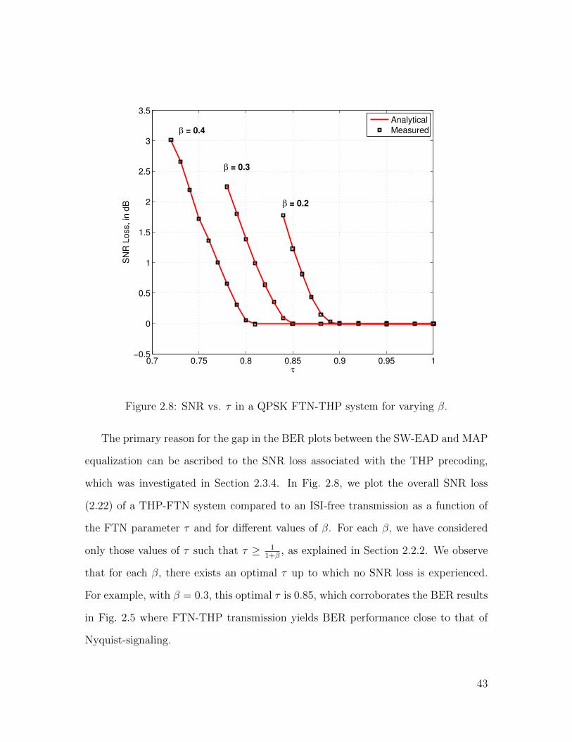
0.7 0.75 0.8 0.85 0.9 0.95 1−0.5

0

0.5

1

1.5

2

2.5

3

3.5

τ

SN

R L

oss,

in d

B

Analytical

Measuredβ = 0.4

β = 0.3

β = 0.2

Figure 2.8: SNR vs. τ in a QPSK FTN-THP system for varying β.

The primary reason for the gap in the BER plots between the SW-EAD and MAP

equalization can be ascribed to the SNR loss associated with the THP precoding,

which was investigated in Section 2.3.4. In Fig. 2.8, we plot the overall SNR loss

(2.22) of a THP-FTN system compared to an ISI-free transmission as a function of

the FTN parameter τ and for different values of β. For each β, we have considered

only those values of τ such that τ ≥ 11+β

, as explained in Section 2.2.2. We observe

that for each β, there exists an optimal τ up to which no SNR loss is experienced.

For example, with β = 0.3, this optimal τ is 0.85, which corroborates the BER results

in Fig. 2.5 where FTN-THP transmission yields BER performance close to that of

Nyquist-signaling.

43

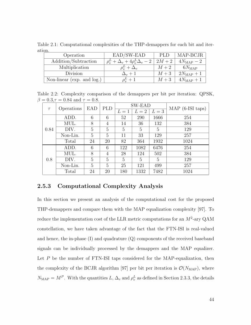
Table 2.1: Computational complexities of the THP-demappers for each bit and iter-ation.

Operation EAD/SW-EAD PLD MAP-BCJRAddition/Subtraction ρLv + ∆v + 4ρLv∆v − 2 2M + 2 4NMAP − 2

Multiplication ρLv + ∆v M + 2 6NMAP

Division ∆v + 1 M + 3 2NMAP + 1Non-linear (exp. and log.) ρLv + 1 M + 3 4NMAP + 1

Table 2.2: Complexity comparison of the demappers per bit per iteration: QPSK,β = 0.3,τ = 0.84 and τ = 0.8.

τ Operations EAD PLDSW-EAD

MAP (6-ISI taps)L = 1 L = 2 L = 3

0.84

ADD. 6 6 52 290 1666 254MUL. 8 4 14 36 132 384DIV. 5 5 5 5 5 129

Non-Lin. 5 5 11 33 129 257Total 24 20 82 364 1932 1024

0.8

ADD. 6 6 122 1082 6476 254MUL. 8 4 28 124 502 384DIV. 5 5 5 5 5 129

Non-Lin. 5 5 25 121 499 257Total 24 20 180 1332 7482 1024

2.5.3 Computational Complexity Analysis

In this section we present an analysis of the computational cost for the proposed

THP-demappers and compare them with the MAP equalization complexity [97]. To

reduce the implementation cost of the LLR metric computations for an M2-ary QAM

constellation, we have taken advantage of the fact that the FTN-ISI is real-valued

and hence, the in-phase (I) and quadrature (Q) components of the received baseband

signals can be individually processed by the demappers and the MAP equalizer.

Let P be the number of FTN-ISI taps considered for the MAP-equalization, then

the complexity of the BCJR algorithm [97] per bit per iteration is O(NMAP), where

NMAP = MP . With the quantities L, ∆v and ρLv as defined in Section 2.3.3, the details

44

of the mathematical operations, required for implementing the EAD and SW-EAD

LLR metrics for each bit in each iteration according to (2.10) and (2.17) respectively,

are furnished in Table 2.1. To illustrate this analysis with further clarity and ease

of comparison, two specific examples are provided in Table 2.2 with τ = 0.84 and

τ = 0.8 for β = 0.3 and QPSK modulation.

The numbers in Table 2.2 reveal that the implementation complexities of the LLR

metrics computed by EAD in (2.10) and PLD are similar for the FTN transmissions

studied in this chapter, even though EAD demonstrated substantial performance

gains over PLD as shown in Section 2.5.2. Moreover, Table 2.2 shows that while

EAD is significantly more computationally efficient than the MAP equalization, the

complexity of the SW-EAD rises with increasing window size, especially for low values

of τ . We recall from Section 2.5.2 that the SW-EAD performance is always limited

even when the window parameter L increases infinitely, as illustrated in Fig. 2.7. This

is because SW-EAD can successfully remove the modulo-loss but fails to improve the

power-penalty (SNR-loss) associated with an FTN-THP transmission. Therefore, for

a given complexity requirement on the receiver side processing, RRC roll-off β and

FTN parameter τ , the window parameter L and the number of iterations between

the SW-EAD and the LDPC decoder should be wisely chosen as a desired trade-off

between performance and complexity.

2.5.4 Performance of Proposed FTN-LPE

As described in Section 2.3.4 and shown in Fig. 2.8, an SNR degradation is inherent to

THP precoding for some values of τ and β. Our proposed LPE scheme can overcome

this problem. Fig. 2.9 shows the FTN-LPE BER results for QPSK and 16QAM.

We observe that LPE precoding produces an optimal performance, i.e., the BER is

45

8 10 12 14 16 18 20 2210

−6

10−5

10−4

10−3

10−2

10−1

OSNR, dB

BE

R

Nyquist

LPE

MAP

EAD

PLD

CTHP

16−QAM

τ = 0.85

QPSK

τ = 0.8

Figure 2.9: BER vs. OSNR for FTN with LPE precoding. QPSK with τ = 0.8 and16QAM with τ = 0.85, β = 0.3.

identical to that of orthogonal signaling. The figure also includes the BER curves

from Fig. 2.5 with τ = 0.8 to show the gains offered by LPE over THP. Similar

observations hold true with higher order modulation, such as 16QAM.

The optimal BER performance of LPE precoded FTN systems comes at the

expense of transmitted spectral shape modification, as investigated in Section 2.4.

Fig. 2.10 plots the normalized analytical transmit PSDs of the LPE precoded FTN

system, which was derived in (2.23). We also include the normalized PSDs for (non-

precoded) Nyquist signaling using the underlying T -orthogonal RRC with β = 0.3

and a τT -orthogonal RRC with β = τ(1 + β)− 1 = 0.105 for pulse shaping, respec-

tively. For this comparison, all three systems use the same bandwidth, which implies

46

0 0.2 0.4 0.60

0.2

0.4

0.6

0.8

1

0.6

0.7

0.8

0.9

1

fT

Norm

aliz

ed P

SD

(T

heore

tical)

T-Orthogonal RCLPE

Alternate RC (β = 0.105)

Figure 2.10: Normalized PSD of LPE-FTN vs. normalized frequency fT for β = 0.3,τ = 0.85. Also included are the PSDs for Nyquist signaling with the T -orthogonalRRC with β = 0.3 and the τT -orthogonal RRC with β = 0.105.

that the LPE-FTN system and the Nyquist-system with the RRC with β = 0.105

operate at a higher baud rate. We observe that with LPE precoding, the overall PSD

behaves as a τT -orthogonal pulse-shape. That is, the PSD has a odd-symmetry about

the normalized frequency fT = 12τ

= 0.59 similar to the alternate τT -orthogonal RC.

The advantage of the proposed LPE scheme over a direct τT -orthogonal RRC

pulse-shaping is illustrated in Fig. 2.11 in terms of the out-of-band emission perfor-

mance. Here, the transmit pulse-shaping filters for both the LPE precoded FTN

system with β = 0.3, τ = 0.78 and the direct τT -orthogonal Nyquist transmission

(effective β = 0.014) were implemented by using 73 time domain taps. For both sys-

47

−1.3 −0.65 0 0.65 1.3−90

−80

−70

−60

−50

−40

−30

−20

−10

0

10

fT

No

rma

lize

d P

SD

(U

nit m

ea

su

re is [

dB

])

Alternate RRC (β = 0.014)LPE

20dB

Figure 2.11: Normalized PSD of LPE-FTN with β = 0.3, τ = 0.78 and Nyquistsignaling with a τT -orthogonal RRC having β = 0.014 vs. normalized frequency fTusing truncated RRC pulses to illustrate spectral leakage.

tems, transmit PSDs are computed using the twice-oversampled discrete-time samples

before the DAC in Fig. 2.4. The normalized PSDs are plotted in Fig. 2.11, as a func-

tion of the normalized frequency fT . We observe that LPE transmission results in a

significantly lower (∼ 20 dB) spectral leakage in the side-bands. This improved out-

of-band emission performance is advantageous for transmission schemes with strict

spectral-emission mask requirements to achieve low interference between adjacent

channels.

Precoding may cause a possible increase in the PAPR. We demonstrate the PAPR

behaviour for the precoded FTN techniques by plotting the empirical complementary

48

−10 −5 0 5 10

10−4

10−3

10−2

10−1

100

Inst. Power, dB

Pro

b (

Inst. P

ow

er

> A

bscis

sa)

Nyquist w/o precoding

FTN w/o precodingFTN-THPFTN-LPE

Alternate RRC (β = 0.014)

(a) QPSK

−6 −4 −2 0 2 4 6 8 10

10−4

10−3

10−2

10−1

100

Inst. Power, dB

Pro

b (

Inst.

Po

we

r >

Ab

scis

sa

)

Nyquist w/o precoding

FTN w/o precodingFTN-THPFTN-LPEAlternate RRC (β = 0.014)

(b) 16QAM

Figure 2.12: Empirical CCDF of the instantaneous power with average transmitpower = 0 dB, β = 0.3, τ = 0.78.

cumulative distribution function (CCDF) of the instantaneous power in Fig. 2.12 for

QPSK and 16QAM constellations. The modulation parameters are β = 0.3 and

τ = 0.78, and the different curves correspond to Nyquist signaling with T -orthogonal

and τT -orthogonal pulse-shapes (β = 0.014), unprecoded FTN transmission and

FTN employing THP and LPE precoding. All transmission schemes are normalized

to the same average transmitted power of 0 dB. As can be seen from Fig. 2.12a, the

PAPR of the FTN-THP system with QPSK modulation is relatively higher than that

for the LPE precoded FTN system, whereas for 16QAM they perform similarly as

presented in Fig. 2.12b. Furthermore, FTN-LPE transmission yields almost a similar

PAPR performance as that of the alternate τT -orthogonal signaling scheme for both

QPSK and 16QAM modulation formats.

Finally, we remark that the suitability of the two pre-equalization methods, pro-

posed in this chapter, depends on the specific application of FTN. In the current

work, where FTN-LPE has been shown to outperform the FTN-THP scheme, we

49

have restricted the application of FTN to two different channel models, (a) an AWGN

channel for the simplicity of the theoretical analysis, and (b) an optical channel as a

practical application example to present simulation results. However, the efficiency of

the proposed FTN-THP can be more pronounced if we consider FTN transmissions

under different channel models. As the functionality of the proposed THP-demappers

depends only on the a-priori probabilities of the symbols v and not on the actual chan-

nel parameters, they can be directly applied under these circumstances, e.g. (1) in

FTN transmissions over multi-path ISI channels, THP would be a suitable choice

to pre-equalize the combined ISI due to FTN and the multi-path channel, because

LPE may exhibit significant power-loss due to channel inversion, as the multi-path

channel lies outside the transmitter; (2) in the previous example of FTN signaling

over multi-path channels, a combination of LPE and THP can also be used at the

transmitter, where LPE can be employed to pre-mitigate the FTN-ISI, whereas, THP

can be applied along with the proposed demappers to pre-equalize the ISI compo-

nent, arising only from the multi-path channel; (3) in a multi-user, multi-carrier FTN

transmission scheme, where frequency-packed sub-channels are allocated to different

users, LPE is not good choice for FTN pre-equalization as it requires joint receiver

processing in the form of feed-forward filtering, which is not generally a viable option

due to the geographical separation of the users. However, THP can be employed in

such a scenario with both the feedback and feed-forward filters implemented at the

transmitter. While we have not explored the above mentioned FTN applications in

detail in this chapter, they can be considered for possible future works as suitable

application examples for the proposed FTN pre-equalization methods.

50

2.6 Conclusions

FTN transmission is a non-orthogonal signaling scheme to improve spectral efficiency

at the expense of introducing ISI. As an alternative to computationally demanding

equalization at the receiver, in this chapter, we have analyzed pre-equalization tech-

niques at the transmitter to mitigate the FTN induced ISI. First, we have consid-

ered THP and proposed two new symbol demappers to improve the reliability of

the computed LLRs by reducing the modulo-loss. Numerical results for a coherent

optical transmission system show that the proposed demappers outperform exist-

ing THP demappers by significant margins. Secondly, we have proposed a linear

pre-equalization technique which converts the FTN transmission into an orthogonal

signaling at a higher baud rate. LPE precoded FTN systems can thus yield opti-

mal ISI-free BER performance. Moreover, the numerical results also suggest that

LPE can cause substantially lower out-of-band emission compared to a direct τT -

orthogonal RRC pulse-shaping without significant PAPR penalty. In conclusion, we

have demonstrated that the proposed FTN pre-equalization techniques are effective

means to achieve higher spectral efficiency promised by FTN.

51

Chapter 3

Faster-than-Nyquist Transmission

for Single-Carrier Microwave

Communication Systems

3.1 Introduction

Point-to-point microwave radio systems are widely used in cellular backhaul networks

due to their fast and cost-effective deployment. In this chapter, FTN transmission

is employed in a single carrier microwave radio link to increase the SE. To further

the SE improvement of such systems, FTN is combined with antenna polarization

multiplexing and HoM schemes. While adopting HoM for such microwave systems

is a very well-known technique, DP transmission has also attracted a considerable

attention in the past few years [22–32]. However, FTN induces ISI, a DP transmission

incurs XPI, and adopting HoM makes the communication system sensitive to PN that

arises due to imperfections in the transmitter and receiver LOs. Different from the

DP transmission in OFC systems, for which the PMD manifests itself as a phase-

only impairment, and thereby, can be perfectly equalized by linear filters [60], XPI

appears as a cross-polarization ISI channel in MWC links. The application of FTN

signaling and HoM formats further complicates system design. Therefore, in order to

52

fully afford the SE benefits a DP-FTN HoM transmission offers, efficient mitigation

techniques are required to counter these detrimental effects. The effectiveness of the

equalization and PN compensation schemes is particularly crucial when FEC codes

are employed, which operate in the low to moderate SNR regime.

In this chapter, we present for the first time a synchronous4 DP-FTN HoM sys-

tem with the objective to increase the data rate of the existing microwave links.

Therefore, we assume that timing and frequency synchronization of both polariza-

tion data streams are performed prior to the receiver signal processing. To provide a

solution for spectrally efficient microwave transmissions with practical impairments,

the present work addresses a number of challenges in the form of XPIC in a DP

transmission without the explicit knowledge of the interference channel, FTN and

multi-path ISI equalization, and carrier phase tracking. For this purpose, we propose

a simple non-iterative approach, as opposed to computationally demanding iterative

equalization schemes. This makes our solution scalable to very high modulation or-

ders, and adaptive to channel variations. The proposed adaptive approach also works

efficiently even in the absence of XPI, corresponding to an SP transmission scenario.

The primary challenge to devise a practical adaptive interference mitigation scheme

lies in designing the pilot symbols required for the training-based equalization due to

corruption of the clean constellation symbols by FTN-induced ISI. To counter this,

two possible solutions can be adopted, i.e. either (a) combine the FTN-ISI with the

multi-path ISI/XPI, or (b) pre-compensate for the FTN-ISI so that clean pilots can

be used to equalize the residual multi-path ISI/XPI. For the approach (a) above, the

overall interference cancellation problem can be formulated as a DP-Nyquist trans-

mission, together with XPIC and PN mitigation for the two polarization branches.

4Difference between a synchronous and an asynchronous DP transmission is explained in Sec-tion 1.3.2 of Chapter 1.

53

As our first contribution, we extend the DFE-based receiver structures from [75, 76]

to the DP system of interest. To this end, we derive an adaptive estimator for the

aggregate PN, stemming from the transmitter and receiver LOs. However, in the

presence of a significant cross-talk between the two polarizations, PN generated at

the transmitter LO of one orthogonal polarization can significantly influence the de-

modulation performance of the other. Motivated by this, as our second contribution,

we propose an adaptive technique to track the transmitter and receiver phase noise

processes separately for both orthogonal polarizations. The performance gains of-

fered by the second method over the first, however, come at a price of slightly more

computations and storage requirements. Further, exploiting the fact that the ISI

induced by FTN is known at the transmitter, approach (b) mentioned above can also

be applied to facilitate effective elimination of the residual FTN-ISI. Therefore, as

our third contribution, we extend the LPE strategy from Chapter 2 to the DP-FTN

system. Different from the LPE method in Chapter 2, the linear precoding in this

chapter is used in association with the adaptive DFE coupled with PN tracking, to

form a combined equalization and PN mitigation structure. Numerical results in

Section 3.5.3 of this chapter advocates promising performance gains of this combined

structure over a DFE-only equalization approach.

The remainder of the chapter is organized as follows. The system model is in-

troduced in Section 3.2. In Section 3.3, we propose two new adaptive DFE-based

equalization schemes to jointly mitigate ISI, XPI and PN. The pre-equalized FTN

transmission along with XPIC and PN cancellation is presented for a DP-FTN sys-

tem in Section 3.4. Section 3.5 demonstrates the benefits of our proposals through

simulations. Finally, Section 3.6 provides concluding remarks.

54

September

29, 20171

Analog Front-end,

Up-conv.

H-Antenna

V-Antenna

InterleaverFEC

Encoder

QAM

MapperDAC

RRC Pulse shape

𝑝(𝑡)

𝑎1

InterleaverFEC

Encoder

QAM

MapperDAC

RRC Pulse shape

𝑝(𝑡)

𝑎2

Bits In

Bits InAnalog Front-end,

Up-conv.

(a) Transmitter

October 25,

20171

H-Antenna

V-Antenna

2-D

Adap

tive

DF

E

(IS

I &

XP

I)

+

Ph

ase

nois

e

trac

kin

g

Rx Matched Filter

𝑝∗(−𝑡)

𝜏𝑇-Sampling

Rx Matched Filter

𝑝∗(−𝑡)

𝜏𝑇-Sampling

QAM

Demapper

De-interleaver

+

FEC Decoder

QAM

Demapper

De-interleaver

+

FEC Decoder

Bits Out

Bits Out

Rx DSP

𝑢1

𝑢2

Analog Front-end,

Down-conv.

Analog Front-end,

Down-conv.

(b) Receiver

Figure 3.1: System model for a DP-FTN transmission.

3.2 System Model

We consider the transmitter and receiver of a DP-FTN microwave system shown in

Fig. 3.1. As depicted in the transmitter of Fig. 3.1a, the input data bits for the H

and V polarizations are first FEC encoded and interleaved, followed by modulation.

The modulated data streams a1 and a2 are then pulse-shaped by T -orthogonal pulses

p, converted into analog signals, up-converted to a microwave carrier frequency and

then transmitted with an FTN acceleration factor τ < 1 on H and V-polarizations,

respectively. The resulting transmitted analog signals for the H and V streams can

be written as

s1(t) = Re{

ej(2πfct+ϑt1 (t))∑k

a1[k]p(t− kτT )}, (3.1)

s2(t) = Re{

ej(2πfct+ϑt2 (t))∑k

a2[k]p(t− kτT )}, (3.2)

55

September

29, 20171

𝑎1 ×

ej𝜃𝑡1

×

ej𝜃𝑟1 𝑛1

𝑢1

𝑎2 ×

ej𝜃𝑡2

×

ej𝜃𝑟2 𝑛2

𝑢2

ℎ11

ℎ22Rx

DSP

2-D

ISI Channel

Figure 3.2: Equivalent discrete-time baseband system model for a DP-FTN trans-mission.

where fc is the carrier frequency, ϑt1 and ϑt2 are the phase noise impairments, associ-

ated with the H and V-transmitter LOs, respectively. For the application of interest,

we assume an RRC pulse-shaping filter p with a roll-off factor β.

The transmitted signals on both polarizations propagate through a wireless chan-

nel to reach the DP-FTN receiver shown in Fig. 3.1b. At the receiver, the matched-

filtered and sampled signals u1 and u2 on H and V polarizations, respectively, are

processed by a receiver discrete signal processing (Rx-DSP) unit, comprising of an

adaptive 2-D equalizer and PN tracker, as detailed in Section 3.3. Thereafter, the re-

covered H and V polarization signals are demodulated and FEC-decoded to produce

the output bits.

The equivalent discrete-time baseband model for the DP-FTN system is demon-

strated in Fig. 3.2, where the received samples ui[k] at a time instant k, with i = 1, 2

for H and V polarization, respectively, can be represented as

ui[k] = ejθri [k]

2∑j=1

∑l

aj[k−l]ejθtj [k−l]hij[l] + ni[k] . (3.3)

56

In (3.3), {hij} for i, j∈{1, 2} denote the effective co-polarization and cross-polarization

channel taps, representing the combined effects of the multipath ISI, FTN-ISI and

XPI, ni is a zero-mean additive colored (due to FTN-sampling) Gaussian noise sample

with variance σ2ni

, and θti and θri represent the sampled transmitter and receiver PN

processes, respectively. For the application of interest, the PN processes are assumed

to be slowly time-varying [30, 32, 75] and can be modeled by Wiener processes [98]

as

θti [k] = θti [k − 1] + wti [k] , (3.4)

θri [k] = θri [k − 1] + wri [k] , (3.5)

where wti and wri are the samples of independent zero-mean Gaussian random vari-

ables with variances σ2wti

and σ2wri

, respectively.

The equivalent baseband system shown in Fig. 3.2 models the transmitter and

receiver PN processes separately, similar to [22–24]. For an SP transmission in an

AWGN channel, we note that the transmitter and receiver PN processes can be

combined to model an equivalent sum PN process [70, 71, 99, 100]. Alternatively,

when there is a multi-path channel between the transmitter and the receiver, each

received symbol includes the contributions from multiple transmitter PN samples

due to ISI [77]. We note that for an SP transmission, combining the transmitter and

receiver PN distortions can still be considered to be a good approximation of the true

system model for relatively slow time-variation of the PN processes with respect to

the ISI duration. However, for DP systems, it is important to characterize all four

transmitter and receiver PN processes separately [22–24] to model the impact of the

cross-polarization transmitter PNs. The numerical results presented in Section 3.5.2

of this chapter, corresponding to two different PN tracking schemes, stand to further

57

justify such modeling.

With the system model (3.3) at hand, we now proceed to present two new adaptive

equalization and joint PN mitigation techniques in the next section, followed by the

precoded DP-FTN transmission strategy in Section 3.4.

3.3 Adaptive DFE with PN Compensation

In this section, we present an adaptive DFE approach to jointly optimize the PN es-

timates and equalizer tap co-efficients to mitigate the effects of the two-dimensional

interference channel and phase noise processes as illustrated in Fig. 3.2. We ex-

ploit digital data sharing between the two orthogonal polarizations as in [101], which

enables us to use the past symbol-decisions from both polarization branches in a

feedback loop. With the assumption of a slow time-variation of the transmitter and

receiver PN processes [30, 32, 75], the exact knowledge of the PN statistics are not

required for the proposed algorithms.

Moreover, the adaptive equalization approach eliminates the need for an explicit

channel estimation at the receivers, and the proposed methods do not require it-

erations5 between the equalizer and the FEC decoder. The main reasons to not

consider iterative decoding and demodulation/equalization in the present work are:

(a) the complexity associated with iterative solutions in terms of computations and

buffer space, (b) the simpler scalability with very high modulation orders and adap-

tivity with respect to channel variations of non-iterative and thus non-block-based

solutions [22, 24, 25, 75, 99, 102].

5This is not to stipulate that iterative solutions may not have merit for dealing with the consideredproblem, but we argue that it is meaningful to start with computationally simpler and, as our resultsin Section 3.5 show, effective non-iterative solutions. What further gains could be achieved withiterative methods, and under what computational costs and other requirements e.g. with regard tochannel variability, can be subject to future work.

58

April 3, 2018

Rx DSP

2-D FFF

F

+

-×

e−jෝ𝜑1

2-D FBF

B

+

-×

e−jෝ𝜑2

𝑢1

𝑢2

ො𝑎1

ො𝑎2

𝑦1

𝑦2

𝑧1

𝑧2

To demap.

+ decod.

To demap.

+ decod.

Σ

Σ

Figure 3.3: Detailed Rx-DSP block diagram for the adaptive XPIC and DFE-FTNequalization with CPNT.

3.3.1 Combined Phase Noise Tracking (CPNT)

The concept of joint equalization and carrier phase recovery presented in [75, 102]

for an SP system is extended to the DP-FTN transmission in the following and will

be referred to as the DFE-CPNT method henceforth.

Fig. 3.3 shows the Rx-DSP module from Fig. 3.1b in more detail. The received

H and V polarization sequences u1 and u2 are first de-rotated by the respective PN

estimates ϕ1 and ϕ2, and then fed into an adaptive 2-D DFE. The joint estimation

method for the PN processes and the DFE filters are detailed later in this section.

Each entry of the FFF F and the FBF B has Nf and Nb taps, respectively. The DFE

output sequences y1 and y2 are provided as inputs to the soft demappers and FEC

59

decoders. The symbols yi[k], i∈{1, 2}, at the kth symbol interval can be written as

yi[k] =2∑j=1

(Nf−1∑ν=0

fij[ν, k]uj[k − ν]e−jϕj [k−ν]

−Nb∑µ=1

bij[µ, k]aj[k − k0 − µ]

), (3.6)

where fij[ν, k] and bij[µ, k] denote the νth and µth tap at the kth symbol interval

corresponding to the ith-row and jth-column entries of F and B, respectively, a1 and

a2 are the previous symbol-decisions for the H and V-polarization, respectively, and

k0 denotes the DFE decision delay [44, 72].

For jointly updating the DFE tap-weights and the PN estimates, we use the

adaptive least-mean-square (LMS) method [75, 103]. Assuming a slow variation of

the PN processes and hence, the PN estimates ϕi to be practically constant over the

duration of Nf symbols corresponding to the FFF length [75], the update algorithms

for the 2-D XPIC and PN estimates are dictated by the following lemma.

Lemma 3.1. The LMS update equations, computed by the stochastic gradient descent

algorithm [103], for the 2-D equalizer tap weights and CPNT estimates are given as

f1[k+1] =f1[k]− αP [k]ug[k]E∗1 [k] , (3.7)

f2[k+1] =f2[k]− αP [k]ug[k]E∗2 [k] , (3.8)

b1[k+1] = b1[k] + δag[k]E∗1 [k] , (3.9)

b2[k+1] = b2[k] + δag[k]E∗2 [k] , (3.10)

ϕ1[k+1] = ϕ1[k]− γΥ1[k] , (3.11)

ϕ2[k+1] = ϕ2[k]− γΥ2[k] , (3.12)

60

where for i ∈ {1, 2}, Ei[k] = yi[k] − ai[k − k0] are the error signals, α > 0, δ > 0,

γ > 0 are the LMS step-size parameters and

fi[k]=[{f ∗i1[m, k]

}Nf−1

m=0,{f ∗i2[n, k]

}Nf−1

n=0

]T

, (3.13)

bi[k]=[{b∗i1[m, k]

}Nb

m=1,{b∗i2[n, k]

}Nb

n=1

]T

, (3.14)

ug[k]=[{u1[k −m]

}Nf−1

m=0,{u2[k − n]

}Nf−1

n=0

]T

, (3.15)

ag[k]=[{a1[k−k0−m]

}Nb

m=1,{a2[k−k0−n]

}Nb

n=1

]T

, (3.16)

P [k]=diag(e−jϕ1[k],..., e−jϕ1[k]︸︷︷︸

Nf

, e−jϕ2[k],..., e−jϕ2[k]︸︷︷︸Nf

), (3.17)

Υi[k]=cos (ϕi[k]) Im(ψi[k])−sin (ϕi[k]) Re(ψi[k]) , (3.18)

ψi[k] = fH1i [k]ui[k]E∗1 [k] + fH

2i [k]ui[k]E∗2 [k] (3.19)

ui[k]=[ui[k], . . . , ui[k−Nf +1]

]T

, (3.20)

fij[k]=[f ∗ij[0, k], . . . , f ∗ij[Nf−1, k]T, (3.21)

where (·)∗, Re(·), Im(·) represent, respectively, the complex conjugate, real and imagi-

nary part of a complex scalar, [·]H and [·]T denote the matrix hermitian and transpose,

respectively, diag(·) is the diagonal matrix formed with the elements of a vector and

the expression{x[j]}N2

j=N1denotes the row-vector [x[N1], . . . , x[N2]].

Proof. See Appendix B.1.1.

Fig. 3.4 shows the schematics of estimating the DFE tap-weights and PN processes

for the DFE-CPNT method, by using the symbols ui, ai and Ei, i∈{1, 2}, according

to (3.7)-(3.12) of Lemma 3.1. As can be seen from the figure and the above lemma,

the estimation of the DFE-FFF and the PN processes are coupled together, similar

to the joint estimation approach adopted in [75, 102]. Additionally, the DFE-CPNT

61

October 24,

2017

𝑢1

ො𝜑1, ො𝜑2 𝒇1, 𝒇2 𝒃1, 𝒃2

.... . .

𝑢2 ℰ1 ℰ2 ො𝑎1 ො𝑎2

DFE + PN estimates

Figure 3.4: Joint estimation of the filter tap-weights and PN processes for the DFE-CPNT method.

scheme uses the symbol decisions to adapt the equalizer filter coefficients and PN esti-

mates. However, insertion of known pilot symbols at regular intervals [75, 99] for both

orthogonal polarization transmissions is required for LMS convergence, particularly

when FEC codes are employed which facilitate lower operating SNRs. Hence, the

LMS adaptation for the DFE-CPNT method operates in training mode when known

pilot symbols are transmitted and switches to a decision-directed mode otherwise.

The pilot-symbols density is chosen to meet a desired trade-off between performance

and transmission overhead.

Due to the cross-talk between the two orthogonal polarizations in a DP system

shown in Fig. 3.2, the CPNT phase estimate ϕ1 in (3.11) for the H-polarization

branch attempts to track the combined PN processes originating in the LOs of the

H-polarization transmitter-receiver pair and the V-polarization transmitter. Conse-

quently, the accuracy of the PN estimates depends on the level of XPI and hence, on

the cancellation performance of the DFE-based XPIC illustrated in Fig. 3.3. There-

62

April 3, 2018

Rx DSP

2-D FFF

F

+

-×

e−j𝜃𝑟1

2-D FBF

B

+

-×

e−j𝜃𝑟2

×

e−j𝜃𝑡1

×

e−j𝜃𝑡2

𝑢1

𝑢2

𝑦1

𝑦2

ො𝑎1

ො𝑎2

𝑧1

𝑧2

To demap.

+ decod.

To demap.

+ decod.

Σ

Σ

Figure 3.5: Detailed Rx-DSP block diagram for the adaptive XPIC and DFE-FTNequalization with IPNT.

fore, the overall performance can be improved by reducing the interdependence be-

tween the PN estimation and XPIC. To this end, we present a second joint equaliza-

tion and PN tracking method in the following.

3.3.2 Individual Phase Noise Tracking (IPNT)

The DFE with IPNT method estimates the transmitter and receiver PNs of each

polarization separately. The detailed block diagram is shown in Fig. 3.5, where the

de-rotation of the filtered signal before the slicer-stage of the DFE is highlighted. This

requires tracking of two additional PN processes compared to the CPNT method. The

receiver and transmitter PN estimates for the ith polarization branch, for i∈{1, 2},

are denoted by θri and θti , respectively. Following the 2-D FFF-FBF filtering and

phase compensation, the sequences yi, i= 1, 2, are passed to the FEC decoding. At

63

the kth time instant, yi[k], i∈{1, 2}, can be written as

yi[k]=e−jθti [k]

( 2∑j=1

{Nf−1∑ν=0

fij[ν, k]uj[k−ν]e−jθrj [k−ν]

−Nb∑µ=1

bij[µ, k]aj[k−k0−µ]

}). (3.22)

Assuming a slow variation of the PN processes as in Section 3.3.1, the LMS

tracking algorithms for the equalizer and the four PN estimates are given in the

following lemma.

Lemma 3.2. The LMS update equations for equalizer tap weights and PN estimates

for the IPNT method are given by

f1[k+1]=f1[k]−αe−jθt1[k]P [k]ug[k]E∗1 [k] , (3.23)

f2[k+1] =f2[k]−αe−jθt2[k]P [k]ug[k]E∗2 [k] , (3.24)

b1[k+1] = b1[k]+δe−jθt1[k]ag[k]E∗1 [k] , (3.25)

b2[k+1] = b2[k]+δe−jθt2[k]ag[k]E∗2 [k] , (3.26)

θt1 [k+1] = θt1 [k]− γtΓt1[k] , (3.27)

θt2 [k+1] = θt2 [k]− γtΓt2[k] , (3.28)

θr1 [k+1] = θr1 [k]− γrΓr1[k] , (3.29)

θr2 [k+1] = θr2 [k]− γrΓr2[k] , (3.30)

where α > 0, δ > 0, γt > 0, γr > 0 are the LMS step-size parameters, the remaining

variables for i∈{1, 2} are defined as in Lemma 3.1 and as below:

64

P [k]=diag(e−jθr1[k],...,e−jθr1[k]︸︷︷︸

Nf

, e−jθr2 [k],...,e−jθr2 [k]︸︷︷︸Nf

), (3.31)

Γti[k]= cos(θti [k]

)Im (ξi[k])− sin

(θti [k]

)Re (ξi[k]) , (3.32)

ξi[k]=(fHi [k] P [k]ug[k]−bH

i [k] ag[k])E∗i [k] , (3.33)

Γri [k]= Im(

e−j(θri[k]+θt1[k]

)fH

1i [k]ui[k] E∗1 [k]

+ e−j(θri[k]+θt2[k]

)fH

2i [k]ui[k] E∗2 [k]). (3.34)

Proof. See Appendix B.1.2.

By tracking the transmitter and receiver PN processes independently, IPNT can

outperform CPNT significantly, especially for HoM schemes that are more vulner-

able to PN distortions. We validate this claim through numerical simulations in

Section 3.5.

The adaptive DFE schemes presented in this section, that employ CPNT or IPNT

for PN compensation, equalize the combined ISI due to FTN and multipath reflec-

tions. While the ISI induced by the multipath propagation is a-priori unknown, the

FTN-ISI stemming from the transmitter pulse-shape and the receiver matched-filter

is perfectly known at the transmitters and receivers of both polarizations. There-

fore, as an alternative to a combined ISI equalization, a separate static equalizer

or pre-equalizer can be employed for FTN-ISI mitigation. In the following, we ex-

tend the LPE strategy proposed in Chapter 2 to the DP-FTN transmission under

consideration.

We note that the additive noise samples at the input to the adaptive DFE-CPNT

or DFE-IPNT presented in Section 3.3 are colored due to FTN signaling [13]. While

65

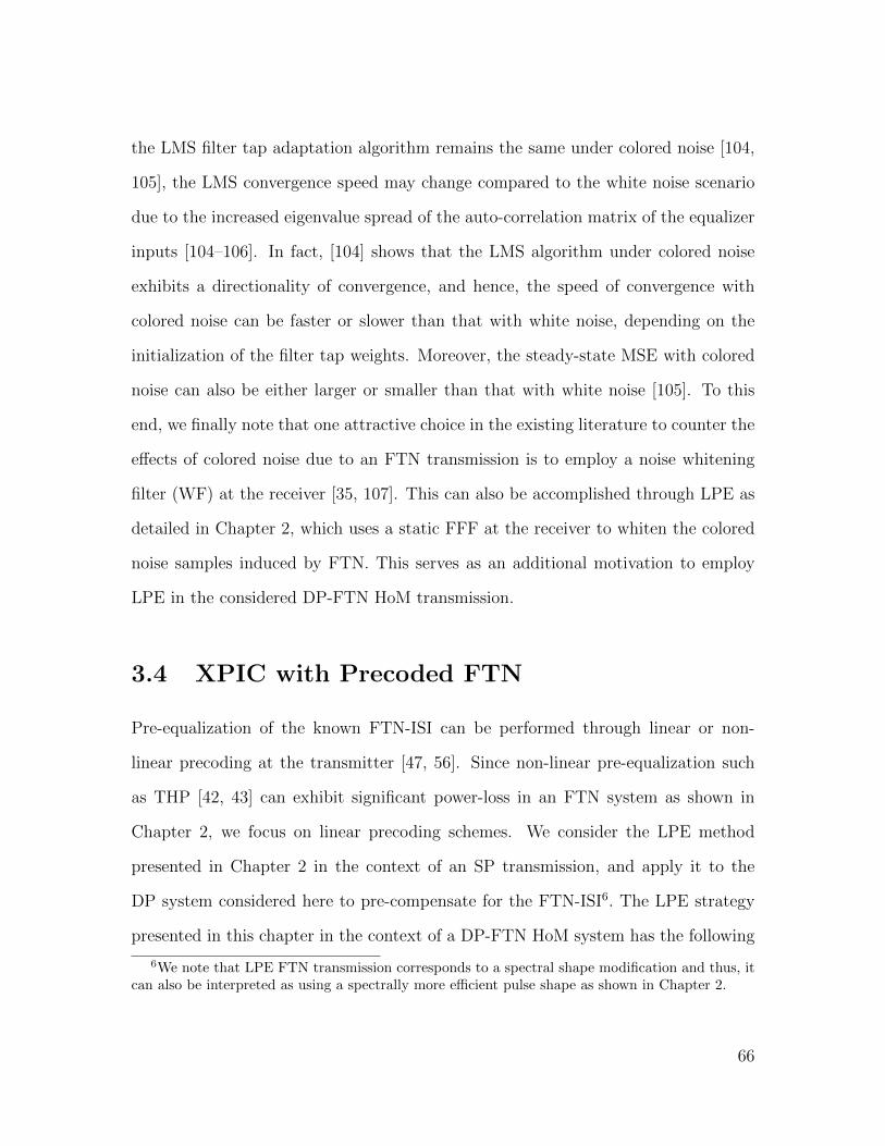
the LMS filter tap adaptation algorithm remains the same under colored noise [104,

105], the LMS convergence speed may change compared to the white noise scenario

due to the increased eigenvalue spread of the auto-correlation matrix of the equalizer

inputs [104–106]. In fact, [104] shows that the LMS algorithm under colored noise

exhibits a directionality of convergence, and hence, the speed of convergence with

colored noise can be faster or slower than that with white noise, depending on the

initialization of the filter tap weights. Moreover, the steady-state MSE with colored

noise can also be either larger or smaller than that with white noise [105]. To this

end, we finally note that one attractive choice in the existing literature to counter the

effects of colored noise due to an FTN transmission is to employ a noise whitening

filter (WF) at the receiver [35, 107]. This can also be accomplished through LPE as

detailed in Chapter 2, which uses a static FFF at the receiver to whiten the colored

noise samples induced by FTN. This serves as an additional motivation to employ

LPE in the considered DP-FTN HoM transmission.

3.4 XPIC with Precoded FTN

Pre-equalization of the known FTN-ISI can be performed through linear or non-

linear precoding at the transmitter [47, 56]. Since non-linear pre-equalization such

as THP [42, 43] can exhibit significant power-loss in an FTN system as shown in

Chapter 2, we focus on linear precoding schemes. We consider the LPE method

presented in Chapter 2 in the context of an SP transmission, and apply it to the

DP system considered here to pre-compensate for the FTN-ISI6. The LPE strategy

presented in this chapter in the context of a DP-FTN HoM system has the following

6We note that LPE FTN transmission corresponds to a spectral shape modification and thus, itcan also be interpreted as using a spectrally more efficient pulse shape as shown in Chapter 2.

66

September

29, 2017

1

+

-LPE

FBF

+

-LPE

FBF

LPE Precoding

𝑎1

𝑎2

DAC

DAC𝑎2

𝑎1

(a) Transmitter

September

29, 2017

1

LP

E

FF

F

LP

E

FF

F

LPE FFF

Rx DSP

(DFE+ CPNT/IPNT)

𝑢1

𝑢2𝑢2

𝑢1

(b) Receiver

Figure 3.6: LPE-FTN DSP, where the shaded blocks represent additional signalprocessing compared to a DFE-FTN system.

differences compared to the LPE proposed in Chapter 2: (a) the inputs to the LPE-

FFF at the DP receiver are corrupted with multi-path ISI, XPI and PN, and (b) LPE-

FBF and LPE-FFF are used in conjunction with the DFE-CPNT and DFE-IPNT

proposed in Section 3.3 of this chapter, which constitutes a combined equalizer and

PN cancellation structure for the DP transmission. As later shown in Section 3.5.3,

this combined structure not only works efficiently, but also outperforms the DFE-only

equalization scheme by significant SNR margins.

Fig. 3.6 illustrates the additional signal processing performed at the transmitter

and receiver of a DP LPE-FTN system compared to an unprecoded transmission. At

the LPE transmitter of Fig. 3.6a, each of the modulated data symbols a1 and a2 is

filtered by a static LPE-FBF bLPE to produce the sequences a1 and a2, respectively,

before the digital-to-analog conversion and pulse-shaping. Similarly, at the LPE

receiver shown in Fig. 3.6b, the received symbols ui, i=1, 2, are filtered by the static

LPE-FFF fLPE to generate the sequences ui. Thereafter, the samples ui, i=1, 2, are

processed by the adaptive 2-D DFE to combat the residual interference and PN.

67

Since the FTN-ISI is perfectly known at the transmitters and receivers for a given

pair of β and τ , the filters bLPE and fLPE can be computed in advance, without any

feedback from the receivers. In addition to converting the effective FTN-ISI into a

minimum-phase impulse response, fLPE also serves the purpose of whitening the noise

samples [44] at the 2-D DFE input. The computational details of the LPE-FBF and

LPE-FFF are relegated to Appendix B.2.

Following the LPE-FFF stage at the receiver, the ISI induced by FTN is com-

pletely eliminated for each polarization. The residual effects of the multipath ISI, XPI

and PN can be subsequently compensated by the LMS-DFE with CPNT or IPNT

method. Numerical results presented in the following section show that the combi-

nation of LPE precoding and an adaptive 2-D DFE at the receiver outperforms a

DFE-only equalization approach. However, as mentioned earlier, LPE-FTN modifies

the spectral shape as shown in the previous chapter.

Finally, we remark that for the FTN equalization methods proposed in Sections 3.3

and 3.4 in this chapter, we consider DFE and linear precoding, which rely on the spec-

tral factorization [44] of the overall FTN-ISI channel, stemming from the transmitter

pulse-shape and the receiver matched filter. When τ < 11+β

, the presence of uncount-

ably many spectral zeros makes such factorization unrealizable as shown in Chapter 2.

Therefore, similar to the LPE in Chapter 2 and the precoding method in [47], for our

current work, we assume the following relation between β and τ :

τ ≥ 1

1 + β. (3.35)

While this restriction limits τ to be slightly above the Mazo limit [7, 8] corresponding

to the same minimum-distance for a given β, the limiting value τ = 11+β

by itself is

significantly meaningful as this choice of τ maximizes the FTN capacity [108].

68

3.5 Numerical Results and Discussion

In this section, we illustrate and validate the proposed methods by way of numer-

ical simulations. Due to absence of previous works on DP-FTN HoM systems, we

benchmark the error-rate performances of the proposed methods against Nyquist

transmissions in the presence and absence of PN distortions.

3.5.1 Simulation Setup

For the simulations, we consider the discrete-time baseband DP-FTN HoM microwave

communication system shown in Fig. 3.2. FEC coding, modulation and FTN param-

eters for both polarization branches are kept identical for evaluating the average

performance of the DP system. For our simulations, we use an LDPC code7 with

rate 0.9 and codeword length 64800 bits, a random bit-interleaver, 256, 512 and

1024-QAM formats, and different FTN acceleration factors τ for the DP-FTN trans-

missions. As the roll-off factors of the RRC filters in practical microwave systems

can generally vary from 0.25 [25] to 0.5 [24, 27, 111], we have chosen β = 0.25, 0.3

and 0.4 for presenting our results. We consider a 23 Mbaud Nyquist symbol rate for

each polarization, which is effectively 23τ

Mbaud with FTN signaling for the same

bandwidth [13].

To simulate the Wiener PN processes, we have considered equal contributions

of PN due to the transmitter and receiver LOs, such that σwti= σwri , and σ∆ =√σ2wti

+σ2wri

= 0.13◦ [30, 31], i= 1, 2, corresponding to a PN level of −95 dBc/Hz at

100 kHz offset from the center frequency for a 23 Mbaud symbol rate as in [32, 99].

7The code is compliant with the second generation digital video broadcasting standard for satel-lite (DVB-S2) applications [109, 110], and this is encoded as an irregular repeat accumulate (IRA)code. LDPC decoding is performed by iterative standard message passing algorithm [110], with themaximum number of LDPC internal iterations set to 50.

69

The multipath reflections and XPI, which are assumed to be unknown to the

transmitters and receivers, are simulated as a 2×2 ISI channel matrix similar to [27].

The matrix elements are modeled by Rummler’s well-known fixed-delay, two-ray

model [61], such that the frequency response of each element of the channel matrix

can be written as a function of frequency f as

Sij(f)=aij

[1−10−

dN,ij20 ej2π(f−fN,ij)τ0

], i, j∈{1, 2}. (3.36)

In (3.36), dN,ij is the notch-depth set to 5 dB and 3 dB for i=j and i 6=j, respectively,

fN,ij is the notch-frequency set to 10 MHz and 7 MHz for i=j and i 6=j, respectively,

τ0 = 6.3 ns is a fixed-delay, and aij is a gain constant normalized to produce unit

energy co-polarization channels when i= j and a 15 dB attenuation for i 6= j, such

that the DP-system has a 15 dB cross-polarization discrimination (XPD) value as

in [26, 32].

We consider a 15-tap FFF and a 11-tap FBF for the adaptive DFE. An initial

amount of pilot symbols are inserted at the beginning of transmission to ensure LMS

convergence, during which the adjustable filter tap-coefficients converge to nearly

stationary values as in [75, 102]. Thereafter, four QPSK training symbols, with

the same average power as the data symbols, are transmitted after every 200 data

symbols for each polarization, causing a 2% pilot-transmission overhead [30]. The

adaptive LMS-DFE switches between training and decision-directed modes across

the blocks of pilots and data transmission, respectively. Similar to [75], the step-

size parameters associated with the DFE filter tap-weights are chosen to be smaller

than those of the PN-estimators to account for faster time-variation of carrier phases

over the multipath channel, and their values, together with the decision delay k0,

are optimized to minimize the steady-state MSE. For the DP LPE-FTN system,

70

additional static FBFs and FFFs with 12 and 15 taps, respectively, are applied at the

transmitters and receivers of both polarizations as described in Section 3.4. Following

equalization and PN mitigation, soft-demapping is performed on the DFE-outputs

and the LLRs are passed on to the LDPC decoder.

For the subsequent performance analyses in this section, we consider the DP-

Nyquist and the DP-FTN transmissions with the same average transmit power. The

error-rate simulations and the SEs of different systems are evaluated as a function of

SNR, which for the ith polarization data stream, i=1, 2, is computed from (3.3) as

SNR =E(|si[k]|2)

σ2ni

, (3.37)

where E(·) denotes the expectation operator and si is the signal component of the

received samples ui in (3.3), i=1, 2, such that

si[k] = ejθri [k]

2∑j=1

∑l

rj[k−l]ejθtj [k−l]hij[l] , (3.38)

where the sequences rj, j = 1, 2, correspond to the modulated symbols aj for the

unprecoded systems, and the precoded symbols aj for the LPE precoded FTN trans-

missions, respectively.

3.5.2 Performance with DFE-FTN

We first investigate the efficiency of the proposed algorithms by conducting the follow-

ing two performance comparisons: (a) CPNT vs. IPNT method, and (b) DP-Nyquist

vs. DP-FTN transmissions. For this, we consider the adaptive DFE with the PN

mitigation techniques presented in Section 3.3. Fig. 3.7 shows the coded BER per-

formance measured after the LMS convergence. For the computer simulations, 300

71

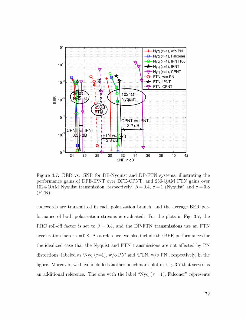
24 26 28 30 32 34 36 38 40 4210

−6

10−5

10−4

10−3

10−2

10−1

100

SNR in dB

BE

R

1024QNyquist

CPNT vs IPNT 3.2 dB

256QNyquist

256QFTN

CPNT vs IPNT 0.55 dB FTN vs. Nyq

3.3 dB

Nyq (τ=1), w/o PN

Nyq (τ=1), Falconer

Nyq (τ=1), IPNT100

Nyq (τ=1), IPNT

Nyq (τ=1), CPNT

FTN, w/o PN

FTN, IPNT

FTN, CPNT

Figure 3.7: BER vs. SNR for DP-Nyquist and DP-FTN systems, illustrating theperformance gains of DFE-IPNT over DFE-CPNT, and 256-QAM FTN gains over1024-QAM Nyquist transmission, respectively. β = 0.4, τ = 1 (Nyquist) and τ = 0.8(FTN).

codewords are transmitted in each polarization branch, and the average BER per-

formance of both polarization streams is evaluated. For the plots in Fig. 3.7, the

RRC roll-off factor is set to β = 0.4, and the DP-FTN transmissions use an FTN

acceleration factor τ=0.8. As a reference, we also include the BER performances for

the idealized case that the Nyquist and FTN transmissions are not affected by PN

distortions, labeled as ‘Nyq (τ=1), w/o PN’ and ‘FTN, w/o PN’, respectively, in the

figure. Moreover, we have included another benchmark plot in Fig. 3.7 that serves as

an additional reference. The one with the label “Nyq (τ = 1), Falconer” represents

72

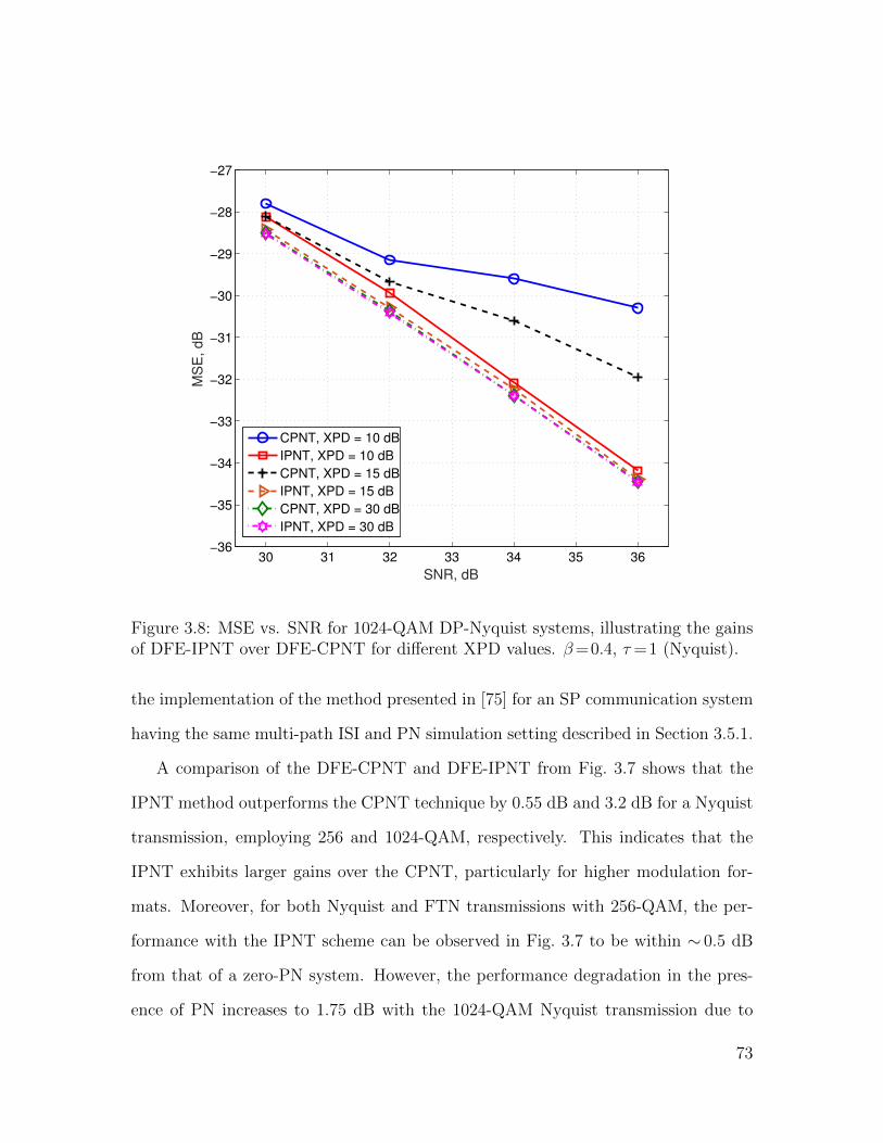
30 31 32 33 34 35 36−36

−35

−34

−33

−32

−31

−30

−29

−28

−27

SNR, dB

MS

E, dB

CPNT, XPD = 10 dB

IPNT, XPD = 10 dB

CPNT, XPD = 15 dB

IPNT, XPD = 15 dB

CPNT, XPD = 30 dB

IPNT, XPD = 30 dB

Figure 3.8: MSE vs. SNR for 1024-QAM DP-Nyquist systems, illustrating the gainsof DFE-IPNT over DFE-CPNT for different XPD values. β=0.4, τ=1 (Nyquist).

the implementation of the method presented in [75] for an SP communication system

having the same multi-path ISI and PN simulation setting described in Section 3.5.1.

A comparison of the DFE-CPNT and DFE-IPNT from Fig. 3.7 shows that the

IPNT method outperforms the CPNT technique by 0.55 dB and 3.2 dB for a Nyquist

transmission, employing 256 and 1024-QAM, respectively. This indicates that the

IPNT exhibits larger gains over the CPNT, particularly for higher modulation for-

mats. Moreover, for both Nyquist and FTN transmissions with 256-QAM, the per-

formance with the IPNT scheme can be observed in Fig. 3.7 to be within ∼ 0.5 dB

from that of a zero-PN system. However, the performance degradation in the pres-

ence of PN increases to 1.75 dB with the 1024-QAM Nyquist transmission due to

73

enhanced vulnerability of higher modulation orders to PN impairments. Addition-

ally, we also notice from Fig. 3.7 that when the XPI is negligibly small with an

XPD value of 100 dB, the adaptive DFE-IPNT method, indicated by the label “Nyq

(τ = 1), IPNT100” is able to achieve similar BER performance as that of the SP

transmission.

To perform a more comprehensive comparison between the IPNT and CPNT

methods, we recall from Section 3.3 that the gains of DFE-IPNT over DFE-CPNT

increase for higher modulation orders as the XPI grows stronger, i.e. for smaller

values of XPD [26, 32]. We verify this claim in Fig. 3.8 by plotting the steady-state

MSE averaged over the two polarization data streams as a function of SNR, for a 1024-

QAM DP-Nyquist transmission with varying XPD values. As shown in Fig. 3.8, both

IPNT and CPNT yield similar MSEs for milder XPI when XPD = 30 dB. However,

as the cross-talk between the two orthogonal polarizations increases, the MSE for

IPNT shows significant improvement over CPNT. When the XPI is severe with XPD

= 10 dB, the average MSE with the DFE-IPNT scheme can be seen to be 4 dB lower

compared to that of the DFE-CPNT at an SNR of 36 dB.

We now proceed to analyze the performance difference between Nyquist and FTN

signaling. For this, we first compare the BER of a 256-QAM Nyquist system with

that of a 256-QAM FTN transmission. Fig. 3.7 shows that employing the same

modulation order and the DFE-IPNT method, the DP-FTN system offers a 25%

increase in the data rate, corresponding to an FTN acceleration factor 0.8, over the

DP-Nyquist system at the price of a 3.5 dB SNR penalty. Additionally, in Fig. 3.7,

we also perform a comparison between a 1024-QAM Nyquist system and a 256-QAM

FTN transmission having τ = 0.8, such that both systems achieve the same data

rate. For example, with a 23 Mbaud Nyquist symbol rate and a LDPC code rate of

74

26 28 30 32 34 3610

−6

10−5

10−4

10−3

10−2

10−1

SNR in dB

BE

R

256QNyquist

2.2 dBPrecoding vs. no−precoding

β = 0.3

1024QNyquist

256QLPE

256QDFE

3.6 dBFTN vs. Nyq

5.5 dBFTN vs. Nyq

256Q Nyq (τ = 1), IPNT

256Q LPE, CPNT

256Q LPE, IPNT

256Q DFE, IPNT

256Q DFE, CPNT

256Q DFE, IPNT, 30 FFF

1024Q Nyq (τ = 1), IPNT

Figure 3.9: BER vs. SNR for DP-FTN systems, illustrating the performance gainsof LPE-FTN over DFE-FTN. 256 and 1024-QAM, β = 0.3, 0.4, τ = 1 (Nyquist) andτ=0.8 (FTN).

0.9, both DP systems employing different modulation schemes yield a data rate of

414 Mbits/sec. Fig. 3.7 highlights a performance gain of 3.3 dB for the 256-QAM FTN

system over the 1024-QAM Nyquist transmission. This suggests that in the presence

of PN, with the DFE-IPNT method, a DP-FTN system can significantly outperform

a DP-Nyquist transmission that uses a higher modulation format to produce the same

data rate.

However, the adaptive DFE described in Section 3.3 needs to equalize the com-

bined ISI due to multipath propagation and FTN. As we shall observe in the following,

the BER performance of the DP-FTN transmission can be further improved by elimi-

75

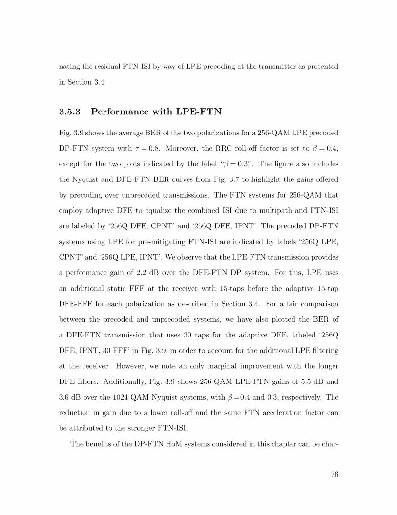
nating the residual FTN-ISI by way of LPE precoding at the transmitter as presented

in Section 3.4.

3.5.3 Performance with LPE-FTN

Fig. 3.9 shows the average BER of the two polarizations for a 256-QAM LPE precoded

DP-FTN system with τ = 0.8. Moreover, the RRC roll-off factor is set to β = 0.4,

except for the two plots indicated by the label “β = 0.3”. The figure also includes

the Nyquist and DFE-FTN BER curves from Fig. 3.7 to highlight the gains offered

by precoding over unprecoded transmissions. The FTN systems for 256-QAM that

employ adaptive DFE to equalize the combined ISI due to multipath and FTN-ISI

are labeled by ‘256Q DFE, CPNT’ and ‘256Q DFE, IPNT’. The precoded DP-FTN

systems using LPE for pre-mitigating FTN-ISI are indicated by labels ‘256Q LPE,

CPNT’ and ‘256Q LPE, IPNT’. We observe that the LPE-FTN transmission provides

a performance gain of 2.2 dB over the DFE-FTN DP system. For this, LPE uses

an additional static FFF at the receiver with 15-taps before the adaptive 15-tap

DFE-FFF for each polarization as described in Section 3.4. For a fair comparison

between the precoded and unprecoded systems, we have also plotted the BER of

a DFE-FTN transmission that uses 30 taps for the adaptive DFE, labeled ‘256Q

DFE, IPNT, 30 FFF’ in Fig. 3.9, in order to account for the additional LPE filtering

at the receiver. However, we note an only marginal improvement with the longer

DFE filters. Additionally, Fig. 3.9 shows 256-QAM LPE-FTN gains of 5.5 dB and

3.6 dB over the 1024-QAM Nyquist systems, with β=0.4 and 0.3, respectively. The

reduction in gain due to a lower roll-off and the same FTN acceleration factor can

be attributed to the stronger FTN-ISI.

The benefits of the DP-FTN HoM systems considered in this chapter can be char-

76

22 24 26 28 30 32 334

6

8

10

12

SNR in dB

SE

(bits/s

/Hz/p

ol.)

Constrained Cap., w/o PN and XPI

Nyquist (τ = 1)

DFE−FTN

LPE−FTN

1024Q

β = 0.4

1024Q

β = 0.3

512Q

β = 0.25256Q

β = 0.4,

τ = 0.8

β = 0

β = 0.3

β = 0.4

256Q β = 0.3, τ = 0.8

β = 0.25

256Q

β = 0.25, τ = 0.89

256Q

β = 0.25

256Q

β = 0.4

Figure 3.10: Spectral efficiency vs. SNR for DP-Nyquist and DP-FTN schemes. 256,512 and 1024-QAM, β=0.25, 0.3 and 0.4, τ=1 (Nyquist) and τ=0.8, 0.89 (FTN).

acterized by the SE improvements they provide. The SE value for the ith polarization

data stream, i= 1, 2, with the RRC roll-off β, FTN factor τ , modulation order Mi,

and a code-rate Ri, can be written as

SE =Ri log2(Mi)

(1 + β)τbits/sec/Hz/polarization . (3.39)

Fig. 3.10 shows the SE achieved, per polarization, by the proposed DP-HoM sys-

tems as a function SNR, with different values of β and τ . The required SNR to

attain a given SE corresponds to an average BER of 10−6 for the respective systems.

In Fig. 3.10, we have also included the normalized constrained capacities [108] corre-

77

sponding to different roll-off factors in an SP transmission without PN, as a reference.

We note that the normalized capacity with β=0 is superior to those of the other RRC

pulse-shapes having β > 0 [108]. As observed from the SE values in the figure, for

example, a 256 and a 1024-QAM Nyquist transmission correspond to 5.14 and 6.43

bits/sec/Hz/polarization, respectively, with β = 0.4, and LDPC code rate 0.9. The

SE figures improve with decreasing filter bandwidths as shown for the RRC roll-offs

0.25 and 0.3. We note that by using the FTN factors 0.8 and 0.89, a 256-QAM FTN

system can achieve the same SE as a 1024-QAM and a 512-QAM Nyquist trans-

mission, respectively. In Fig. 3.10, the comparison between the Nyquist and FTN

systems that yield the same SE shows that a 256-QAM DP-FTN system with τ=0.8,

using IPNT PN mitigation method and LPE precoding, can demonstrate a 5.5 dB

SNR advantage compared to the 1024-QAM Nyquist system for β = 0.4. Similarly,

a 256-QAM DP LPE-FTN system with τ = 0.89 outperforms a 512-QAM Nyquist

system by an SNR margin of 2.9 dB for β=0.25. Moreover, the 256-QAM precoded

FTN systems with different τ values can be seen to offer a 12−25% higher SE than

the 256-QAM Nyquist signaling with a 0.7−3.2 dB SNR penalty.

Next, we show the PN tolerance of different modulation schemes employing the

proposed methods with varying PN intensities. In Fig. 3.11, we have plotted the

additional SNR required over the respective ideal systems that are not affected by

PN distortions, to attain a coded BER of 10−6, for each value of σ∆ defined in

Section 3.5.1. The figure suggests that lower modulation orders offer higher tolerance

to PN distortions. For example, when σ∆ =0.2◦, 512 and 1024-QAM Nyquist systems

show 0.7 dB and 2.9 dB additional SNR penalty from the respective zero-PN reference

systems compared to a 256-QAM system. Moreover, at the same SNR distance, e.g.

1 dB from the corresponding zero-PN reference systems, 256-QAM and 512-QAM DP

78

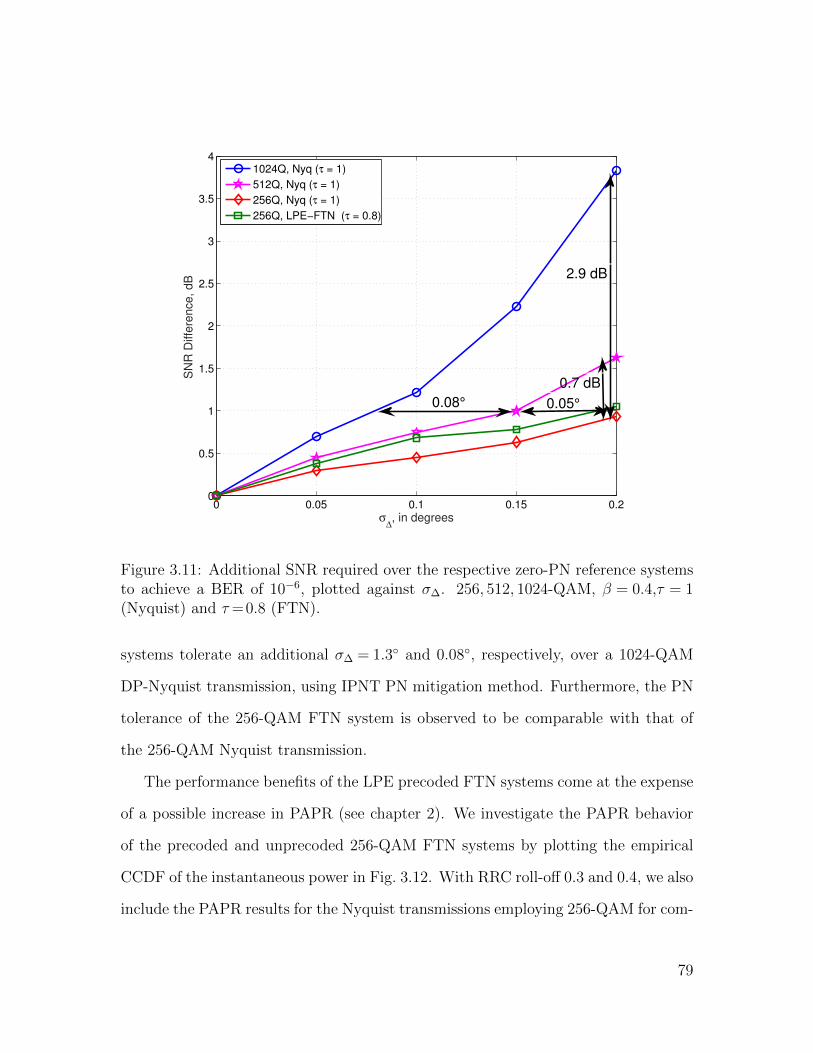
0 0.05 0.1 0.15 0.20

0.5

1

1.5

2

2.5

3

3.5

4

σ∆, in degrees

SN

R D

iffe

rence, dB

0.08° 0.05°

2.9 dB

0.7 dB

1024Q, Nyq (τ = 1)

512Q, Nyq (τ = 1)

256Q, Nyq (τ = 1)

256Q, LPE−FTN (τ = 0.8)

Figure 3.11: Additional SNR required over the respective zero-PN reference systemsto achieve a BER of 10−6, plotted against σ∆. 256, 512, 1024-QAM, β = 0.4,τ = 1(Nyquist) and τ=0.8 (FTN).

systems tolerate an additional σ∆ = 1.3◦ and 0.08◦, respectively, over a 1024-QAM

DP-Nyquist transmission, using IPNT PN mitigation method. Furthermore, the PN

tolerance of the 256-QAM FTN system is observed to be comparable with that of

the 256-QAM Nyquist transmission.

The performance benefits of the LPE precoded FTN systems come at the expense

of a possible increase in PAPR (see chapter 2). We investigate the PAPR behavior

of the precoded and unprecoded 256-QAM FTN systems by plotting the empirical

CCDF of the instantaneous power in Fig. 3.12. With RRC roll-off 0.3 and 0.4, we also

include the PAPR results for the Nyquist transmissions employing 256-QAM for com-

79

−2 0 2 4 6 810

−4

10−3

10−2

10−1

100

Inst. Power (dBW)

Pro

b (

Inst. P

ow

er

> A

bscis

sa)

Unprecoded Nyq, β = 0.4

Unprecoded FTN, β = 0.4

LPE−FTN, β = 0.4

Unprecoded Nyq, β = 0.3

Unprecoded FTN, β = 0.3

LPE−FTN, β = 0.3

Figure 3.12: Empirical CCDF of the instantaneous power with average transmitpower = 0 dBW. 256-QAM, β=0.3 and 0.4, τ=1 (Nyquist) and τ=0.8 (FTN).

parison. All transmission schemes are normalized to the same average transmitted

power of 0 dBW, such that the ‘X-axis’ spread to the right hand side of the X=0 dBW

line determines the deviation of the peak power from the average power, i.e. PAPR,

with the corresponding probability shown along the ‘Y-axis’. Fig. 3.12 suggests that

FTN signaling can exhibit a 0.75−0.9 dB higher PAPR than the Nyquist transmission

at a CCDF value 10−4. Moreover, PAPR with an FTN transmission increases slightly

with smaller RRC roll-off factors as FTN-ISI grows stronger. However, as seen in the

figure, the LPE-precoded FTN systems yield only a marginally higher PAPR than

80

Table 3.1: Computational Complexities: CPNT vs. IPNT

Operation CPNT IPNTComplex Addition/Subtraction 8Nf +4Nb+4=168 12Nf +8Nb+16=284

Complex Multiplication/Division 12Nf +4Nb+16=240 24Nf +8Nb+24=472Total Complex Calculations 408 756

Hard Symbol-Decisions 2 2

the unprecoded FTN transmissions8.


In this section, we present an analysis of the computational cost for the proposed

CPNT and IPNT methods. The number of the mathematical operations needed

during every symbol period of the DP transmission is furnished in Table 3.1 as a

function of Nf and Nb. To illustrate this analysis with further clarity and ease of

comparison, a specific example, corresponding to our simulation setting Nf =15 and

Nb =11, is also provided. The numbers in Table 3.1 reveal that the implementation

complexity to update the IPNT estimates according to (3.23)-(3.30) is slightly higher

than that of the CPNT adaptation given in (3.7)-(3.12), at the cost of a significantly

superior BER performance demonstrated in Section 3.5.2. Moreover, Table 3.1 shows

that the LMS adaptation in the decision-directed mode performs two hard symbol

decisions for the employed QAM constellation. The table entries also reveal that the

number of complex calculations required for the PN and equalizer-taps adaptation

does not depend on the modulation order. Therefore, our proposed methods show

ease of scalability with higher modulation formats.

8We remark that the consideration of PAPR reduction schemes, such as [112] for FTN trans-mission, and their operation in tandem with pre-distortion methods usually applied for microwavesystems using HoM, is an interesting extension to mitigate and analyze the effects of PAPR increase.

81

3.6 Conclusions

A synchronous DP-FTN HoM transmission is an attractive choice to increase the SE

in fixed wireless backhaul links. However, the SE improvements offered by such a

system comes at the expense of introducing ISI, XPI and vulnerability to PN. Us-

ing FTN signaling in a DP transmission can moderate the need for adopting very

high modulation orders that are more sensitive to PN distortions. In this chap-

ter, DP-FTN HoM systems have been investigated for the first time. In order to

equalize interference and recover carrier phase, we proposed a joint XPIC and PN

compensation scheme coupled with an adaptive LMS-DFE. The ISI induced by FTN

is mitigated either through the LMS-DFE at the receiver or linear pre-equalization at

the transmitter. Numerical results for a microwave radio transmission show that an

FTN signaling with the proposed interference mitigation schemes can exhibit as high

as 3−5.5 dB performance improvement over a Nyquist transmission that employs a

higher modulation order to achieve the same data rate. Alternatively, for a given

modulation scheme, a DP-FTN signaling can offer a 12−25% SE enhancement over

a DP-Nyquist signaling with a 0.7−3.2 dB SNR degradation.

82

Chapter 4

Multicarrier Faster-than-Nyquist

Optical Transmission

4.1 Introduction

OFC system is a suitable platform for the introduction of FTN signaling, since con-

ventional SE improvement means, such as employing HoM formats, are challenging

for such a system. In Chapter 2, we have considered single carrier optical fiber trans-

mission using FTN signaling. However, such systems are restrictive in achieving very

high data rates, because the practical limitations of the opto-electronics preclude

the feasibility of increasing the baud rate beyond a certain value. Therefore, MFTN

transmission using TFP WDM superchannels [10, 11, 13, 17, 80, 113, 114] is an at-

tractive choice to achieve high data rates in OFC systems. Such a benefit of the TFP

transmission comes at the price of introducing ISI and ICI. Therefore, enjoying the

SE benefits of the TFP systems entails successful mitigation of such interference.

Alternative to the high-complexity equalization strategies, we investigate pre-

coding techniques in this chapter, as an extension to the pre-equalization method

presented in Chapter 2. Since the well-known THP incurs significant precoding loss

and modulo-loss [44], particularly with FTN signaling (see Chapter 2), we consider

linear precoding, similar to Chapter 2. However, different from the ISI-only systems

considered in Chapter 2, we need to mitigate both ISI and ICI in this chapter. This

83

thesis is the first to consider precoding in MFTN systems that employ packing of

symbols in both time and frequency dimensions.

For our first contribution, we present a new 2-D linear LPE technique, as an

extension of the 1-D LPE proposed in Chapter 2. By orthogonalizing the FTN trans-

mission through joint filtering of the constituent SCs of an MFTN system, 2-D LPE

yields optimal error-rate performance, which makes it competitive to computation-

ally prohibitive and buffer-space constrained BCJR based equalization algorithms.

However, such a precoding method is restrictive in terms of the time and frequency

compression achievable in an MFTN transmission. To address this problem, as a sec-

ond contribution, we propose a sub-optimal partial precoding strategy, which facili-

tates transmitter-side 1-D LPE precoding for the individual SCs of the TFP system,

followed by a receiver-side turbo ICI cancellation. We validate the advantages of

our proposed precoding schemes over the existing TFP interference mitigation meth-

ods, through numerical simulations of a coherent TFP optical WDM superchannel

transmission, which has attracted significant attention more recently [11, 17, 114].

The remainder of the chapter is organized as follows. The system model is intro-

duced in Section 4.2. In Section 4.3, we propose two precoding strategies to counter

TFP ISI and ICI. Section 4.4 demonstrates the benefits of our proposals through

simulations. Finally, Section 4.5 provides concluding remarks.

4.2 System Model

We consider the baseband system model for precoded MFTN transmission under an

AWGN channel shown in Fig. 4.1. For each kth SC, k∈1, 2, · · · , N , with N being the

total number of SCs, an LDPC coded and modulated data stream ak is either jointly

or separately precoded by a linear FBF. The precoded signal dk is then frequency

84

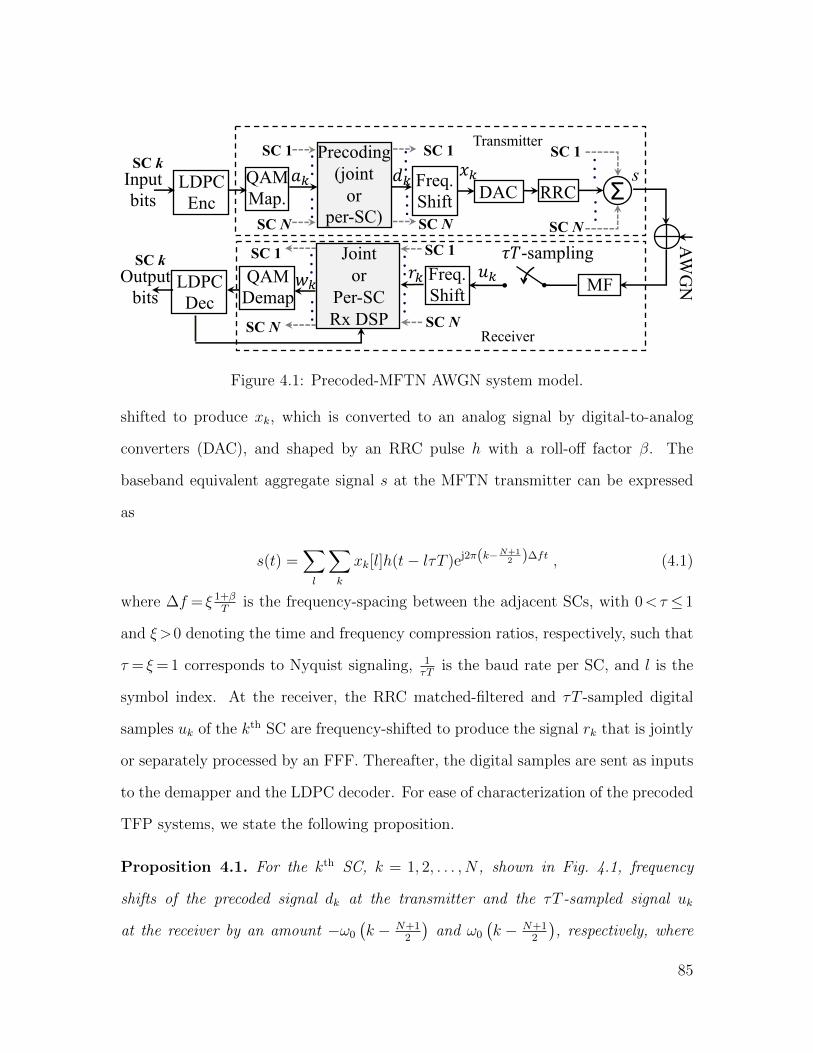
SC N

Input bits

LDPCEnc

QAMMap. DAC

...

...

SC 1SC k

Σ

Precoding(joint

orper-SC)

RRC

...

...

SC 1

SC N

Freq.Shift

Joint or

Per-SCRx DSP

MF

!"-samplingFreq.Shift

...

...

SC 1

SC NSC N

LDPCDec

QAMDemap

...

...

SC 1Output

bits

SC k

AWG

NTransmitter

Receiver

#$ s%$

&$'$

($

)$

SC N

...

...

SC 1

Figure 4.1: Precoded-MFTN AWGN system model.

shifted to produce xk, which is converted to an analog signal by digital-to-analog

converters (DAC), and shaped by an RRC pulse h with a roll-off factor β. The

baseband equivalent aggregate signal s at the MFTN transmitter can be expressed

as

s(t) =∑l

∑k

xk[l]h(t− lτT )ej2π(k−N+12 )∆ft , (4.1)

where ∆f = ξ 1+βT

is the frequency-spacing between the adjacent SCs, with 0<τ ≤ 1

and ξ>0 denoting the time and frequency compression ratios, respectively, such that

τ = ξ= 1 corresponds to Nyquist signaling, 1τT

is the baud rate per SC, and l is the

symbol index. At the receiver, the RRC matched-filtered and τT -sampled digital

samples uk of the kth SC are frequency-shifted to produce the signal rk that is jointly

or separately processed by an FFF. Thereafter, the digital samples are sent as inputs

to the demapper and the LDPC decoder. For ease of characterization of the precoded

TFP systems, we state the following proposition.

Proposition 4.1. For the kth SC, k = 1, 2, . . . , N , shown in Fig. 4.1, frequency

shifts of the precoded signal dk at the transmitter and the τT -sampled signal uk

at the receiver by an amount −ω0

(k − N+1

2

)and ω0

(k − N+1

2

), respectively, where

85

...!"

!#.

!$

2D LPEFFF% ....

...

&"

&#

&$

......

2D LPEFBF '

("(#

.

($ Σ.........

............

......

)")#)$+ -

(a) Transmitter

!"

!#.

!$

2D LPEFBF% ....

...

&"

&#

&$

......

'"

'#.

'$

2D LPEFFF( ....

...

)"

)#

)$

......

(b) Receiver

Figure 4.2: 2-D LPE, where the shaded blocks represent additional signal processingcompared to unprecoded MFTN systems.

ω0 =2π∆fτT , translates the overall TFP channel into a linear time-invariant (LTI)

system, and the z-transform H(z) of the corresponding 2-D channel response is a

Hermitian matrix polynomial.

Proof. See Appendix C.1.

4.3 Precoding Solutions

4.3.1 Joint precoding: 2-D LPE

Schematics of the 2-D LPE are shown in Fig. 4.2a-4.2b corresponding to the trans-

mitter and receiver filtering operations, respectively. In Fig. 4.2a, the modulated

data symbols ak, k = 1, 2, . . . , N from all SCs are jointly processed by a linear 2-

D FBF B to produce the precoded symbols dk, translating the overall precoding

operation into an effective IIR filter. The minimum-phase property of the FBF guar-

antees the stability of the IIR operation [44]9. At the receiver shown in Fig. 4.2b, the

frequency-shifted symbols rk, k=1, 2, . . . , N from all SCs are further jointly processed

by a linear 2-D FFF F , which whitens the colored noise caused by FTN sampling.

9We remark that different from a conventional ISI channel, such linear IIR filtering does notinduce a precoding loss in an FTN system (see Chapter 2), since the MFTN “channel” is part ofthe transmitter.

86

Thereafter, the filtered samples are sent as inputs to a symbol-by-symbol demapper.

Inspired by [115], the FFF and the FBF matrix computation from the 2-D channel

matrix H defined in Proposition 4.1 is summarized below.

Proposition 4.2. With the Cholesky decomposition of the Hermitian matrix polyno-

mial H(z) performed as

H(z) = V (z)V H(z−∗), (4.2)

where V (z)=∑k≥0

Vkz−k is causal and minimum-phase, i.e., Vk=0 for k<0, V (z) is

nonsingular for |z| ≥ 1 and V0 is lower triangular, the 2-D LPE FFF and FBF are

given by

F (z) = D−1JV −1(z−∗)J , (4.3)

B(z) = D−1JV H (z∗)J , (4.4)

respectively, with J being the K×K anti-diagonal identity matrix, K is the number of

TFP-channel taps, (·)∗ represents the complex conjugate of a complex scalar, (·)−∗ =

1(·)∗ , [·]H and [·]−1 denote the matrix Hermitian and matrix inverse, respectively, D =

diag(v∗0,K,K , · · · , v∗0,1,1

), v0,i,j are the ith and jth entries of V0, and diag(· · · ) denotes

the diagonal matrix constructed with the specified elements.

Proof. See Appendix C.2.

By converting the MFTN transmission into an orthogonal system similar to the

LPE method in Chapter 2, 2-D LPE yields optimal error-rate performance without

performing any iterations between the equalizer and the LDPC decoder. However,

such precoding suffers from the following two drawbacks: (a) for the joint filtering

across SCs, it requires access to the digital samples of all SCs at both the transmitter

87

!"1D LPE FBF #$

%&

%".

%'

1D LPE FFF()

....

...

*&

*"

*'

......1D LPE FFF

()1D LPE FFF

()

PIC

LDPCDec

LDPCDec

LDPCDec

+&

+".

+'...

...Σ

!'1D LPE FBF #,

Σ

!&1D LPE FBF #-

Σ...

......

....&

."

.'

+ -

+ -

+ -

(a) Transmitter

!"1D LPE FBF #$

%&

%".

%'

1D LPE FFF()

....

...

*&

*"

*'

......1D LPE FFF

($1D LPE FFF

(+

PIC

LDPCDec

LDPCDec

LDPCDec

,&

,".

,'...

...Σ

!'1D LPE FBF #+

Σ

!&1D LPE FBF #)

Σ...

......

...-&

-"

-'

+ -

+ -

+ -

(b) Receiver

Figure 4.3: Partial precoding, where the shaded blocks represent additional signalprocessing compared to unprecoded MFTN systems.

and the receiver, which precludes the realization of independent SC processing, and

(b) 2-D LPE is feasible only for a restricted range of τ, ξ pairs for a given β, since

orthogonalizing the MFTN transmission requires that the net symbol rate is lower

than the aggregate TFP bandwidth, and therefore,

N

(1 + β)τ [(N − 1)ξ + 1]≤1 . (4.5)

Moreover, we also note that the computation of B and F requires the factoriza-

tion (4.2) that is possible if the following Paley-Wiener condition (see e.g. [44, 116])

is satisfied

τT

∫ 12τT

− 12τT

∣∣∣ log det(H(ej2πfτT

)) ∣∣∣df <∞ . (4.6)

To address such limitations of the 2-D LPE, we propose another precoding strategy

as follows.

88

ICI Est.𝐼+,%,+

+ Σ-

-LDPC Dec

bits out 𝑖𝑡 = 𝑖𝑡234

LLR789.𝑖𝑡 < 𝑖𝑡234

LLR toSoft Sym

ICI Est.𝐼+,+,%ICI Est.𝐼+,+;%

ICI Est.𝐼+;%,+

...

...SC 𝑘 − 1

SC 𝑘 + 1

𝑧+ 𝑤+

Figure 4.4: ICI mitigation through PIC.

4.3.2 Partial Precoding (PP)

PP encapsulates a conceptual combination of transmitter-side pre-equalization and

receiver-side equalization of TFP interference, as shown in Fig. 4.3a-4.3b. In order to

pre-mitigate the MFTN-ISI, PP employs separate 1-D LPE FBFs and FFFs for each

SC, at the transmitter and receiver, respectively. For this, the FFFs and FBFs are

computed based on the spectral factorization of the diagonal entries of the channel

response H(z) (see Chapter 2 and Chapter 3 for the computational details). There-

after, the MFTN-ICI is mitigated at the receiver through an iterative PIC approach

in a turbo fashion as detailed in Fig. 4.4, similar to [13, 80, 117].

As shown in Fig. 4.4, PIC enables the extrinsic LLRs fed back from the LDPC

decoders to estimate and cancel the soft-estimates of the ICI stemming from the

adjacent SCs, iteratively. For example, each LDPC iteration uses the extrinsic LLRs

from the (k−1)th and (k+1)th SCs to compute the soft estimates of the data symbols

corresponding to the neighboring SCs [117]. Next, the soft-estimates Ik−1,k and Ik+1,k

are computed and subtracted from the 1-D LPE FFF output symbols zk of the kth

89

SC N

X-pol LDPC Enc

QAMMap.

RRC

Opt. Front-endY-pol QAM

Map.RRC

WD

M

...

...

SC 1

SC k

Coh

. Rx

SSMFDACDAC

IQ

DACDAC

IQ

ADCADC

IQ

ADCADC

IQ

MF+CD Eq.

Other SCs X-pol

2D LPE/Partial

Precoding

Other SCs Y-pol

2D LPE/Partial

Precoding

Other SCs X-pol

Other SCs Y-pol

FreqShift

FreqShift

SC k

MF+CD Eq.

2x2PMDFSE

LDPC Enc

Freq Shift+1D/2D

FFFper Pol.

ToLDPCDec

!",$

!",%

&",$

&",%

Other SCs X-pol

Other SCs Y-pol

Figure 4.5: Simulated MFTN system model: precoded DP TFP WDM optical su-perchannel transmission.

SC, where Ii,j denotes the ICI from the ith SC to the jth SC, i, j∈1, 2, · · · , N .

While PIC is well investigated in the FTN literature as a means to counter ICI, in

this work, we apply it for the first time in tandem with precoding. With this design,

PP based TFP systems completely eliminate the MFTN-ISI without performing com-

putationally challenging BCJR iterations, and can also offer significant performance

advantage over unprecoded PIC-only ISI and ICI equalization approach, such as [80].

We validate this claim through numerical simulations in Section 4.4. We remark that

for a given roll-off β, implementation of PP is feasible for the restricted range τ≥ 11+β

(see Chapter 2). However, any amount of ξ can be accommodated through the PP

implementation, which allows more flexible precoded TFP design compared to 2-D

LPE. However, such benefits come at the expense of sub-optimal performance and

iterative detection at the receiver that entails higher complexity and buffering.

4.4 Numerical results

In this section, we present the simulation results for a precoded TFP WDM super-

channel.

90

4.4.1 Simulation Parameters

In this section, we validate the effectiveness of the proposed precoded MFTN de-

signs by way of numerical simulations using parameter settings relevant for practical

coherent optical WDM superchannel transmission, which is a prime candidate for

the introduction of FTN. For the simulations, we consider a DP QPSK 3-SC TFP

WDM superchannel having per SC baud rate 40 Gbaud. In the simulation setup

shown in Fig. 4.5, the transmitter and receiver blocks for the discrete-time base-

band modules are same as those in Fig. 4.1 except that the data processing for each

of the two polarizations is performed separately for each SC. The baseband analog

data after the DAC is processed by the opto-electronic front-end and transmitted as

an optical signal through a 1000 km SSMF with CD parameter value −18 ps2/km,

PMD 0.5 ps/√

km, and then is received by the coherent optical receiver, followed by

analog-to-digital conversion (ADC). LDPC codes from the DVB-S2 standard with

rate 0.9 and codeword-length 64800 bits, β = 0.3, 8-tap TFP-ISI for BCJR, 20-tap

LPE-FBF, 200-tap LPE-FFF, and maximum iteration count of 10 between the PIC

and the LDPC decoder are considered for the simulations. Perfect frequency synchro-

nization and phase-lock are assumed. Moreover, matched filtering at the receiver is

combined with the time-invariant frequency domain CD compensator using overlap-

and-add method, and for PMD compensation, we use a 19-tap 2 × 2 butterfly-type

fractionally-spaced adaptive LMS equalizer10.

10For the PP TFP systems, independent SC processing enables us to employ the PMD equalizerafter the 1-D LPE FFFs, similar to Chapter 2, where the LMS filter is trained with the knownMFTN-interference induced pilots. However, the matrix filtering operations in the 2-D LPE requiresthe placement of the FFF before the PMD equalizer, for which the LMS update equations need tobe modified compared to a conventional Nyquist WDM transmission [17, 114]. Such modificationis detailed in Appendix C.3.

91

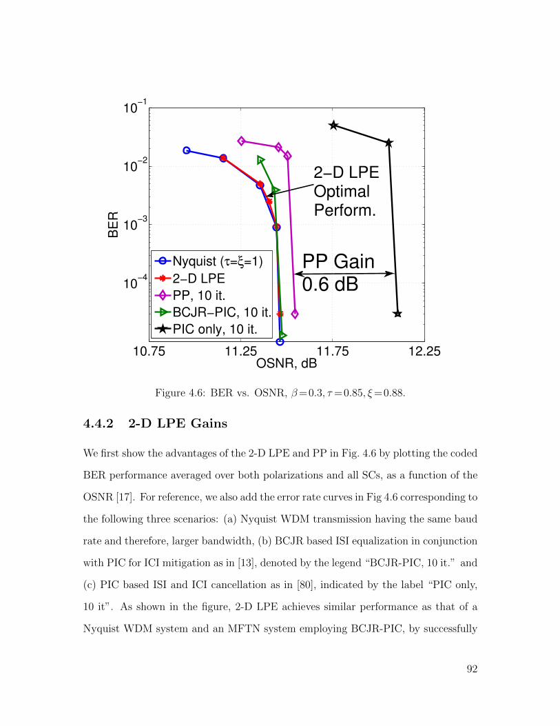
10.75 11.25 11.75 12.25

10−4

10−3

10−2

10−1

OSNR, dB

BE

R

Nyquist (τ=ξ=1)

2−D LPE

PP, 10 it.

BCJR−PIC, 10 it.

PIC only, 10 it.

PP Gain0.6 dB

2−D LPEOptimalPerform.

Figure 4.6: BER vs. OSNR, β=0.3, τ=0.85, ξ=0.88.

4.4.2 2-D LPE Gains

We first show the advantages of the 2-D LPE and PP in Fig. 4.6 by plotting the coded

BER performance averaged over both polarizations and all SCs, as a function of the

OSNR [17]. For reference, we also add the error rate curves in Fig 4.6 corresponding to

the following three scenarios: (a) Nyquist WDM transmission having the same baud

rate and therefore, larger bandwidth, (b) BCJR based ISI equalization in conjunction

with PIC for ICI mitigation as in [13], denoted by the legend “BCJR-PIC, 10 it.” and

(c) PIC based ISI and ICI cancellation as in [80], indicated by the label “PIC only,

10 it”. As shown in the figure, 2-D LPE achieves similar performance as that of a

Nyquist WDM system and an MFTN system employing BCJR-PIC, by successfully

92

0.7 0.75 0.8 0.85 0.9 0.95 10.5

0.6

0.7

0.8

0.9

1

τ

ξ

β = 0.1

β = 0.2

β = 0.3

β = 0.4

Feasible

(τ, ξ) Pairs

Figure 4.7: Feasible range of τ, ξ for 2-D LPE.

pre-equalizing the ISI and ICI completely. For this, 2-D LPE relies on simple non-

iterative filtering operations, as opposed to the substantially complex and buffer-space

constrained BCJR algorithm that is impractical especially for larger constellations.

Fig. 4.6 also suggests that PP yields 0.6 dB performance improvement over the PIC-

only receiver structure. Moreover, it produces sub-optimal performance compared to

the 2-D LPE for this particular combination of τ and ξ that is well within the range

specified by the inequality (4.5). However, as shown through the subsequent results,

PP is more effective for stricter values of τ and ξ pairs, for which 2-D LPE precoding

is infeasible.

93

10.8 11.7 12.6 13.5

10−4

10−3

10−2

10−1

OSNR, dB

BE

R

Nyquist (τ=ξ=1)

PP, 10 it.

BCJR−PIC, 10 it.

PIC only, 10 it.

PP Gain1.1 dB

Figure 4.8: BER vs. OSNR, β=0.3, τ=0.8, ξ=0.9.

4.4.3 Feasible Range for 2-D LPE

In Fig. 4.7, we plot the range of τ and ξ where the spectral factorization (4.2) and

thereby, 2-D LPE precoding is infeasible, for varying β. To numerically evaluate such

range of values that does not satisfy (4.6), we observe the presence of spectral zeros in

the overall TFP channel H(z). Fig. 4.7 indicates that higher values of the RRC roll-off

translates to a larger range of feasible τ and ξ values for the 2-D LPE. Furthermore,

we note that the plots in the figure also correspond to the inequality (4.5). This

means that the dimensionality and factorization constraints are equivalent for the

considered precoded TFP systems.

94

Table 4.1: Complexity, memory and latency, per codeword

Method Complexity Memory Latency

2-D LPE O(N2NfLw) O(NLb) O(Lb)

PP O((M+Lc+Nf)NImLw

)O(NLbIm) O(LbIm)

PIC-Only O((M+Lc+Ls)NImLw

)O(NLbIm) O(LbIm)

BCJR-PIC O((M

Ls2 +Lc)NImLw

)O(NLbIm) O(LbIm)

4.4.4 PP Gains

Finally, to show the usefulness of PP in more detail, we deliberately choose a pair of

time and frequency compression ratios in Fig. 4.8 such that (4.5) is violated for β=0.3,

and therefore, 2-D LPE can not be employed. Fig. 4.8 shows that the BCJR-PIC

outperforms PP by 0.65 dB at the price of significantly higher complexity. However,

under such transmission scenarios, PP offers 1.1 dB performance gains over PIC-only

equalization scheme having similar computational cost.

4.4.5 Computational Complexity

The details of the receiver complexity, latency and memory requirements for the dif-

ferent interference mitigation schemes are furnished in Table 4.1, where M , Ls, Lc,

Nf , Lb, Im denote the modulation order, truncated ISI and ICI-taps length, 1-D/2-

D LPE FFF taps length, LDPC codeword length in bits and the maximum turbo

iteration count, respectively, and Lw = Lb

log2Mis the number of modulated symbols

corresponding to each codeword. Values of the above parameters considered for our

simulations are mentioned at the beginning of this section. Benefits of the proposed

precoded systems can be seen in the performance-complexity trade-off, through suit-

able precoding technique selection depending on the MFTN parameters.

95

4.5 Conclusions

In this chapter, we presented two precoding approaches for the first time in MFTN

systems that enable packing of symbols in both time and frequency dimensions. First,

a matrix linear filtering based 2-D LPE precoding is proposed that performs joint

processing of the SCs to completely eliminate TFP ISI and ICI, and thereby, accom-

plishes optimal error rate performance. However, functionality of such precoding is

limited to a restricted range of time and frequency compression. Second, we presented

PP that facilitates independent processing of SCs at the transmitter for mitigating

ISI, but operates in an iterative fashion with the LDPC decoder, to eliminate ICI

at the receiver. Simulation results for a DP QPSK TFP WDM optical superchan-

nel suggests up to 1.1 dB performance gains by the proposed precoding techniques

over existing interference mitigation methods having similar or significantly higher

computational cost, buffer space and latency requirement.

96

Chapter 5

Towards Terabit-per-second

Super-Nyquist Systems

5.1 Introduction

Per-carrier data rates of 1 Tbps and more are being targeted in next generation

optical systems to cope with the increasing demands in network traffic[118]. TFP

superchannel transmission discussed in Chapter 4 is an attractive candidate to ac-

complish such a target. TFP offers SE improvements by allowing controlled overlap of

the SCs in time and frequency, and thereby introduces ISI and ICI. In Chapter 4, we

investigated precoded MFTN superchannel systems to pre-mitigate the TFP-ISI and

ICI. However, as shown in that chapter, the functionality of the presented precoding

methods was limited to a restricted range of time and frequency compression11, which

can enable only a benign packing of symbols. Therefore, they may be insufficient to

achieve the desired high SE targeted for the next generation Terabit systems [17].

Motivated by this, we consider spectrally more efficient TFP schemes that achieve

Tbps data rates. For this, we turn our focus to receiver-side high-performance ISIC

and ICIC schemes, as opposed to the transmitter-side precoding. By doing so, we

11While the PP presented in the previous chapter facilitates slightly larger range of frequencycompression compared to the 2-D LPE, PP is restrictive in terms of the amount of time-compressionachievable, depending on the value of the RRC roll-off. This is due to the fact that for each SC, PPemploys the 1-D LPE method presented in Chapter 2, which suffers from such restriction.

97

ensure that the TFP superchannel systems considered in this chapter are able to

facilitate a wider range of temporal and spectral overlap of the SCs.

Moreover, a superchannel signal may be subjected to additional narrow opti-

cal filtering due to multiple network elements, such as ROADMs implemented by

WSSs [118–120]. Such strict-filtering often leads to significant ISI for the edge-SCs of

a superchannel. Super-Nyquist transmission can be used to reduce such ISI by pack-

ing the SCs closer in both time and frequency, and thereby having a lower aggregate

signal BW.

In order to restrict the receiver-side complexity, at the beginning, we consider

frequency-packed (FP) transmissions, where the frequency-spacing of the optical car-

riers is reduced below the occupied BW of the individual SCs. We apply compu-

tationally simple linear equalization (LE)[18] and more powerful turbo PIC [81] to

mitigate the ICI. Thereafter, we study TFP transmission to further improve the

achievable SE [13]. To counter the additional ISI, Ungerboeck’s modified BCJR al-

gorithm [17] is employed for ISIC, in conjunction with the turbo-ICIC method. We

will show through our numerical results in Section 5.5 that with adequate signal pro-

cessing, super-Nyquist systems that are doubly constrained due to the filtering effects

of WSSs exhibit significant OSNR gains over Nyquist transmission, when targeting

Terabit data rates.

The contributions of this work are summarized as follows. For the first time,

a quantitative performance comparison of LE-ICIC and turbo-PIC based receiver

structures for coherent optical transmission is provided. While the application of

LE-ICIC for an optical system has been considered before, e.g. [18], PIC has only

been investigated in the TFP-literature under an AWGN channel assumption [13,

81]. Here, we apply turbo-PIC to high-baud-rate optical systems targeting 1 Tb/s

98

SC N

X-pol bitsLDPC Enc QAM

Map.RRC

Opt. Front-endY-pol bitsLDPC Enc QAM

Map.RRC

WD

M

...

...

SC 1

SC k

WSS ...

WSS

{m-ROADMs

Coh

. Rx

SSMF

Rx

DSP

D/AD/A

IQ

D/AD/A

IQ

A/DA/D

IQ

A/DA/D

IQ

RRC

RRC

Figure 5.1: Super-Nyquist WDM system model.

data rate in a 150 GHz BW considering practical fiber-optical impairments, and we

specify its performance gains over LE-ICIC. Second, we present an investigation of the

performance degradation due to narrow-filtering effects of cascaded ROADMs that are

integral components of the next-generation flexible-grid optical networks [119, 120].

In the context of a TFP transmission, consideration of such severe filtering effects on

the edge SCs of a superchannel is limited in the TFP-literature. In this chapter, to

achieve the target data rate under tight WSS filtering, we numerically quantify the

power-efficiency improvements due to TFP transmission over Nyquist WDM systems,

as opposed to the existing TFP works [17, 20, 21] that primarily focus on bandwidth-

efficiency evaluation, without considering aggressive WSS-filtering effects on the edge

SCs.

The remainder of the chapter is organized as follows. The system model is pre-

sented in Section 5.2. In Section 5.3, we conduct a performance comparison between

the LE-ICIC and the turbo-ICIC methods for the FP systems. We investigate the

BCJR-ISIC and the turbo-PIC approaches in Section 5.4. Section 5.5 presents the

simulation results. Finally, in Section 5.6 we provide concluding remarks.

99

5.2 System model

Figure 5.1 shows the block diagram of a DP super-Nyquist WDM superchannel trans-

mission. For each polarization branch, i.e. X and Y, of the kth SC, k∈ 1, 2, · · · , N ,

where N is the total number of SCs, an LDPC coded and modulated data stream ak

is pulse-shaped by an RRC filter h having a roll-off factor β. Following DAC conver-

sion, the electrical signal is converted to optical domain using individual lasers and

Mach-Zehnder (MZ) modulators to form the aggregate superchannel transmit signal.

The baseband equivalent analog signal for one polarization mode can be expressed

as

s(t) =∑l

∑k

ak[l]h(t− lτT )ej2π(k−N+12 )∆ft , (5.1)

where ∆f = ξ 1+βT

is the frequency-spacing between the adjacent SCs, with 0<τ ≤ 1

and ξ>0 denoting the time and frequency compression ratios, respectively, such that

τ = ξ= 1 corresponds to Nyquist signaling, 1τT

is the baud rate per SC, and l is the

symbol index. The transmitted WDM signal may be filtered by several WSSs while

propagating through the optical link. At the coherent receiver, the RRC matched-

filtered digital samples are fed as inputs to the Rx-DSP after conversion to electrical

domain by an integrated coherent receiver. For ease of characterization of the ISIC

and ICIC operations that use τT -sampled signals, we state the following lemma.

Lemma 5.1. Without optical impairments and noise, RRC matched filtered τT -

sampled signal for each polarization of the kth SC, k=1, 2, . . . , N , is given by

rk[n]=(ak[n] ? g0,0[n])+∑m6=k

(bk,m[n] ? g0,m−k[n]) , (5.2)

where ? denotes linear convolution, m= 1, 2, . . . , N , bk,m[n] = am[n]e−jω0(m−k)n, ω0 =

2π∆fτT , and gu,v denotes τT samples of fu(t) ? fv(t) with fu(t)=h(t)e−j2πu∆ft.

100

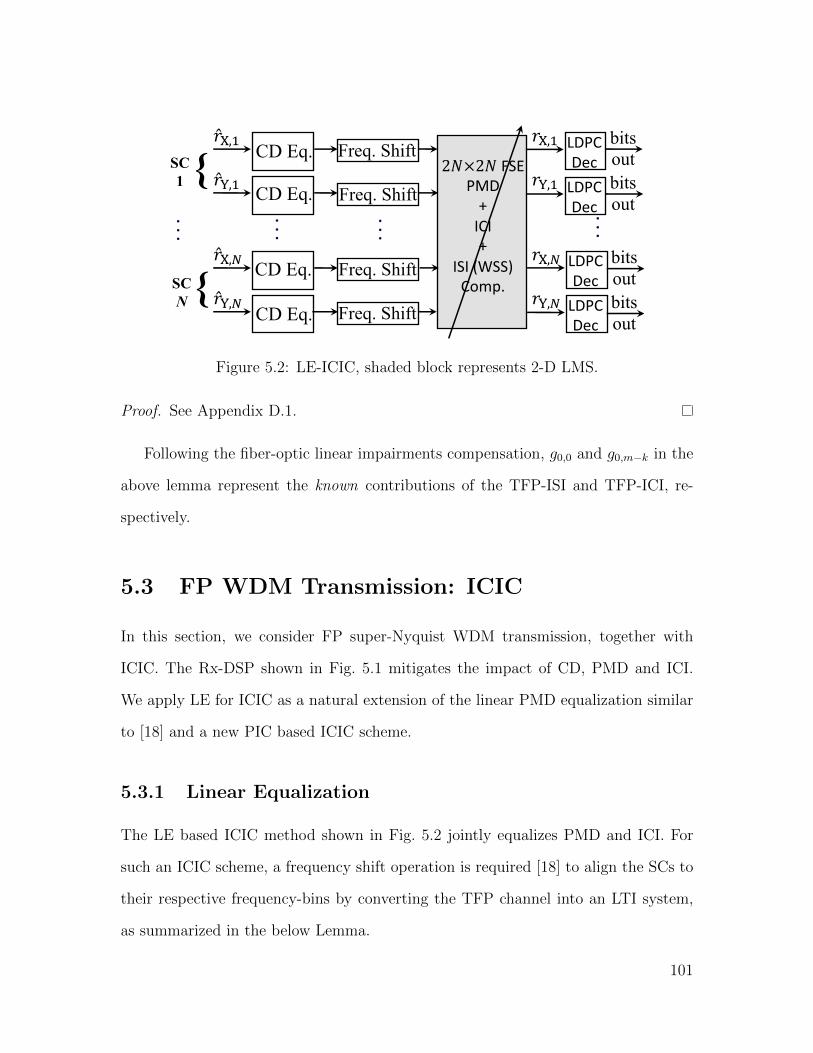
Freq. Shift"#,%

Freq. Shift"&,%

Freq. Shift"#,'

Freq. Shift"&,'

.........

2)×2) FSEPMD

+ICI+

ISI (WSS)Comp.

LDPC Dec

LDPC Dec

LDPC Dec

LDPC Dec

bits outbits out

bits outbits out

"#,%

"&,%

"#,'

"&,'

Linear ICI Cancellation

{SC 1

{SC N

...

CD Eq.

CD Eq.

CD Eq.

CD Eq.

Figure 5.2: LE-ICIC, shaded block represents 2-D LMS.

Proof. See Appendix D.1.

Following the fiber-optic linear impairments compensation, g0,0 and g0,m−k in the

above lemma represent the known contributions of the TFP-ISI and TFP-ICI, re-

spectively.

5.3 FP WDM Transmission: ICIC

In this section, we consider FP super-Nyquist WDM transmission, together with

ICIC. The Rx-DSP shown in Fig. 5.1 mitigates the impact of CD, PMD and ICI.

We apply LE for ICIC as a natural extension of the linear PMD equalization similar

to [18] and a new PIC based ICIC scheme.

5.3.1 Linear Equalization

The LE based ICIC method shown in Fig. 5.2 jointly equalizes PMD and ICI. For

such an ICIC scheme, a frequency shift operation is required [18] to align the SCs to

their respective frequency-bins by converting the TFP channel into an LTI system,

as summarized in the below Lemma.

101

CD Eq.��#,+,%

��&,+,%2×2 FSEPMD +

ISI (WSS)

... 𝑟#,+,%

𝑟&,+,%

+ Σ-

-LDPC DecLLR to

Soft SymICI Est.𝐼+,%,+

��#,+

��&,+2×2 FSEPMD +

ISI (WSS)

𝑟#,+

𝑟&,+

+ Σ-

-LDPC Dec

bits out 𝑖𝑡. = 𝑖𝑡.234

LLR789.𝑖𝑡. < 𝑖𝑡.234

LLR toSoft Sym

ICI Est.𝐼+,+,%ICI Est.𝐼+,+;%��#,+;%

��&,+;%2×2 FSEPMD +

ISI (WSS)

𝑟#,+;%

𝑟&,+;%

+ Σ-

LDPC DecLLR to

Soft Sym

ICI Est.𝐼+;%,+

...

-

... ...

Non-linear ICI Cancellation (SIC)

{SC k

{SC 𝑘 − 1

{SC 𝑘 + 1

CD Eq.

CD Eq.

CD Eq.

CD Eq.

CD Eq.

Figure 5.3: Turbo-PIC, shown for the X-pol. of the kth SC.

Lemma 5.2. The frequency shifts of the discrete time signal (5.2) for the kth SC, k=

1, 2, . . . , N , by an amount ω0

(k − N+1

2

)render the overall τT -sampled TFP channel

an LTI system, with respect to the rotated inputs ak[n]ejω0(k−N+12 ).

Proof. See Appendix D.2.

The CD compensated and frequency shifted received samples from both polar-

ization branches of all SCs are jointly processed by a 2N×2N 2-D adaptive LMS

based fractionally-spaced equalizer (FSE). The outputs of the joint equalizer are

soft-demapped and LDPC decoded to produce bits.

5.3.2 Iterative Equalization: Turbo-PIC

The proposed ICIC using iterative turbo-PIC for an optical superchannel is shown in

Fig. 5.3. Different from Fig. 5.2, the CD compensated received samples are processed

by a 2×2 adaptive LMS filter to mitigate the impact of PMD only. After polarization-

recovery is accomplished, turbo-PIC is subsequently employed for each polarization

102

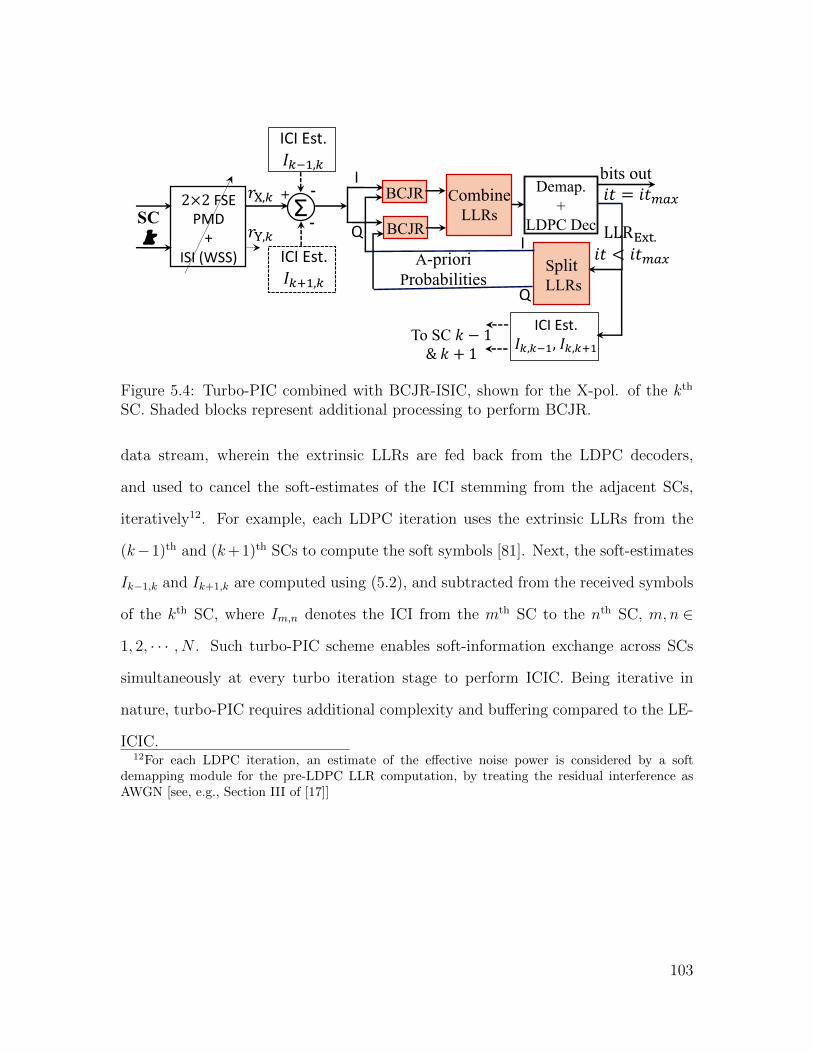
2×2 FSEPMD

+ISI (WSS)

𝑟#,+

𝑟&,+SC k

I

Q

BCJR

BCJR

CombineLLRs

Demap.+

LDPC Dec

SplitLLRs

LLR789.𝑖𝑡 < 𝑖𝑡234

I

Q

A-prioriProbabilities

+Σ

-

-

ICI Est.𝐼+,%,+

ICI Est.𝐼+;%,+

bits out 𝑖𝑡 = 𝑖𝑡234

ICI Est.𝐼+,+,%, 𝐼+,+;%

To SC 𝑘 − 1& 𝑘 + 1

Figure 5.4: Turbo-PIC combined with BCJR-ISIC, shown for the X-pol. of the kth

SC. Shaded blocks represent additional processing to perform BCJR.

data stream, wherein the extrinsic LLRs are fed back from the LDPC decoders,

and used to cancel the soft-estimates of the ICI stemming from the adjacent SCs,

iteratively12. For example, each LDPC iteration uses the extrinsic LLRs from the

(k−1)th and (k+1)th SCs to compute the soft symbols [81]. Next, the soft-estimates

Ik−1,k and Ik+1,k are computed using (5.2), and subtracted from the received symbols

of the kth SC, where Im,n denotes the ICI from the mth SC to the nth SC, m,n ∈

1, 2, · · · , N . Such turbo-PIC scheme enables soft-information exchange across SCs

simultaneously at every turbo iteration stage to perform ICIC. Being iterative in

nature, turbo-PIC requires additional complexity and buffering compared to the LE-

ICIC.12For each LDPC iteration, an estimate of the effective noise power is considered by a soft

demapping module for the pre-LDPC LLR computation, by treating the residual interference asAWGN [see, e.g., Section III of [17]]

103

5.4 TFP WDM Transmission: ISIC & ICIC

TFP WDM systems provide additional SE advantages over FP super-Nyquist systems

by transmitting the symbols at an FTN signaling rate [13]. Thereby, for a fixed baud

rate, FTN signaling translates to bandwidth compression of the individual SCs [17],

which reduces the amount of ISI introduced in the outer SCs in an FP superchannel

due to narrow WSS filtering. TFP transmission introduces ISI and ICI that are

perfectly known a-priori, and therefore, can be mitigated through static equalizers,

without the explicit need for channel estimation. To adjust the tap-coefficients of the

adaptive 2×2 PMD equalizer, the known TFP-induced interference is incorporated

in the desired signal generation [17] for the LMS algorithm. In this work, we employ

BCJR equalization based on Ungerboeck’s modeling [17] for TFP-ISIC. We consider

a truncated K-tap TFP-ISI channel, given by g0,0[n] in Lemma 5.1. Moreover, the

BCJR algorithm works in conjunction with turbo-PIC based ICIC as shown Fig. 5.4,

to facilitate an efficient TFP transmission. Exploiting the fact that TFP-ISI is real

valued, for a square-constellation, the I and Q components of the baseband received

samples are separately processed by the BCJR module to minimize computational

complexity. For each LDPC iteration, following the optical channel equalization,

and soft ICI cancellation via turbo-PIC, BCJR equalizes TFP-ISI by exchanging

extrinsic LLRs with the decoder, similar to [17]. At the final iteration, output bits

are generated from the LDPC decoders.

5.5 Results and Discussion

To show the effectiveness of the proposed TFP designs, we present a 400 Gbps and a

1 Tbps superchannel systems, employing QPSK and 16-QAM constellations, respec-

tively.

104

−100 −50 0 50 100−100

−80

−60

−40

−20

0

20

Frequency (GHz)

No

rma

lize

d P

SD

(d

B)

Before WSS

After WSS

WSS spectrum

ISIISI

3−dB

BW

No ICI

(a) ξ=1 (Nyq)

−100 −50 0 50 100−100

−80

−60

−40

−20

0

20

Frequency (GHz)

No

rma

lize

d P

SD

(d

B)

Before WSS

After WSS

WSS spectrum

less ISI less ISIICI

3−dB

BW

(b) ξ=0.7

Figure 5.5: 400 Gbps system, normalized PSD vs. frequency, with 4 WSSs.

−100 −50 0 50 100−80

−60

−40

−20

0

20

Frequency (GHz)

Norm

aliz

ed P

SD

(dB

)

Before WSS

After WSS

WSS spectrum

ISI No ICI ISI

3−dB

BW

(a) ξ=1 (Nyq)

−100 −50 0 50 100−80

−60

−40

−20

0

20

Frequency (GHz)

Norm

aliz

ed P

SD

(dB

)

Before WSS

After WSS

WSS spectrum

3−dB

BW

less ISI less ISIICI

(b) ξ=0.8

Figure 5.6: 1 Tbps system, normalized PSD vs. frequency, with 4 WSSs.


We consider a dual-carrier DP QPSK 400 Gbps system in a 100 GHz BW with per

SC baud rate of 62.5 Gbaud, and a 1 Tbps DP 16-QAM system that uses 3 SCs

packed within 150 GHz with a baud rate of 52.09 Gbaud per SC. For the simula-

tions, a 1040 km SSMF with CD parameter value −21 ps2/km and PMD parameter

105

15 20 2510

−6

10−5

10−4

10−3

10−2

10−1

OSNR, dB

BE

R

No

WSS

1WSS

4WSS

No WSS

Nyq

ξ = 0.95

ξ = 0.9

ξ = 0.85

ξ = 0.8

ξ = 0.7

ξ = 0.5

(a) LE ICIC

15 20 2510

−6

10−5

10−4

10−3

10−2

10−1

OSNR, dB

BE

R

No

WSS

4WSS

1WSS

No WSS

Nyq

ξ = 0.95

ξ = 0.9

ξ = 0.85

ξ = 0.8

ξ = 0.7

ξ = 0.5

(b) Turbo-PIC

Figure 5.7: 400 Gbps system, BER vs OSNR for FP WDM systems.

0.5 ps/√

km, RRC roll-off β = 0.1, and LDPC codes with rate 0.8 and codeword-

length 64800 bits are adopted, with varying τ and ξ. Each WSS is modeled as a

6th-order Gaussian filter, whereby 1 and 4 WSS stages correspond to effective 3-dB

BWs of 100 GHz and 89.3 GHz for the 400 Gbps system, and 150 GHz and 133.7 GHz

for the 1 Tbps system, respectively. We use 33 T2-spaced taps for the LE-ICIC, and a

maximum iteration count of 10 for the turbo-PIC. Perfect frequency synchronization

and phase-lock is assumed for the simulations. Considering 13 spans of SSMFs with

an attenuation constant of 0.2 dB/km and span length of 80 km, the launch power

is set as −5 dBm per SC, for which nonlinear distortions are not significant [20].

5.5.2 ISI vs. ICI Trade-off

First, we consider FP super-Nyquist systems. The normalized PSDs of the 400 Gbps

system and the 1 Tbps WDM system, filtered through 4 WSSs, are shown in Fig. 5.5a-

5.5b and Fig. 5.6a-5.6b, respectively, for the Nyquist and FP configurations. As

shown in Fig. 5.5a and Fig. 5.6a, the SCs located at the edges in a Nyquist WDM

106

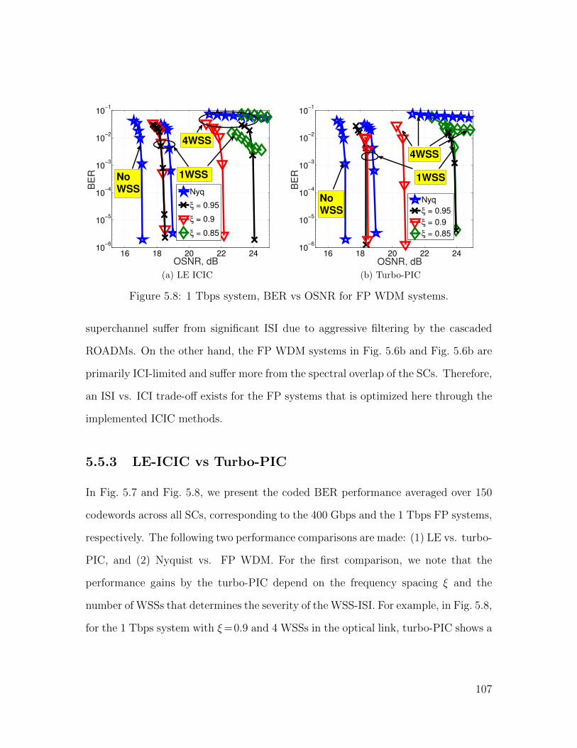
16 18 20 22 2410

−6

10−5

10−4

10−3

10−2

10−1

OSNR, dB

BE

R

1WSS

4WSS

No

WSS Nyq

ξ = 0.95

ξ = 0.9

ξ = 0.85

(a) LE ICIC

16 18 20 22 2410

−6

10−5

10−4

10−3

10−2

10−1

OSNR, dB

BE

R

No

WSS

1WSS

4WSS

Nyq

ξ = 0.95

ξ = 0.9

ξ = 0.85

(b) Turbo-PIC

Figure 5.8: 1 Tbps system, BER vs OSNR for FP WDM systems.

superchannel suffer from significant ISI due to aggressive filtering by the cascaded

ROADMs. On the other hand, the FP WDM systems in Fig. 5.6b and Fig. 5.6b are

primarily ICI-limited and suffer more from the spectral overlap of the SCs. Therefore,

an ISI vs. ICI trade-off exists for the FP systems that is optimized here through the

implemented ICIC methods.

5.5.3 LE-ICIC vs Turbo-PIC

In Fig. 5.7 and Fig. 5.8, we present the coded BER performance averaged over 150

codewords across all SCs, corresponding to the 400 Gbps and the 1 Tbps FP systems,

respectively. The following two performance comparisons are made: (1) LE vs. turbo-

PIC, and (2) Nyquist vs. FP WDM. For the first comparison, we note that the

performance gains by the turbo-PIC depend on the frequency spacing ξ and the

number of WSSs that determines the severity of the WSS-ISI. For example, in Fig. 5.8,

for the 1 Tbps system with ξ=0.9 and 4 WSSs in the optical link, turbo-PIC shows a

107

1.4 dB required OSNR (ROSNR)13 gain over the LE-ICIC. For the 400 Gbps system

with the same configuration, this gain is observed to be 1.7 dB in Fig. 5.7. Moreover,

we observe that for FP super-Nyquist systems, an optimal value of ξ exists. This is

highlighted in Fig. 5.9 and Fig. 5.10 for the case of 4 WSSs, corresponding to the

400 Gbps and the 1 Tbps systems, respectively, where ROSNR is plotted as a function

of ξ. Comparing the results for the FP super-Nyquist and the Nyquist WDM systems

in Fig. 5.8, we observe moderate gains of 0.6 dB dB for the case of 1 WSS for the

1 Tbps transmission. However, with 4 WSSs in the optical link, the FP super-Nyquist

system having ξ = 0.9 yields substantial performance gain over the Nyquist WDM

system that exhibits a high BER-floor due to severe WSS-ISI, as shown in Fig. 5.8.

For the 400 Gbps system in Fig. 5.7b, an FP gain of 2.95 dB over Nyquist signaling

is observed when turbo-ICIC is employed with ξ = 0.9. Further reduction of ξ to

reduce the impact of WSS-ISI induces additional FP-ICI that even the turbo-PIC is

unable to address.

5.5.4 TFP Gains

Additional ROSNR advantages over Nyquist signaling can be obtained by super-

Nyquist WDM systems that enable TFP transmission. We illustrate such gains by

means of error rate plots in Fig. 5.11 and Fig. 5.12 for the 400 Gbps and the 1 Tbps

WDM systems, respectively, with 4 WSSs in the optical link. For the ISIC, we use

truncated TFP-ISI channel such that K=3 and 4 for the 1 Tbps system correspond

to 64 and 256-state BCJR, respectively. Similarly, for the 400 Gbps transmission, we

use K=3 and 6, and thereby, employing 8 and 64-state BCJR modules, respectively.

Our goal is to optimize the average BER performance over different (τ, ξ) pairs. For

13We measure the ROSNR in the post-waterfall region of the BER curves with BER < 10−5, sothat practically error-free transmission is achieved.

108

17.3

18.3

19.3

20.3

0.7 0.75 0.8 0.85 0.9 0.95 1

RO

SNR

[d

B]

ξ

Linear ICICTurbo-PIC

𝝃𝐨𝐩𝐭

Figure 5.9: 400 Gbps, ROSNR vs. ξ, with 4 WSSs, illustrating the optimal ξ.

20.5

22.5

24.5

0.875 0.9 0.925 0.95 0.975

ROSN

R [d

B]

ξ

Linear ICICTurbo-PIC

𝝃𝐨𝐩𝐭

1.4 dB

Figure 5.10: 1 Tbps, ROSNR vs. ξ, with 4 WSSs, illustrating the optimal ξ.

performance comparison, we also include the BER plots of the FP super-Nyquist

systems corresponding to the optimal ξ derived through Fig. 5.7-5.10. Additionally,

we include the performance of the Nyquist WDM systems without WSS and with

109

10 15 20 25 3010

−6

10−5

10−4

10−3

10−2

10−1

OSNR, dB

BE

R

6.6dB

7.7dB

3.65 dB

(τ, ξ) pairs

4WSS

NoWSS

Opt. FPNyq, τ = ξ = 1

(1,0.9)

(0.85,0.8),3taps

(0.9,1),3taps

(0.8,1),3taps

(0.8,0.9),3taps

(0.8,0.9),6taps

Figure 5.11: 400 Gbps, BER vs. OSNR, with 4 WSSs, illustrating additional TFPgains.

4 WSSs, as a reference. As shown in Fig. 5.12 for the 1 Tbps system, an optimal

τ and ξ combination using BCJR-ISIC with K = 3 significantly outperforms the

Nyquist-WDM transmission that shows high BER floor. Furthermore, such TFP

transmission yields 0.4 dB ROSNR improvement over the optimized FP system that

employs optimal frequency-spacing. An additional performance gain of 0.7 dB for

the 1 Tbps transmission, corresponding to K = 4, is achieved by the same TFP

transmission at the price of increased BCJR complexity. Similar patterns are also

observed for the 400 Gbps system in Fig. 5.11, where as high as 7.7 dB ROSNR

gain is achieved by the optimized TFP transmission over the Nyquist WDM system

having the same data rate.

110

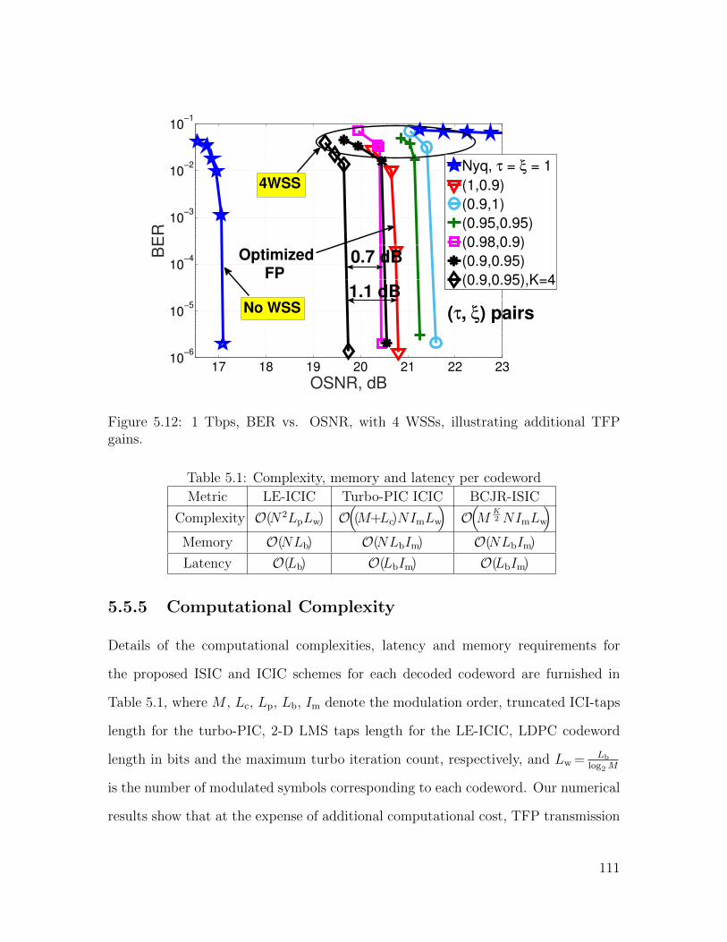
17 18 19 20 21 22 2310

−6

10−5

10−4

10−3

10−2

10−1

OSNR, dB

BE

R

Optimized FP

0.7 dB

1.1 dB

(τ, ξ) pairs

4WSS

No WSS

Nyq, τ = ξ = 1

(1,0.9)

(0.9,1)

(0.95,0.95)

(0.98,0.9)

(0.9,0.95)

(0.9,0.95),K=4

Figure 5.12: 1 Tbps, BER vs. OSNR, with 4 WSSs, illustrating additional TFPgains.

Table 5.1: Complexity, memory and latency per codeword

Metric LE-ICIC Turbo-PIC ICIC BCJR-ISIC

Complexity O(N2LpLw) O((M+Lc)NImLw

)O(M

K2 NImLw

)Memory O(NLb) O(NLbIm) O(NLbIm)

Latency O(Lb) O(LbIm) O(LbIm)

5.5.5 Computational Complexity

Details of the computational complexities, latency and memory requirements for

the proposed ISIC and ICIC schemes for each decoded codeword are furnished in

Table 5.1, where M , Lc, Lp, Lb, Im denote the modulation order, truncated ICI-taps

length for the turbo-PIC, 2-D LMS taps length for the LE-ICIC, LDPC codeword

length in bits and the maximum turbo iteration count, respectively, and Lw = Lb

log2M

is the number of modulated symbols corresponding to each codeword. Our numerical

results show that at the expense of additional computational cost, TFP transmission

111

with efficient interference mitigation techniques can significantly improve the super-

Nyquist performance in the presence of narrow WSS-filtering, by optimizing the time

and frequency spacing parameters. Our numerical results also suggest that such

improvements are not achievable by packing the WDM carriers in either time or

frequency dimension alone.

5.6 Conclusions

In this chapter, we developed designs for high data rate TFP superchannel trans-

missions that may be subject to aggressive filtering due to WSS. At the expense

of introducing deliberate known interference, super-Nyquist systems can effectively

reduce the impact of such narrow-filtering by packing the SCs more efficiently. This

requires powerful ICI mitigation schemes such as the presented turbo-PIC. Simulation

results show that by employing BCJR based ISIC, together with LE or turbo ICIC,

super-Nyquist WDM systems targeting 400 Gbps data rate in a 100 GHz BW, and

1 Tbps data rate in a 150 GHz channel, offer significant ROSNR gains over Nyquist

transmission under similar conditions.

112

Chapter 6

Flexible Designs for Spectrally

Efficient Time Frequency Packed

Superchannels

6.1 Introduction

We have seen in the previous chapter that TFP WDM superchannel transmission is

an attractive, spectrally efficient technology to achieve Terabit data rates in long-

haul OFC systems. In the existing optical super-Nyquist literature, time-only [14,

17, 78, 79] and frequency-only [16, 18–20] packing have been considered quite exten-

sively, which introduce either ISI or ICI. However, packing the symbols in both time

and frequency dimensions can theoretically provide higher achievable rates [13], at

the price of introducing ISI and ICI simultaneously. For the TFP designs proposed

in Chapter 5, the employed powerful ISIC and ICIC algorithms exploited the known

information about the TFP ISI and ICI channel, without performing additional chan-

nel estimation operation. However, as we will show in this chapter, an interference

channel estimation approach can offer significant performance improvement for the

considered TFP transmission targeting Tbps data rates.

Another practical challenge that affects WDM transmission is the signal distortion

113

caused by PN stemming from the spectral linewidth of the transmitter and receiver

laser beams [83, 84]. However, the TFP receiver designs in Chapter 4 assumed perfect

CPR, and therefore, no PN compensation algorithm was presented for the considered

TFP systems. It is important to note that the application of HoM formats makes the

communication systems more sensitive to PN. Moreover, the impact of PN is more

severe for TFP superchannels, since the presence of ISI and ICI precludes the direct

application of off-the-shelf PN mitigation algorithms that are tailored to Nyquist

transmission [70, 82, 84]. Therefore, we need sophisticated signal processing tools to

counter TFP interference together with powerful PN cancellation strategies.

In this chapter, we consider both temporal and spectral overlap of the SCs to

enable a flexible TFP superchannel transmission. To accomplish this, we present

signal processing techniques to efficiently mitigate TFP interference, fiber-optical

non-idealities, and PN. This work encompasses the following three novel contribu-

tions.

1. A joint ISI and ICI channel estimation method, coupled with PMD equaliza-

tion and a coarse PN estimation (CPNE) is proposed. While the TFP-induced

interference channel is a-priori known [121], such estimation is necessary be-

cause (a) estimating the exact number of ISI taps required by the BCJR-ISIC

and forcing the remaining ISI-taps to zero can lead to significant performance

improvement [17], and (b) interference stemming from additional sources in the

optical link, such as the electrical/optical filters, can be accounted for. In con-

junction with PMD equalization and interference channel estimation, we also

jointly perform a coarse CPR, which is beneficial since (a) it facilitates better

TFP channel estimation by minimizing the overall MSE during the initial pilots

transmission phase, and (b) it offers improved bootstrapping for more sophis-

114

ticated iterative PN mitigation schemes to clean up the residual PN, especially

when LLW is high, and HoM formats are used.

2. A novel, iterative, modulation-format-independent PN estimation method, in

the form of post-FEC refined adaptation, is proposed. Moreover, the FG-

based solutions presented in [17] and [70] are also properly amended to account

for the TFP ISI and ICI. While the authors of [17] consider post-FEC hard

decisions for the FG metric computations for the case of only TFP-ISI and

QPSK transmission, we use soft information to improve robustness against

error-propagation in HoM systems in the presence of both ISI and ICI.

3. A serial-and-parallel combined interference cancellation (SPCIC) based ICIC

scheme is presented. Different from the existing PIC structures [13, 80, 117],

the proposed SPCIC encapsulates a conceptual combination of the SIC and

the PIC paradigms, to offer performance improvements. The proposed ICIC

solution in tandem with BCJR-ISIC is shown to exhibit excellent tolerance to

high LLW and aggressive optical filtering due to cascaded ROADM nodes that

may be present in the fiber link.

The remainder of the chapter is organized as follows. The system model is intro-

duced in Section 6.2. In Section 6.3, we propose a joint TFP-interference and a CPNE

strategy. In Section 6.4, we investigate two iterative CPR algorithms. Proposed TFP

interference mitigation techniques are detailed in Section 6.5, followed by numerical

results for optical TFP systems presented in Section 6.6. Finally, Section 6.7 provides

concluding remarks.

115

SC N

X-pol bitsLDPC Enc QAM

Map.RRC

Opt. Front-endY-pol bits

LDPC Enc QAMMap.

RRC

WD

M

...

...

SC 1

SC k

Coh

. Rx

SSMF

DSP

D/AD/A

IQ

D/AD/A

IQ

A/DA/D

IQ

A/DA/D

IQ

RRC

RRC

Figure 6.1: TFP WDM system model.

6.2 System Model

In this work, we consider a DP TFP WDM transmission for longhaul optical fiber

communication [14, 17]. The schematics of such a system are shown in Fig. 6.1. For

each of the X and Y polarization data streams of the mth SC, m∈1, 2, · · · , N , with

N being the total number of SCs, an LDPC coded and modulated data stream xm

is shaped by an RRC pulse p with a roll-off factor β. The digital samples are then

transformed into analog signals via digital-to-analog converters (DACs), followed by

conversion to the optical domain using individual lasers and MZ modulators. The

equivalent baseband transmitted signal for the X-polarization branch can be written

as

sx(t)=∑l

∑m

xm[l]p(t−lτT )ej(

2π(m−N+12 )∆ft+θ

(m)tx (t)

), (6.1)

where ∆f=ξ 1+βT

is the frequency-spacing between the adjacent SCs, τ and ξ are the

time and frequency compression ratios, respectively, such that τ = ξ= 1 corresponds

to the Nyquist WDM system, l is the symbol index, 1τT

is the per-SC baud rate, and

θ(m)tx is the transmitter laser PN corresponding to the mth SC.

The transmitted superchannel signal propagates through multiple spans of SSMFs,

whereby the optical signal suffers distortion due to fiber-optical impairments, such as

the CD and the PMD [60, 96, 122]. In the presence of CD and the first-order PMD,

116

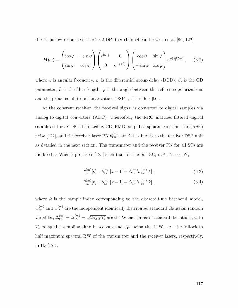
the frequency response of the 2×2 DP fiber channel can be written as [96, 122]

H(ω) =

cosϕ − sinϕ

sinϕ cosϕ

ejω

τd2 0

0 e−jωτd2

cosϕ sinϕ

− sinϕ cosϕ

e−jβ22Lω2

, (6.2)

where ω is angular frequency, τd is the differential group delay (DGD), β2 is the CD

parameter, L is the fiber length, ϕ is the angle between the reference polarizations

and the principal states of polarization (PSP) of the fiber [96].

At the coherent receiver, the received signal is converted to digital samples via

analog-to-digital converters (ADC). Thereafter, the RRC matched-filtered digital

samples of the mth SC, distorted by CD, PMD, amplified spontaneous emission (ASE)

noise [122], and the receiver laser PN θ(m)r,x , are fed as inputs to the receiver DSP unit

as detailed in the next section. The transmitter and the receiver PN for all SCs are

modeled as Wiener processes [123] such that for the mth SC, m∈1, 2, · · · , N ,

θ(m)tx [k]= θ

(m)tx [k − 1] + ∆

(m)tx w

(m)tx [k] , (6.3)

θ(m)rx [k]= θ(m)

rx [k − 1] + ∆(m)rx w(m)

rx [k] , (6.4)

where k is the sample-index corresponding to the discrete-time baseband model,

w(m)tx and w

(m)rx are the independent identically distributed standard Gaussian random

variables, ∆(m)tx = ∆

(m)rx =

√2πfWTs are the Wiener process standard deviations, with

Ts being the sampling time in seconds and fW being the LLW, i.e., the full-width

half maximum spectral BW of the transmitter and the receiver lasers, respectively,

in Hz [123].

117

CD Eq.

mth SC

CD Eq.X-polY-pol

2x2PMD Eq

Coh.Rx

ISIICI

CPNEPMD filt.

CD Eq. outputsfrom other SCs

Known pilots

{LMS-basedEstimates

XX

de-rotation

Feedforward loop Feedback loop

SIC/PIC

BCJRBCJRBCJRBCJR

LDPC Dec

LDPC Dec

LMS/FGIPNE

Post-FEC LLRs/Hard-decisionsfrom other SCs

de-rotationde-rotationde-rotation

Post-FEC LLRs

Bits out

: Blocks After LDPC iterations: Scalar signals: Vector signals

Post-FEC LLRs: Estimation modules

X-polY-pol

Post-FEC LLRs from other SCS

Figure 6.2: Jointly estimating PMD filter, TFP interference and PN.

6.3 Interference Channel Estimation and CPNE

Inspired by the algorithm presented in [17], we propose an adaptive TFP receiver de-

sign, where we jointly estimate the TFP-interference channel, the 2×2 PMD equalizer

tap co-efficients, and perform a coarse estimation of the laser PN. Different from [17],

that restricts itself to ISI channel estimation only, in this work, we estimate the ISI

and the ICI impulse responses simultaneously, coupled with a coarse CPR. More-

over, we also enforce the real-valued constraint on the ISI-taps adaptation algorithm

to employ a reduced-complexity BCJR equalization by separately processing the I

and Q components. We will show through the numerical results in Section 6.6 that

such an adaptive strategy facilitates flexible superchannel transmission by offering

significant performance advantages over non-adaptive TFP design, such as the one

presented in Chapter 5.

118

6.3.1 DSP Modules

The receiver DSP design is shown in Fig. 6.2 for the mth SC of the TFP superchannel.

As shown in the figure, the received signal in each polarization branch is first processed

by a time-invariant CD compensating filter implemented in the frequency domain

through overlap-and-add method [60, 96, 122]. Thereafter, the CD equalized samples

are filtered by a fractionally-spaced 2 × 2 PMD equalizer to remove the cross-talk

between the two polarization streams. The estimates of the PMD filter coefficients,

TFP-interference channel and a coarse PN are obtained through a pilot symbols-

aided LMS-based adaptation algorithm, the details of which are relegated to the

next subsection. Following the polarization recovery, PN cancellation per polarization

branch for each SC is accomplished by using the CPNEs or the iterative PN estimates.

Next, the PN corrected received signal is processed by the turbo ICIC and the BCJR-

ISIC modules. After decoding, soft informations in the form of LLRs are fed back from

the LDPC decoders to mitigate TFP interference and PN, iteratively. The details of

the iterative PN cancellation structure, together with ICIC and ISIC operations will

be presented in Sections 6.4 and 6.5.

6.3.2 LMS Update Equations

To derive the update equations for the joint estimation algorithm, we formulate the

column vectors a(m)k and u

(m)k corresponding to the constellation symbols and the

input samples to the 2×2 PMD equalizer, respectively, by stacking the X and Y

polarized signals of the mth SC at the kth sample time. The error signal is then

computed as the difference between the phase-rotated PMD filter output and the

“desired signal” [17], whereby the desired signal computation incorporates the effects

of the TFP interference into the clean pilot symbols, as shown below. The combined

119

error signal vector with the X and Y polarization symbols is written as

ε(m)k = [ε

(m)k,x, ε

(m)k,y]T = z

(m)k︸︷︷︸

filtered output

� [e−jθ(m)x,k , e−jθ

(m)y,k ]T︸︷︷︸

phase rotation

− d(m)k︸︷︷︸

desired signal

, (6.5)

where

z(m)k = [z

(m)x,k , z

(m)y,k ]T =

Nw−1∑i=0

W(m)i,k u

(m)k−i , (6.6)

d(m)k = [δ

(m)k,x, δ

(m)k,y]T =

Ls∑j=−Ls

h(m)j,k � a

(m)k−j +

∑n 6=m

Lc∑ν=−Lc

g(n,m)ν,k � a

(n)k−ν . (6.7)

In (6.5)-(6.7), ε(m)k,x/y, z

(m)k,x/y and δ

(m)k,x/y are respectively the error signal, PMD filtered

output and the desired signal corresponding to the X or the Y polarization (the

subscript x/y means “X respectively Y”) for the mth SC at the kth sample time,

W(m)i,k is the ith matrix-tap of the T

2-spaced PMD equalizer, Nw is the total number

of PMD filter taps, h(m)j,k and g

(n,m)ν,k are the jth and the νth symbol-spaced ISI and

ICI tap vector, respectively, with Ls and Lc being the total number of ISI and ICI

channel taps, respectively, [· · · ]T denotes the transpose of a vector, � denotes the

elementwise vector product, and a(n)k =a

(n)k e±j2π∆fk denotes the rotated constellation

symbol for the nth SC, with ± sign determined from (6.1) depending on the relative

positions of the SCs.

From (6.5), we define the MSE as

Mtot = E

(N∑m=1

‖ε(m)k ‖

2

), (6.8)

where E(·) denotes the expectation operator. For ease of formulation of the LMS

120

update equations based on the gradient decent algorithm [104], we exploit the sym-

metry of the TFP channel by enforcing the real and symmetry condition on the ISI

impulse response, and conjugate symmetry on the ICI channel, such that

h(m)j,k =

(h

(m)j,k

)∗, m∈ {1, 2, . . . , N},−Ls≤j≤Ls ,

h(m)j,k = h

(m)−j,k , m∈ {1, 2, . . . , N},−Ls≤j≤Ls ,

g(n,m)ν,k =

(g

(n,m)−ν,k

)∗, n∈ {1, 2, . . . , N},−Lc≤ν≤Lc.

Finally, computing the gradients ∂Mtot

∂W(m)α,k

, ∂Mtot

∂h(m)β,k

, ∂Mtot

∂g(m)γ,k

and ∂Mtot

∂θ(m)x/y,k

, where 0 ≤ α ≤

Nw − 1, 0 ≤ β ≤ Ls, 0 ≤ γ ≤ Lc, we can write the LMS update equations as

W(m)α,k+1 =W

(m)α,k − µw

([ejθ

(m)x,k , ejθ

(m)y,k ]T� ε(m)

k

)(u

(m)k−α

)H

, (6.9)

h(m)β,k+1 =h

(m)β,k + µhRe

[(ε

(m)k �

(a

(m)k−β+a

(m)k+β

)∗)], (6.10)

g(n,m)γ,k+1 =g

(n,m)γ,k + µg

(ε

(n)k �

(a

(m)k−γ

)∗+(ε

(n)k

)∗� a(m)

k+γ

), (6.11)

θ(m)x/y,k+1 = θ

(m)x/y,k + µθIm

[ (δ

(m)x/y,k

)∗z

(m)x/y,ke

−jθ(m)x/y,k

]. (6.12)

where µw>0, µh>0 and µg>0 are the step size parameters, Re[·], (·)∗ and (·)H denote

the real-part, complex conjugation and matrix Hermitian operations, respectively.

6.3.3 Data-aided and Decisions-directed Adaptation

To initiate the above adaptive estimation algorithm and accomplish LMS conver-

gence, we exploit the continuous pilot symbols transmission during the link-setup

phase at the beginning of data transmission [17, 20, 78]. Thereafter, the CPNEs

and PMD filter taps are slowly adjusted based on the blocks of Np periodic pilot

symbols inserted uniformly across the data frame after every Nd data symbols, to

121

continuously track PN and the slow rotation of the PSP [60, 96, 122, 124]. The

pilot symbols density p= Np

Np+Ndis chosen to meet a desired trade-off between per-

formance and transmission overhead. From the CPNEs obtained during the periodic

pilots transmission, interpolation strategies are adopted to account for PN variation

over each symbol duration. In this chapter, we apply linear interpolation for such

purposes. To remove the residual PN, the CPNEs thus obtained in every symbol

duration are used to bootstrap more powerful FG-based and LMS-based iterative

PN mitigation algorithms presented in the next section. Since the TFP interference

channel is not likely to change over the course of the transmission, the ISI and ICI

impulse responses can be estimated only once during the link-setup, followed by very

slow adjustments based on the post-LDPC symbol-decisions [17].

6.4 Iterative PN Estimation (IPNE)

After the LMS-based coarse CPR is accomplished, we employ more involved iterative

algorithms to remove the residual PN. At each LDPC iteration, the a-posteriori LLRs

are fed back from the decoders for the purposes of (a) iterative PN estimation and

compensation, and (b) TFP interference cancellation as detailed in Section 6.5. In

this section, we present two IPNE schemes, namely the low-complexity LMS-based

IPNE (LIPNE) and the high-performance factor graph based IPNE (FGIPNE) [70].

The LIPNE, which requires low computational cost and buffer-space, offers decent

performance for small values of LLW. Additionally, the functionality of the LIPNE

does not depend on the modulation format and the explicit knowledge of the PN

statistics. On the other hand, the FGIPNE shows excellent tolerance to strong PN

and severe TFP interference, at the expense of modulation format dependency, higher

complexity, and buffering. Moreover, the computation of the FGIPNE metrics re-

122

quires an estimate of the aggregate variance of the combined Wiener processes of the

transmitter and receiver laser PN [70]. Depending on the specific TFP application

scenario, the most suitable IPNE method can be chosen such that a desired trade-off

between performance and complexity is achieved. An analysis of such trade-off is

investigated in Section 6.6.

6.4.1 LIPNE

For this scheme, we refine the LMS based CPNEs obtained in (6.12) for each symbol

duration, using the LLRs fed back from the LDPC decoders to make hard symbol-

decisions. To account for the TFP ISI and ICI, we design the effective pilots by

reconstructing the desired signals δ(m)x/y,k according to (6.7) at every iteration, using

the estimated TFP interference channel and the hard-decisions of symbols from all

SCs.

While such post-LDPC decision-directed LIPNE is computationally simpler than

other state-space based iterative methods, it may produce sub-optimal performance

due to the error-propagation when hard-symbol decisions are erroneous, especially

with HoM in the presence of severe ISI and ICI. As shown through the numerical

results in Section 6.6, LPINE for TFP systems incur performance degradation when

LLW is high. Motivated by this, we investigate the more powerful FGIPNE approach

presented in [70], whereby we slightly modify the metric computation to account for

the TFP-ISI and ICI.

6.4.2 FGIPNE

We take into account the TFP interference by amending the state-space based FGIPNE

algorithm in [70] to tailor it to our considered super-Nyquist transmission. We re-

123

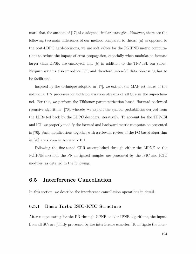
mark that the authors of [17] also adopted similar strategies. However, there are the

following two main differences of our method compared to theirs: (a) as opposed to

the post-LDPC hard-decisions, we use soft values for the FGIPNE metric computa-

tions to reduce the impact of error-propagation, especially when modulation formats

larger than QPSK are employed, and (b) in addition to the TFP-ISI, our super-

Nyquist systems also introduce ICI, and therefore, inter-SC data processing has to

be facilitated.

Inspired by the technique adopted in [17], we extract the MAP estimates of the

individual PN processes for both polarization streams of all SCs in the superchan-

nel. For this, we perform the Tikhonov-parameterization based “forward-backward

recursive algorithm” [70], whereby we exploit the symbol probabilities derived from

the LLRs fed back by the LDPC decoders, iteratively. To account for the TFP-ISI

and ICI, we properly modify the forward and backward metric computation presented

in [70]. Such modifications together with a relevant review of the FG based algorithm

in [70] are shown in Appendix E.1.

Following the fine-tuned CPR accomplished through either the LIPNE or the

FGIPNE method, the PN mitigated samples are processed by the ISIC and ICIC

modules, as detailed in the following.

6.5 Interference Cancellation

In this section, we describe the interference cancellation operations in detail.

6.5.1 Basic Turbo ISIC-ICIC Structure

After compensating for the PN through CPNE and/or IPNE algorithms, the inputs

from all SCs are jointly processed by the interference canceler. To mitigate the inter-

124

ICI gen𝐼",$

𝑟&,$ +Σ-

-LDPCDec

bits out 𝐢𝐭 = 𝐢𝐭𝐦𝐚𝐱

𝐋𝐋𝐑𝟏 ≤ 𝐢𝐭 < 𝐢𝐭𝒎𝒂𝒙

LLR toSoft Sym

ICI gen𝐼$,"

ICI gen𝐼$,5

ICI gen𝐼5,$

SC 2X-pol. BCJR

𝟏 ≤ 𝐢𝐭 < 𝐢𝐭𝒎𝒂𝒙

𝟏 ≤ 𝐢𝐭 < 𝐢𝐭𝒎𝒂𝒙

To SC 1

To SC 3

𝐢𝐭𝟏 < 𝐢𝐭 < 𝐢𝐭𝒎𝒂𝒙

𝐢𝐭𝟏 < 𝐢𝐭 < 𝐢𝐭𝒎𝒂𝒙

From SC 1

From SC 3

𝑟&,$6789:

Figure 6.3: BCJR-ISIC+SPCIC-ICIC, shown for the example of a 3-SC WDM sys-tem.

ference induced by the TFP transmission, the ISI and ICI impulse responses estimated

in Section 6.3 are provided as inputs to the ISIC and ICIC modules, respectively. For

ISIC, the BCJR algorithm based on Ungerboeck’s observation model [125, 126] is

employed. For ICIC, we present a new SPCIC method that involves multiple stages

of PIC and SIC scheduling. Such an ICIC scheme offers significant performance

gains over PIC-only ICIC approaches, such as [13, 80] and the method presented in

Chapter 5, for the TFP superchannels considered in this chapter.

The basic operational principles of the turbo ICIC, in conjunction with the BCJR-

ISIC, are shown in Fig. 6.3 for the X-polarization of the mth SC, m∈{1, 2, . . . , N}.

Following the CD and PMD compensation, and carrier recovery, the estimated ICI

channel and the LLRs fed back from the LDPC decoders are used to compute the soft

estimates of the ICI In,m, n 6= m, n=1, 2, 3. For the computational details of such soft

estimates, interested readers are referred to [13, 80, 117]. The soft ICI estimates thus

125

obtained are then removed from the received samples rX,m of the mth SC, to produce

the signal rcleanX,m as shown in Fig. 6.3 when m = 2. Next, at every turbo iteration,

BCJR is performed separately on the I and Q branches of both polarization streams

for each SC, using the estimated ISI taps derived in Section 6.3. At the end of the

final iteration count itmax, output bits are generated from the LDPC decoders. The

details of the SIC and PIC scheduling for the ICIC operation are discussed in the

following.

6.5.2 ICIC Scheduling: SPCIC

The central SCs in a TFP superchannel suffer from stronger ICI compared to the edge

SCs, with the possibility of less reliable LLRs for the first few iterations. Therefore,

different from the PIC approach in [13] and the method presented in Chapter 5,

we propose to perform ICIC for the central SCs first, prior to initiating the ICIC

operations for the edge SCs, until an iteration count threshold is reached, where such

threshold is a design parameter depending on the values of β, τ and ξ. Based on the

number of SCs in the superchannel, multiple thresholds corresponding to different

stages of SIC scheduling can be designed. The pseudo-code for the SPCIC operation

is provided in Algorithm 1.

For the example of a 3 SC superchannel shown in Fig. 6.3, ICIC for the 2nd SC only

is initiated at the beginning of LDPC iterations, up to an iteration count threshold

it1. Next, ICIC for all 3 SCs is enabled simultaneously via soft-information exchange

across all of them at every subsequent turbo iteration. When the number of SCs is

larger than 3, similar SPCIC scheduling can be adopted as detailed in Algorithm 1,

where at the first stage of SIC iterations, ICIC is performed for the 2nd SCs from

both superchannel edges; for the second stage of iterations, ICIC is conducted on the

126

Algorithm 1 SPCIC algorithm in conjunction with BCJR-ISIC, shown for the X-polarization of all SCs.

At the 0th Iteration:1: for all n ∈ {1, 2, . . . , N} do2: rclean

X,n ← rX,n

3: BCJR-ISIC on rcleanX,n (ICI treated as noise)

4: end forICIC Initiation:

5: for it = 1 : itmax do6: if N ≤ 2 then # No SPCIC7: SPCIC not applicable/PIC-only approach.8: else if N = 3 then # SPCIC, 1 SIC/PIC stage9: rclean

X,2 ← rX,2 − ICI from left SC10: − ICI from right SC11: if it > it1 then12: for all n ∈ {1, 2, 3} do13: rclean

X,n ← rX,n − ICI from left SC14: − ICI from right SC15: end for16: end if17: else # SPCIC, multple SIC/PIC stages18: rclean

X,2 ← rX,2 − ICI from left SC19: rclean

X,N−1 ← rX,N−1 − ICI from right SC20: if it ≤ itbN+1

2c−1 then

21: if it > it1 then22: rclean

X,3 ← rX,3 − ICI from left SC23: rclean

X,N−2 ← rX,N−2−ICI from right SC24: end if

25:...

......

26: if it > itbN+12c−2 then

27: if N is odd then28: rclean

X,bN+12c ← rX,bN+1

2c−ICI from left SC

29: −ICI from right SC30: else31: rclean

X,bN+12c ← rX,bN+1

2c−ICI from left SC

32: rcleanX,dN+1

2e ← rX,dN+1

2e−ICI from right SC

33: end if34: end if

127

35: else36: for all n ∈ {1, 2, . . . , N} do37: rclean

X,n ← rX,n − ICI from left SC38: − ICI from right SC39: end for40: end if41: end if42: for all n ∈ {1, 2, . . . , N} do43: BCJR-ISIC on rclean

X,n (ICI partially/fully removed)44: end for45: end for

3rd SCs from both edges, and so on, until the central SC is reached. Thereafter, ICIC

for all SCs are performed simultaneously through a PIC-based scheduling.

6.6 Numerical Results

In this section, we present numerical results to show the benefits of the proposed TFP

systems. For this, we consider a DP 16-QAM 3-SC WDM superchannel having per

SC baud rate 62.5 Gbaud corresponding to a 1.2 Tbps net data rate. We accomplish

suitable BW compression by choosing appropriate values of τ and ξ such that the TFP

superchannels fit within an aggregate BW not exceeding 175 GHz. We remark that

such data rates and BW constraints serve as a realistic target for the next generation

optical networks (see e.g. [120] and references therein). For example, [120] presents

recent works demonstrating 1000 km fiber transmission of DP 16-QAM dual-carrier

Nyquist superchannels achieving 400 Gbps data rate packed within a 75 GHz grid, or

equivalently, 1.2 Tbps with an aggregate BW of 225 GHz. By way of our spectrally

efficient TFP design in this chapter, our proposed superchannels occupy substantially

lower BW compared to [120]. We also note that spectrally more efficient Nyquist

WDM systems with similar or higher data rates can be realized employing HoM

128

Table 6.1: Simulation parameters

LDPC parameters Values

Standard compliance DVB-S2 [109]Block length 64800 bitsCode rate 0.8# Internal iterations 50

Transmission parameters Values

Modulation 16-QAMBaud rate per SC 62.5 GbaudN 3β 0.1τ , ξ VaryingLaunch power -5 dBm [20]LLW 10− 400 kHz [85, 127]

Fiber parameters Values

SSMF span length 80 km [128]SSMF number of spans 13β2 −21 ps2/km [128, 129]

τd 0.5 ps/√

km [128]PSP rotation rate 2.5 kHzFiber amplifier noise-figure 4.5 dB [128–130]Fiber attenuation 0.2 dB/km [128–130]# WSSs 0 & 4 [119]Each WSS 3-dB BW 187.5 GHz

Rx DSP parameters Values

Nw 19 T2-spaced

Lc 9Ls 3 (64-state BCJR)it1 3itmax 10 [13, 17]Np 10Nd 150 & 300

formats, such as [131]. However, such systems have significantly lower transmission

reach due to the application of larger signal constellations.

129


The simulation parameters used for our numerical evaluation are listed in Table 6.1.

The values of the parameters are chosen in alignment with practical optical fiber sys-

tems [60, 83, 85, 86, 96, 122, 127–129]. Except for the results in Fig. 6.6, we simulate

a fixed 13 spans of the SSMFs corresponding to a fiber length L= 1040 km. For all

results except those in Fig. 6.8 and Fig. 6.9, a fixed LLW of 75 kHz is considered [86].

We simulate 30000 symbols at the beginning of transmission for link setup [17, 20],

followed by Np = 10, Nd = 150, 300, corresponding to 6% and 3% pilot-densities, re-

spectively. Nd = 150 is used for all results except those in Fig. 6.8. A total of 150

codewords are transmitted to evaluate the average performance of both polarizations

and all SCs. Moreover, perfect time and frequency synchronization, and no fiber

nonlinearities14 are assumed.

6.6.2 Interference Channel Estimation and Cancellation

Gains

We first investigate the performance of the proposed joint estimation algorithm by

showing the MSE convergence (see (6.8)) corresponding to the central SC in the 3-SC

superchannel, as a function of the (pilot) symbol index in Fig. 6.4 during the link

setup phase, for different operating OSNRs and LLW = 75 kHz. As shown in the

figure, for all τ, ξ pairs, the MSEs of both polarization streams settle to stable values

ensuring that the equalizer tap-coefficients and the estimated interference channels

converge to nearly stationary values.

The estimated TFP-ISI and ICI impulse responses are then used by the ISIC and

14A low launch power of −5 dBm per SC ensures that the effects of nonlinearity is not signif-icant [20]. Investigation of the benefits of the proposed algorithms in a practical setup, with orwithout nonlinearity compensation techniques, is subject to future work.

130

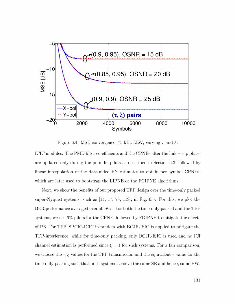
0 2000 4000 6000 8000 10000−20

−15

−10

−5

Symbols

MS

E [dB

]

(τ, ξ) pairs

(0.9, 0.95), OSNR = 15 dB

(0.85, 0.95), OSNR = 20 dB

(0.9, 0.9), OSNR = 25 dB

X−pol

Y−pol

Figure 6.4: MSE convergence, 75 kHz LLW, varying τ and ξ.

ICIC modules. The PMD filter co-efficients and the CPNEs after the link setup phase

are updated only during the periodic pilots as described in Section 6.3, followed by

linear interpolation of the data-aided PN estimates to obtain per symbol CPNEs,

which are later used to bootstrap the LIPNE or the FGIPNE algorithms.

Next, we show the benefits of our proposed TFP design over the time-only packed

super-Nyquist systems, such as [14, 17, 78, 119], in Fig. 6.5. For this, we plot the

BER performance averaged over all SCs. For both the time-only packed and the TFP

systems, we use 6% pilots for the CPNE, followed by FGIPNE to mitigate the effects

of PN. For TFP, SPCIC-ICIC in tandem with BCJR-ISIC is applied to mitigate the

TFP-interference, while for time-only packing, only BCJR-ISIC is used and no ICI

channel estimation is performed since ξ = 1 for such systems. For a fair comparison,

we choose the τ, ξ values for the TFP transmission and the equivalent τ value for the

time-only packing such that both systems achieve the same SE and hence, same BW,

131

20 21 22 23 2410

−6

10−4

10−2

OSNR, dB

BE

R

(0.9,0.9)

(0.84,1)

(0.85,0.95)

(0.82167,1)

169.47 GHz

173.25 GHz

(τ, ξ) pairs

1.1 dB

2.1 dB

Figure 6.5: BER vs. OSNR, highlighting the benefits of the proposed TFP designover time-only packing. 1040 km fiber, 75 kHz LLW, CPNE+FGIPNE, 6% pilotdensity, varying τ and ξ.

with all systems corresponding to 1.2 Tbps data rate. For example, super-Nyquist

WDM systems with τ = 0.9 and ξ = 0.9 corresponds to τ = 0.84 and ξ = 1 to occupy

a BW of 173.25 GHz. For this setting, the proposed TFP system yields a perfor-

mance improvement of 1.1 dB over the time-only packed transmission, as highlighted

in Fig. 6.5. For higher SE values, such gains due to TFP transmission increase. For

example, a TFP (τ, ξ) combination of (0.85, 0.95) offers 2.1 dB OSNR gain over an

equivalent time-packed (0.82167, 1) system that occupies the same BW 169.47 GHz.

The results show that instead of aggressively packing the SCs in one dimension, rela-

tively benign packing in both the temporal and spectral dimensions can be beneficial

when the proposed SPCIC-ICIC together with BCJR-ISIC is employed.

To further quantify the effectiveness of the proposed TFP design, we show the

SE achieved by the proposed TFP systems employing different τ, ξ combinations in

132

0 500 1000 1500 20006.2

6.3

6.4

6.5

6.6

6.7

Distance (km)

SE

(bits/s

/Hz)

(0.87, 1)

(0.82167, 1)(0.85, 0.95)

(0.84, 1)

(0.9, 0.95)(0.9, 0.9)

240−km

960−km

320−km

400−km

160−km

Proposed

[17]

Chap. 5

Chap. 5 with SPCIC

Figure 6.6: SE vs. distance, highlighting the benefits of the proposed TFP designover time-only packing and other TFP designs. 75 kHz LLW, CPNE+FGIPNE, 6%pilot density, varying τ and ξ.

Fig. 6.6, as a function of the transmission distance. For an N -SC DP TFP super-

channel with a code rate Rc, modulation size M , and pilot density p%, we compute

the SE as

SE =2NRc log2M

τ(1 + β) [1 + (N − 1) ξ]

(1− p

100

)bits/s/Hz . (6.13)

In Fig. 6.6, we also include the SE values of the following two benchmark schemes for

reference: (i) the method presented in Chapter 5, employing PIC-ICIC and BCJR-

ISIC with the absence of channel estimation, labeled as “Chap. 5” and (ii) time-

packed ISI-only systems similar to [17] that achieve the same SE. We observe that

a substantial distance improvement of 240− 960 km is achieved by the proposed

technique over (i) mentioned above. Moreover, to show the benefit of the proposed

133

SPCIC over the PIC-based ICIC scheme, we also evaluate the performance of (i) by

replacing the PIC-ICIC with SPCIC, indicated by the legend “Chap. 5 with SPCIC”

in Fig. 6.6, which increases the transmission distance by 240 km for τ = ξ = 0.9,

as highlighted in the figure. Finally, by comparing the proposed TFP systems with

(ii) for the same SE values, we observe a link distance improvement by 2−5 spans

corresponding to 160−400 km for different τ , ξ pairs.

6.6.3 Tolerance to Cascaded ROADMs

While propagating through the optical link, a superchannel signal may be subjected to

additional narrow optical filtering due to multiple network elements, such as cascades

of ROADM nodes implemented by WSSs [118–120]. The effect of such aggressive

filtering manifests itself as severe ISI for the edge SCs of the WDM superchannel as

detailed in Chapter 5. The TFP designs proposed in Chapter 5 applied BCJR-ISIC

for the deterministic TFP-ISI mitigation without adopting any channel estimation

strategy, while the WSS-ISI was countered through the 2×2 linear PMD equalizer.

When a target data rate is intended within a fixed BW, which is dictated by the

effective 3-dB BW of the cascaded WSSs, optimizing the τ, ξ parameters can offer

the best performance under such circumstances, in the form of lowest ROSNR to

attain error-free transmission (see Chapter 5). In this section, we perform a similar

exercise with the considered 1.2 Tbps TFP WDM systems by applying the proposed

interference and PN estimation and cancellation strategies. Our presented design has

the added advantage of the ability to estimate the combined interference stemming

from the TFP transmission and WSS filtering, both of which can be equalized through

the BCJR-ISIC used in conjunction with the proposed SPCIC-ICIC.

For this investigation, we consider 4 WSSs in the 1040 km fiber link, with each

134

18 20 22 24 26 2810

−6

10−4

10−2

100

OSNR, dB

BE

R

1 dB

0 WSS 0.75

dB

2.65 dB

4WSS

166.9 GHz

1.8 dB

Nyquist

Nyquist, Chap. 5

(0.9,0.95), Chap. 5

(0.9,0.9), Proposed

(0.9,0.9), Chap. 5

(0.9,0.95), Proposed

Figure 6.7: BER vs. OSNR, showing tolerance of the proposed scheme to cascadedWSSs. 1040 km fiber, 75 kHz LLW, CPNE+FGIPNE, 6% pilot density, varying τand ξ.

WSS stage modeled as a 6th-order Gaussian filter [118] having a 3-dB BW of 187.5 GHz,

producing an effective 3-dB BW of 166.88 GHz for the cascaded structure. We note

that prior to WSS filtering, the aggregate BW of the Nyquist WDM superchannel

is 206.25 GHz, which can be reduced by enabling a TFP transmission to moderate

the impact of the narrow filtering in order to achieve the same data rate of 1.2 Tbps.

Accounting for the 6% pilot density, spectral restriction by such WSS filtering cor-

responds to an SE value of 6.74 bits/s/Hz. In Fig. 6.7, we plot the average BER of

all SCs as a function of OSNR. The figure indicates that significant gains are offered

by the proposed design over the method presented in Chapter 5 for all combinations

of τ and ξ. For example, OSNR gains of 1 dB and 1.8 dB are highlighted in the

figure corresponding to the Nyquist WDM and the τ =0.9, ξ=0.95 TFP system, re-

spectively. The primary reason for such performance improvement is estimating the

135

20 40 60 80 1000

0.2

0.4

0.6

0.8

LLW (kHz)

RO

SN

R P

enalty (

dB

)

0.2 dB

0.4 dB

0.18

dB

0.15

dB

0.3 dB

Nyquist WDMCPNE−only, 6%

LIPNE, 10 it., 6%

FGIPNE, 10 it., 6%

CPNE−only, 3%

LIPNE, 10 it., 3%

FGIPNE, 10 it., 3%

Figure 6.8: ROSNR penalty vs. LLW for Nyquist WDM, showing benefits andlimitations of CPNE, LIPNE and FGIPNE, having varying pilot densities.

combined effects of the WSS-ISI and the TFP-ISI together, followed by BCJR-ISIC

to counter the overall interference, as opposed to the sub-optimal linear equalization

of the WSS-ISI in Chapter 5. We also note that the optimal TFP parameter combina-

tion remains the same for the proposed TFP design as that in Chapter 5, i.e. τ = 0.9

and ξ = 0.95, which produces an OSNR gain of 2.65 dB over the Nyquist WDM sys-

tem under similar conditions. Additionally, we observe that the performance of the

TFP system with such optimal τ, ξ combination filtered through 4-WSSs is within

0.75 dB of that achieved by the same system without WSS filters in the optical link.

136

50 100 150 200 250 300 350 400

LLW (kHz)

0

0.5

1

1.5

2

OS

NR

Penalty (

dB

)

CPNE-only

LIPNE

"Perfect-decision" CPNE

FGIPNE

Nyquist WDM 1 dB

0.2 dB

(a) Nyquist WDM, i.e. τ = ξ = 1.

50 100 150 200 250 300 350 400

LLW (kHz)

0

0.5

1

1.5

2

OS

NR

Pe

nalty (

dB

)

CPNE-only

LIPNE

"Perfect-decision" CPNE

FGIPNE

= 0.9, = 0.951 dB

0.25 dB

(b) τ = 0.9, ξ = 0.95.

Figure 6.9: ROSNR penalty vs. LLW, showing benefits and limitations of CPNE,LIPNE and FGIPNE, 6% pilot density.

6.6.4 Tolerance to Laser Linewidth

In this section, we present results to show the robustness of the proposed TFP design

against increasing PN levels. First, we study the effect of varying pilot density and

LLW on the proposed CPNE, LIPNE and FGIPNE schemes, for the simplistic case of

a Nyquist WDM system. In Fig. 6.8, we plot the ROSNR penalty of such system over

the benchmark transmission that is not impaired with PN, as a function of the LLW of

the transmitter and the receiver lasers. Both LIPNE and FGIPNE are bootstrapped

with CPNE having 3% and 6% pilot density. Not surprisingly, all PN mitigation

methods produce larger performance degradation with increasing LLW. As shown in

the figure, the gains of LIPNE and FGIPNE over CPNE-only PN mitigation method

also increase with larger LLWs for both pilot densities. The plots in the figure also

suggest that LIPNE is performing close to FGIPNE for LLW up to 100 kHz with a

maximum performance gap of 0.2 dB. Moreover, FGIPNE performs better by 0.15 dB

when it is bootstrapped with CPNE using 6% transmission overhead compared to

3% pilot density.

137

Table 6.2: Computational Complexity.Task Item Number of operations

(Add, Sub., Mul., Div.) per code symbol

Estimation

PMD 12NNw

ISI 14N(Ls + 1)ICI 20N(Lc + 1)

CPNE 14NLIPNE 14N itmax

FGIPNE 2N(17M + 11)itmax

EqualizationISIC O

(4NM

Ls2 itmax

)ICIC O ((M + Lc)N itmax)

After having investigated the performance of the proposed PN cancellation meth-

ods in a Nyquist WDM transmission, we now proceed to evaluate their effectiveness

in TFP systems with even higher values of LLWs. In Fig. 6.9a-6.9b, we plot the

ROSNR penalty over the respective zero-PN systems similar to Fig. 6.8, for the

Nyquist WDM transmission and τ = 0.9,ξ = 0.95 TFP system, respectively. Both

IPNE methods are bootstrapped by the CPNE with 6% pilots. In Fig. 6.9, we

also include the “perfect-decision CPNE” scheme corresponding to the genie-assisted

known transmitted symbols, as a reference. The plots in the figures suggest that

while LIPNE is performing decently compared to FGIPNE for the Nyquist WDM

transmission, FGIPNE outperforms LIPNE by significant margins in TFP systems,

especially when LLW is very high. For example, with 400 kHz LLW, FGIPNE yields

1 dB ROSNR improvement over LIPNE with τ = 0.9, ξ = 0.95 as highlighted in

Fig. 6.9b, whereas such a gain is restricted to only 0.4 dB for the Nyquist trans-

mission as shown in Fig. 6.9a. Moreover, FGIPNE is also able to outperform the

perfect-decision CPNE, and it offers 1 dB gain over “CPNE-only” PN compensation

method for both Nyquist WDM and TFP systems.

138


Details of the computational complexity for the proposed systems design are furnished

in Table 6.2, where M denotes the modulation order, and the rest of the parameters

are already defined in the preceding sections. The numbers in the table correspond

to computations required for both polarizations and all SCs in the superchannel.

As shown, the LMS based estimation algorithms for PMD filter coefficients, TFP

interference and CPNE scale linearly with the number of SCs. Evidently, BCJR-

ISIC constitutes the computationally most challenging module, since the complexity

significantly magnifies with the length of the truncated TFP-ISI channel and the

constellation size [97]. The computational cost of SPCIC-ICIC, however, increases

linearly with the modulation order and TFP-ICI taps length. A comparison between

LIPNE and FGIPNE indicates that FGIPNE exhibits a modulation format depen-

dency, and entails slightly more computations compared to LIPNE, with the benefit

of substantial performance advantage shown in Section 6.6. Moreover, FGIPNE also

requires additional buffering to store the forward and backward FG metrics [70].

6.7 Conclusion

Superchannel data rates of 1 Tbps and more are being targeted in the next gen-

eration optical fiber systems to compete with the increasing demands in network

traffic. To accomplish such target, in this chapter, we proposed flexible designs for

spectrally efficient TFP superchannel transmission achieving Tbps data rates with

significantly higher SE values compared to Nyquist WDM systems. For this, we have

presented sophisticated signal processing tools to efficiently handle TFP interference

and accomplish CPR. Our simulation results suggest that by employing the proposed

139

interference channel and PN estimation methods, together with the BCJR-ISIC and

the novel SPCIC-ICIC scheme, the presented TFP WDM systems offer more than

2 dB ROSNR gains and 160−400 km transmission distance improvements over state-

of-the-art super-Nyquist superchannel transmission techniques. The proposed DSP

design shows outstanding tolerance to PN with LLW up to 400 kHz. Moreover, our

system exhibits excellent robustness against additional aggressive optical filtering in

the form of cascades of ROADM nodes comprised of narrow WSS filters that may be

present in the longhaul fiber link.

140

Chapter 7

Concluding Remarks & Future

Directions

7.1 Summary and Conclusions

FTN signaling is a spectrally efficient technology that can facilitate high data rates

in the bandwidth-starved existing fixed transmission networks, which serve as the

backbone for the Internet and the mobile data traffic. The communication links for

such networks are primarily comprised of optical fibers and point-to-point microwave

radio. In this thesis, we investigated the application of FTN signaling in these OFC

and MWC links by taking necessary measures to tackle the interference introduced

by FTN, together with the consideration of other practical challenges present in these

systems. Based on the current deployment of the existing fixed transmission network

infrastructure, we broadly considered three application scenarios, namely (a) single

carrier DP OFC systems, (b) single carrier DP MWC systems, and (c) multicarrier

DP OFC systems, for introducing and evaluating the concept of FTN signaling.

Firstly, we considered FTN transmission of a DP COSC system. Against the

backdrop of the existing literature, which predominantly employs computationally

complex and buffer-space constrained receiver-side equalization strategies to mitigate

the FTN-ISI, in this thesis, we adopted an alternative approach of pre-equalizing the

ISI at the transmitter. For this, we began with the application of the well-known non-

141

linear precoding method THP, and designed novel, cost-efficient soft demappers to

reduce the impact of the modulo-loss, which incurs severe performance degradation

in COSC systems employing traditional THP-demappers. Moreover, we presented

a linear precoding technique LPE that achieved the optimal BER performance by

orthogonalizing the FTN-ISI channel, and thereby, making such precoding scheme

competitive to computationally expensive BCJR-based MAP equalization. Numeri-

cal results for a precoded COSC system suggested significant performance and com-

plexity gains of the proposed precoding schemes over state-of-the-art methods.

Secondly, we applied FTN signaling in a point-to-point microwave link employing

HoM formats and polarization multiplexing. In addition to the FTN-ISI, such DP

systems suffer from multiple additional practical challenges, in the form of multipath-

ISI, PN and XPI. While the polarization cross-talk in OFC systems can be perfectly

equalized by employing proper linear filters, the application of FTN signaling and

HoM formats in MWC systems complicates the XPI mitigation. In this thesis, DP-

FTN HoM systems were introduced for the first time. For this, we presented power-

ful, and yet computationally simple, signal processing algorithms to jointly equalize

or pre-equalize the aggregate interference stemming from the mutipath reflections,

FTN signaling and polarization multiplexing, in tandem with CPR via suitable PN

mitigation techniques. Our numerical results for an MWC transmission established

significant performance advantage in favor of FTN signaling over equivalent Nyquist

systems. For example, the newly designed DP-FTN systems empowered with the

proposed DSP algorithms offered as high as 5.5 dB performance improvement over a

Nyquist transmission that employed a higher modulation order to achieve the same

data rate.

Thirdly, we considered MFTN OFC systems in the form of TFP WDM superchan-

142

nels. Since the practical limitations of the opto-electronics preclude the feasibility

of facilitating single carrier transmission with very high baud rates, TFP WDM su-

perchannels are useful to achieve high throughputs. We began with the application

of precoding in TFP superchannels, as an alternative to complicated receiver-side

equalization. For this, we presented pre-equalization schemes at the transmitter to

mitigate, jointly or otherwise, the ISI and ICI stemming from the TFP transmission.

In this thesis, precoded MFTN systems enabling packing of symbols in both time

and frequency dimensions were introduced for the first time. Simulation results for

the such systems established considerable gains by the proposed methods over com-

petitive equalization schemes having similar or higher computational complexity. To

keep up with the futuristic targets set for the next generation optical networks, we

then considered spectrally efficient TFP superchannels achieving Tbps data rates,

packed within a target aggregate BW. For this, we noticed that the functionality

of the proposed precoding methods was limited to a restricted range of time and

frequency compression. Therefore, to achieve higher SE, we turned our focus on

the existing receiver-side turbo equalization methods present in the literature under

the premises of an AWGN channel, and tailored them to the considered OFC sys-

tems. Thereafter, we presented more flexible and high-performance DSP designs for

the TFP Terabit-superchannels, by jointly estimating the TFP-ISI and ICI channels,

coupled with sophisticated CPR and scheduling algorithms. The presented numerical

results indicated that the proposed spectrally efficient Tbps systems offered signif-

icant transmission distance improvement over existing super-Nyquist designs, and

exhibited excellent tolerance to high LLWs and aggressive optical filtering stemming

from the cascades of ROADM nodes.

In conclusion, we have demonstrated that FTN signaling empowered with the

143

proposed signal processing algorithms in this thesis bears significant merit to meet

and exceed the high SE and throughput requirements set for the future generation

fixed transmission networks. However, to accomplish the SE improvements over

Nyquist transmission, FTN systems require additional computational complexity.

The numerical results presented in this thesis not only validated the effectiveness of

the proposed algorithms, but also established substantial superiority of the proposed

schemes over state-of-the-art designs.

7.2 Future Work

In the final portion of this dissertation, we present potential avenues for future re-

search.

7.2.1 FTN and Probabilistic Shaping

In this thesis, we have shown that FTN signaling is an efficient means to obtain higher

SE. To achieve further SE improvements in the optical links, other technologies can

also be applied, as an alternative to, or in conjunction with FTN. For example, prob-

abilistic shaping [79, 127, 129, 132, 133] employing HoM formats in OFC systems is

considered to be another interesting research direction that has attracted renewed

interest lately. Such systems provide shaping gains by assigning non-uniform proba-

bilities to the signal constellation points, at the price of increased sensitivity to PN

and fiber nonlinearity [129, 133]. Investigating whether FTN/TFP systems equipped

with our proposed DSP design serves as a competitive or complementary technol-

ogy to probabilistically shaped optical transmission is an attractive future research

avenue worth pursuing.

144

7.2.2 Fiber Nonlinearity

Fiber nonlinearity stemming from Kerr effects incurs severe performance degradation

in practical OFC systems when the launch power is high [134]. Consequently, for such

systems, nonlinear effects restrict the application of HoM formats, which operate in

the high OSNR regime. In this thesis, the optical launch powers considered for our

simulations were set at sufficiently low values where the effects of fiber nonlinearity

are negligible. However, it will be interesting to know how the performance of the

proposed TFP transmission is affected in the presence of nonlinearity in a more real-

istic OFC link, with or without nonlinear compensation techniques integrated with

the receiver DSP. It is also noteworthy to mention that part of the fiber nonlinearity

manifests itself as a nonlinear PN [133, 134]. Therefore, future research efforts may

be directed towards investigating whether the iterative CPR algorithms we presented

in Chapter 6 of this thesis for TFP systems are capable of eliminating such PN.

7.2.3 Additional Device Non-idealities and Impairments

In the numerical evaluation of the proposed algorithms for the OFC and the MWC

systems, we have assumed perfect time and frequency synchronization. However,

timing offset and carrier frequency offset introduced by imperfect radio-frequency

and opto-electronic transceiver components (e.g., LOs, lasers, etc.) can severely

restrict the performance of the communication links. Other non-idealities that were

also ignored in the simulations were power amplifier nonlinearities in MWC systems,

DAC and ADC quantization noise, and I/Q gain and phase imbalances, which may

require additional DSP algorithms for their mitigation. Evaluating the proposed

methods in the presence of such impairments is left here as a future work.

145

Bibliography

[1] “Backhaul Alternatives for HetNet Small Cells,” Business Intelligence Division,

Informa PLC, Tech. Rep., September 2015.

[2] “Cisco Visual Networking Index: Forecast and Methodology, 2017–2022,”

Cisco, Tech. Rep., February 2019.

[3] “Cisco Visual Networking Index: Global Mobile Data Traffic Forecast Update,

2017–2022,” Cisco, Tech. Rep., February 2019.

[4] “Ericsson Microwave Outlook Report 2017,” Ericsson, Tech. Rep., December

2017.

[5] R. Essiambre, G. Kramer, P. Winzer, G. Foschini, and B. Goebel, “Capacity

Limits of Optical Fiber Networks,” J. Lightw. Technol., vol. 28, no. 4, pp.

662–701, February 2010.

[6] “Ericsson Microwave Outlook Report 2018,” Ericsson, Tech. Rep., December

2018.

[7] J. E. Mazo, “Faster-than-Nyquist Signaling,” Bell Syst. Tech. J., vol. 54, no. 8,

pp. 1451–1462, October 1975.

[8] J. E. Mazo and H. J. Landau, “On the Minimum Distance Problem for Faster-

than-Nyquist Signaling,” IEEE Trans. Inf. Theory, vol. 34, no. 6, pp. 1420–

1427, November 1988.

146

[9] D. Hajela, “On Computing the Minimum Distance for Faster than Nyquist

Signaling,” IEEE Trans. Inf. Theory, vol. 36, no. 2, pp. 289–295, March 1990.

[10] J. B. Anderson, F. Rusek, and V. Owall, “Faster-Than-Nyquist Signaling,” in

Proc. IEEE, vol. 101, no. 8, 2013, pp. 1817–1830.

[11] G. Colavolpe, T. Foggi, A. Modenini, and A. Piemontese, “Faster-than-Nyquist

and beyond: how to improve spectral efficiency by accepting interference,”

Optics Express, vol. 19, no. 27, pp. 26 600–26 609, December 2000.

[12] A. D. Liveris and C. N. Georghiades, “Exploiting Faster-than-Nyquist Signal-

ing,” IEEE Trans. Commun., vol. 51, no. 9, pp. 1502–1511, September 2003.

[13] F. Rusek, “Partial Response and Faster-than-Nyquist Signaling,” Ph.D. disser-

tation, Lund University, 2007.

[14] G. Colavolpe and T. Foggi, “Time-Frequency Packing for High-Capacity Co-

herent Optical Links,” IEEE Trans. on Commun., vol. 62, no. 8, pp. 2986–2995,

August 2014.

[15] K. Roberts et al., “High Capacity Transport - 100G and Beyond,” J. Lightw.

Technol, vol. 33, no. 3, pp. 563–578, February 2015.

[16] S. Chen et al., “Comparison of Advanced Detection Techniques for QPSK Sig-

nals in Super-Nyquist WDM Systems,” IEEE Photon. Technol. Lett., vol. 27,

no. 1, pp. 105–108, January 2015.

[17] M. Secondini, T. Foggi et al., “Optical Time-Frequency Packing: Principles,

Design, Implementation, and Experimental Demonstration,” J. Lightw. Tech-

nol, vol. 33, no. 17, pp. 3558–3570, September 2015.

147

[18] Z. Xiao et al., “ICI Mitigation for Dual-Carrier Superchannel Transmission

Based on m-PSK and m-QAM Formats,” J. Lightw. Technol, vol. 34, no. 23,

pp. 5526–5533, December 2016.

[19] J. Pan et al., “Inter-Channel Crosstalk Cancellation for Nyquist-WDM Su-

perchannel Applications,” J. Lightw. Technol, vol. 30, no. 24, pp. 3593–3999,

December 2012.

[20] K. Shibahara et al., “Multi-stage Successive Interference Cancellation for

Spectrally-Efficient Super-Nyquist Transmission,” in European Conf. on Opt.

Commun. (ECOC), 2015, pp. 1–3.

[21] Q. Hu et al., “Inter-Channel Crosstalk Compensation for Time-Frequency Pack-

ing Systems,” in European Conf. on Opt. Commun. (ECOC), 2017, pp. 1–3.

[22] P. Noel, M. Prokoptsov, M. Klemes, H. Tai, A. Dufour, and K. Morris, “The

Design, Development and Implementation of a Cross-polarization Interference

Cancellation System for Point-to-point Digital Microwave Radio systems,” in

IEEE Canadian Conf. on Elec. and Comp. Engg. (CCECE), 2011.

[23] P. Noel and M. Klemes, “Doubling the Through-Put of a Digital Microwave

Radio System by the Implementation of a Cross-Polarization Interference Can-

cellation Algorithm,” in IEEE Radio and Wireless Symp. (RWS), 2012.

[24] B. Lankl, A. Nist, J. A. Nossek, and G. Sebald, “Fully Digital ATDE’s and

XPIC’s for a STM-1 Cochannel Radio System Family,” in IEEE Int. Conf. on

Commun. (ICC), 1989.

[25] K. W. Suh, C. Y. Park, G. Y. Hur, and D. Y. Lee, “A Powerful 13-Tap ATDE

148

and XPIC Implemented on One Chip for Co-channel Digital Radio System,”

in IEEE National Telesys. Conf., 1994.

[26] H. Proenca and N. B. Carvalho, “Cross-Polarization Interference Cancelation

(XPIC) Performance in Presence of Non-linear Effects,” in IEEE Workshop on

Int. Nonlin. MW and mm-Wave Circ. (INMMIC), 2010.

[27] R. Valentin, H. G. Giloi, and K. Metzger, “Performance of Digital Radio

Systems in Co-channel Cross-polarized Operation,” in IEEE Global Commun.

Conf. (GLOBECOM), 1991.

[28] M. Kavehrad, “Baseband Cross-Polarization Interference Cancellation for M-

Quadrature Amplitude Modulated Signals Over Multipath Fading Radio Chan-

nels,” AT&T Tech. J., vol. 64, no. 8, pp. 1913–1926, October 1985.

[29] T. Ingason, H. Liu, M. Coldrey, A. Wolfgang, and J. Hansryd, “Impact of Fre-

quency Selective Channels on a Line-of-Sight MIMO Microwave Radio Link,”

in IEEE Vehicular Tech. Conf. Spring (VTC), 2010.

[30] M. Martalo, G. Ferrari, M. Asim, J. Gambini, C. Mazzucco, G. Cannalire,

S. Bianchi, and R. Raheli, “Iterative Synchronization for Dually-Polarized In-

dependent Transmission Streams,” IEEE Trans. Commun., vol. 65, no. 6, pp.

2534–2542, June 2017.

[31] ——, “Phase noise Compensation for Dually-polarized Systems with Indepen-

dent Transmission Streams,” in IEEE Int. Symp. on Wireless Commun. Sys.

(ISWCS), 2015.

[32] A. Vizziello, P. Savazzi, and R. Borra, “Joint Phase Recovery for XPIC System

149

Exploiting Adaptive Kalman Filtering,” IEEE Commn. Lett., vol. 20, no. 5,

pp. 922–925, May 2016.

[33] M. Seimetz, High-Order Modulation for Optical Fiber Transmission. Springer

Berlin Heidelberg, 2010.

[34] Y. Baeyens, S. Shahramian, B. Jalali, P. Roux, J. Weiner, A. Singh, M. Moretto,

P. Boutet, and P. Lopez, “A Wideband SiGe BiCMOS Transceiver Chip-set for

High-performance Microwave Links in the 5.643.5 GHz Range,” in IEEE Radio

Freq. Int. Circ. Symp. (RFIC), 2017.

[35] A. Prlja, J. B. Anderson, and F. Rusek, “Receivers for Faster-than-Nyquist

Signaling with and without Turbo Equalization,” in IEEE Int. Symp. on Inf.

Theory, 2008, pp. 464–468.

[36] A. Prlja and J. B. Anderson, “Reduced-Complexity Receivers for Strongly Nar-

rowband Intersymbol Interference Introduced by Faster-than-Nyquist Signal-

ing,” IEEE Trans. Commun., vol. 60, no. 9, pp. 2591–2601, September 2012.

[37] F. Rusek and J. B. Anderson, “Successive Interference Cancellation in Mul-

tistream Faster-than-Nyquist Signaling,” in Int. Conf. on Wireless Commun.

and Mobile Computing, 2006, pp. 1021–1026.

[38] J. Yu, J. Park, F. Rusek, B. Kudryashov, and I. Bocharova, “High Order Mod-

ulation in Faster-Than-Nyquist Signaling Communication Systems,” in IEEE

Vehicular Tech. Conf. Fall (VTC), 2014.

[39] S. Sugiura, “Frequency-Domain Equalization of Faster-than-Nyquist Signal-

ing,” IEEE Wireless Commun. Lett., vol. 2, no. 5, pp. 555–558, October 2013.

150

[40] S. Sugiura and L. Hanzo, “Frequency-Domain-Equalization-Aided Iterative De-

tection of Faster-than-Nyquist Signaling,” IEEE Trans. Veh. Technol., vol. 64,

no. 5, pp. 2122–2128, May 2015.

[41] T. Ishihara and S. Sugiura, “Frequency-Domain Equalization Aided Iterative

Detection of Faster-than-Nyquist Signaling with Noise Whitening,” in IEEE

Int. Conf. on Commun. (ICC), 2016, pp. 1–6.

[42] M. Tomlinson, “New Automatic Equaliser Employing Modulo Arithmetic,”

Electronics Letters, vol. 7, no. 5, pp. 138–139, March 1971.

[43] H. Harashima and H. Miyakawa, “Matched-Transmission Technique for Chan-

nels with Intersymbol Interference,” IEEE Trans. Commun., vol. 20, no. 4, pp.

774–780, August 1972.

[44] R. F. H. Fischer, Precoding and Signal Shaping for Digital Transmission.

Wiley-IEEE Press, 2002.

[45] M. E. Hefnawy and H. Taoka, “Overview of Faster-Than-Nyquist for Fu-

ture Mobile Communication Systems,” in IEEE Vehicular Tech. Conf. Spring

(VTC), 2013.

[46] F. L. Luo and C. Zhang, Signal Processing for 5G: Algorithms and Implemen-

tations. Wiley-IEEE Press, 2016.

[47] M. Maso and S. Tomasin, “Pre-equalized Faster Than Nyquist Transmission

for 5G Cellular Cicrowave Back-haul,” in IEEE Int. workshop on Signal Proc.

advances in Wireless Commun. (SPAWC), 2016.

[48] D. Chang, O. Omomukuyo, O. Dobre, R. Venkatesan, P. Gillard, and C. Rum-

bolt, “Tomlinson-Harashima Precoding with Soft Detection for Faster than

151

Nyquist DP-16QAM Coherent Optical Systems,” in Opt. Fiber Commun.

Conf.(OFC), 2015, pp. 1–3.

[49] D. Chang, O. Omomukuyo, X. Lin, S. Zhang, O. Dobre, and V. Ramachan-

dran, “Robust Faster-than-Nyquist PDM-mQAM Systems with Tomlinson-

Harashima Precoding,” IEEE Photon. Technol. Lett., vol. 28, no. 19, October

2016.

[50] R. Rath and W. Rosenkranz, “Tomlinson-Harashima Precoding for Fiber-Optic

Communication Systems,” in European Conf. on Opt. Commun. (ECOC), 2013,

pp. 1–3.

[51] R. Rath, C. Schmidt, and W. Rosenkranz, “Is Tomlinson-Harashima Precoding

Suitable for Fiber-Optic Communication Systems?” in ITG Symp. on Phot.

Networks, 2013, pp. 1–7.

[52] E. C. Y. Peh and Y. C. Liang, “Power and modulo loss tradeoff with expanded

soft demapper for LDPC coded GMD-THP MIMO systems,” IEEE Trans.

Wireless Commun., vol. 8, no. 2, pp. 714–724, February 2009.

[53] S. Kinjo, “An Efficient Soft Demapper for Tomlinson-Harashima Precoded Sys-

tems,” IEICE Comm. Exp., vol. 4, no. 3, pp. 89–94, March 2015.

[54] E. Kaminer, D. Raphaeli, and Y. Hayoun, “Iterative Decoding of Coded THP

with Quantized Output,” IEEE Trans. Commun., vol. 61, no. 9, pp. 3721–3729,

September 2013.

[55] A. Said and J. Anderson, “Bandwidth-Efficient Coded Modulation with Op-

timized Linear Partial-Response Signals,” IEEE Trans. Inf. Theory, vol. 44,

no. 2, pp. 701–713, March 1998.

152

[56] F. Rusek and J. B. Anderson, “Non Binary and Precoded Faster Than Nyquist

Signaling,” IEEE Trans. Commun., vol. 56, no. 5, pp. 808–817, May 2008.

[57] Y. J. D. Kim and J. Bajcsy, “On Spectrum Broadening of Pre-Coded Faster-

Than-Nyquist Signaling,” in IEEE Vehicular Tech. Conf. Fall (VTC), 2010,

pp. 1–5.

[58] E. Ringh, “Low Complexity Algorithms for Faster-than-Nyquist Signalling :

Using Coding to Avoid an NP-hard Problem,” Master’s thesis, KTH Royal

Institute of Technology: School of Engineering Sciences, 2013.

[59] A. Gattami, E. Ringh, and J. Karlsson, “Time Localization and Capacity of

Faster-Than-Nyquist Signaling,” in IEEE Global Commun. Conf. (GLOBE-

COM), 2015, pp. 1–7.

[60] G. Colavolpe, T. Foggi, E. Forestieri, and G. Prati, “Robust Multilevel Co-

herent Optical Systems With Linear Processing at the Receiver,” J. Lightw.

Technol, vol. 27, no. 13, pp. 2357–2369, July 2009.

[61] W. D. Rummler, “A New Selective Fading Model: Application to Propagation

Data,” Bell Syst. Tech. J., vol. 58, no. 5, pp. 1037–1071, May 1979.

[62] H. Mehrpouyan, A. A. Nasir, S. D. Blostein, T. Eriksson, G. K. Karagiannidis,

and T. Svensson, “Joint Estimation of Channel and Oscillator Phase Noise in

MIMO Systems,” IEEE Trans. Signal Process., vol. 60, no. 9, pp. 4790–4807,

September 2012.

[63] T. Ishihara and S. Sugiura, “Iterative Frequency-Domain Joint Channel Esti-

mation and Data Detection of Faster-Than-Nyquist Signaling,” IEEE Trans.

Wireless Commun., vol. 16, no. 9, pp. 6221–6231, September 2017.

153

[64] Q. Shi, N. Wu, X. Ma, and H. Wang, “Frequency-Domain Joint Channel Esti-

mation and Decoding for Faster-Than-Nyquist Signaling,” IEEE Trans. Com-

mun., vol. 66, no. 2, pp. 781–795, February 2018.

[65] E. Bedeer, M. H. Ahmed, and H. Yanikomeroglu, “Low-Complexity Detection

of High-Order QAM Faster-Than-Nyquist Signaling,” IEEE Access, vol. 5, pp.

14 579–14 588, 2017.

[66] W. Yuan, N. Wu, H. Wang, and J. Kuang, “Variational Inference-Based

Frequency-Domain Equalization for Faster-Than-Nyquist Signaling in Doubly

Selective Channels,” IEEE Signal Process. Lett., vol. 23, no. 9, pp. 1270–1274,

September 2016.

[67] D. D. Lin, R. A. Pacheco, T. J. Lim, and D. Hatzinakos, “Joint Estimation

of Channel Response, Frequency Offset, and Phase Noise in OFDM,” IEEE

Trans. Signal Process., vol. 54, no. 9, pp. 3542–3554, September 2006.

[68] X. Qi, N. Wu, H. Wang, and W. Yuan, “A Factor Graph-Based Iterative De-

tection of Faster-than-Nyquist Signaling in the Presence of Phase Noise and

Carrier Frequency Offset,” DSP, vol. 63, pp. 25–34, April 2017.

[69] X. Qi, N. Wu, L. Zhou, D. Yang, and H. Wang, “Joint Phase Noise Estima-

tion and Iterative Detection of Faster-than-Nyquist Signaling Based on Factor

Graph,” in IEEE Vehicular Tech. Conf. Spring (VTC), 2017.

[70] G. Colavolpe, A. Barbieri, and G. Caire, “Algorithms for Iterative Decoding

in the Presence of Strong Phase Noise,” IEEE J. Sel. Areas Commun., vol. 23,

no. 9, pp. 1748–1757, September 2005.

154

[71] A. Barbieri, G. Colavolpe, and G. Caire, “Joint Iterative Detection and De-

coding in the Presence of Phase Noise and Frequency Offset,” IEEE Trans.

Commun., vol. 55, no. 1, pp. 171–179, January 2007.

[72] N. Al-Dhahir and A. H. Sayed, “The Finite-Length Multi-Input Multi-Output

MMSE-DFE,” IEEE Trans. Signal Process., vol. 48, no. 10, pp. 2921–2936,

October 2000.

[73] R. Merched and N. R. Yousef, “Fast Techniques for Computing Finite-Length

MIMO MMSE Decision Feedback Equalizers,” IEEE Trans. Signal Process.,

vol. 54, no. 2, pp. 701–711, February 2006.

[74] A. M. Tehrani, B. Hassibi, and J. M. Cioffi, “Adaptive Equalization of Multiple-

Input Multiple-Output (MIMO) Channels,” in IEEE Int. Conf. on Commun.

(ICC), 2000.

[75] D. Falconer, “Application of Passband Decision Feedback Equalization in Two-

Dimensional Data Communication Systems,” IEEE Trans. Commun., vol. 24,

no. 10, pp. 1159–1166, October 1976.

[76] S. Moridi and H. Sari, “Analysis of Four Decision-Feedback Carrier Recovery

Loops in the Presence of Intersymbol Interference,” IEEE Trans. Commun.,

vol. 33, no. 6, pp. 543–550, June 1985.

[77] A. Stark and D. Raphaeli, “Combining Decision-Feedback Equalization and

Carrier Recovery for Two-Dimensional Signal Constellations,” IEEE Trans.

Commun., vol. 55, no. 10, pp. 2012–2021, October 2007.

[78] G. Meloni, T. Rahman et al., “Experimental Comparison of Transmission Per-

155

formance for Nyquist WDM and Time-Frequency Packing,” J. Lightw. Technol,

vol. 33, no. 24, pp. 5261–5268, December 2015.

[79] L. Li, Z. Xiao, L. Liu, and Y. Lu, “Non-Orthogonal WDM Systems with Faster

than Nyquist Technology,” in Opt. Fiber Commun. Conf.(OFC), 2019, pp. 1–3.

[80] D. Dasalukunte, “Multicarrier Faster-than-Nyquist Signaling Transceivers,”

Ph.D. dissertation, Lund University, 2012.

[81] A. Barbieri et al., “Time-frequency Packing for Linear Modulations: Spec-

tral Efficiency and Practical Detection Schemes,” IEEE Trans. on Commun.,

vol. 57, no. 10, pp. 2951–2959, October 2009.

[82] T. Pfau, S. Hoffmann, and R. Noe, “Hardware-Efficient Coherent Digital Re-

ceiver Concept With Feedforward Carrier Recovery for M-QAM Constella-

tions,” J. Lightw. Technol, vol. 27, no. 8, pp. 989–999, April 2009.

[83] M. P. Yankov, T. Fehenberger, L. Barletta, and N. Hanik, “Low-Complexity

Tracking of Laser and Nonlinear Phase Noise in WDM Optical Fiber Systems,”

J. Lightw. Technol, vol. 33, no. 23, pp. 4975–4984, December 2015.

[84] J. C. M. Diniz et al., “Low-complexity Carrier Phase Recovery Based on Prin-

cipal Component Analysis for Square-QAM Modulation Formats,” Optics Ex-

press, vol. 27, no. 11, pp. 15 617–15 626, May 2019.

[85] J. Hald, L. Nielsen, J. C. Petersen, P. Varming, and J. E. Pedersen, “Fiber

Laser Optical Frequency Standard at 1.54 m,” Optics Express, vol. 19, no. 3,

pp. 2052–2063, January 2011.

[86] K. Balskus et al., “Frequency Comb Metrology with an Optical Parametric

Oscillator,” Optics Express, vol. 24, no. 8, pp. 8370–8381, April 2016.

156

[87] M. Jana, A. Medra, L. Lampe, and J. Mitra, “Precoded Faster-than-

Nyquist Coherent Optical Transmission,” in European Conf. on Opt. Commun.

(ECOC), 2016.

[88] ——, “Pre-equalized Faster-than-Nyquist Transmission,” IEEE Trans. Com-

mun., vol. 65, no. 10, pp. 4406–4418, October 2017.

[89] M. Jana, L. Lampe, and J. Mitra, “Interference and Phase Noise Mitigation in

a Dual-Polarized Faster-than-Nyquist Trasnmission,” in IEEE Int. Workshop

on Signal Proc. advances in Wireless Commun. (SPAWC), 2018.

[90] ——, “Dual-polarized Faster-than-Nyquist Transmission Using Higher-order

Modulation Schemes,” IEEE Trans. Commun., vol. 66, no. 11, pp. 5332–5345,

November 2018.

[91] ——, “Precoded Time-Frequency-Packed Multicarrier Faster-than-Nyquist

Transmission,” in IEEE Int. workshop on Signal Proc. advances in Wireless

Commun. (SPAWC), 2019.

[92] ——, “Interference Cancellation for Time-Frequency Packed Super-Nyquist

WDM Systems,” IEEE Photon. Technol. Lett., vol. 30, no. 24, pp. 2099–2102,

December 2018.

[93] ——, “Spectrally Efficient Time-Frequency Packed WDM Superchannel Trans-

mission,” To be submitted in IEEE Trans. Commun., 2019.

[94] R. F. H. Fischer, “Sorted Spectral Factorization of Matrix Polynomials in

MIMO Communications,” IEEE Trans. Commun., vol. 53, no. 6, pp. 945–951,

June 2005.

157

[95] A. Papoulis and S. U. Pillai, Probability, Random Variables and Stochastic

Processes. Tata McGraw-Hill, 2002.

[96] E. Ip and J. M. Kahn, “Digital Equalization of Chromatic Dispersion and

Polarization Mode Dispersion,” J. Lightw. Technol, vol. 25, no. 8, pp. 2033–

2043, August 2007.

[97] D. Wang and H. Kobayashi, “Matrix Approach for Fast Implementations of

Logarithmic MAP Decoding of Turbo Codes,” in IEEE Pacific Rim Conf. on

Commun.,Compt. and Signal Proc., 2001, pp. 115–118.

[98] A. Demir, A. Mehrotra, and J. Roychowdhury, “Phase noise in Oscillators: A

Unifying Theory and Numerical Methods for Characterization,” IEEE Trans.

Circuits Syst. I, Fundam. Theory Appl., vol. 47, no. 5, pp. 655–674, May 2000.

[99] N. Kamiya and E. Sasaki, “Pilot-Symbol Assisted and Code-Aided Phase Er-

ror Estimation for High-Order QAM Transmission,” IEEE Trans. Commun.,

vol. 61, no. 10, pp. 4369–4380, October 2013.

[100] A. Spalvieri and L. Barletta, “Pilot-Aided Carrier Recovery in the Presence of

Phase Noise,” IEEE Trans. Commun., vol. 59, no. 7, pp. 1966–1974, July 2011.

[101] G. Milotta and A. Carugati, “Communication Between Modems in XPIC

Configuration for Wireless Applications ,” Patent US8 615 055 B2, December,

2013. [Online]. Available: http://www.google.com/patents/US8615055

[102] D. D. Falconer, “Jointly adaptive equalization and carrier recovery in two-

dimensional digital communication systems,” Bell Syst. Tech. J., vol. 55, no. 3,

pp. 317–334, March 1976.

158

[103] J. Proakis and M. Salehi, Digital Communications. McGraw-Hill Education,

2007.

[104] S. Haykin, Adaptive Filter Theory. New Jersy: Prentice-Hall, 1986.

[105] M. Umari, “Effect of Colored Noise on the Performance of LMS Adaptive Equal-

izers and Predictors,” in IEEE Int. Symp. on Circ. and Sys. (ISCAS), 1992.

[106] M. Reuter and J. Zeidler, “Nonlinear Effects in LMS Adaptive Equalizers,”

IEEE Trans. Signal Process., vol. 47, no. 6, pp. 1570–1579, June 1999.

[107] N. Al-Dhahir and J. Cioffi, “MMSE Decision-Feedback Equalizers: Finite-

length Results,” IEEE Trans. Inf. Theory, vol. 41, no. 4, pp. 961–975, July

1995.

[108] F. Rusek and J. B. Anderson, “Constrained Capacities for Faster-Than-Nyquist

Signaling,” IEEE Trans. Inf. Theory, vol. 55, no. 2, pp. 764–775, February 2009.

[109] Digital Video Broadcasting (DVB); Second generation framing structure,

channel coding and modulation systems for Broadcasting, Interactive Services,

News Gathering and other broadband satellite applications (DVB-S2), ETSI

EN 302 307 V1.2.1 Std. [Online]. Available: www.dvb.org/standards/dvb-s2

[110] H. Ge, “Investigation of LDPC code in DVB-S2,” Master’s thesis, Linkoping

University, Dept. of Electrical Engineering, 2012.

[111] B. Lankl, J. Nossek, and G. Sebald, “Cross-polarization Interference Cancella-

tion in the Presence of Delay Effects,” in IEEE Int. Conf. on Commun. (ICC),

1988.

159

[112] S. Peng, A. Liu, K. Wang, and X. Liang, “PAPR Reduction of Multicarrier

Faster-Than-Nyquist Signals With Partial Transmit Sequence,” IEEE Access,

vol. 5, pp. 24 931–24 937, 2017.

[113] P. Banelli, S. Buzzi, G. Colavolpe, A. Modenini, F. Rusek, and A. Ugolini,

“Modulation formats and waveforms for 5G networks: Who will be the heir of

OFDM?” IEEE Sig. Proc. Magazine, vol. 31, no. 6, pp. 80–93, November 2014.

[114] K.Shibahara, A. Masuda, S. Kawai, and M. Fukutoku, “Multi-stage Successive

Interference Cancellation for Spectrally-Efficient Super-Nyquist Transmission,”

in European Conf. on Opt. Commun. (ECOC), 2015, pp. 1–3.

[115] R. Fischer, “Sorted Spectral Factorization of Matrix Polynomials in MIMO

Communications,” IEEE Trans. on Commun., vol. 53, no. 6, pp. 945–951, June

2005.

[116] D. Youla and N. Kazanjian, “Bauer-Type Factorization of Positive Matrices

and the Theory of Matrix Polynomials Orthogonal on the Unit Circle,” IEEE

Trans. on Circuits and Sytems, vol. 25, no. 2, pp. 57–69, February 1978.

[117] A. Barbieri, D. Fertonani, and G. Colavolpe, “Time-frequency Packing for Lin-

ear Modulations: Spectral Efficiency and Practical Detection Schemes,” IEEE

Trans. on Commun., vol. 57, no. 10, pp. 2951–2959, October 2009.

[118] T. Strasser et al., “Wavelength-Selective Switches for ROADM Applications,”

IEEE J. Sel. Topics Quantum Electron., vol. 16, no. 5, pp. 1150–1157, Septem-

ber 2010.

[119] T. Foggi et al., “Spectral Efficiency Optimization in Flexi-Grid Long-Haul Op-

tical Systems,” J. Lightw. Technol, vol. 33, no. 13, pp. 2735–2742, July 2015.

160

[120] D. Marom et al., “Survey of Photonic Switching Architectures and Technologies

in Support of Spatially an Spectrally Flexible Optical Networking [Invited],”

IEEE J. Opt. Commun. Netw., vol. 9, no. 1, pp. 1–26, January 2017.

[121] F. Rusek and J. B. Anderson, “Multistream Faster than Nyquist Signaling,”

IEEE Trans. Commun., vol. 57, no. 5, pp. 1329–1340, May 2009.

[122] C. Xie and X. Zhou, Enabling Technologies for High Spectral-efficiency Coherent

Optical Communication Networks. John Wiley & Sons, Inc, 2016.

[123] M. P. Yankov, T. Fehenberger, L. Barletta, and N. Hanik, “Low-Complexity

Tracking of Laser and Nonlinear Phase Noise in WDM Optical Fiber Systems,”

J. Lightw. Technol, vol. 33, no. 23, pp. 4975–4984, December 2015.

[124] M. A. Reimer, “Simulation Methods for the Temporal and Frequency Dynamics

of Optical Communication Systems,” Ph.D. dissertation, The University of

Waterloo, 2012.

[125] F. Rusek, M. Loncar, and A. Prlja, “A Comparison of Ungerboeck and Forney

Models for Reduced-Complexity ISI Equalization,” in IEEE Global Commun.

Conf. (GLOBECOM), 2007, pp. 1431–1437.

[126] G. Colavolpe and A. Barbieri, “On MAP symbol detection for ISI channels

using the Ungerboeck observation model,” IEEE Commun. Lett., vol. 9, no. 8,

pp. 720–722, August 2005.

[127] G. Bosco, “Advanced Modulation Techniques for Flexible Optical Transceivers:

The Rate/Reach Tradeoff,” J. Lightw. Technol, vol. 37, no. 1, pp. 36–49, Jan-

uary 2019.

161

[128] S. Makovejs et al., “Characterization of Long-haul 112Gbit/s PDM-QAM-16

Transmission with and without Digital Nonlinearity Compensation,” Optics

Express, vol. 18, no. 12, pp. 12 939–12 947, June 2010.

[129] T. Fehenberger, A. Alvarado, G. B’ocherer, and N. Hanik, “On Probabilistic

Shaping of Quadrature Amplitude Modulation for the Nonlinear Fiber Chan-

nel,” J. Lightw. Technol, vol. 34, no. 21, pp. 5063–5073, November 2016.

[130] B. Chomycz, Planning Fiber Optics Networks. McGraw Hill Professional, 2009.

[131] A. Matsushita, M. Nakamura, F. Hamaoka, S. Okamoto, and Y. Kisaka, “High-

Spectral-Efficiency 600-Gbps/Carrier Transmission Using PDM-256QAM For-

mat,” J. Lightw. Technol, vol. 37, no. 2, pp. 470–476, January 2019.

[132] G. B’ocherer, P. Schulte, and F. Steiner, “Probabilistic Shaping and Forward

Error Correction for Fiber-Optic Communication Systems,” J. Lightw. Technol,

vol. 37, no. 2, pp. 230–244, January 2019.

[133] D. Pilori, L. Bertignono, A. Nespola, F. Forghieri, and G. Bosco, “Comparison

of Probabilistically Shaped 64QAM With Lower Cardinality Uniform Constel-

lations in Long-Haul Optical Systems,” J. Lightw. Technol, vol. 36, no. 2, pp.

501–509, January 2018.

[134] R. Dar and P. J. Winzer, “Nonlinear Interference Mitigation: Methods and

Potential Gain,” J. Lightw. Technol., vol. 35, no. 4, pp. 903–930, February

2017.

[135] F. R. Kschischang, B. J. Frey, and H. Loeliger, “Factor Graphs and the Sum-

Product Algorithm,” IEEE Trans. Inf. Theory, vol. 47, no. 2, pp. 498–519,

February 2001.

162

Appendices

163

Appendix A

Proofs and Derivations for

Chapter 2

A.1 Proof of Proposition 2.1

To derive the a-priori probabilities, we consider the linear equivalent THP transmitter

in Fig. 2.2 and make use of the assumption that the elements f [k] =∑

m b[m]r[k−m]

of the filter output f are approximately zero-mean Gaussian distributed with variance

σ2f [44]. For an M -ary PAM constellation, the expanded signal set V can be written

as V = {A + 2iM : i ∈ Z}. Furthermore, from the construction of the equivalent

block diagram shown in Fig. 2.2, one can see that the elements d[k] of the sequence

d are from the set {2iM : i ∈ Z} and d[k] = 2iM if

−2iM −M ≤ a[k]− f [k] ≤ −2iM +M . (A.1)

Hence,

Pr (v[k] = aκPAM + 2iM) (A.2)

=Pr[(−M+

i ≤a[k]−f [k]≤−M−i

)∩(a[k]=aκPAM

)](A.3)

164

=1

MPr[(M−

i +aκPAM≤f [k]≤M+i +aκPAM

)](A.4)

=1

M

[Φ

(M+

i +aκPAM

σf

)−Φ

(M−

i +aκPAM

σf

)]. (A.5)

A.2 Proof of Proposition 2.2

In an AWGN channel, the nearest-neighbor approximated LLR, computed by EAD

for the nth bit of the kth transmitted symbol is given by (2.12). We can write the

nearest neighbors of the received symbol v′[k] for an M -ary PAM as

c0,n = aκ∗0,nPAM + 2uM , (A.6)

c1,n = aκ∗1,nPAM + 2vM , (A.7)

where aκ∗0,nPAM, a

κ∗1,nPAM ∈ A with A being the original M -ary PAM signal set and u, v ∈ Z

such that |u− v| ≤ 1 for arbitrary bit-mapping.

The nearest neighbors of v′[k] remain invariant after the modulo operation and

one additional layer of constellation extension applied in PLD [52], if and only if there

exists a w ∈ Z such that

−M ≤ v′[k]− 2wM < M , (A.8)

− (M + 1) ≤ aκ∗0,nPAM + 2(u− w)M ≤M + 1 , (A.9)

− (M + 1) ≤ aκ∗1,nPAM + 2(v − w)M ≤M + 1 . (A.10)

If u = v, then w = u = v satisfies (A.8)-(A.10). If |u− v| = 1, which means that c0,n

and c1,n lie on different sides of the modulo boundary before the modulo operation,

165

(A.8)-(A.10) are satisfied if and only if

|v′[k]− ci∗,n| ≤ 2 , (A.11)

where i∗ ∈ {0, 1} denotes the index for which ci∗,n is located across the modulo

boundary from v′[k]. It can be easily verified that (A.11) and hence (A.8)-(A.10) are

satisfied for any bit-labeling of the PAM constellation15 when M = 2 or 4.

Thus, for 2PAM and 4PAM modulations, PLD computes the LLRs as

LLRPLDk,n =

|v′[k]−c0,n|2−|v′[k]−c1,n|2

2σ2. (A.12)

Therefore, under equal probability assumption when α1,n = α0,n, comparing (2.12)

and (A.12) yields

LLREADk,n = LLRPLD

k,n . (A.13)

A.3 PSD And Average Transmit Power with

Precoding

From (2.1), the PSD of the FTN transmitted signal s is given by [13, 103]

Φss(f) =1

τT|H(f)|2Φrr

(ej2πfτT

), (A.14)

where Φrr is the discrete-time Fourier transform of the auto-correlation of the se-

quence r.

We assume that the constellation symbol sequence a in Fig. 2.2 and Fig. 2.3 and

15For M > 4, the conditions are not satisfied for some labelings. We leave the proof for M > 4as a future work.

166

the intermediate process v in Fig. 2.2 can be approximated as a zero-mean wide-

sense stationary process with auto-correlation sequences σ2aδ and φvv, respectively,

where δ is the Kronecker-delta function. Then, from (2.3), the z-transforms of the

auto-correlation of r for THP and LPE can be written as

ΦTHPrr (z)=Φvv(z)

1

Q(z)Q∗ (z−∗)=αΦvv(z)

G(z), (A.15)

ΦLPErr (z)=σ2

a

1

Q(z)Q∗ (z−∗)=ασ2

a

G(z), (A.16)

where Φvv is z-transform of φvv.

Evaluating (A.15) and (A.16) on the unit circle and using the relation G(f) =

|H(f)|2, the PSD in (A.14) becomes

ΦTHPss (f) = αΦvv(e

j2πfτT )G(f)∑

k

G(f + kτT

)(A.17)

for FTN-THP and

ΦLPEss (f) = ασ2

a

G(f)∑k

G(f + kτT

)(A.18)

for FTN-LPE.

In order to compute the average power for the FTN-THP and FTN-LPE systems,

we consider an equivalent pulse-shape ψ, such that

Ψ(f) = T ′G(f)∑

k

G(f + kT ′

), (A.19)

where Ψ is the Fourier transform of ψ and T ′ = τT . It can be easily shown that ψ

167

satisfies Nyquist’s zero-ISI criterion with respect to the sampling rate T ′ because

1

T ′

∑l

Ψ(f +l

T ′) = 1 . (A.20)

Now, to compute the average power of an FTN-THP system from (A.17), we can

write the autocorrelation of the transmitted signal s, corresponding to a delay τ , as

φTHPss (τ) =

α

T ′

∑m

φmvvψ(τ −mT ′) , (A.21)

where φTHPss is the inverse Fourier-transform of the PSD ΦTHP

ss and φmvv is the au-

tocorrelation of v corresponding to a delay m. Therefore, the average power of an

FTN-THP system can be written as

PTHPAvg =

∞∫∞

ΦTHPss (f)df (A.22)

= φTHPss (0) (A.23)

=ασ2

v

τT, (A.24)

where the step (A.23) to (A.24) follows from (A.21), using the fact that ψ is a

T ′(= τT )-orthogonal Nyquist-pulse as shown in (A.20) and φ0vv = E(|v|2)= σ2

v , with

E(·) denoting the expectation operator.

To compute the average power of the FTN-LPE system, we note from the T ′-

orthogonality of ψ in (A.20) that

ψ(0) =

∞∫−∞

Ψ(f)df = 1 . (A.25)

168

Therefore, the average power of the FTN-LPE system follows from (A.18) and using

(A.25) as

P LPEAvg =

∞∫∞

ΦLPEss (f)df (A.26)

=ασ2

a

T ′

∞∫−∞

Ψ(f)df (A.27)

=ασ2

a

τT. (A.28)

169

Appendix B


Chapter 3

B.1 LMS Update Equations

B.1.1 Proof of Lemma 3.1

To derive the LMS update equations, we rewrite (3.6) in a more compact way as

follows, with the assumption that the PN estimates ϕ1 and ϕ2 are practically constant

over the duration of Nf symbols, corresponding to the FFF length, due to slow PN

variation [31, 75, 77]:

y1[k] = fH1 [k]P [k]ug[k]−bH

1 [k] ag[k] , (B.1)

y2[k] = fH2 [k]P [k]ug[k]−bH

2 [k] ag[k] . (B.2)

Now, the total MSE over the two polarizations can be written as

MSETot =E(|E1[k]|2

)+E(|E2[k]|2

), (B.3)

where Ei[k] = yi[k]−ai[k−k0] represents the error signal for the ith branch, with i=1, 2

corresponding to the H and the V-polarization, respectively.

170

The gradient of MSETot with respect to f ∗1 [k] follows from (B.1) and (B.3) as

∂MSETot

∂f ∗1 [k]=

∂E(|E1[k]|2)

∂f ∗1 [k](B.4)

= E[E∗1 [k]

∂E1[k]

∂f ∗1 [k]

](B.5)

= E[P [k]ug[k]E∗1 [k]

]. (B.6)

Similarly, the corresponding gradients of MSETot with respect to other filter-tap

weights and the PN estimates can be computed as

∂MSETot

∂f ∗2 [k]=E

[P [k]ug[k]E∗2 [k]

], (B.7)

∂MSETot

∂b∗1[k]=−E

[ag[k]E∗1 [k]

], (B.8)

∂MSETot

∂b∗2[k]=−E

[ag[k]E∗2 [k]

], (B.9)

∂MSETot

∂ϕ1[k]= 2E

[Im(e−jϕ1[k]ψ1[k]

)], (B.10)

∂MSETot

∂ϕ2[k]= 2E

[Im(e−jϕ2[k]ψ2[k]

)]. (B.11)

Now, following the same reasoning as in [75, 102], the minimum MSE with the CPNT

method can be achieved by jointly adjusting the tap weights and the PN estimates

in proportion to negative values of the respective gradients in (B.6)-(B.11). Using

the instantaneous values, at a time instant k, as a set of unbiased estimators for the

corresponding gradients [103], we get the LMS update equations (3.7)-(3.12).

171

B.1.2 Proof of Lemma 3.2

For the IPNT method, we can rewrite (3.22) as

y1[k]=e−jθt1 [k](fH

1 [k] P [k]ug[k]−bH1 [k] ag[k]

), (B.12)

y2[k]=e−jθt2 [k](fH

2 [k] P [k]ug[k]−bH2 [k] ag[k]

). (B.13)

The overall MSE across both polarizations takes the form

MSEIPNT =E(|E1[k]|2

)+E(|E2[k]|2

), (B.14)

with Ei[k] = yi[k]−ai[k−k0], i∈{1, 2}. The expressions for the gradients follow as

∂MSETot

∂f ∗1 [k]=E

[e−jθt1 [k]P [k]ug[k]E∗1 [k]

], (B.15)

∂MSETot

∂f ∗2 [k]=E

[e−jθt2 [k]P [k]ug[k]E∗2 [k]

], (B.16)

∂MSETot

∂b∗1[k]=−E

[e−jθt1 [k]ag[k]E∗1 [k]

], (B.17)

∂MSETot

∂b∗2[k]=−E

[e−jθt2 [k]ag[k]E∗2 [k]

], (B.18)

∂MSETot

∂θt1 [k]= 2E

[Im(e−jθt1 [k]ξ1[k]

)], (B.19)

∂MSETot

∂θt2 [k]= 2E

[Im(e−jθt2 [k]ξ2[k]

)], (B.20)

∂MSETot

∂θr1 [k]= 2E

[Γr1 [k]

], (B.21)

∂MSETot

∂θr2 [k]= 2E

[Γr2 [k]

]. (B.22)

Following a similar argument as in the proof of Lemma 3.1, (B.15)-(B.22) leads to

(3.23)-(3.30), which completes the proof.

172

B.2 LPE-FFF and LPE-FBF Computations

To derive the expressions for the LPE-FFF and LPE-FBF as in Chapter 2, we note

that the discrete-time FTN-ISI impulse response for each of the polarization branches

can be written as a function of the transmitter pulse-shape and the receiver matched

filter as

g[n] = (p ∗ q)(nτT ) , (B.23)

where q(t) = p∗(−t) and ∗ denotes the linear convolution.

Introducing G = Z (g), with Z(·) being the z-transform, we can write the follow-

ing spectral factorization [44]:

G(z) = λV (z)V ∗(z−∗), (B.24)

such that V (z) is causal, monic and minimum-phase, and λ > 0 is a scaling factor

used to ensure V (z) is monic. As shown in Chapter 2, the necessary and sufficient

condition for the above spectral factorization is given by

τ ≥ 1

1 + β. (B.25)

Now, denoting the z-transforms of bLPE and fLPE by Ψ(z) and ζ(z), respectively,

we can write

Ψ(z) = V (z) , (B.26)

ζ(z) =1

λV ∗ (z−∗). (B.27)

173

Appendix C


Chapter 4

C.1 Proof of Proposition 4.1

Projecting the received signal component onto the basis functions h(t−lτT )ej2π(k−N+12 )∆ft

as per [13], the resulting matched filtered analog signal for the kth SC, k=1, 2, . . . , N ,

can be written as

uk(t)=s(t)e−j2π(k−N+1

2)∆ft ? h(t) , (C.1)

where ? denotes linear convolution. Writing uk[n] as the τT samples of uk(t) in (C.1),

we get

uk[n]=N∑m=1

(xm[n]ejω0(m−k)n ? g0,m−k[n]

), (C.2)

where gu,v denotes τT samples of fu(t) ? fv(t) with fu(t) =h(t)ej2πu∆ft. Multiplying

both sides of (C.2) by ejω0(k−N+12

)n for all k=1, 2, . . . , N , we obtain

rk[n]=N∑m=1

(dm[n] ? gk−N+1

2,m−N+1

2[n]), (C.3)

which shows that the frequency-shift operations convert the TFP transmission into

an LTI system, with impulse responses given by gk−N+12,m−N+1

2, k,m = 1, 2, . . . , N .

Denoting by H(z) the z-transform of the 2-D channel, conjugate symmetry of the

sequences gk−N+12,m−N+1

2[n] implies H(z)=HH(z−∗), which completes the proof.

174

C.2 Proof of Proposition 4.2

Following the notations in [115], we define:

S(z)=D−1JV H(z∗)J , Σ=DHD, and M (z)=JHH(z∗)J . Considering the conjugate

symmetry of the overall impulse response, we have M (z)=H(z). Therefore, we can

write:

SH(z−∗)ΣS(z) = JV (z−1)V H(z∗)J (C.4)

= JH(z−1)J = HH(z−∗) = H(z). (C.5)

Based on the above factorization, we obtain, as in [115],

F (z) = Σ−1S−H(z−∗), (C.6)

B(z) = S(z) . (C.7)

Substituting S(z) and Σ defined above produces the result.

C.3 2-D LPE PMD Equalizer LMS Algorithm

We consider a half-symbol spaced LMS equalizer for PMD mitigation [17]. Let

us denote the 2 × 2 PMD compensating filter for the ith SC, i = 1, 2, . . . , N , bycxx,i[ν, k] cxy,i[ν, k]

cyx,i[ν, k] cyy,i[ν, k]

, where each entry of the matrix corresponds to the νth fractionally-

spaced tap, ν=0, 1, . . . , Nc−1, at the kth time index. Considering Nf static symbol-

spaced taps for each filter-entry fij[µ], i, j ∈ {1, 2, . . . , N}, µ=0, 1, . . . , Nf−1, of the

2-D LPE static FFF matrix, we can write the X-pol and Y-pol outputs, respectively,

for the ith SC, i=1, 2, . . . , N , as

wi,X/Y[k]=N∑j=1

CHX/Y,j[k] Uj[k]Υij , (C.8)

where the subscript X/Y means “X respectively Y”, wi,X/Y and ui,X/Y are the PMD

equalizer input and the frequency-shift output for the ith SC, respectively, shown in

175

Fig. 4.5. Moreover, in (C.8):

CX,j[k]=[{c∗xx,i[m, k]

}Nc−1

m=0,{c∗xy,i[n, k]

}Nc−1

n=0

]T

,

CY,j[k]=[{c∗yx,i[m, k]

}Nc−1

m=0,{c∗yy,i[n, k]

}Nc−1

n=0

]T

,

Uj[k]=[{ϑ

(κ)j [k]

}Nf−1

κ=0

]Pj ,

ϑ(κ)j [k]=

[{ui,X[k−2κ−γ]

}Nc−1

γ=0,{ui,Y[k−2κ−γ]

}Nc−1

γ=0

]T

,

Pj =diag(e−jω0rjk,..., e−jω0rj(k−2(Nf−1))︸︷︷︸

Nf

),

ω0 =π(1 + β)ξτ , rj =j−1−N−12

, Υij =[{fi,j[µ]

}Nf−1

µ=0

]T

,

where [·]T denotes the matrix transpose and the expression{x[j]}N2

j=N1denotes the

row-vector [x[N1], . . . , x[N2]]. Writing the error signals as

εX/Y,i[k]=ui,X/Y[k]−ai,X/Y[k−k0] , (C.9)

with k0 being the decision delay, and ai,X/Y being the modulated symbol for the ith

SC and the corresponding polarization, the LMS update equation for the ith SC,

i=1, 2, . . . , N , can be written as

CX/Y,i[k + 1]=CX/Y,i[k]−αUi[k]N∑l=1

Υliε∗X/Y,l[k] , (C.10)

where α>0 is the step-size parameter.

176

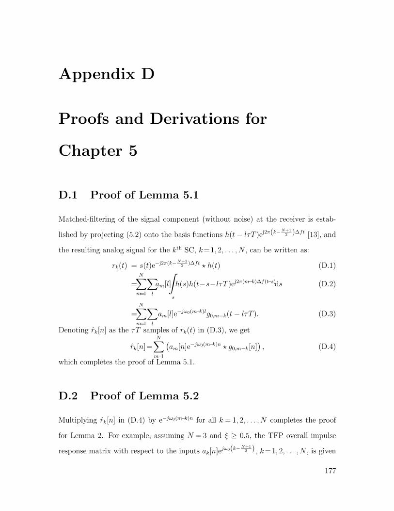
Appendix D


Chapter 5

D.1 Proof of Lemma 5.1

Matched-filtering of the signal component (without noise) at the receiver is estab-

lished by projecting (5.2) onto the basis functions h(t− lτT )ej2π(k−N+12 )∆ft [13], and

the resulting analog signal for the kth SC, k=1, 2, . . . , N , can be written as:

rk(t) = s(t)e−j2π(k−N+12

)∆ft ? h(t) (D.1)

=N∑m=1

∑l

am[l]

∫s

h(s)h(t−s−lτT )ej2π(m−k)∆f(t−s)ds (D.2)

=N∑m=1

∑l

am[l]e−jω0(m−k)lg0,m−k(t− lτT ). (D.3)

Denoting rk[n] as the τT samples of rk(t) in (D.3), we get

rk[n]=N∑m=1

(am[n]e−jω0(m−k)n ? g0,m−k[n]

), (D.4)

which completes the proof of Lemma 5.1.

D.2 Proof of Lemma 5.2

Multiplying rk[n] in (D.4) by e−jω0(m−k)n for all k = 1, 2, . . . , N completes the proof

for Lemma 2. For example, assuming N = 3 and ξ ≥ 0.5, the TFP overall impulse

response matrix with respect to the inputs ak[n]ejω0(k−N+12 ), k=1, 2, . . . , N , is given

177

by:

G[n] =

g−1,−1[n] g0,−1[n] 0

g0,−1[n] g0,0[n] g0,1[n]

0 g0,1[n] g1,1[n]

. (D.5)

178

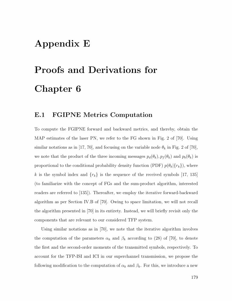
Appendix E


Chapter 6

E.1 FGIPNE Metrics Computation

To compute the FGIPNE forward and backward metrics, and thereby, obtain the

MAP estimates of the laser PN, we refer to the FG shown in Fig. 2 of [70]. Using

similar notations as in [17, 70], and focusing on the variable node θk in Fig. 2 of [70],

we note that the product of the three incoming messages pd(θk), pf (θk) and pb(θk) is

proportional to the conditional probability density function (PDF) p(θk|{rk}), where

k is the symbol index and {rk} is the sequence of the received symbols [17, 135]

(to familiarize with the concept of FGs and the sum-product algorithm, interested

readers are referred to [135]). Thereafter, we employ the iterative forward-backward

algorithm as per Section IV.B of [70]. Owing to space limitation, we will not recall

the algorithm presented in [70] in its entirety. Instead, we will briefly revisit only the

components that are relevant to our considered TFP system.

Using similar notations as in [70], we note that the iterative algorithm involves

the computation of the parameters αk and βk according to (28) of [70], to denote

the first and the second-order moments of the transmitted symbols, respectively. To

account for the TFP-ISI and ICI in our superchannel transmission, we propose the

following modification to the computation of αk and βk. For this, we introduce a new

179

variable

γk = βk −∣∣αk∣∣2 . (E.1)

Moreover, to indicate the polarization labeling and the SC index, we denote these

parameters by α(m)k,x/y, β

(m)k,x/y and γ

(m)k,x/y corresponding to the mth SC and X or Y

polarization, respectively. The modified FGIPNE metrics, stacked as column vectors

with X and Y polarization inputs, are formulated as

[α(m)k,x , α

(m)k,y ]T =

Ls∑j=−Ls

h(m)j,k � E

(a

(m)k−j

)+∑n6=m

Lc∑ν=−Lc

g(n,m)ν,k �E

(a

(n)k−ν

), (E.2)

[γ(m)k,x , γ

(m)k,y ]T =

Ls∑j=−Ls

⟨∣∣h(m)j,k

∣∣⟩2 � Var(a

(m)k−j

)+∑n6=m

Lc∑ν=−Lc

⟨∣∣g(n,m)ν,k

∣∣⟩2�Var(a

(n)k−ν

), (E.3)

where Var(·) and⟨∣∣·∣∣⟩2

denote element-wise variance and absolute-square operations,

respectively. At each LDPC iteration, the expectations and variances in (E.2)-(E.3)

are computed for the constellation symbols using the symbol-probabilities obtained

from the LLRs fed back by the LDPC decoders. Finally, using the statistical property

of the Tikhonov PDF, we obtain the MAP estimate of the PN for the corresponding

polarization and SC as [17]

θMAP = ∠

(2rkα

∗k

2σ2 + γk+ af,k + ab,k

), (E.4)

where ∠(·) denotes the phase angle of a complex scalar, σ2 is the noise variance per

real dimension, and af,k and ab,k are computed according to (36) and (37) of [70],

respectively.

180

Faster-than-Nyquist System Design for Next Generation ...

Documents

Transcript of Faster-than-Nyquist System Design for Next Generation ...