~ Computer Graphics, Volume 21, Number 4, July 1987

Fast Ray Tracing by Ray Classification

James Arvo David Kirk

A p o l l o C o m p u t e r , I n c . 3 3 0 B i l l e r i c a R o a d

C h e l m s f o r d , M A 0 1 8 2 4

A b s t r a c t

We describe a new approach to ray tracing which drastically reduces the number of ray-object and ray-bounds intersection calculations by means of 5-dimensional space subdivision. Collections of rays originating from a common 3D rectangular volume and directed through a 2D solid angle are represented as hypercubes in 5-space. A 5D volume bounding the space of rays is dynamically subdivided into hypercubes, each linked to a set of objects which are candidates for intersection. Rays are classified into unique hypercubes and checked for intersection with the associated candidate object set. We compare several techniques for object extent testing, including boxes, spheres, plane-sets, and convex polyhedra. In addition, we examine optirnizations made possible by the directional nature of the algorithm, such as sorting, caching and backface culling. Results indicate that this algorithm significantly outperforms previous ray tracing techniques, especially for complex environments.

CR Categories and Subject Descriptors: 1.3.3 [Computer Graphics] : Picture/Image Generation; 1.3.7 [Computer Graphics]: Three-Dimensional Graphics and Realism;

General Terms: Algorithms, Graphics

Additional Key Words and Phrases: Computer graphics, ray tracing, visible-surface algorithms, extent, bounding volume, hierarchy, traversal

1. I n t r o d u c t i o n

Our goal in studying algorithms which accelerate ray tracing is to produce high-quality images without paying the enormous time penalty traditionally associated with this method. Recent algorithms have focused on reducing

Permission to copy without foe all or part of this material is granted provided that the copies are not made or distributed for direct commercial advantage, the ACM copyright notice and the title of the publication and its date appear, and notice is given that copying is by permission of the Association for Computing Machinery. To copy otherwise, or to repuNish, requires a fee and/or specific permission.

© 1987 ACM-O-89791-227-6/87/007/0055 $00.75

the number of ray-object intersection tests performed since this is typically where most of the time is spent, especially for complex environments. This is achieved by using a simple-to-evaluate function to cull objects which are clearly not in the path of the ray.

1.1 P r e v i o u s W o r k

Rubin and Whitted [14] developed one of the first schemes for improving ray tracing performance. They observed that "exhaustive search" could be greatly improved upon by checking for intersection with simple bounding volumes around each object before performing more complicated ray-object intersection checks. By creating a hierarchy of bounding volumes, Rubin and Whirred were able to reduce the number of bounding volume intersection checks as well. Weghorst, et. al. [17] studied the use of different types of bounding volumes in a hierarchy, and discussed how ease of intersection testing and "tightness" of fit determine the bounding volume's effectiveness in culling objects.

The object hierarchy of Rubin and Whitted made the crucial step away from the linear time complexity of exhaustive search but still did not achieve acceptable performance on complex environments. This was due in part to the top down search of the object hierarchy required for every ray. Another factor was the difficulty of obtaining a small bound on the number of ray-object intersection tests and ray-bounds comparisons required per ray since this depended strongly on the organization of the hierarchy.

Another class of algorithms employs 3D space subdivision to implement culling functions. The initial candidates for intersection are associated with a 3D volume containing the ray origin. Successive candidates are identified by regions which the ray intersects. Concurrently and independently, Glassner [4], and Fujimoto, et. al. [3] pursued this approach. Glassner investigated partitioning the object space using an octree data structure, while Fujimoto compared octrees to a rectangular linear grid of 3D voxels. Kaplan [7] proposed a similar scheme and observed that a binary space partitioning tree could be used to accomplish the space subdivision. A drawback common to all of these approaches is that a ray which misses everything must be checked against the contents of each of the regions or voxels which it intersects.

55

~ Z ~ SIGGRAPH '87, Anaheim, July 27-31, 1987

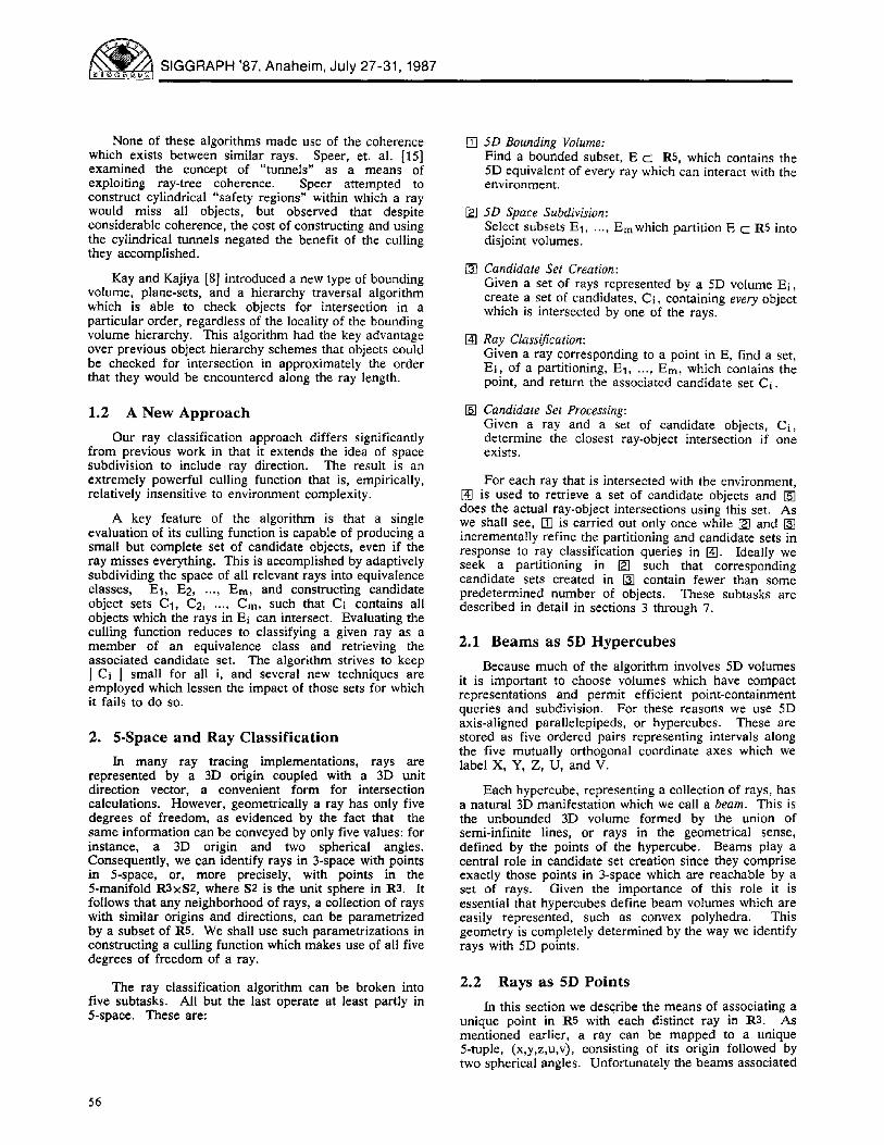
None of these algorithms made use of the coherence which exists between similar rays. Speer, et. al. [15] examined the concept of "tunnels" as a means of exploiting ray-tree coherence. Speer attempted to construct cylindrical "safety regions" within which a ray would miss all objects, but observed that despite considerable coherence, the cost of constructing and using the cylindrical tunnels negated the benefit of the culling they accomplished.

Kay and Kajiya [8] introduced a new type of bounding volume, plane-sets, and a hierarchy traversal algorithm which is able to check objects for intersection in a particular order, regardless of the locality of the bounding volume hierarchy. This algorithm had the key advantage over previous object hierarchy schemes that objects could be checked for intersection in approximately the order that they would be encountered along the ray length.

1 .2 A N e w A p p r o a c h

Our ray classification approach differs significantly from previous work in that it extends the idea of space subdivision to include ray direction. The result is an extremely powerful culling function that is, empirically, relatively insensitive to environment complexity.

A key feature of the algorithm is that a single evaluation of its culling function is capable of producing a small but complete set of candidate objects, even if the ray misses everything. This is accomplished by adaptively subdividing the space of all relevant rays into equivalence classes, El , E2, ..., Era, and constructing candidate object sets C1, C2, ..., Cm, such that Ci contains all objects which the rays in Ei can intersect. Evaluating the culling function reduces to classifying a given ray as a member of an equivalence class and retrieving the associated candidate set. The algorithm strives to keep J Ci I small for all i, and several new techniques are employed which lessen the impact of those sets for which it fails to do so.

2. 5-Space and Ray Classification

In many ray tracing implementations, rays are represented by a 3D origin coupled with a 3D unit direction vector, a convenient form for intersection calculations. However, geometrically a ray has only five degrees of freedom, as evidenced by the fact that the same information can be conveyed by only five values: for instance, a 3D origin and two spherical angles. Consequently, we can identify rays in 3-space with points in 5-space, or, more precisely, with points in the 5-manifold R3xS2, where $2 is the unit sphere in R3. It follows that any neighborhood of rays, a collection of rays with similar origins and directions, can be parametrized by a subset of R5. We shall use such parametrizations in constructing a culling function which makes use of all five degrees of freedom of a ray.

The ray classification algorithm can be broken into five subtasks. All but the last operate at least partly in 5-space. These are:

[ ] 5D Bounding Volume: Find a bounded subset, E c R5, which contains the 5D equivalent of every ray which can interact with the environment.

[]

[]

[]

[ ]

5D Space Subdivision: Select subsets El , ..., Emwhich partition E c R5 into disjoint volumes.

Candidate Set Creation: Given a set of rays represented by a 5D volume Ei , create a set of candidates, Ci , containing every object which is intersected by one of the rays.

Ray Classification: Given a ray corresponding to a point in E, find a set, El , of a partitioning, E1 . . . . , Em, which contains the point, and return the associated candidate set Ci .

Candidate Set Processing: Given a ray and a set of candidate objects, Ci , determine the closest ray-object intersection if one exists.

For each ray that is intersected with the environment, [ ] is used to retrieve a set of candidate objects and [ ] does the actual ray-object intersections using this set. As we shall see, [ ] is carried out only once while [ ] and [ ] incrementally refine the partitioning and candidate sets in response to ray classification queries in [ ] . Ideally we seek a partitioning in [ ] such that corresponding candidate sets created in [ ] contain fewer than some predetermined number of objects. These subtasks are described in detail in sections 3 through 7.

2.1 Beams as 5D Hypercubes

Because much of the algorithm involves 5D volumes it is important to choose volumes which have compact representations and permit efficient point-containment queries and subdivision. For these reasons we use 5D axis-aligned parallelepipeds, or hypercubes. These are stored as five ordered pairs representing intervals along the five mutually orthogonal coordinate axes which we label X, Y, Z, U, and V.

Each hypercube, representing a collection of rays, has a natural 3D manifestation which we call a beam. This is the unbounded 3D volume formed by the union of semi-infinite lines, or rays in the geometrical sense, defined by the points of the hypercube. Beams play a central role in candidate set creation since they comprise exactly those points in 3-space which are reachable by a set of rays. Given the importance of this role it is essential that hypercubes define beam volumes which are easily represented, such as convex polyhedra. This geometry is completely determined by the way we identify rays with 5D points.

2.2 Rays as 5D Points

In this section we describe the means of associating a unique point in R5 with each distinct ray in R3. As mentioned earlier, a ray can be mapped to a unique 5-tuple, (x,y,z,u,v), consisting of its origin followed by two spherical angles. Unfortunately the beams associated

56

(~) ~ Computer Graphics, Volume 21, Number 4, July 1987

with hypercubes under this mapping are not generally polyhedra. To remedy this, we piece together several mappings which have the desired properties locally, and together account for the whole space of rays.

Consider the intersection of a ray with an axis-aligned cube of side two centered at its origin. Each distinct ray direction corresponds to a unique intersection point on this cube. A 2D coordinate system can be imposed on these points by normalizing the ray direction vector, d, with respect to the ¢o-norm, as shown in Equation 1, and extracting (u,v) from the result, as shown

in Equation 2.

d ( dx, dy, d z ) w - - [ 1 1

Ildlloo MAX(Idxl, Idyl, Idzl )

I ( w y , w z ) i f w x = ± 1 , o r e lse

( u , v ) = (Wx, W z ) i f w y = :t:1, o r e lse [2]

( W , W y ) i f W z = ::t:1

This establishes a one-to-one correspondence between [ -1 ,1Ix[ -1 ,1] and rays passing through a single face of the cube. By partitioning the rays into six dominant directions defined by the faces of the cube, and restricting the mapping to each of these domains, we obtain six bicontinuous one-to-one mappings. We associate each with a dominant axis, denoted +X, -X, +Y, -Y, +Z, or -Z . The inverse mappings, or parametrizations, define an atlas of $2, covering the set of ray directions with images of [ -1 ,1]x[ -1 ,1] . This is trivially extended to R3xS2. In order to meet our requirement of a global one-to-one correspondence, however, we index into six "copies" of [ -1 ,1]x[-1 ,1] using the dominant axis of a ray. For a given ray, this axis is determined by the axis and sign of its largest absolute direction component.

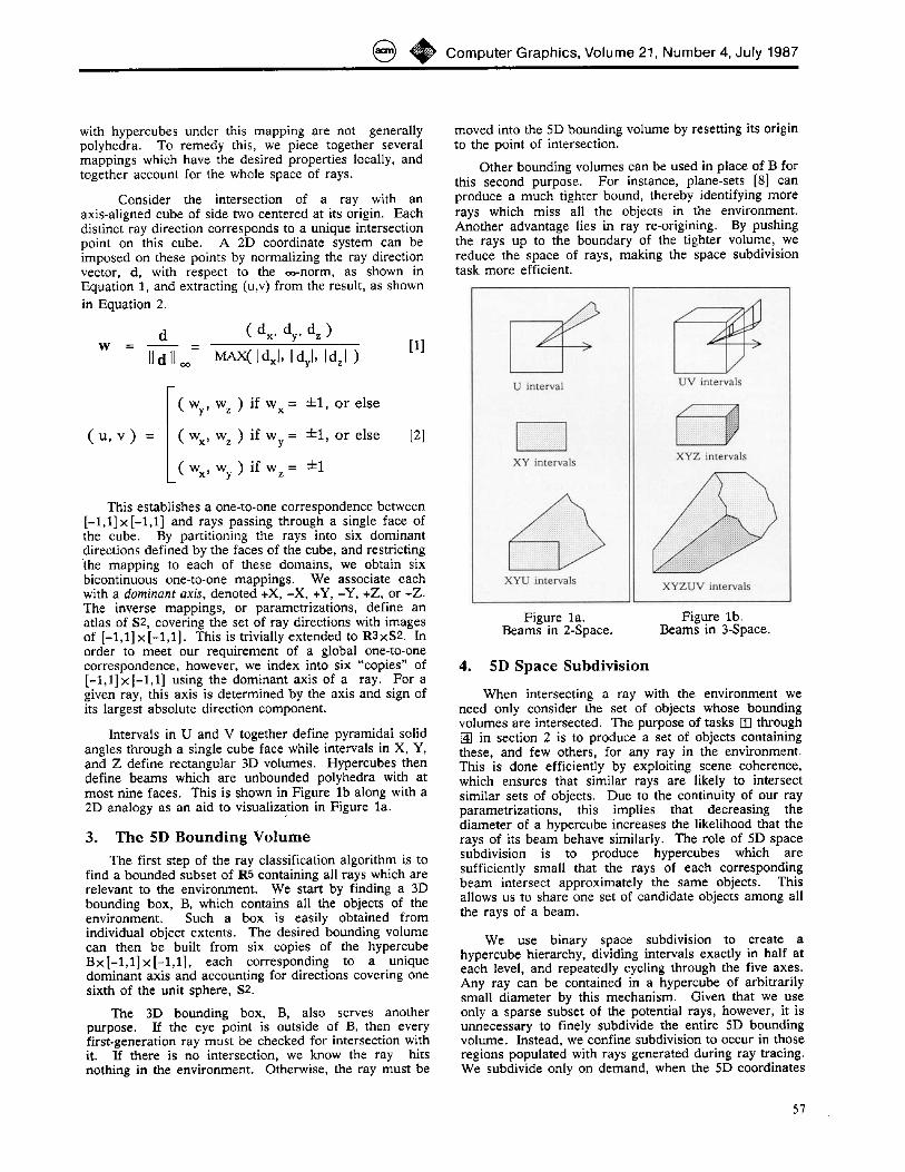
Intervals in U and V together define pyramidal solid angles through a single cube face while intervals in X, Y, and Z define rectangular 3D volumes. Hypercubes then define beams which are unbounded polyhedra with at most nine faces. This is shown in Figure l b along with a 2D analogy as an aid to visualization in Figure la .

3. T h e 5D B o u n d i n g V o l u m e

The first step of the ray classification algorithm is to find a bounded subset of R5 containing all rays which are relevant to the environment. We start by finding a 3D bounding box, B, which contains all the objects of the environment. Such a box is easily obtained from individual object extents. The desired bounding volume can then be built from six copies of the hypercube Bx[ -1 ,1 ]× [ -1 ,1 ] , each corresponding to a unique dominant axis and accounting for directions covering one sixth of the unit sphere, S2.

The 3D bounding box, B, also serves another purpose. If the eye point is outside of B, then every first-generation ray must be checked for intersection with it. If there is no intersection, we know the ray hits nothing in the environment. Otherwise, the ray must be

moved into the 5D bounding volume by resetting its origin to the point of intersection.

Other bounding volumes can be used in place of B for this second purpose. For instance, plane-sets [8] can produce a much tighter bound, thereby identifying more rays which miss all the objects in the environment. Another advantage lies in ray re-origining. By pushing the rays up to the boundary of the tighter volume, we reduce the space of rays, making the space subdivision task more efficient.

U interval

XY intervals

XYU intervals

UV intervals

XYZ intervals

x Y z u v intervals

Figure la . Beams in 2-Space.

Figure lb . Beams in 3-Space.

4. 5D Space Subdivision

When intersecting a ray with the environment we need only consider the set of objects whose bounding volumes are intersected. The purpose of tasks [ ] through [ ] in section 2 is to produce a set of objects containing these, and few others, for any ray in the environment. This is done efficiently by exploiting scene coherence, which ensures that similar rays are likely to intersect similar sets of objects. Due to the continuity of our ray parametrizations, this implies that decreasing the diameter of a hypercube increases the likelihood that the rays of its beam behave similarly. The role of 5D space subdivision is to produce hypercubes which are sufficiently small that the rays of each corresponding beam intersect approximately the same objects. This allows us to share one set of candidate objects among all the rays of a beam.

We use binary space subdivision to create a hypercube hierarchy, dividing intervals exactly in half at each level, and repeatedly cycling through the five axes. Any ray can be contained in a hypercube of arbitrarily small diameter by this mechanism. Given that we use only a sparse subset of the potential rays, however, it is unnecessary to finely subdivide the entire 5D bounding volume. Instead, we confine subdivision to occur in those regions populated with rays generated during ray tracing. We subdivide only on demand, when the 5D coordinates

57

~ SIGGRAPH '87, Anaheim, July 27-31, 1987

of a ray are found to reside in a hypercube which is too large. Thus, beginning with the six bounding hypercubes, we construct the entire hierarchy by lazy evaluation.

When a ray causes new paths to be formed in the hypercube hierarchy, two heuristics determine when subdivision terminates. We stop if either the candidate set or the hypercube falls below a fixed size threshold. A small candidate set indicates that we have achieved the goal of making the associated rays inexpensive to intersect with the environment. The hypercube size constraint is imposed to allow the cost of creating a candidate set to be amortized over many rays.

5. Candidate Set Creation

Given a hypercube, the task of creating its candidate set consists of determining all the objects in the environment which its rays can intersect. This is done by comparing each object 's bounding volume with the beam defined by the hypercube. If the volumes intersect, the object is classified as a candidate with respect to that hypercube and is added to the candidate set.

The six bounding hypercubes are assigned candidate sets containing all objects in the environment. As subdivision proceeds, candidate sets are efficiently created for the new hypercubes by making use of the hierarchy. Only those objects in an ancestor 's candidate set need be reclassified.

For space efficiency, we need not create a candidate set for every intermediate hypercube in the hierarchy. When a hypercube is subdivided along one axis, the beams of the resulting hypercubes usually overlap substantially, and are quite similar to the parent beam. Consequently, a single subdivision eliminates few candidates. This suggests performing several subdivisions before creating a new candidate set. A strategy which we have found to be effective is to subdivide each of the five axes before creating a new candidate set. While this allows up to 2 s hypercubes to derive their candidate sets from the same ancestor, the reduction in storage is significant. Also, due to lazy evaluation of the hierarchy, it is rare that all descendants are even created.

5.1 Object Class i f icat ion

The object classification method used in candidate set creation is critical to the performance of the ray tracer. A very fast method may be too conservative, creating candidate sets which are much too large. This causes unnecessary overhead in both candidate set creation and processing. A classifying method which performs well in rejecting objects may be unacceptable if it is too costly. As with object extents used for avoiding unnecessary ray-object intersection checks, there must be a compromise between the cost of the method and its accuracy [17]. In the following subsections we discuss the tradeoffs of three object classification techniques which can be used independently or in combination.

5.1.1 Classifying Objects with LP

The first object classification method we describe employs linear programming to test for object-beam intersection, and requires objects to be enclosed by convex polyhedra. A polyhedral bounding volume is conveniently represented by its vertex list, or hull points, and can be made arbitrarily close to the convex hull of the object. Since the beam is itself a polyhedron, the object classification problem reduces to test ing for intersection between two polyhedra. This is easily expressed as a linear program using the hull points [12] and then solved using the simplex method [13]. The result is an exact classification scheme for this type of bounding volume. That is, an object is classified as a candidate of a hypercube if and only if some ray of the beam intersects its bounding polyhedron.

Unfortunately, our experience has shown that the computation required to solve the linear program is prohibitively high, precluding its use as the primary object classification method. It is overly complex for handling the very frequent cases of objects which are either far from the beam or inside it. Nevertheless, it is a useful tool for testing and evaluating the effectiveness of approximate object-classification methods.

5.1.2 Classifying Objects with Planes

The linear programming approach rejects an object from the candidate set if and only if there exists a separating plane between the beam and the object 's bounding polyhedron. This suggests a simpler approach which tests several planes directly, classifying an object as a candidate if none of the planes are separators.

For every beam there are several planes which are particularly appropriate to test, each with the entire beam in its positive half-space. Four of these planes are parallel to the faces of the UV pyramid, translated to the appropriate XYZ extrema of the hypercube. Up to three more are found "behind" the beam, containing faces of the XYZ hypercube extent. If all of the vertices of an object 's bounding polyhedron are found to be in the negative half-space of one of these planes, the object is rejected. The half-space tests are greatly simplified by the nature of these planes, since all are parallel to at least one coordinate axis.

This method is fast and conservative, never rejecting an object which is actually intersected by the beam. It is

also approximate, since objects will be erroneously classified as candidates when, for example, their bounding polyhedra intersect both a U and a V plane without intersecting the beam.

5.1.3 Classifying Objects wi th Cones

Another approach to object classification uses spheres to bound objects and cones to approximate beams. This is similar to previous uses of cones in ray tracing. Amanatides [1] described the use of cones as a method of area sampling, providing accurate and inexpensive anti-aliasing. Kirk [9] used cones as a tool to calculate proper texture filtering apertures, and to improve anti-aliasing of bump-mapped surfaces. In our context, cones prove to be very effective for classifying objects bounded by spherical extents.

58

( ~ ~ Computer Graphics, Volume 21, Number 4, July 1987

TO create a candidate set for a hypercube we begin by constructing a cone, specified by a unit axis vector, W, a spread angle, 0, and an apex, P, which completely contains the beam of the hypercube. If this cone does not intersect the spherical extent of an object, the object is omitted from the candidate set. The details of the cone-sphere intersection calculation are given in both [1] and [9]. We describe the construction of the cone below with the aid of function F in Equation 3, which defines inverse mappings of those described in section 2.2.

F ( u , V) =

( 1, u, v ) if +Xis dominant

( - 1 , u, v ) if - X i s dominant

( u, 1, v ) if +Y is dominant

( u , - 1 , v ) if - Y i s dominant

( u, v, 1 ) if +Z is dominant

( u, v , - 1 ) if - Z i s dominant

131

The cone axis vector, W, depends only on the dominant axis of the hypercube and its U and V intervals, (umin,umax) and (vmin, vmax). It is constructed by bisecting the angle between the vectors A and B, which are given by Equations 4 and 5.

A -- F( umin, vmax ) [4]

B = F( umax, vmin ) [5] To find the cone spread angle we also construct

vectors C and D using Equations 6 and 7. We then compute 0 as shown in Equation 8.

C = F( umin, vmin ) [6]

D -- F( umax, vmax ) [7]

0 = ~¢[AX( A/W, B/W, CgW, D / W ) [8]

Once the axis and spread angle are known, the apex of the cone, P, is determined by the 3D rectangular volume, R, defined by the XYZ intervals of the hypercube. The point P is located by displacing the centroid of R in the negative cone axis direction until the cone exactly contains the smallest sphere bounding R. The resulting expression for P is given in Equation 9, where R0 and R1 are the min and max extrema of R.

1% + R1 II R 0 - R1 IIz P - W [9] 2 2 SINe

The cone is used to classify all potential candidates of the hypercube and is constructed only once per hypercube. The comparison between the cone and the object's bounding sphere is fast, making the cost of a distant miss low. This reduces the penalty of infrequent candidate list creation, the space saving measure discussed in section 5.

A linear transformation, M, applied to an object can also be used to modify its bounding sphere. By

transforming the center of the sphere by M and scaling its radius by II M 112, we obtain a new sphere which is guaranteed to contain the transformed object. The matrix 2-norm is given by x/( P( M 7M ) ) [11], where 0, the spectral radius, is the largest absolute eigenvalue of a matrix. If MTM is sparse, the eigenvalue calculation is quite simple. An iterative technique like the power method can be used for the remaining cases [5].

6. Ray Class i f icat ion

Every ray-environment intersection calculation begins with ray classification, which locates the hypercube containing the 5D equivalent of the ray. This entails mapping the ray into a 5D point and traversing the hypercube hierarchy, beginning with the bounding hypereube indexed by the dominant axis of the ray, until we reach the leaf containing this point. Due to lazy evaluation of the hierarchy, this traversal may have the side effect of creating a new path terminating at a sufficiently small hypercube containing the ray if such a path has not already been built on behalf of another ray. If the candidate set associated with the leaf hypercube is empty, we are guaranteed that the ray intersects nothing. Otherwise, we process this set as described in the next section.

7. Candidate Set Processing

Once ray classification has produced a set of candidate objects for a given ray, this set must be processed to determine the object which results in the closest intersection, if one exists. To optimize this search we continue to make use of object bounding volumes for coarse intersection checks. We also reject objects whose bounding volumes intersect the ray beyond a known object intersection. This can further reduce the number of ray-object intersection calculations, but still requires that the ray be tested against all bounding volumes of the candidate set.

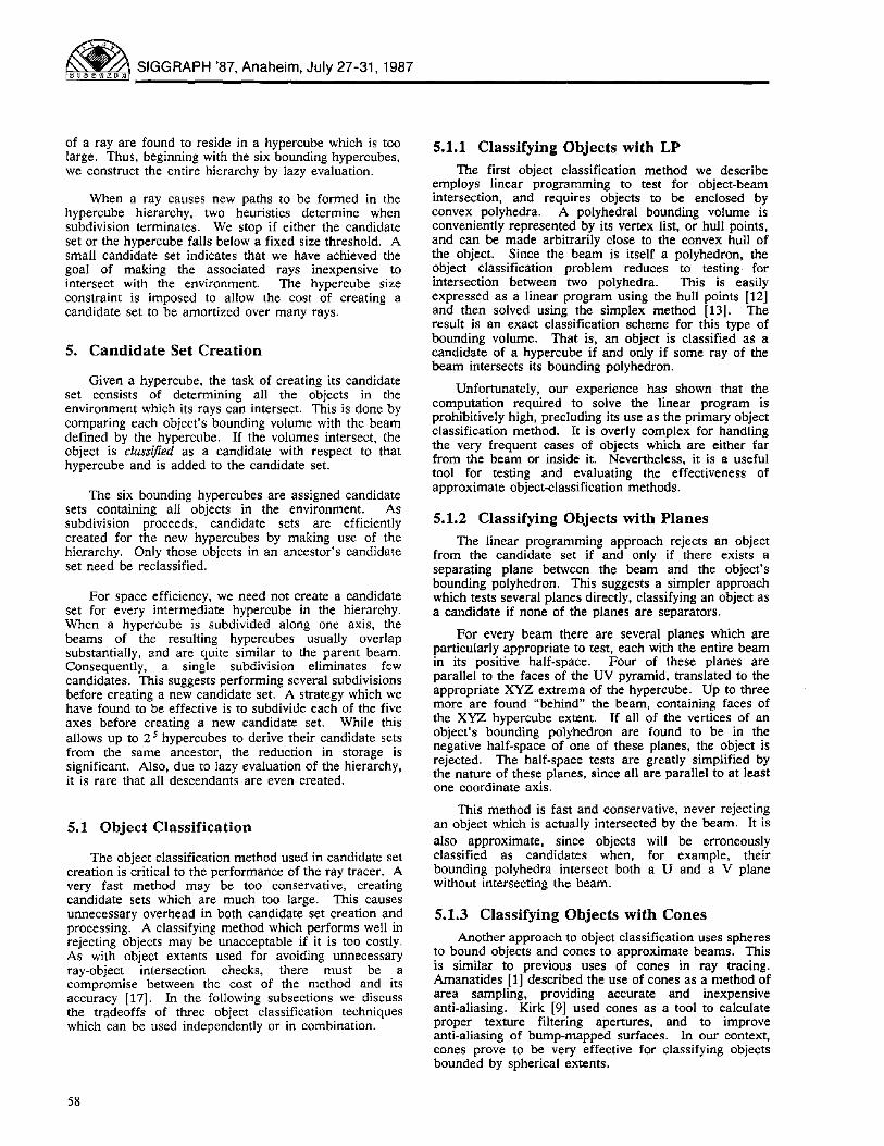
We can remove this latter requirement by taking advantage of the fact that all rays of a given beam share the same dominant axis. By sorting the objects of the candidate sets by their minimum extents along this axis, then processing them in ascending order, we can ignore the tail of the list if we reach a candidate whose entire extent lies beyond a known intersection. This is an enormous advantage because it can drastically reduce the number of bounding volume checks in cases where the ray intersects an object near the head of the list. For example, in Figure 2 only the first two objects are tested because all subsequent objects are guaranteed to lie beyond the known intersection. By sorting the candidate sets of the six bounding hypercubes along the associated dominant axes before 5D space subdivision begins, the correct ordering can be inherited by all subsequent candidate sets with no additional overhead. Object bounding boxes provide the six keys used in sorting these initial candidate sets.

59

~ SIGGRAPH '87, Anaheim, July 27-31 1987

I 1

Figure 2.

:::.- ::ibeam i

[ I dominant axis 3 4 5

Sorted candidates.

8. B a c k f a c e C u l l i n g

Though backface culling is a popular technique in the field of computer graphics [10], it has previously been of very limited use in ray tracing since polygons which are not in the direct line of sight can still affect the environment by means of shadows, reflections, and transparency. When creating the candidate set of a hypercube, however, it is appropriate to eliminate those polygons which are part of an opaque solid and are backfacing with respect to every ray of its beam. When classifying with cones, this latter criterion is met if Equation 10 is satisfied, where N is the front-facing normal of the polygon, W is the cone axis, and 0 is the cone spread angle.

N . w > SIN 0 [10]

Using this technique, rays headed in opposite directions through the same volume of space may be tested against totally disjoint sets of polygons. By eliminating nearly half the candidates of most hypercubes, backface culling greatly accelerates both the creation and processing of candidate sets.

9. I m a g e C o h e r e n c e a n d C a c h i n g

Due to image coherence, two neighboring samples in image space will tend to produce very similar ray trees. This implies that successive rays of a given generation will tend to be elements of the same beam. We use this fact to great advantage by caching the most recently referenced hypercubes of each generation and checking new rays first against this cache. If a ray is contained, it is a cache hit, and the previous candidate set is returned immediately, without re-traversing the hypercube hierarchy. Otherwise, we classify the ray by traversal and update the cache with the new hypercube and candidate set. Although hierarchy traversal is very efficient, verifying that a point lies within a hypercube requires only ten comparisons, a considerable shortcut.

A related caching technique is used exclusively for shadows. Rays used for sampling light sources are special because there is no need to compute the closest intersection. It suffices to determine the existence of an opaque object between the ray origin and the intersection with the light source. If a given point in 3-space is in shadow, nearby points are likely shadowed by the same object. The shadow cache simply records the last object casting a shadow with respect to each light source and checks that object first, as part of the next shadow calculation.

10. C a n d i d a t e Set T r u n c a t i o n

Because we cannot decide when one object occludes another based on bounding volumes alone, a candidate set must contain all objects whose bounding volumes intersect the beam. Thus, even extremely narrow beams can produce candidate sets which are large. This poses no problem for candidate set processing because sorting insures that far-away occluded objects will never be tested. This does increase storage requirements, however, by increasing the number of candidate sets which contain a given object.

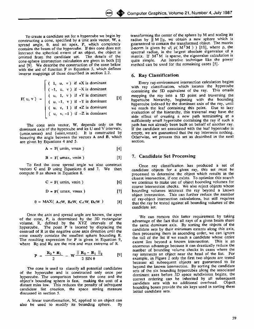
We can drop far-away objects from a candidate set at the expense of a slight penalty incurred by rays which are not blocked by the nearer objects. This is done by truncating a sorted candidate set at a point where the remaining objects are outside the XYZ extent of the hypercube and marking this point with a truncation plane orthogonal to the dominant axis. For example, in Figure 2 this could occur just before the fourth object. We process a truncated candidate set differently only when no object intersection is found in front of the truncation plane. See Figure 3. In this case we re-position the ray to the truncation plane, re-classify, and process the new candidate set. Though this is similar to previous 3D space subdivision techniques [3][4][7], we retain the distinct advantages of sorting and backface culling within the truncated candidate sets, as well as the ability to pass rays through unobstructed regions of space with virtually no work.

We reduce the cost of occasional re-classification steps by adding a cache dimension indicating the number of times a ray has been reclassified. This allows most re-classifications to be done without traversing the hypercube hierarchy. Moreover, re-reclassifying a ray often results in a net gain by narrowing the included volume as we proceed further away from the original ray origin. See Figure 4.

Figure 3. Set truncation.

Figure 4. Beam narrowing.

11. F i r s t - G e n e r a t i o n Rays

First-generation rays have only two degrees of freedom, making them easy to characterize, and frequently outnumber all other rays, making them important to optimize. Many ray tracing implementations obviate the need for first-generation rays altogether by means of more conventional scan-line or depth-buffer algorithms. For extremely complex environments, however, the value of these methods diminishes, since they are forced to expend some effort on every object, even those which do not contribute to the final image. It is therefore worthwhile to examine ray tracing techniques which can perform superlinearly on these rays.

60

( ~ ~ Computer Graphics, Volume 21, Number 4, July 1987

The ray classification algorithm benefits in a number of ways from the special nature of first-generation rays. Because they originate from a degenerate 3D volume, the eye point, first-generation rays can be classified using u and v alone. This increases the efficiency of ray classification by simplifying the traversal of the hypercube hierarchy, which becomes a hierarchy of 2D rectangles. Candidate set creation also benefits because the beams associated with the degenerate hypercubes are non- overlapping pyramids. Candidate sets are therefore cut in half, on average, with every subdivision. This makes it feasible to obtain smaller candidate sets, thereby speeding up candidate set processing as well. The result of these optimizations for first-generation rays is an image-space algorithm which closely resembles the 2D recursive subdivision approach introduced by Warnock [16].

12. S u m m a r y

We have described a method which accelerates ray tracing by drastically reducing the number of ray-object and ray-bounds intersection checks. This is accomplished by extending the notion of space subdivision to a 5D scheme which makes use of ray direction as well as ray origin. Rays are classified into 5D hypercubes in order to retrieve pre-sorted sets of candidate objects which are efficiently tested for intersection with each ray. The computational cost of intersecting a ray with the environment is very low because similar rays share the benefit of culling far-away objects, thereby exploiting coherence. This technique can be used to accelerate all applications which rely upon ray-environment inter- sections, including those which perform Monte Carlo integration [2][6]. Empirical evidence indicates that performance is closer to constant time than previous methods, especially for very complex environments.

13. R e s u l t s

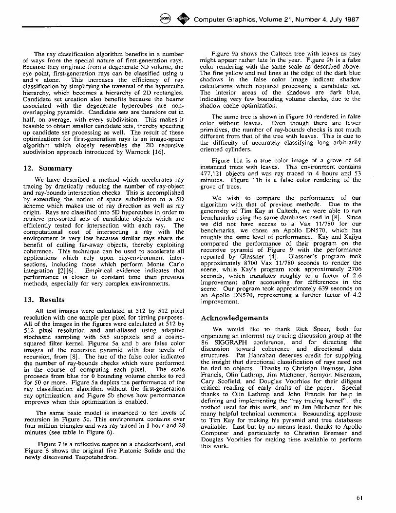
All test images were calculated at 512 by 512 pixel resolution with one sample per pixel for timing purposes. All of the images in the figures were calculated at 512 by 512 pixel resolution and anti-aliased using adaptive stochastic sampling with 5x5 subpixels and a cosine- squared filter kernel. Figures 5a and b are false color images of the recursive pyramid with four levels of recursion, from [8]. The hue of the false color indicates the number of ray-bounds checks which were performed in the course of computing each pixel. The scale proceeds from blue for 0 bounding volume checks to red for 50 or more. Figure 5a depicts the performance of the ray classification algorithm without the first-generation ray optimization, and Figure 5b shows how performance improves when this optimization is enabled.

The same basic model is instanced to ten levels of recursion in Figure 5c. This environment contains over four million triangles and was ray traced in 1 hour and 28 minutes (see table in Figure 6).

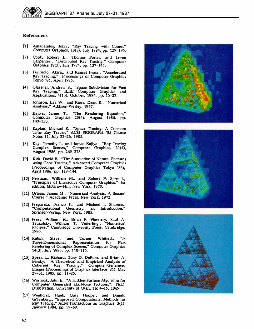
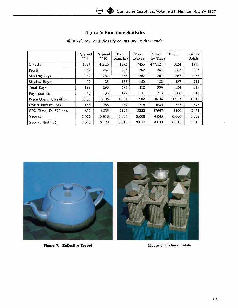
Figure 7 is a reflective teapot on a checkerboard, and Figure 8 shows the original five Platonic Solids and the newly discovered Teapotahedron.

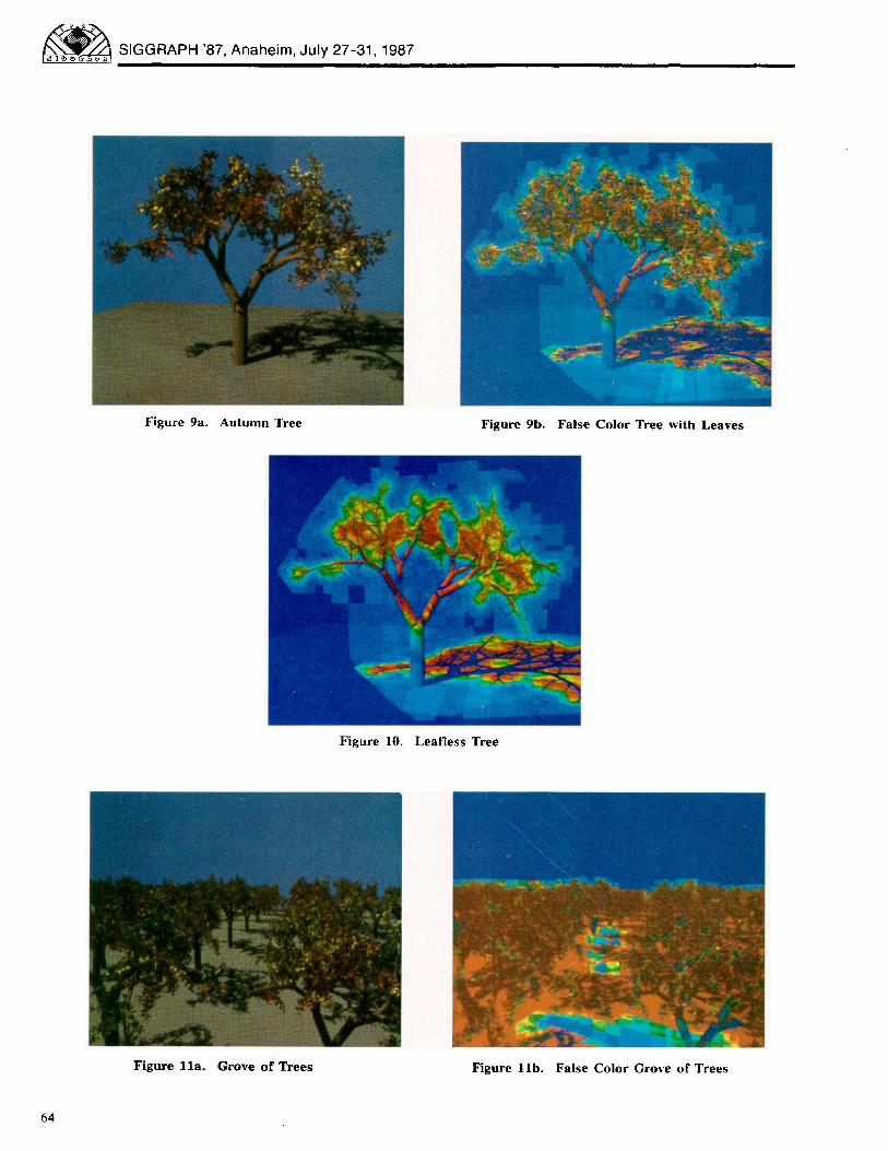
Figure 9a shows the Caltech tree with leaves as they might appear rather late in the year. Figure 9b is a false color rendering with the same scale as described above. The fine yellow and red lines at the edge of the dark blue shadows in the false color image indicate shadow calculations which required processing a candidate set. The interior areas of the shadows are dark blue, indicating very few bounding volume checks, due to the shadow cache optimization.

The same tree is shown in Figure 10 rendered in false color without leaves. Even though there are fewer primitives, the number of ray-bounds checks is not much different from that of the tree with leaves. This is due to the difficulty of accurately classifying long arbitrarily oriented cylinders.

Figure 11a is a true color image of a grove of 64 instanced trees with leaves. This environment contains 477,121 objects and was ray traced in 4 hours and 53 minutes. Figure 11b is a false color rendering of the grove of trees.

We wish to compare the performance of our algorithm with that of previous methods. Due to the generosity of Tim Kay at Caltech, we were able to run benchmarks using the same databases used in [8]. Since we did not have access to a Vax 11/780 for our benchmarks, we chose an Apollo DN570, which has roughly the same level of performance. Kay and Kajiya compared the performance of their program on the recursive pyramid of Figure 9 with the performance reported by Glassner [4]. Glassner's program took approximately 8700 Vax 11/780 seconds to render the scene, while Kay's program took approximately 2706 seconds, which translates roughly to a factor of 2.6 improvement after accounting for differences in the scene. Our program took approximately 639 seconds on an Apollo DN570, representing a further factor of 4.2 improvement.

A c k n o w l e d g e m e n t s

We would like to thank Rick Speer, both for organizing an informal ray tracing discussion group at the 86 SIGGRAPH conference, and for directing' the discussion toward coherence and directional data structures. Pat Hanrahan deserves credit for supplying the insight that directional classification of rays need not be tied to objects. Thanks to Christian Bremser, John Francis, Olin Lathrop, Jim Michener, Semyon Nisenzon, Cary Scofield, and Douglas Voorhies for their diligent critical reading of early drafts of the paper. Special thanks to Olin Lathrop and John Francis for help in defining and implementing the "ray tracing kernel", the testbed used for this work, and to Jim Michener for his many helpful technical comments. Resounding applause to Tim Kay for making his pyramid and tree databases available. Last but by no means least, thanks to Apollo Computer and particularly to Christian Bremser and Douglas Voorhies for making time available to perform this work.

61

~ SIGGRAPH '87, Anaheim, July 27-31, 1987

References

[1] Amanatides, John., "Ray Tracing with Cones," Computer Graphics, 18(3), July 1984, pp. 129-135.

[2] Cook, Robert L., Thomas Porter, and Loren Carpenter., "Distributed Ray Tracing," Computer Graphics 18(3), July 1984, pp. 137-145.

[3] Fujimoto, Akira,, and Kansei Iwata., "Accelerated Ray Tracing," Proceedings of Computer Graphics Tokyo '85, April 1985.

[4] Glassner, Andrew S., "Space Subdivision for Fast Ray Tracing," IEEE Computer Graphics and Applications, 4(10), October, 1984, pp. 15-22.

[5] Johnson, Lee W., and Riess, Dean R., "Numerical Analysis," Addison-Wesley, 1977.

[6] Kajiya, James T., "The Rendering Equation," Computer Graphics 20(4), August 1986, pp. 143-150.

[7] Kaplan, Michael R., "Space Tracing: A Constant Time Ray Tracer," ACM SIGGRAPH '85 Course Notes 11, July 22-26, 1985.

[8] Kay, Timothy L. and James Kajiya., "Ray Tracing Complex Scenes," Computer Graphics, 20(4), August 1986, pp. 269-278.

[9] Kirk, David B., "The Simulation of Natural Features using Cone Tracing," Advanced Computer Graphics (Proceedings of Computer Graphics Tokyo '86), April 1986, pp. 129-144.

[10] Newman, William M., and Robert F. Sproull., "Principles of Interactive Computer Graphics," 1st edition, McGraw-Hill, New York, 1973.

[11] Ortega, James M., "Numerical Analysis, A Second Course," Academic Press, New York, 1972.

[12] Preparata, Franco P., and Michael I. Shamos., "Computational Geometry, an Introduction," Springer-Verlag, New York, 1985.

[13] Press, William H., Brian P..Flannery, Saul A. Teukolsky, William T. Vetterling., "Numerical Recipes," Cambridge University Press, Cambridge, 1986.

[14] Rubin, Steve, and Turner Whitted., "A Three-Dimensional Representation for Fast Rendering of Complex Scenes," Computer Graphics 14(3), July 1980, pp. 110-116.

[15] Speer, L. Richard, Tony D. DeRose, and Brian A. Barsky., "A Theoretical and Empirical Analysis of Coherent Ray Tracing," Computer-Generated Images (Proceedings of Graphics Interface '85), May 27-31, 1985, pp. 11-25.

[16] Warnock, John E., "A Hidden-Surface Algorithm for Computer Generated Half-tone Pictures,", Ph.D. Dissertation, University of Utah, TR 4-15, 1969.

[17] Weghorst, Hank, Gary Hooper, and Donald Greenberg., "Improved Computational Methods for Ray Tracing," ACM Transactions on Graphics, 3(1), January 1984, po. 52-69.

62

( ~ ~ Computer Graphics, Volume 21, Number 4, July 1987

Figure 6: R u n - t i m e Statist ics

All pixel, ray, and classify counts are in thousands

Pyramid Pyramid Tree Tree Grove Teapot Platonic * '4 ** I0 Branches Leaves 64 Trees Solids

Objects 1024 4.2E6 1272 7455 477,121 1824 1405

Pixels 262 262 262 262 262 262 262

Shading Rays 262 262 262 262 262 262 262

37 28 133 150 128 187 224 Shadow Rays

Total Rays 299 290 395 412 390 534 515

Rays that hit 43 30 149 191 213 206 240

Beam/Object Classifies 10.50 117.06 16.01 17.02 46.46 47.71 10.41

Object Intersections 188 288 989 716 1884 523 4896

CPU Time, DN570 sec. 639 5335 2194 3230 17607 3100 2474

(sec/ray) 0.002 0.018 0.006 0.008 0.045 0.006 0.008

(sec/ray that hit) 0.015 0.178 0.015 0.017 0.083 0.015 0.010

Figure 7. Reflective Teapot

!i! I~

Figure 8. Platonic Solids

63

• SIGGRAPH '87, Anaheim, July 27-31 1987

I ~ ~ ® ~ [ IH[I

F igure 9a. Au tumn Tree Figure 9b. Fa l se Color Tree with Leaves

Figure 10. Leaf less Tree

F igure 11a. Grove o f Trees Figure l i b . Fa lse Color Grove of Trees

64