Fast Parallel Surface and Solid Voxelization on GPUs

Michael Schwarz∗ Hans-Peter Seidel

Max-Planck-Institut Informatik

Conservative

Rasterization

Conservative

voxelization

Voxelization via

rasterization

(from 3 directions)

Octree-based sparse solid voxelization

Figure 1: Our methods can rapidly create surface and solid voxelizations, surpassing the limitations of rasterization-based approaches. Left:The conservative voxelization robustly captures all overlapped voxels. Right: Exploiting the uniformity of large voxel regions, we can directlyperform solid voxelization into a sparse octree, significantly reducing the memory requirements.

Abstract

This paper presents data-parallel algorithms for surface and solidvoxelization on graphics hardware. First, a novel conservativesurface voxelization technique, setting all voxels overlapped by amesh’s triangles, is introduced, which is up to one order of magni-tude faster than previous solutions leveraging the standard rasteri-zation pipeline. We then show how the involved new triangle/boxoverlap test can be adapted to yield a 6-separating surface voxeliza-tion, which is thinner but still connected and gap-free. Comple-menting these algorithms, both a triangle-parallel and a tile-basedtechnique for solid voxelization are subsequently presented. Fi-nally, addressing the high memory consumption of high-resolutionvoxel grids, we introduce a novel octree-based sparse solid vox-elization approach, where only close to the solid’s boundary finest-level voxels are stored, whereas uniform interior and exterior re-gions are represented by coarser-level voxels. This representationis created directly from a mesh without requiring a full intermediatesolid voxelization, enabling GPU-based voxelizations of unprece-dented size.

Keywords: voxelization, GPU computing, overlap testing, paralleldata structure creation, octree

1 Introduction

Binary voxel representations are heavily employed in computergraphics. They are typically derived as discrete approximations ofobjects via a process called voxelization. In a surface voxelization,all voxels are set that fulfill some overlap or distance criterion withrespect to a surface, whereas a solid voxelization sets all voxels con-sidered interior to an object.

∗e-mail: mschwarz@mpi-inf.mpg.de

Offering a regular representation that is independent from objectand surface complexity, voxelizations are used in domains as di-verse as 3D shape matching and visibility processing. In the lat-ter, for instance, rays may be cast against a dynamically createdscene voxelization to determine occlusion when computing light-ing [Nichols et al. 2010] or ambient occlusion [Reinbothe et al.2009]. Another application is collision detection, where a voxel-wise comparison of the voxelizations of two objects easily identifiescollisions. Similarly, bitwise combinations of solid voxelizationsare naturally applicable for performing constructive solid geometrytasks. Voxelizations are also helpful for establishing computationaldomains, e.g. for fluid simulations with obstacles or for light prop-agation.

Since voxelization is often a performance-critical, integral part, sev-eral algorithms have been proposed to perform voxelization of tri-angle meshes on the GPU, leveraging the fast rasterization pipelinefor this 3D scan conversion. However, this inviting use of the ras-terizer causes most surface voxelization approaches to suffer fromgaps and missed thin features in the voxelization, mainly because avoxel is only set if the triangle overlaps the corresponding pixel’scenter. Although this can be alleviated by manually enlarging thetriangle’s pixel footprint in the geometry shader stage, resulting al-gorithms are typically rather slow, hampering their utility for real-time applications. Concerning solid voxelization, a fast, straight-forward approach exists [Eisemann and Decoret 2008] but unfor-tunately only works with OpenGL, as it relies on bitwise blendingoperations, which are no longer exposed in Direct3D. By contrast,alternative solutions processing voxel slices sequentially are gener-ally supported by all graphics APIs but are much slower.

In this paper, we approach voxelization with new data-parallel al-gorithms that utilize GPUs as general, massively parallel computedevices instead of building on the standard pipeline. Basically, theyreplace the fixed-function 2D rasterizer by a collection of custom“3D rasterizers”. This has several advantages. First, we don’t haveto indirectly modify the rasterizer’s pixel coverage test by appro-priately enlarging input triangles and discarding superfluous frag-ments, which constitutes extra work and occupies processing units,but can directly apply our desired coverage criterion. Second, wemay dynamically choose the coordinate plane (xy, xz or yz) opti-mal for processing on a per-triangle basis, whereas in the standardpipeline this involves a separate rendering for each coordinate planeas well as a subsequent data merging step. This is due to the texture-based encoding of the voxelization, e.g. across multiple channels of

a texture array. By contrast, we are free to adopt any storage orga-nization scheme and can access this arbitrarily.

In particular, this freedom enables us to account for the fact that sur-face voxelizations are typically populated rather sparsely and that,analogously, solid voxelizations usually encompass many uniformregions. For instance, we could store such a voxelization in a sparseoctree, where a coarser-level node is only refined if the representedvoxel space is non-uniform, i.e. finest-level nodes merely exist forvoxels close to the object’s boundary. As we show in this paper,such a space-efficient voxelization representation can be created di-rectly from an input mesh without having to first derive an interme-diate full voxelization. Hence, it becomes easily possible to copewith voxelizations of grid size 40963, which would require 8 GBof memory if represented fully as bit array. As an additional ben-efit, the hierarchical representation enables faster processing of thevoxel data, e.g. during ray traversal.

This paper covers a wide spectrum of voxelization procedures withdedicated data-parallel solutions that take the above considerationsinto account. Initially, we focus on surface voxelization (Sec. 3) andpresent a new parallel algorithm for fast conservative voxelization,where all voxels overlapped by a triangle are identified and set, uti-lizing a new triangle/box overlap test. Adapting this test, we thenaddress creating a thinner, 6-separating voxelization. Subsequently,we turn to solid voxelization (Sec. 4) and introduce both a direct,triangle-parallel approach and an advanced tile-based algorithm.Finally, we present a novel octree-based sparse solid voxelizationtechnique (Sec. 5), demonstrating the direct scan-conversion of tri-angles into a sparse spatial data structure on the GPU.

Numerous applications that utilize voxelizations can directly profitfrom our methods. Generally, they enable speeding up these appli-cations, improving their attainable quality (e.g. because conserva-tive voxelization becomes affordable in real-time scenarios), or us-ing larger voxelizations without negatively affecting memory con-sumption or construction time.

2 Related work

Real-time voxelization Many voxelization algorithms with var-ious properties have been devised. Among the most relevant real-time approaches, Fang and Chen [2000] construct a surface vox-elization slice-wise, rendering the geometry once for each voxelslice while restricting the view volume to this slice. To reduce thenumber of rendering passes, Li et al. [2005] employ depth peelingto capture all surface points and then scatter them into a flattenedvoxel grid via point rendering. The peeling process is done along allthree orthogonal voxel grid axes to decrease the number of missedvoxels. While these approaches spend one texel for storing a voxel,Dong et al. [2004] encode binary voxels in separate bits of multiplemulti-channel render targets, allowing to treat many slices in a sin-gle rendering pass. A fragment’s depth is used to derive the voxeland its bit is set via additive alpha blending. They also considerall three grid axes as viewing direction, each time rendering onlythe triangles whose normal’s dominant direction is parallel to thecurrent axis, and then compose the resulting voxelizations. By con-trast, Eisemann and Decoret [2006], employing the same efficientencoding, render only from one viewing direction but use the morerobust bitwise or-blending.

All these approaches easily miss thin structures and may suffer fromgaps, especially if only one viewing direction is utilized, becausethey are based on the point sampling provided by conventional ras-terization. In their conservative voxelization algorithm, Zhang etal. [2007] hence use conservative rasterization [Hasselgren et al.2005] to capture all pixels overlapped by a triangle and then derivea per-pixel depth range along the viewing direction, identifying all

overlapped voxels. Sometimes, however, additional voxels may beset due to robustness problems in the depth range computation.

Fewer methods target solid voxelization; most are restricted toclosed, watertight input objects and determine all voxels whose cen-ter is inside. This classification is based on the parity of the numberof intersections a ray originating at the voxel center has with theobject, where an odd value indicates being interior. Hence, render-ing the object from one direction and for each fragment flipping theinside/outside state of all affected voxels below directly yields thedesired voxelization. Fang and Chen [2000] present an accordingslice-wise approach, whereas Eisemann and Decoret [2008] processall slices at a time, achieving high performance.

Rasterization Testing whether a sample point is covered by atriangle is typically done via three linear edge functions [Pineda1988], whose sign indicates in which half-space of an edge a pointis located. Once set up, these functions can be efficiently evaluatedfor multiple points. Akenine-Moller and Aila [2005] extend thisapproach to test a 2D axis-aligned box for being overlapped by atriangle. They show that the only modification required is selectinga different evaluation point based on the signs of an edge’s normalcomponents, where the involved point offset can be directly bakedinto the function coefficients; this insight is used extensively in ourcoverage tests.

Recently, a few approaches have been presented that perform raster-ization on massively parallel hardware, omitting the fixed-functionrasterizer. Some of them operate triangle-parallelly, using onethread per triangle, which loops over the pixels in the triangle’sbounding box and tests them for coverage [Liu et al. 2010; Fata-halian et al. 2009]. Others pursue a tile-based strategy [Seiler et al.2008; Abrash 2009; Eisenacher and Loop 2010], where first trian-gles are assigned to all pixel tiles they overlap. Then, tiles are pro-cessed in parallel (typically allocating one thread per sample point),each processing its triangle list sequentially. This approach enableskeeping a tile’s pixel data in fast memory and avoids conflictingwrites by multiple triangles overlapping the same pixel.

Parallel data structure construction Efficient GPU-based con-struction algorithms have been developed for several spatial datastructures, like kd-trees [Zhou et al. 2008] and BVHs [Lauterbachet al. 2009]. Sun et al. [2008] build a texture-based full octree rep-resentation of a given solid voxelization, while Zhou et al. [2010]construct a sparse octree of a point cloud with full per-node ad-jacency information. Moreover, two roughly identical algorithmsfor constructing uniform grids for triangle soups [Kalojanov andSlusallek 2009; Ivson et al. 2009] have been devised; they are basi-cally also applicable to assigning triangles to pixel tiles.

3 Surface voxelization

For surface voxelization, many applications demand a conservativecriterion that sets a voxel if it is (partially) overlapped by a triangle(cf. Fig. 2 a), where we also consider voxels that are merely touchedby a triangle to be overlapped by it. After initially concentratingon this conservative voxelization in the following subsections, weadditionally introduce a different criterion in Sec. 3.4 that results inthinner voxelizations.

3.1 Triangle/box overlap test

Conservative voxelization requires identifying all voxels a triangleoverlaps and hence it is crucial to utilize a fast test for triangle/voxeloverlap. Such a test should further efficiently support an organiza-tion into an initial setup stage that merely depends on the triangleand a subsequent actual test part for a specific voxel that utilizesthis setup data, since this enables rapid sequential and parallel test-

(a) Conservative (b) 6-separating (c) Solid

Figure 2: Different kinds of voxelizations covered.

ing of multiple (identically-sized) voxels. A new triangle/box testthat fulfills these requirements is detailed in the following.

Given a triangleT with vertices v0, v1, v2 and an axis-aligned boxB(e.g. a voxel) with minimum corner p and maximum corner p+∆p,we observe that T overlaps B iff

a) T ’s plane overlaps B and

b) for each of the three coordinate planes (xy, xz, yz), the 2D pro-jections of T and B into this plane overlap.

To test for the plane overlap, similar to Haines and Wallace [1991],we determine T ’s normal n and the critical point

c =

({

∆px, nx > 00, nx ≤ 0

}

,

{

∆py, ny > 00, ny ≤ 0

}

,

{

∆pz, nz > 00, nz ≤ 0

})T

and check whether p + c and the opposite box corner p + (∆p − c)are on different sides of the plane or one of them is on the plane,that is whether

(

〈n,p〉 + d1

) (

〈n,p〉 + d2

)

≤ 0, (1)

where d1 = 〈n, c − v0〉 and d2 = 〈n, (∆p − c) − v0〉.

For the 2D projection overlap tests, we utilize edge functions[Pineda 1988], each evaluated at that corner of B’s projection, a 2Daxis-aligned box, that yields the largest value and hence is “most in-terior” with respect to the edge (cf. Fig. 3 a). More precisely, usingthe xy coordinate plane as example, we compute

nxyei= (−ei,y, ei,x)T ·

{

1, nz ≥ 0−1, nz < 0

}

dxyei= −〈n

xyei, vi,xy〉 +max

{

0,∆pxnxyei ,x

}

+max{

0,∆pynxyei ,y

}

(2)

for all three edges ei = vi+1 mod 3 − vi and test whether

∧2

i=0

(

〈nxyei,pxy〉 + d

xyei≥ 0)

(3)

holds true, indicating overlap. Because the evaluation points for theedge functions differ, it is additionally necessary to verify that T ’saxis-aligned bounding box actually overlaps B.

Consequently, for a given triangle T and box extent ∆p, T ’s bound-ing box, n, d1, d2, and n

xyei

, dxyei

, nxzei

, dxzei

, nyzei

, dyzei

(i = 0, 1, 2) can bedetermined in a setup stage. The actual overlap test for a box withminimum corner p then requires merely testing for bounding boxoverlap and checking the criteria in Eqs. 1 and 3.

v0

v1v2

ne0

ne1

ne2

+ +

+v0

v1v2

ne0

ne1

ne2+ −

+

(a) Conservative (b) 6-separating

Figure 3: Critical points for evaluating the edge functions in the 2Dprojection overlap tests, annotated with the function result’s sign.

Comparison The current standard triangle/box overlap test byAkenine-Moller [2001] is based on the separating axis theorem(SAT). The tests for the coordinate axes (x, y, z) and the normal nare equivalent to our bounding box and plane overlap tests, respec-tively. Interestingly, the remaining 9 axes tested essentially corre-spond to our 2D edge normals n

xyei

, nxzei

, nyzei

(i = 0, 1, 2). However,while the SAT approach requires testing the projections of T and Bonto an axis for overlap, our method merely necessitates evaluatingan edge function and checking the result’s sign. As illustrated inFig. 4, the SAT test for one of these axes actually performs unnec-essary work. Of the two configurations where an axis is separating(a, c), i.e. the projections onto it don’t overlap, only the one wherethe box is in the exterior half-space of the corresponding edge (a)needs to be captured; the other one is already handled by the axisfor the more adjacent edge (c). Overall, the SAT-based triangle/boxoverlap test requires more instructions than our approach, and asetup-based formulation additionally involves more set-up quanti-ties in the per-box test part, hence consuming more registers whenimplemented on the GPU.

ne−

axis a

+ +−

(a) (b) (c)

Figure 4: Different configurations for SAT-based overlap test.

3.2 Triangle-parallel conservative voxelization

To obtain a conservative voxelization, all voxels overlapped byan input mesh’s triangles must be determined. One natural data-parallel approach to this computation is processing all trianglesin parallel, launching one thread per triangle. For each triangle,first the bounding box is determined and then all voxels inside thebounding box are tested for overlap utilizing our triangle/box over-lap test. If an overlap test passes, the corresponding voxel is set.

Note that we also consider voxels that are merely touched by thebounding box, which is important to make the voxelization inde-pendent of the tessellation of planar surfaces (cf. Fig. 5 a). More-over, since only voxels overlapped by the bounding box are pro-cessed in the first place, the bounding box overlap test can be omit-ted when running the triangle/box overlap test.

Voxel updates Each voxel’s state is encoded by a single bit in alinear array. With multiple triangles being processed concurrently,some of them may try to update the same 32-bit value at the sametime. We hence employ the atomic or function to avoid conflictingwrites and ultimately missing any update. Moreover, when loopingover the voxels within the bounding box, we make the inner-mostloop proceed in x direction, where adjacent voxels are stored inconsecutive bits. Instead of writing each set voxel instantaneously,we buffer the 32-bit value a voxel’s bit belongs to in a register andonly write it to memory once all relevant voxels within this 32-bitvalue have been processed, potentially saving many atomic updates.

,

(a) Consistent vs. inconsistent voxelization (b) Vertex voxelization

Figure 5: The voxelization should be independent of planar surfacetessellations. (a) Hence, touched voxels outside the bounding boxmust also be considered. (b) But the simple distance criteria byHuang et al. [1998] may wrongly include additional voxels.

Test specialization The algorithm can be improved by reduc-ing the number of tested voxels and case-specificly skipping un-necessary parts of the triangle/box overlap test. Key to this is theobservation that because a triangle is planar, its voxelization is atmost three voxels thick in the dominant axis direction of the trian-gle’s normal n. We exploit this by specializing the test for all threecoordinate axes. For instance, if the z axis is n’s dominant axis,it suffices to loop over the triangle’s extent in the xy coordinateplane. For each visited voxel column (extending along z), first the2D overlap test for the triangle’s xy projection is run. If it passes,we determine the range of voxels within the column overlapped bythe triangle’s plane. To this end, based on the signs of nx and ny,those two opposing corners of the voxel column (in the xy plane)are determined where the plane reaches its minimum and maximumz value within the column, respectively. These are then projectedalong the z axis onto the triangle’s plane to determine the coveredz range. Subsequently, all voxels in this range are subjected to theremaining two 2D overlap tests for the xz and yz planes. Note thatno further plane overlap test is required, since by construction onlyvoxels overlapped by the triangle’s plane are processed.

If the (unclipped) depth range for a voxel column encompasses onlyone voxel, this voxel is guaranteed to be overlapped by the triangle.Consequently, the outstanding 2D overlap tests for the xz and yzplanes can be omitted. One may hence even defer the setup forthese two tests. Similarly, if the (unclipped) bounding box of atriangle is only one voxel thick, the whole triangle/box overlap testsimplifies to a single 2D projection overlap test. Even more, in casethe (unclipped) bounding box covers merely one voxel in at leasttwo directions, all voxels overlapped by the bounding box can bedirectly set without any further tests.

Implementation Overall, nine different cases can be distin-guished where the discussed test optimizations apply: 1D boundingboxes (one-voxel extent in ≥ 2 directions) and three possible axesalong which they extend; 2D bounding boxes and three possible co-ordinate planes in which they extend; 3D bounding boxes and threepossible dominant axes of the triangle’s normal.

One straightforward implementation option is determining the oc-curring case when processing a triangle and then running the ac-cording specialization of the overlap test. Although it is possibleto merge the specializations for the 1D cases with y and z extentas well as for the 2D cases with xz and xy extent, this approacheasily suffers from high thread divergence, since a warp of them isexecuted in SIMD lockstep but the respective triangles can belongto many different cases. Moreover, the number of voxels to test pertriangle may vary widely, resulting in underutilization.

This can be alleviated by pursuing a multi-kernel approach instead,where initially the case for each triangle is determined and writtento a buffer, along with the triangle id. The stored case value encodesthe bounding box type, the axis or plane of extent, and the numberof voxel columns to process. The buffer is then sorted and the num-ber of cases for each bounding box type is derived via compaction.Thanks to this reordering, all triangles in a warp typically belong tothe same case and have a similar number of voxels to process. In

practice, we utilize a separate kernel for each bounding box type,enabling a higher degree of concurrency for the 1D and 2D casesbecause of their lower register requirements.

3.3 Separability

Our conservative voxelization constitutes a supercover of the in-put mesh and hence is 26-separating for closed surfaces [Cohen-Or and Kaufman 1995]. 26-separability is a topological propertyand means that no path of 26-adjacent voxels exists that connects avoxel on one side of the surface and a voxel on the other side. Twovoxels are 26-adjacent if they share a common vertex, edge or face;they are 6-adjacent if they share a face. In the following, to addi-tionally capture non-closed surfaces, we use the term separabilityin a looser sense for them, considering only paths that intersect themesh surface.

A comparison of our approach to the criteria for separating vox-elizations by Huang et al. [1998] reveals that our plane overlap testis mathematically equivalent to their definition of a 26-separatingplane voxelization. Their extension to triangle meshes includes allvoxels that both satisfy this plane criterion and have their center in-side the positive half-spaces of all the 3D edge planes, as well as allvoxels whose center are within a distance of half a voxel’s diagonalto an edge or vertex. However, this easily includes voxels outsidethe voxelization of the triangle’s plane (cf. Fig. 5 b), rendering themesh’s voxelization dependent on the tessellation of planar surfaceparts. By contrast, our method operates by essentially removing allvoxels from the triangle plane’s voxelization that are entirely out-side the triangle. Interestingly, each involved 2D projection overlaptest turns out to be equivalent to performing an 8-separating (the2D analog to 26-separability) pixelization of the edges according toHuang et al.’s respective criterion and further including the trian-gle’s interior. Note that we are hence basically voxelizing the edgesin addition to the interior and that such an edge voxelization solelydepends on the edge and not the triangle.

3.4 6-separating surface voxelization

In some applications, instead of a conservative voxelization, whichis 26-separating (and hence 6-connected), a “thinner” surface vox-elization that is 6-separating (and hence 26-connected) is preferred(cf. Fig. 2 b). Thanks to the observations in Sec. 3.3, we can eas-ily adapt our overlap test to create such a 6-separating voxelization.Harnessing the criterion for 6-separating plane voxelization fromHuang et al. [1998], the offsets in the plane test become

d1 = 〈n,12∆p − v0〉 +

12∆p⋄|n⋄|

d2 = 〈n,12∆p − v0〉 −

12∆p⋄|n⋄|

with ⋄ = arg max¤=x,y,z

|n¤|.

Similarly, Huang et al.’s criterion for 4-separating line pixelizationis adopted for the 2D projection overlap tests (cf. Fig. 3 b); e.g. theoffsets from Eq. 2 become

dxyei= 〈n

xyei, 1

2∆pxy − vi,xy〉 +

12∆p⋄|n

xyei ,⋄|, with ⋄ = arg max

¤=x,y

|nxyei ,¤|.

We again optimize the computations by taking the dominant axisof the triangle’s normal into account. Apart from the test setup,the only change required is adapting the determination of the con-sidered voxel range in a voxel column to the modified plane over-lap test. Concretely, we project a voxel column’s center (in the xyplane) along the z axis onto the triangle’s plane and take the accord-ing voxel(s). Only in case this projection touches two voxels, morethan one voxel needs to be considered. In contrast to the conserva-tive voxelization, 1D and 2D bounding boxes additionally requireplane overlap testing; we hence omit specializations for them.

4 Solid voxelization

Solid voxelization mandates a closed, watertight object and sets allvoxels whose center is inside this object (cf. Fig. 2 c). To capturefine details and handle non-solid parts of a model like thin sheets,a surface voxelization may be performed subsequently, setting theadditional voxels via bitwise or.

Recall that solid voxelization essentially boils down to rasterizingthe object into a multi-sliced frame buffer, where a fragment effectsflipping the inside/outside state of all voxels below. In this section,we consider two according data-parallel algorithms: a triangle-parallel approach and a tile-based method.

4.1 Direct, triangle-parallel solid voxelization

Similar to the surface voxelization approaches, we parallelize overall triangles, dedicating one thread per triangle. For each trian-gle, we first determine the bounding box in the yz plane and derivethe yz range of covered voxel centers. If this range is non-empty,we loop over the contained voxel columns. For each, the center istested against the triangle’s yz projection, using edge functions. Theedge normals n

yzei

are determined as in Eq. 2 and dyzei= −〈n

yzei, vi,yz〉.

If the test passes, the center is projected along the x axis onto thetriangle’s plane. The resulting x coordinate q in voxel space, whereeach voxel (i, j, k), 0 ≤ i < nx, is of size 13, then yields the x range⌊q+ 1

2⌋ =: q, . . . , nx − 1 of voxels whose corresponding bits have to

be flipped. This is performed utilizing the atomic xor function.

Note that if an edge or vertex shared by adjacent triangles overlapsthe voxel center, the triangle overlap test has to report an overlap foronly exactly one of the triangles to avoid erroneously counting onesurface intersection multiple times. We hence adopt the top-left fillrule from ordinary rasterization, which ignores overlapping edgesexcept left edges (n

yzei ,y> 0) and top edges (n

yzei ,y= 0 ∧ n

yzei ,z< 0). In

practice, we modify the test from Eq. 3 to

∧2

i=0

(

(

〈nyzei,pyz〉 + d

yzei

)

+ fyzei> 0)

,

where the introduced quantity fyzei

is set to the smallest floating-point number if the left or top edge criteria hold and to zero other-wise. Moreover, we ensure a consistent ordering of the vertices.

This triangle-parallel voxelization approach has two main weak-nesses. First, the number of relevant voxel columns can vary sig-nificantly among the triangles processed by one warp, leading tounderutilization. Second, especially for larger voxel grids, flippingall voxels in the derived x range poses high memory bandwidthrequirements. Moreover, many atomic operations may have to besequentialized, negatively affecting performance.

4.2 Tile-based solid voxelization

To elude the shortcomings of the triangle-parallel method, we alsopursued a tile-based approach to solid voxelization. At first, weassign triangles to tiles (in the yz plane) of 4×4 voxel columns,yielding a work queue of tile/triangle pairs sorted by tile. The tilesare then processed in parallel, using one warp of threads per tile,each looping over its assigned triangles.

Tile assignment Initially, we determine for all triangles in par-allel the number of tiles overlapped by them. The resulting bufferis subjected to an exclusive scan, yielding the required size of thework queue and an offset into this queue for each triangle. Subse-quently, all triangles are visited in parallel again, each determiningthe tiles overlapped by it and writing the corresponding tile/trianglepairs into the work queue, starting at its offset. This queue is thensorted by tile. Finally, we derive a list of all tiles in the queue along

with an offset to where a tile’s triangle list in the work queue startsvia compaction.

When determining a triangle’s tile count, we first derive the trian-gle’s bounding box and check whether any voxel column center isoverlapped at all. If so, we test all tiles that contain voxel centersoverlapped by the bounding box against the triangle, again usingedge functions, each evaluated at the critical voxel column cen-ter within the tile. While this testing is more expensive than justenumerating the tiles covered by the bounding box, it results in ashorter queue, saving memory, speeding up sorting and avoidingprocessing irrelevant triangles later on. Since the testing has to berepeated when writing the tile/triangle pairs, we considered cachingthe binary results for the first 32 visited tiles per triangle in a buffer,which didn’t pay off, though.

Tile processing The triangles assigned to a tile are processedsequentially. We allocate one thread per voxel column, testing itscenter for overlap and determining the range of affected voxels inthe column, analogous to Sec. 4.1. To keep writes to global mem-ory to a minimum, each thread maintains an active 32-bit segmentof its column and a flip bitmask, where each bit corresponds to a32-bit segment. When an overlapping triangle triggers the flippingof all voxels with x index ≥ q, we first check whether q is in theactive segment. If this is not the case, we flush the active segment’svalue to global memory via bitwise xor and choose ⌊q/32⌋ as newactive segment, initializing its value with zero. We then flip all bitsfor voxels ≥ q in the active segment, as well as all bits in the flipbitmask for the segments succeeding the active one. Once a tile hasbeen completely processed, the active segment is flushed and thebits of all segments whose bit is set in the flip bitmask are flipped.Note that no atomic memory operations are required.

Since a warp comprises 32 threads, to utilize all threads, we have toeither choose a larger tile size, which reduces sample test efficiency[Fatahalian et al. 2009], or process two tiles per warp, which is sus-ceptible to varying per-tile triangle counts, or process two trianglesper warp, which leaves the second half-warp idle at the end of thetriangle list if its length is odd. We opted for the last option, whichcauses two threads to process the same voxel column. To avoid con-flicting and superfluous writes to global memory, these twin threadscommunicate. For instance, when one thread flushes an active seg-ment but its twin thread has the same segment active, the value isincorporated in the twin thread’s value instead of writing it to globalmemory.

Finally, to avoid fetching a triangle’s data and setting up the over-lap test quantities redundantly by all threads, we interleave the per-voxel-column processing with a parallel triangle setup stage whereeach thread fetches and sets up one triangle, storing the setup datain shared memory. In practice, we are currently limited to preparing14 triangles at once due to the shared memory’s limited size.

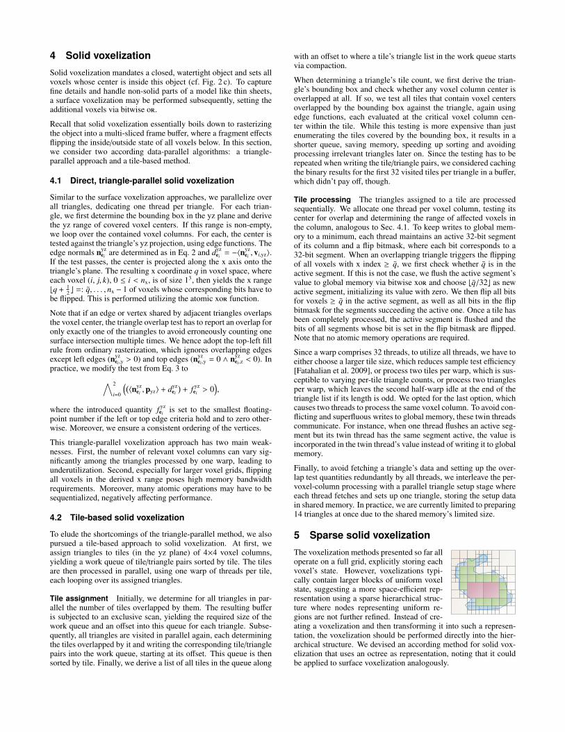
5 Sparse solid voxelization

The voxelization methods presented so far alloperate on a full grid, explicitly storing eachvoxel’s state. However, voxelizations typi-cally contain larger blocks of uniform voxelstate, suggesting a more space-efficient rep-resentation using a sparse hierarchical struc-ture where nodes representing uniform re-gions are not further refined. Instead of cre-ating a voxelization and then transforming it into such a represen-tation, the voxelization should be performed directly into the hier-archical structure. We devised an according method for solid vox-elization that uses an octree as representation, noting that it couldbe applied to surface voxelization analogously.

Because adding individual nodes on the fly during voxelization isill-suited in a massively parallel context, we create the adapted oc-tree structure up-front and subsequently populate it:

• First, all finest-level (i.e. level-0) nodes required during the vox-elization have to be determined. Since an octree node has eitherno or eight children, it sufficies to merely determine all requiredlevel-1 nodes instead (Sec. 5.1).

• Based on this node set, the whole sparse octree is then con-structed bottom-up (Sec. 5.2).

• Subsequently, the input object is voxelized into the finest-levelnodes (Sec. 5.3).

• Finally, the inside/outside parity flips are propagated hierarchi-cally to obtain a solid voxelization (Sec. 5.4).

In our implementation (cf. Fig. 6), each level-0 node stores a voxelsub-grid of size 43 for encoding and processing efficiency, thus es-sentially representing two finer levels. All nodes of one level arestored contiguously, sorted according to the Morton space-fillingcurve. Hence, a node’s eight children are contiguous in memoryand the first child has an index that is a multiple of eight. Eachnode maintains a pointer to its first child as well as pointers to itsparent and its neighbors in x direction, which help accelerating thevoxelization and propagation stages.

Morton index

Parent node

First child node

+x neighbor node

−x neighbor node

Sample index

01

2

Figure 6: Overview of the octree structure (2D analog).

5.1 Determination of active level-1 nodes

To determine the level-1 nodes overlapped by the input mesh, re-ferred to as active nodes, we could adopt a strategy similar to deriv-ing the work queue in Sec. 4.2. However, it is more space-efficientto generate a surface voxelization into a grid with level-1 resolu-tion and to extract the active voxels from it. Because all level-1nodes whose voxel region is not uniform have to be identified asactive, we perform a conservative voxelization, using the optimizedversion from Sec. 3.2 with the following modifications. First, thetriangle is shifted in +x direction by half a level-0 sub-grid (SG)voxel to account for sampling at the voxel center. Second, we en-large the triangle’s bounding box in −x direction by one SG voxeland adapt the 2D edge functions accordingly, shifting all criticalpoints that are on the voxel’s max x face in +x direction by one SGvoxel. This ensures that the final voxelization boundary consistssolely of level-0 nodes (see the node marked with ∗ in Fig. 7 for anexample).

After the level-1 voxelization is created, we derive a list of activenodes sorted in Morton order, with a node’s Morton code beingdetermined by interleaving the bits of its xyz grid position (i, j, k)(mapping it to the binary number kn−1 jn−1in−1 . . . k0 j0i0). First, welaunch one thread per 32-bit block of the voxelization. Each countsthe number of set bits and writes it to a buffer. Then a scan is runon the buffer to derive offsets into the list of active level-1 nodes(ActNodes1) as well as the list’s length. Finally, again one threadis launched per block, writing the Morton codes of the block’s setvoxels into ActNodes1, starting at its designated offset. To directlyobtain a sorted list, we use blocks of extent 4×4×2, employ theblock’s index in Morton order when accessing the buffer and thescan result, and traverse the bits within the block in Morton order.

5.2 Octree construction

Given the list ActNodes1, we then construct the sparse octree. First,the 8 length(ActNodes1) child nodes of the active level-1 nodes areallocated and initialized (Nodes0), setting the x-neighbor pointersbetween adjacent nodes with the same parent node. Subsequently,by checking the Morton codes, we determine for each active level-1node whether the next node in ActNodes1 has a different level-2parent, writing 1 if so and 0 otherwise into a buffer Flag1, which isthen subject to an exclusive scan, yielding ParentIndex1. Note thatits last entry plus one equals the number of active level-2 nodes Na

2.

We then allocate and initialize the 8Na2

level-1 nodes (Nodes1) sim-ilar to the level-0 nodes. Moreover, we establish child and parentpointers for the active level-1 nodes and their children, respectively.Here, the i-th entry in ActNodes1 corresponds to Nodes1[ j] withj = 8 ParentIndex1[i] +

(

ActNodes1[i] mod 8)

and has Nodes0[8i]as its first child.

Subsequently, a list of active level-2 nodes (ActNodes2) is derivedfrom ActNodes1 by stripping the Morton codes of the three leastsignificant bits and performing compaction, utilizing Flag1 andParentIndex1. ActNodes2 is then processed like ActNodes1 be-fore to establish the level-2 nodes. The remaining levels are treatedanalogously. In practice, we stop this process before reaching asingle root node at a level where all nodes are typically present (wechose two levels below the root node), as this later speeds up traver-sal. Consequently, all nodes at this top level n must be created, andduring initialization x-neighbor pointers are established for all ad-jacent nodes. Finally, starting at the top level, x-neighbor pointershave to be propagated from nodes in level i to their child nodes inlevel i−1, such that adjacent level-(i−1) nodes with different parentnodes are also linked.

Note that our octree construction algorithm shares several similari-ties to the approach by Zhou et al. [2010], like proceeding bottom-up in a breadth-first fashion and using Morton ordering. The maindifferences are in the stored payload, with Zhou et al. operating on agiven point cloud, as well as the adjacency information maintained,where they derive pointers to all 26 neighbors of a node.

5.3 Voxelization into octree

Once the octree is created, we voxelize the input mesh into thissparse structure, allocating one thread per triangle. As in Sec. 4,essentially a 2D rasterization in the yz plane is performed, but in-stead of flipping all relevant bits in a covered voxel column, we onlyupdate the level-0 node overlapped by the triangle and propagatethe flip to the other affected voxels in the column in a later stage.For each triangle, we first determine the bounding box and checkwhether it overlaps any SG voxel center in the yz plane. If so, wederive the yz range of level-0 voxels (tiles) containing overlappedSG voxel centers. Edge functions for overlap testing are then setup as in Sec. 4. Pursuing a two-level approach, we loop over thetiles and check for triangle overlap. If an active tile is identified, wethen loop over its 4×4 SG voxel columns, testing their centers foroverlap. In case an overlap is reported, we project the center alongthe x axis onto the triangle’s plane and derive the x index q of thefirst SG voxel that needs to be flipped. The level-0 node containingthat voxel is identified, and all voxels in the corresponding columnof its voxel sub-grid within the local x-index range (q mod 4), . . . , 3are flipped via an atomic xor operation.

To access a node, we initially perform a full descent in the octreefrom the top level. Within a tile, x-neighbor pointers are then uti-lized for fast navigation. When entering a new tile, we derive thecommon ancestor node of the previous and the desired node fromtheir Morton codes. Depending on this ancestor’s level, we eitherascent to this node and then descent or perform a full descent.

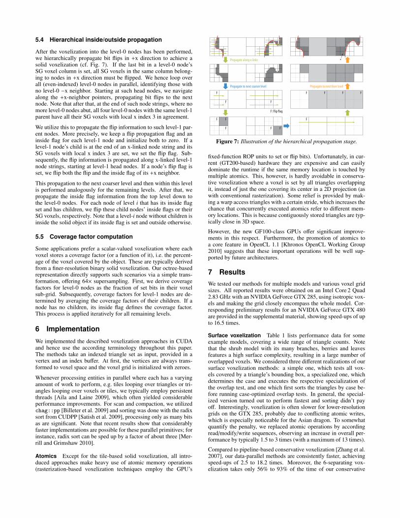
5.4 Hierarchical inside/outside propagation

After the voxelization into the level-0 nodes has been performed,we hierarchically propagate bit flips in +x direction to achieve asolid voxelization (cf. Fig. 7). If the last bit in a level-0 node’sSG voxel column is set, all SG voxels in the same column belong-ing to nodes in +x direction must be flipped. We hence loop overall (even-indexed) level-0 nodes in parallel, identifying those withno level-0 −x neighbor. Starting at such head nodes, we navigatealong the +x-neighbor pointers, propagating bit flips to the nextnode. Note that after that, at the end of such node strings, where nomore level-0 nodes abut, all four level-0 nodes with the same level-1parent have all their SG voxels with local x index 3 in agreement.

We utilize this to propagate the flip information to such level-1 par-ent nodes. More precisely, we keep a flip propagation flag and aninside flag for each level-1 node and initialize both to zero. If alevel-1 node’s child is at the end of an x-linked node string and itsSG voxels with local x index 3 are set, we set the flip flag. Sub-sequently, the flip information is propagated along x-linked level-1node strings, starting at level-1 head nodes. If a node’s flip flag isset, we flip both the flip and the inside flag of its +x neighbor.

This propagation to the next coarser level and then within this levelis performed analogously for the remaining levels. After that, wepropagate the inside flag information from the top level down tothe level-0 nodes. For each node of level i that has its inside flagset and has children, we flip these child nodes’ inside flags or theirSG voxels, respectively. Note that a level-i node without children isinside the solid object if its inside flag is set and outside otherwise.

5.5 Coverage factor computation

Some applications prefer a scalar-valued voxelization where eachvoxel stores a coverage factor (or a function of it), i.e. the percent-age of the voxel covered by the object. These are typically derivedfrom a finer-resolution binary solid voxelization. Our octree-basedrepresentation directly supports such scenarios via a simple trans-formation, offering 64× supersampling. First, we derive coveragefactors for level-0 nodes as the fraction of set bits in their voxelsub-grid. Subsequently, coverage factors for level-1 nodes are de-termined by averaging the coverage factors of their children. If anode has no children, its inside flag defines the coverage factor.This process is applied iteratively for all remaining levels.

6 Implementation

We implemented the described voxelization approaches in CUDAand hence use the according terminology throughout this paper.The methods take an indexed triangle set as input, provided in avertex and an index buffer. At first, the vertices are always trans-formed to voxel space and the voxel grid is initialized with zeroes.

Whenever processing entities in parallel where each has a varyingamount of work to perform, e.g. tiles looping over triangles or tri-angles looping over voxels or tiles, we typically employ persistentthreads [Aila and Laine 2009], which often yielded considerableperformance improvements. For scan and compaction, we utilizedchag::pp [Billeter et al. 2009] and sorting was done with the radixsort from CUDPP [Satish et al. 2009], processing only as many bitsas are significant. Note that recent results show that considerablyfaster implementations are possible for these parallel primitives; forinstance, radix sort can be sped up by a factor of about three [Mer-rill and Grimshaw 2010].

Atomics Except for the tile-based solid voxelization, all intro-duced approaches make heavy use of atomic memory operations(rasterization-based voxelization techniques employ the GPU’s

F

F

F F F

F F F F

F

F

F F

Propagate along x-links

Propagate to next coarser level Propagate to next finer level

F: Flip flag

*

Figure 7: Illustration of the hierarchical propagation stage.

fixed-function ROP units to set or flip bits). Unfortunately, in cur-rent (GT200-based) hardware they are expensive and can easilydominate the runtime if the same memory location is touched bymultiple atomics. This, however, is hardly avoidable in conserva-tive voxelization where a voxel is set by all triangles overlappingit, instead of just the one covering its center in a 2D projection (aswith conventional rasterization). Some relief is provided by mak-ing a warp access triangles with a certain stride, which increases thechance that concurrently executed atomics refer to different mem-ory locations. This is because contiguously stored triangles are typ-ically close in 3D space.

However, the new GF100-class GPUs offer significant improve-ments in this respect. Furthermore, the promotion of atomics toa core feature in OpenCL 1.1 [Khronos OpenCL Working Group2010] suggests that these important operations will be well sup-ported by future architectures.

7 Results

We tested our methods for multiple models and various voxel gridsizes. All reported results were obtained on an Intel Core 2 Quad2.83 GHz with an NVIDIA GeForce GTX 285, using isotropic vox-els and making the grid closely encompass the whole model. Cor-responding preliminary results for an NVIDIA GeForce GTX 480are provided in the supplemental material, showing speed-ups of upto 16.5 times.

Surface voxelization Table 1 lists performance data for someexample models, covering a wide range of triangle counts. Notethat the shrub model with its many branches, berries and leavesfeatures a high surface complexity, resulting in a large number ofoverlapped voxels. We considered three different realizations of oursurface voxelization methods: a simple one, which tests all vox-els covered by a triangle’s bounding box, a specialized one, whichdetermines the case and executes the respective specialization ofthe overlap test, and one which first sorts the triangles by case be-fore running case-optimized overlap tests. In general, the special-ized version turned out to perform fastest and sorting didn’t payoff. Interestingly, voxelization is often slower for lower-resolutiongrids on the GTX 285, probably due to conflicting atomic writes,which is especially noticeable for the Asian dragon. To somewhatquantify the penalty, we replaced atomic operations by accordingread/modify/write sequences, observing an increase in overall per-formance by typically 1.5 to 3 times (with a maximum of 13 times).

Compared to pipeline-based conservative voxelization [Zhang et al.2007], our data-parallel methods are consistently faster, achievingspeed-ups of 2.5 to 18.2 times. Moreover, the 6-separating vox-elization takes only 56% to 93% of the time of our conservative

Grid Pipeline-based Our conservative voxelization 6-separating voxelizationModel

size conserv. voxel. Simple Specialized Sorted #voxels 1D/2D/3D Simple Specialized Sorted #voxels

1283 10.39 1.62 1.65 2.94 54k 10%/49%/41% 1.60 1.50 2.37 33k

Stanford bunny 2563 10.24 3.99 2.51 4.19 222k 0%/20%/79% 3.38 1.98 3.16 133k

(69,666 tris) 5123 14.80 11.97 5.96 8.40 900k 0%/ 9%/91% 12.40 4.59 6.26 535k

10243 72.64 60.96 20.69 26.75 3627k 0%/ 3%/97% 58.08 17.09 18.42 2147k

1283 188.16 27.71 25.44 30.39 102k 75%/18%/ 7% 27.13 15.58 18.31 74k

Shrub 2563 236.50 22.57 17.81 23.07 426k 57%/18%/25% 21.37 10.88 13.49 274k

(751,399 tris) 5123 336.30 36.10 25.42 28.94 1705k 46%/17%/38% 34.18 15.83 16.61 1022k

10243 804.45 118.23 63.49 65.55 6776k 22%/27%/52% 110.71 40.95 35.82 3924k

1283 116.27 12.67 11.72 16.99 39k 89%/10%/ 1% 12.54 8.91 13.51 25k

Stanford dragon 2563 142.88 9.14 8.26 16.84 162k 64%/28%/ 8% 9.09 6.60 12.84 98k

(871,414 tris) 5123 194.15 10.93 10.69 20.67 660k 24%/39%/36% 10.99 8.15 15.55 387k

10243 331.81 24.17 23.00 32.18 2664k 8%/24%/68% 23.74 16.24 23.45 1539k

1283 1261.99 234.04 227.37 192.17 22k 99%/ 1%/ 0% 230.13 153.94 187.02 16k

XYZ RGB Asian dragon 2563 1496.62 111.11 106.63 134.08 91k 97%/ 3%/ 0% 108.87 76.89 113.59 61k

(7,218,906 tris) 5123 — 73.78 68.99 130.76 374k 88%/11%/ 1% 74.55 54.70 97.29 233k

10243 — 92.48 85.26 141.11 1516k 60%/32%/ 8% 95.28 66.59 105.32 897k

Table 1: Running time (in ms) for different surface voxelization methods, along with the number of resulting voxels and the encounteredpercentage of cases with a 1D, 2D and 3D bounding box. For comparison, the pipeline-based approach by Zhang et al. [2007] is included.

voxelization, mainly thanks to setting 26% to 42% fewer voxels.

Solid voxelization As the results in Table 2 show, the tile-basedmethod becomes faster than the triangle-parallel approach if thegrid size is high or the model features many triangles. In thesecases, the overhead of assigning triangles to tiles and always test-ing all voxel columns in a tile for overlap is offset by the saving inmemory bandwidth and the avoidance of atomic operations. Alsonote the effectiveness of the tile assignment stage in skipping trian-gles that don’t overlap a tile’s voxel column centers. As an extremeexample, less than 0.3% of the (typically tiny) triangles are put inthe work queue for the Asian dragon and a 1283 grid.

When compared against the fastest pipeline-based version [Eise-mann and Decoret 2008], at least one of our methods is faster inhalf of the listed cases, which is encouraging. Considering thatsolid voxelization is essentially a rasterization problem, this meanswe manage to outperform the hardware rasterizer and the blendstage for a task they were designed for. Note that as the raster-izer processes triangles sequentially, the voxelization time can bedominated by the fixed setup cost per triangle. Consequently, ourdata-parallel approaches excel for smaller grid sizes and modelswith a high triangle count.

Sparse solid voxelization Table 3 reveals that our octree-basedsolid voxelization is indeed very sparse. In particular, we are ableto represent a voxelization covering a grid of size 40963 with just216 MB (bunny model), comprising both the data and the octreestructure. This is just 2.6% of the 8 GB that would be required forrepresenting the grid explicitly. Note that our memory consumptioncan be even further decreased by storing the x-neighbor pointersseparately and getting rid of them after the voxelization process.

With respect to our full solid voxelization methods, the runningtime of the sparse approach compares favorable for the bunnymodel, performing even twice as fast for a 10242 grid. By contrast,it turns out to be more expensive for models with a higher trian-gle count, but it additionally provides an octree representation andcan support larger grid sizes. The timing break-down indicates thatthe determination of active level-1 nodes is rather costly and caneven clearly dominate the overall time (Asian dragon). Again, thismainly can be traced back to the heavy use of atomic operations.

8 Conclusion

We have presented data-parallel algorithms for both surface andsolid voxelization. Our conservative voxelization method outper-forms previous GPU-based approaches by up to one order of mag-

Grid Pipe- Tri- Tile-basedModel

size line parall. Ttotal Tpairs Tsort Ttiles #pairs #tris

1283 0.52 0.48 1.53 0.38 0.32 0.48 42k 64.2

Stanford 2563 0.58 1.48 2.02 0.39 0.44 0.80 81k 32.2

bunny 5123 1.43 9.27 4.72 0.49 0.78 2.88 145k 14.6

10243 8.75 74.86 18.24 0.76 1.39 14.08 301k 7.6

1283 2.69 1.45 2.51 1.09 0.32 0.47 40k 81.8

Stanford 2563 2.73 2.03 4.72 1.21 0.64 1.11 156k 84.7

dragon 5123 3.16 7.57 7.19 1.41 1.96 2.91 476k 67.3

10243 13.56 51.95 16.41 1.79 3.54 8.76 944k 34.0

1283 18.30 8.84 7.70 5.06 0.19 0.44 21k 81.5

Asian 2563 18.35 8.82 8.73 5.48 0.44 0.75 84k 89.1

dragon 5123 18.52 13.77 12.63 6.66 1.47 2.18 342k 96.3

10243 20.46 50.94 24.26 7.66 4.91 7.92 1366k 99.6

Table 2: Running time (in ms) for different solid voxelization meth-ods. The break-down for the tile-based approach considers deter-mining the work queue (Tpairs), sorting it (Tsort), and processing thetiles (Ttiles). Moreover, the number of tile/triangle pairs in the queueand the average triangle list length per active tile are provided.

nitude, making it accessible to real-time applications. It employsa new triangle/box overlap test that should also be useful in otherdomains. Moreover, our algorithm easily can be adapted to a dif-ferent overlap criterion, as we have shown by introducing a fast6-separating surface voxelization method.

Two strategies for solid voxelization have been demonstrated. Theirunderlying approaches offer data-parallel alternatives to the hard-ware rasterizer and compare favorable in many cases. In particular,our tile-based method provides an efficient solution for rasterizationtasks where larger amounts of data may be updated per fragment(e.g. color and depth, which cannot be done with a single atomicoperation).

Finally, an octree-based sparse voxelization approach has been in-troduced that offers a compact hierarchical representation and al-lows voxelizations of resolutions not possible before on GPUs. Itbasically constitutes an alternative, domain-adapted, custom ren-dering pipeline that surpasses previous limitations, enabling the di-rect rendering into a sparse spatial data structure. An interestingavenue for future work is applying this strategy to other tasks wherethe standard rasterization pipeline proves too restrictive.

Acknowledgements

The (original) bunny and dragon models are courtesy of the Stan-ford 3D scanning repository; the shrub model is from the Xfrogpublic plants library.

Model Stanford bunny Stanford dragon XYZ RGB Asian dragon

Binary grid size 5123 10243 20483 40963 5123 10243 20483 40963 5123 10243 20483 40963

Scalar-valued grid size 1283 2563 5123 10243 1283 2563 5123 10243 1283 2563 5123 10243

Total 4.87 9.15 25.17 93.27 14.50 23.59 37.71 100.32 47.71 102.96 143.90 178.40

Determine active level-1 nodes 1.49 1.92 3.60 12.74 8.07 10.63 9.02 17.79 27.07 80.91 101.09 77.79

Construct octree 1.01 1.74 3.99 12.36 0.97 1.52 3.37 9.43 0.90 1.35 2.37 6.04

Voxelize into octree 1.47 3.43 10.65 42.61 4.45 9.59 20.57 55.36 17.35 17.96 35.81 82.55

Propagate inside/outside 0.44 1.36 5.12 19.71 0.32 0.92 3.28 13.16 0.23 0.56 1.98 7.54

Compute coverage factor 0.12 0.37 1.37 5.36 0.10 0.28 1.02 3.98 0.07 0.18 0.60 2.29

Stored level-0 nodes 5.30% 2.71% 1.37% 0.69% 3.82% 2.00% 1.01% 0.51% 2.02% 1.10% 0.57% 0.29%

Octree size 3.2 MB 13.2 MB 53.7 MB 216 MB 2.3 MB 9.7 MB 39.6 MB 159 MB 1.2 MB 5.3 MB 22.3 MB 90.8 MB

Table 3: Running time (in ms) for our sparse solid voxelization method, including a break-down. The percentage of explicitly stored level-0nodes provides a measure of sparseness. The given octree size accounts for both the structure and the data.

References

Abrash, M. 2009. Rasterization on Larrabee. Dr. Dobb’s.http://www.drdobbs.com/high-performance-computing/217200602.

Aila, T., and Laine, S. 2009. Understanding the efficiency of raytraversal on GPUs. In Proceedings of High Performance Graph-ics 2009, 145–149.

Akenine-Moller, T., and Aila, T. 2005. Conservative and tiled ras-terization using a modified triangle set-up. Journal of GraphicsTools 10, 3, 1–8.

Akenine-Moller, T. 2001. Fast 3D triangle-box overlap testing.Journal of Graphics Tools 6, 1, 29–33.

Billeter, M., Olsson, O., andAssarsson, U. 2009. Efficient streamcompaction on wide SIMD many-core architectures. In Proceed-ings of High Performance Graphics 2009, 159–166.

Cohen-Or, D., and Kaufman, A. 1995. Fundamentals of surfacevoxelization. Graphical Models and Image Processing 57, 6,453–461.

Dong, Z., Chen, W., Bao, H., Zhang, H., and Peng, Q. 2004. Real-time voxelization for complex models. In Proceedings of PacificGraphics 2004, 43–50.

Eisemann, E., and Decoret, X. 2006. Fast scene voxelization andapplications. In Proceedings of ACM SIGGRAPH Symposium onInteractive 3D Graphics and Games 2006, 71–78.

Eisemann, E., and Decoret, X. 2008. Single-pass GPU solid vox-elization for real-time applications. In Proceedings of GraphicsInterface 2008, 73–80.

Eisenacher, C., and Loop, C. 2010. Data-parallel micropolygonrasterization. In Eurographics 2010 Short Papers, 53–56.

Fang, S., and Chen, H. 2000. Hardware accelerated voxelization.Computers & Graphics 24, 3, 433–442.

Fatahalian, K., Luong, E., Boulos, S., Akeley, K., Mark, W. R.,and Hanrahan, P. 2009. Data-parallel rasterization of microp-olygons with defocus and motion blur. In Proceedings of HighPerformance Graphics 2009, 59–68.

Haines, E. A., andWallace, J. R. 1991. Shaft culling for efficientray-cast radiosity. In Proceedings of Eurographics Workshop onRendering 1991, 122–138.

Hasselgren, J., Akenine-Moller, T., and Ohlsson, L. 2005. Con-servative rasterization. In GPU Gems 2, M. Pharr, Ed. AddisonWesley Professional, ch. 42, 677–690.

Huang, J., Yagel, R., Filippov, V., and Kurzion, Y. 1998. An accu-rate method for voxelizing polygon meshes. In Proceedings ofIEEE Symposium on Volume Visualization 1998, 119–126.

Ivson, P., Duarte, L., and Celes, W. 2009. GPU-accelerated uni-form grid construction for ray tracing dynamic scenes. Tech.Rep. 14/09, Pontifıcia Universidade Catolica do Rio de Janeiro.

Kalojanov, J., and Slusallek, P. 2009. A parallel algorithm for con-struction of uniform grids. In Proceedings of High PerformanceGraphics 2009, 23–28.

Khronos OpenCL Working Group. 2010. The OpenCL Specifica-tion. Version: 1.1.

Lauterbach, C., Garland, M., Sengupta, S., Luebke, D., andManocha, D. 2009. Fast BVH construction on GPUs. Com-puter Graphics Forum 28, 2, 375–384.

Li, W., Fan, Z., Wei, X., and Kaufman, A. 2005. Flow simula-tion with complex boundaries. In GPU Gems 2, M. Pharr, Ed.Addison Wesley Professional, ch. 47, 747–764.

Liu, F., Huang, M.-C., Liu, X.-H., andWu, E.-H. 2010. FreePipe: aprogrammable parallel rendering architecture for efficient multi-fragment effects. In Proceedings of ACM SIGGRAPH Sympo-sium on Interactive 3D Graphics and Games 2010, 75–82.

Merrill, D., and Grimshaw, A. 2010. Revisiting sorting forGPGPU stream architectures. Tech. Rep. CS2010-03, Depart-ment of Computer Science, University of Virginia.

Nichols, G., Penmatsa, R., and Wyman, C. 2010. Interactive,multiresolution image-space rendering for dynamic area light-ing. Computer Graphics Forum 29, 4, 1279–1288.

Pineda, J. 1988. A parallel algorithm for polygon rasterization.Computer Graphics (Proceedings of SIGGRAPH 88) 22, 4, 17–20.

Reinbothe, C. K., Boubekeur, T., and Alexa, M. 2009. Hybridambient occlusion. In Eurographics 2009 Annex (Areas Papers),51–57.

Satish, N., Harris, M., and Garland, M. 2009. Designing ef-ficient sorting algorithms for manycore GPUs. In Proceedingsof IEEE International Parallel & Distributed Processing Sympo-sium 2009, 1–10.

Seiler, L., Carmean, D., Sprangle, E., Forsyth, T., Abrash, M.,Dubey, P., Junkins, S., Lake, A., Sugerman, J., Cavin, R., Es-pasa, R., Grochowski, E., Juan, T., and Hanrahan, P. 2008.Larrabee: A many-core x86 architecture for visual computing.ACM Transactions on Graphics 27, 3, 18:1–18:15.

Sun, X., Zhou, K., Stollnitz, E., Shi, J., andGuo, B. 2008. Interac-tive relighting of dynamic refractive objects. ACM Transactionson Graphics 27, 3, 35:1–35:9.

Zhang, L., Chen, W., Ebert, D. S., and Peng, Q. 2007. Conservativevoxelization. The Visual Computer 23, 9–11, 783–792.

Zhou, K., Hou, Q., Wang, R., and Guo, B. 2008. Real-time KD-tree construction on graphics hardware. ACM Transactions onGraphics 27, 5, 126:1–126:9.

Zhou, K., Gong, M., Huang, X., and Guo, B. 2010. Data-paralleloctrees for surface reconstruction. IEEE Transactions on Visual-ization and Computer Graphics. To appear.