
Fast Neighborhood Search for the Nesting Problem1 · 2011-10-17 · Fast Neighborhood Search for...
109
Fast Neighborhood Search for the Nesting Problem 1 Benny Kjær Nielsen and Allan Odgaard {benny, duff}@diku.dk February 14, 2003 1 Technical Report no. 03/02, DIKU, University of Copenhagen, DK-2100 Copenhagen Ø, Denmark.
Transcript of Fast Neighborhood Search for the Nesting Problem1 · 2011-10-17 · Fast Neighborhood Search for...

Fast Neighborhood Search for the Nesting Problem1
Benny Kjær Nielsen and Allan Odgaard
{benny, duff}@diku.dk
February 14, 2003
1Technical Report no. 03/02, DIKU, University of Copenhagen, DK-2100 Copenhagen Ø, Denmark.


Contents
1 Introduction 5
2 The Nesting Problem 72.1 Problem definitions . . . . . . . . . . . . . . . . . . . . . . . . . . . . . . . . . . 7
2.2 Geometric aspects . . . . . . . . . . . . . . . . . . . . . . . . . . . . . . . . . . 102.3 Existing solution methods . . . . . . . . . . . . . . . . . . . . . . . . . . . . . . 13
2.4 Legal placement methods . . . . . . . . . . . . . . . . . . . . . . . . . . . . . . 152.5 Relaxed placement methods . . . . . . . . . . . . . . . . . . . . . . . . . . . . . 172.6 Commercial solvers . . . . . . . . . . . . . . . . . . . . . . . . . . . . . . . . . . 18
2.7 3D nesting . . . . . . . . . . . . . . . . . . . . . . . . . . . . . . . . . . . . . . . 19
3 Solution Methods 23
3.1 Local search . . . . . . . . . . . . . . . . . . . . . . . . . . . . . . . . . . . . . . 243.2 Guided Local Search . . . . . . . . . . . . . . . . . . . . . . . . . . . . . . . . . 263.3 Initial solution . . . . . . . . . . . . . . . . . . . . . . . . . . . . . . . . . . . . 28
3.4 Packing strategies . . . . . . . . . . . . . . . . . . . . . . . . . . . . . . . . . . 28
4 Fast Neighborhood Search 31
4.1 Background . . . . . . . . . . . . . . . . . . . . . . . . . . . . . . . . . . . . . . 314.2 A special formula for intersection area . . . . . . . . . . . . . . . . . . . . . . . 32
4.2.1 Vector fields . . . . . . . . . . . . . . . . . . . . . . . . . . . . . . . . . . 32
4.2.2 Segment and vector field regions . . . . . . . . . . . . . . . . . . . . . . 334.2.3 Signed boundaries and shapes . . . . . . . . . . . . . . . . . . . . . . . . 354.2.4 The Intersection Theorem . . . . . . . . . . . . . . . . . . . . . . . . . . 37
4.2.5 A simple example . . . . . . . . . . . . . . . . . . . . . . . . . . . . . . 404.3 Transformation algorithms . . . . . . . . . . . . . . . . . . . . . . . . . . . . . . 42
4.4 Translation of polygons . . . . . . . . . . . . . . . . . . . . . . . . . . . . . . . 464.5 Rotation of polygons . . . . . . . . . . . . . . . . . . . . . . . . . . . . . . . . . 48
5 Miscellaneous Constraints 535.1 Overview . . . . . . . . . . . . . . . . . . . . . . . . . . . . . . . . . . . . . . . 535.2 Quality areas . . . . . . . . . . . . . . . . . . . . . . . . . . . . . . . . . . . . . 56
5.3 Margins between polygons . . . . . . . . . . . . . . . . . . . . . . . . . . . . . . 575.3.1 A straightforward solution . . . . . . . . . . . . . . . . . . . . . . . . . . 575.3.2 Rounding the corners . . . . . . . . . . . . . . . . . . . . . . . . . . . . 59
5.3.3 Self intersections . . . . . . . . . . . . . . . . . . . . . . . . . . . . . . . 595.4 Minimizing cutting path length . . . . . . . . . . . . . . . . . . . . . . . . . . . 61
3

6 3D Nesting 636.1 A generalization . . . . . . . . . . . . . . . . . . . . . . . . . . . . . . . . . . . 636.2 The straightforward approach . . . . . . . . . . . . . . . . . . . . . . . . . . . . 636.3 Reducing the number of breakpoints . . . . . . . . . . . . . . . . . . . . . . . . 67
7 Implementation Issues 737.1 General information . . . . . . . . . . . . . . . . . . . . . . . . . . . . . . . . . 737.2 Input description . . . . . . . . . . . . . . . . . . . . . . . . . . . . . . . . . . . 737.3 Slab counting . . . . . . . . . . . . . . . . . . . . . . . . . . . . . . . . . . . . . 737.4 Incorporating penalties in translation . . . . . . . . . . . . . . . . . . . . . . . . 777.5 Handling non-rectangular material . . . . . . . . . . . . . . . . . . . . . . . . . 787.6 Approximating stencils . . . . . . . . . . . . . . . . . . . . . . . . . . . . . . . . 807.7 Center of a polygon . . . . . . . . . . . . . . . . . . . . . . . . . . . . . . . . . 82
8 Computational Experiments 858.1 2D experiments . . . . . . . . . . . . . . . . . . . . . . . . . . . . . . . . . . . . 85
8.1.1 Strategy . . . . . . . . . . . . . . . . . . . . . . . . . . . . . . . . . . . . 858.1.2 Data instances . . . . . . . . . . . . . . . . . . . . . . . . . . . . . . . . 858.1.3 Lambda . . . . . . . . . . . . . . . . . . . . . . . . . . . . . . . . . . . . 878.1.4 Approximations . . . . . . . . . . . . . . . . . . . . . . . . . . . . . . . . 878.1.5 Strip length strategy . . . . . . . . . . . . . . . . . . . . . . . . . . . . . 888.1.6 Quality requirements . . . . . . . . . . . . . . . . . . . . . . . . . . . . . 928.1.7 Comparisons with published results . . . . . . . . . . . . . . . . . . . . 928.1.8 Comparisons with a commercial solver . . . . . . . . . . . . . . . . . . . 94
8.2 3D experiments . . . . . . . . . . . . . . . . . . . . . . . . . . . . . . . . . . . . 958.2.1 Data instances . . . . . . . . . . . . . . . . . . . . . . . . . . . . . . . . 958.2.2 Statistics . . . . . . . . . . . . . . . . . . . . . . . . . . . . . . . . . . . 958.2.3 Benchmarks . . . . . . . . . . . . . . . . . . . . . . . . . . . . . . . . . . 98
9 Conclusions 101
A Placements 107
4

Chapter 1
Introduction
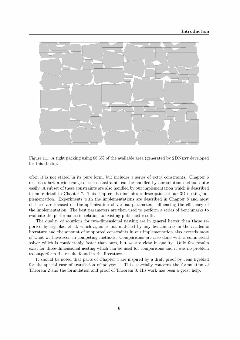
The main subject of this thesis is the so-called nesting problem, which (in short) is the problemof packing arbitrary two-dimensional shapes within the boundaries of some container. Theobjective can vary e.g. minimizing the size of a rectangular container or maximizing the numberof shapes in the container, but the core problem is to pack the shapes tightly without anyoverlap. An example of a tight packing is shown in Figure 1.1.
A substantial amount of literature has been written about this problem, where most of it hasbeen written within the past decade. A survey of the existing literature is given in Chapter 2along a detailed description of different problem types and various geometric approaches tothese problems. At the end of the chapter a three-dimensional variant of the problem isdescribed and the more limited amount of literature in this area is also discussed.
The rest of the thesis is focused on solving the nesting problem with a meta heuristicmethod called Guided Local Search (GLS). It is a continuation of the work presented in awritten report (in Danish) by Jens Egeblad and ourselves [28], which again is a continuationof the work presented in an article by Færø et al. [32]. Throughout this thesis we will oftenrefer to the work done by Jens Egeblad and ourselves (Egeblad et al. [28]).
Chapter 3 presents GLS and some other issues regarding the basics of our solution method.Most importantly the neighborhood for the local search is presented — it is a fast search ofthis neighborhood which is the major strength of our approach to the nesting problem.
Færø et al. successfully applied the GLS meta heuristic to the rectangular bin packingproblem in both two and three dimensions. The speed of their approach was especially due toa simple and very fast translation algorithm which could find the optimal (minimum overlap)axis-aligned placement of a given box. Egeblad et al. [28] realized that a similar algorithm waspossible for translating arbitrary polygons. However, they did not prove the correctness of thealgorithm.
A major part of this thesis (Chapter 4) is dedicated to such a proof. The proof is statedin general terms and translation and polygons are introduced at a very late stage. By doingthis it is simultaneously shown that the algorithm could be useful for other transformationsor other shapes. At the end of the chapter some additional work is done to adapt the generalscheme to an algorithm for rotation of polygons.
Although not explicitly proven it is easy to see that the fast translation and rotationalgorithms are also possible for three dimensions. A description of how to do this in practicefor translation is given separately in Chapter 6.
The two-dimensional nesting problem appears in a range of different industries and quite
5
Introduction
Figure 1.1: A tight packing using 86.5% of the available area (generated by 2DNest developedfor this thesis).
often it is not stated in its pure form, but includes a series of extra constraints. Chapter 5discusses how a wide range of such constraints can be handled by our solution method quiteeasily. A subset of these constraints are also handled by our implementation which is describedin more detail in Chapter 7. This chapter also includes a description of our 3D nesting im-plementation. Experiments with the implementations are described in Chapter 8 and mostof these are focused on the optimization of various parameters influencing the efficiency ofthe implementation. The best parameters are then used to perform a series of benchmarks toevaluate the performance in relation to existing published results.
The quality of solutions for two-dimensional nesting are in general better than those re-ported by Egeblad et al. which again is not matched by any benchmarks in the academicliterature and the amount of supported constraints in our implementation also exceeds mostof what we have seen in competing methods. Comparisons are also done with a commercialsolver which is considerably faster than ours, but we are close in quality. Only few resultsexist for three-dimensional nesting which can be used for comparisons and it was no problemto outperform the results found in the literature.
It should be noted that parts of Chapter 4 are inspired by a draft proof by Jens Egebladfor the special case of translation of polygons. This especially concerns the formulation ofTheorem 2 and the formulation and proof of Theorem 3. His work has been a great help.
6

Chapter 2
The Nesting Problem
2.1 Problem definitions
The term nesting has been used to describe a wide variety of two-dimensional cutting andpacking problems. They all involve a non-overlapping placement of a set of irregular two-dimensional shapes within some region of two-dimensional space, but the objective can vary.Most problems can be categorized as follows (also see the illustration in Figure 2.1):
• Decision problem. Decide whether a set of shapes fit within a given region.
• Knapsack problem. Given a set of shapes and a region, find a placement of a subset ofshapes that maximizes the utilization (area covered) of the region.
• Bin packing problem. Given a set of shapes and a set of regions, minimize the numberof regions needed to place all shapes.
• Strip packing problem. Given a set of shapes and a width W , minimize the length of arectangular region with width W such that all shapes are contained in the region.
An interesting problem type, which is not included in the above list, is a variant of the strippacking problem that deals with repeated patterns i.e. the packing layout is going to be reusedon some material repeatedly in 1 or 2 directions. With one direction of repetition this problemcan be interpreted as a nesting problem on the outside of a cylinder, where the objective isto minimize the radius. We will get back to this variation in Chapter 5. We will denote thisproblem the repeated pattern problem.
As noted the region used for strip packing is rectangular and a typical example would bea cloth-strip in the textile industry. All other regions can have any shape. It could be animalhides in the leather industry, rectangular plates in the metal industry or tree boards in thefurniture industry.
Note that all of the problems have one-dimensional counterparts, but the one-dimensionaldecision and strip packing problems are trivial to solve.
In this thesis the focus is on the decision problem, but this is not a major limitation.Heuristic solution methods for bin/knapsack/strip packing can easily be devised when givena (heuristic) solution method for the decision problem, e.g. by fixing the strip length or thenumber of bins and then solve the decision problem and if it is a success then the strip can beshortened or the number of bins decreased and vice versa if it fails. When to do what is not
7

2.1. Problem definitions The Nesting Problem
a b
Figure 2.1: a) Most variants of the nesting problem is the problem of packing shapes withinsome region(s) without overlap (decision, knapsack and bin packing). b) The strip packingvariant asks for a minimization of the length of a rectangular region.
a trivial problem and we will briefly get back to this in Section 3.4. It is important to notethat the various packing problems can also be solved in more direct ways, which could be moreefficient. Nevertheless, our focus is mainly on the decision problem.
In industrial settings a multitude of additional constraints are very often necessary, e.g. theshapes or regions can have different quality zones or even holes (animal hides). Historically,the clothing industry has had special attention. But even though this industry introduces amultitude of possible extra constraints to the problem, these constraints are often not includedin the published solution methods. An exception is Lengauer et al. [35, 37] who describe andhandle a long range of the possible additional constraints posed in the leather and the textileindustry. But most of the existing literature does not handle any additional constraints. Wewill not consider them any further in this chapter and instead a more detailed discussion ofvarious constraints (in relation to our solution method) is postponed to Chapter 5.
As indicated above the nesting problem occurs in a number of industries and it seems tohave gotten just as many names. In the clothing industry it is usually called marker making,while the metal industry prefers to call it blank nesting or simply nesting. There is no consensusin the existing literature either. Some call the shapes irregular, others call them non-convex.In a theoretical context the problem is most often called the two-dimensional irregular cuttingstock problem. This is quite verbose and therefore it is quite natural that shorter variants havebeen preferred such as polygon placement, polygon containment and (irregular) nesting. Thesenames also indicate that the irregular shapes are almost always restricted to being polygons.A quick look at the reference list in this thesis emphasizes the diversity in the naming of thisproblem.
8

The Nesting Problem 2.1. Problem definitions
In relation to Dyckhoff’s [25] typology we are dealing with problems of types 2/V/OID/M— many small differently shaped figures packed in one or several identical/different largeshape(s) in 2 dimensions.
Our general choice of wording follows below. None of the words imply any restrictions onthe shapes involved.
• Nesting. A short name for the problem, which is often used in the existing literature.
• Stencil1. A domain specific name for the pieces/shapes/polygons to be packed.
• Material. A general word for the packing region which can be used to describe garments,metal plates, wood, glass and more.
• Placement. The positioning of a set of stencils on the material. A legal placement is aplacement without any overlapping stencils and all stencils placed within the limits ofthe material.
Not surprisingly, the nesting problem is NP-hard. Most existing articles state this fact,but only few have a reference. Some refer to Fowler et al. [31] who specify a very constrainedvariant, BOX-PACK, as the following problem: Determine whether a given set of identicalboxes (integer squares) can be placed (without rotation) at integer coordinates inside a regionin the plane (not necessarily connected) without overlapping. They prove that BOX-PACKis NP-complete by making a polynomial-time reduction of 3-SAT which is the problem ofdetermining whether a Boolean formula in conjunctive normal form with 3 literals per clauseis satisfiable.
Note that the region defined in the BOX-PACK problem is not required to be connected.This means that the region could be a set of regions thus the problem also covers the binpacking problem. Also note that the 1-dimensional variant of BOX-PACK is a trivial problemto solve. This is not true for less constrained variants of the nesting problem.
The majority of articles related to nesting only handle rectangular materials and this isa constraint which is not included in the BOX-PACK problem. If it was then the problem(packing identical squares in a rectangle) would no longer be NP-hard. It would have a trivialsolution. Some authors seem to have missed this point (e.g. [35, 36]).
To remedy this situation we define a new problem, BOX-PACK-2: Determine whethera given set of integer rectangles (not necessarily identical) can be placed (without rotation)inside a rectangular region without overlapping. Inspired by the proof in [49]:
Theorem 1. BOX-PACK-2 is NP-complete.
Proof. We are going to make a polynomial-time reduction of 1-dimensional bin packing [33].The bin packing problem can be stated as follows: Given a finite set of integers X, a
bin capacity B and an integer K, determine whether we can partition X into disjoint setsX1, ..., XK such that the sum of integers in each Xi is less than or equal to B.
Now replace each integer x ∈ X with a rectangle of height 1 and width x and use a givenalgorithm to solve BOX-PACK-2 to place these rectangles in a rectangle of width B and height
1Stencil, n. [Probably from OF. estincelle spangle, spark, F. [’e]tincelle spark, L. scintilla. See Scintillate,and cf. Tinsel.] A thin plate of metal, leather, or other material, used in painting, marking, etc. The pattern iscut out of the plate, which is then laid flat on the surface to be marked, and the color brushed over it. Calledalso stencil plate. Source: Webster’s Revised Unabridged Dictionary, 1996, 1998 MICRA, Inc.
9

2.2. Geometric aspects The Nesting Problem
a b
Figure 2.2: The degree of overlap can be measured in various ways. Here are two examples:a) The precise area of the overlap. b) The horizontal intersection depth.
K. By post processing this solution (e.g. sliding the rectangles down and to the left) we willget a solution to the bin packing problem by using the width of the rectangles in each row asthe integers in each bin.
Clearly, BOX-PACK-2 is also in NP and thereby NP-complete.
2.2 Geometric aspects
Before we proceed with a description and discussion of some of the existing solution methods,we will describe some of the different approaches to the geometric aspects of the nestingproblem. In this section only polygons are considered since most solution methods can onlyhandle these.
The basic requirement is to produce solutions with no overlap between polygons. Thismeans that either the polygons must be placed without creating overlap or it should be possibleto detect and eventually remove any overlap occurring in the solution process.
If overlap is allowed as part of the solution process then there is a lot of diversity in thegeometric approaches to the problem. Given two polygons P and Q, one or more of thefollowing problems need to be handled.
• Do P and Q intersect?
• If P and Q intersect, how much do they intersect?
• If P and Q do not intersect, how far are they apart?
The question of the size of an overlap is handled in very different ways. The most naturalway is to measure the exact area of the overlap (see Figure 2.2a). This can be an expensivecalculation and thus quite a few alternatives have been tried. Oliveira and Ferreira [50] usedthe area of the smallest rectangle containing the intersection, but this has probably not savedmuch time since the hard part is to find the intersection points and not to do the calculationof the area. It has also been suggested to use the intersection depth (see Figure 2.2b), whichmakes sense since the depth of the intersection also expresses how much one of the polygonsmust be moved to avoid the overlap. Dobkin et al. [21] describe an algorithm to get theminimum intersection depth i.e. they also find the direction that results in the smallest possibleintersection depth. Unfortunately they require one of the polygons to be convex.
The distance between two polygons, which are not intersecting, can be useful if they areto be moved closer together. But most algorithms are more focused on the relations betweenpolygons and empty areas. Dickinson and Knopf [19] introduce a moment based metric forboth 2D and 3D. This metric is based on evaluating the compactness of the remaining free
10

The Nesting Problem 2.2. Geometric aspects
Reference point
Q
P
Figure 2.3: Example of the No-Fit-Polygon (thick border) of stencil P in relation to stencil Q.The reference point of P is not allowed inside the NFP if overlap is to be avoided.
space in an unfinished placement. They use this to implement a sequential packing algorithmin 3D [18].
Some theoretical work has also been done by Stoyan et al. [54] on defining a so-calledΦ-function. Such a function can differentiate between three states of polygon interference;intersection, disjunction and touching. But again, they only handle convex polygons.
Solution methods which do not involve any overlapping polygons at any time in the solutionprocess almost always use the concept of the No-Fit-Polygon (NFP). It is often claimed to havebeen introduced by Art [4], which is not entirely correct. The NFP is a polygon which describesthe legal/illegal placements of one polygon in relation to another polygon. Art introduced andused the envelope, which is a polygon that describes the legal/illegal placements of a polygonin relation to the packing done so far. The calculations are basically the same and they arestrongly connected with the so-called Minkowski sum.
Given two polygons P and Q the construction of the NFP of P in relation to Q can befound in the following way: Choose a reference point for P . Slide P around Q as close aspossible without intersecting. The trace of the reference point is the contour of the NFP.An example can be seen in Figure 2.3. To determine whether P and Q intersect it is onlynecessary to determine whether the reference point of P is inside or outside their NFP. Butthe real benefit of the NFP is when the polygons are to be placed closely together. This can bedone by placing the reference point of P at one of the edges of the NFP. If P and Q have s andt edges, respectively, then the number of edges in their NFP will be in the order of O(s2t2) [5].
The NFP has one major weakness. It has to be calculated for all pairs of polygons. Ifthe polygons are not allowed to be rotated this is not a big problem since it can be done in apreprocessing step in a reasonable time given that the number n of differently shaped polygonsis not too large (requiring n2 NFPs). But if a set of rotation angles and/or flipping are allowedthen even more NFPs have to be calculated e.g. 4 rotation angles and flipping would requirethe calculation of (4 · 2 · n)2 NFPs. It is still a quadratic expression, but even a small numberof polygons would require a large number of NFPs e.g. 4 polygons would require 1024 NFPs.If free rotation was needed then an approximate solution method using a large number ofrotation angles would not be a viable approach. Nevertheless NFPs are still a powerful toolfor restricted problems.
11

2.2. Geometric aspects The Nesting Problem
Figure 2.4: The raster model requires all stencils to be defined by a set of grid squares. Thedrawing above is an example of a polygon and its equivalent in a raster model.
A fundamentally different solution to the geometric problems is what some authors call theraster model [45, 50, 35]. This is a discrete model of the polygons (which then do not haveto be polygons), created by introducing a grid of some size to represent the material i.e. eachpolygon covers some set of raster squares. The polygons can then be represented by matrices.An example of a polygon and its raster model equivalent is given in Figure 2.4.
Translations in the raster model are very simple while rotations are quite difficult. Anoverlap calculation takes at least linear time in the number of raster lines involved and thisalso clearly shows the weakness of this approach. A low granularity of the raster model providesfast calculations at the expense of little precision. A high granularity will result in very slowcalculations. Comparisons with the polygonal model was done by Heckmann and Lengauer [35]and they concluded that the polygonal model was the better choice for their purposes.
With the exception of the calculation of the intersection area of overlapping polygons,none of the methods described above handle rotation efficiently. This is also reflected in thepublished articles which rarely handle more than steps of 180◦ or 90◦ rotation. Free rotationis usually handled in a brute-force discrete manner i.e. by calculating overlap for a large set ofrotation angles and then select a minimum.
A more sophisticated approach for rotation has been published by Milenkovic [47]. Heuses mathematical programming in a branch-and-bound context to solve very small rotationalcontainment problems to near-optimality2. Very small is in the order of 2-3 polygons. Li andMilenkovic [43] have used mathematical programming to make precise local adjustments of asolution, so-called compaction and separation. This could be useful in combination with othernesting techniques.
2Given a set of polygons and a container, find rotations and translations that place the polygons in thecontainer without any overlaps.
12

The Nesting Problem 2.3. Existing solution methods
2.3 Existing solution methods
There exists a substantial amount of literature about two-dimensional cutting and packingproblems, but most of it is focused on the rectangular variant. A recent survey has beenwritten by Lodi et al. [44] about these restricted problems and this includes references to othersurveys. In the following we are going to focus on articles about irregular nesting problems.
Most articles about the nesting problem has been written within the past decade. Thereason for this is unlikely to be a lack of interest since the industrial uses are numerous asindicated in the section above. It is more likely that the necessary computing power for theneeded amount of geometric computations simply was not available until the beginning ofthe 90’s. Far more work has been done on the geometrically much easier problem of packingrectangles (or 3D boxes).
The strip packing problem is the problem most often handled. In the following it is implic-itly assumed that the articles handle this problem, but most of the methods described couldeasily be adapted to some of the other problem types. When other problems than strip packingare handled it will be explicitly noted.
Lower bounds have not received much attention either3 — with the exception of recentwork by Heckmann and Lengauer [36]. Unfortunately their method is not applicable for morethan about 12 stencils. By selecting a subset of stencils it can also produce lower bounds forlarger sets of stencils, but the quality of the bound will not be good unless there is only a smallnumber of large stencils in the original set.
Milenkovic [48] describes an algorithm which can solve the densest translation lattice pack-ing for a very small number of stencils — not more than 4. This is the problem which we havedenoted the repeated pattern problem (in two dimensions).
Most articles are focused on heuristic methods. Basically, they can be divided into twogroups. Those only considering legal placements in the solution process and those allowingoverlap to occur during the solution process.
Several surveys have been written. Dowsland and Dowsland [22] focus explicitly on irregularnesting problems, while other surveys [26, 38] focus on a wider range of cutting and packingproblems. The latter of these is strictly focused on the use of meta-heuristic methods. Adetailed discussion of meta-heuristic algorithms applied to irregular nesting problems can befound in the introductory sections of Bennell and Dowsland [6]. Finally, a very extensive list ofreferences can be found in Heistermann and Lengauer [37], although most of them are aboutvery restricted problems — e.g. rectangular shapes.
In the following paragraphs, we will discuss some of the heuristic methods described in theexisting literature. This is far from a complete survey of applied methods, but it does includemost of the interesting (published) methods.
The methods can be divided into two basically different groups.
• Legal placement methods
These methods never violate the overlap constraint. An immediate consequence is thatplacement of a stencil must always be done in an empty part of the material.
Some of the earliest algorithms doing this only place each stencil once. According to somemeasures describing the stencils and the placement done so far, the next best stencil is
3A very simple lower bound can be based on the total area of all stencils, but it will usually be far from theoptimal solution.
13

2.3. Existing solution methods The Nesting Problem
chosen and placed. This is a fast method, but the quality of the solution is limited sinceno backtracking is done.
Most methods for strip packing follow the basic steps below:
1. Determine a sequence of stencils. This can be done randomly or by sorting thestencils according to some measure e.g. the area or the degree of convexity.
2. Place the stencils with some first/best fit algorithm. Typically a stencil is placedat the contour of the stencils already placed (using an NFP). Some algorithms alsoallow hole-filling i.e. placing a stencil in an empty area between already placedstencils.
3. Evaluate the length of the solution. Exit with this solution or change the sequenceof stencils e.g. randomly or by using some meta-heuristic method and repeat step 2.
Unfortunately the second step is very expensive and these algorithms can easily end upspending time on making almost identical placements.
Legal placement methods not doing a sequential placement do exist. These methodstypically construct a legal initial solution and then introduce some set of moves (e.g.swapping two stencils) that can be controlled by a meta heuristic method to e.g. minimizethe length of a strip. Examples are Burke and Kendall [12, 10, 11] (simulated annealing,ant algorithms and evolutionary algorithms) and Blazewicz et al. [8] (Tabu Search). Thelatter is also interesting because it allows a set of rotation angles.
• Relaxed placement methods
The obvious alternative is to allow overlaps to occur as part of the solution process. Theobjective is then to minimize the amount of overlap. A legal placement has been foundwhen the overlap reaches 0.
In this context it is very easy to construct an initial placement. It can simply be arandom placement of all of the stencils, although it might be better to start with abetter placement than that.
Searching for a minimum overlap can be done by iteratively improving the placementi.e. decrease the total overlap. This is typically done by moving/rotating stencils. Theneighborhood of solutions can be defined in various ways, but all existing solution meth-ods have restricted the translational moves to some set of horizontal and vertical trans-lations.
Clearly the relaxed placement methods has to handle a larger search space than the legalplacement methods, but it is also clear that the search space of the relaxed methods do notexclude any optimal solutions. This is not true for most of the legal placement methods and itis also one of their weaknesses. On the other hand they can often produce a good legal solutionvery quickly.
Both legal and relaxed placement methods sometimes try to pair stencils that fit welltogether (using their NFP). They do this by minimizing the waste according to some measuree.g. the area of any holes produced in the pairing. So far the results of this approach havenot been convincing, but it could probably be used to speed up calculations for other solutionmethods provided that stencils are paired and divided dynamically when needed.
14

The Nesting Problem 2.4. Legal placement methods
2.4 Legal placement methods
The first legal placement method we describe is also the oldest reference we have been ableto find which handles nesting of irregular shapes. It is described by R. C. Art [4] in 1966.His motivation is a shortage of qualified human marker makers in the textile industry andhe describes the manual solution techniques which are either done with full-sized cardboardstencils or with plastic miniatures 1/5 in size. He also notes that approximations of the stencilsonly need to be within the precision performed by the seamstresses.
Art introduces and argues for the following ideas; disregard small stencils since they willprobably fit in the holes of the nesting solution of the large stencils (he would do this manu-ally), use the convex counterparts of all stencils to speed up execution time, use the envelope(described earlier) to place stencils, do bottom-left packing, use meta-stencils (combinationsof stencils) and split them up when necessary. He used all but the last idea and implementedthe algorithm on an IBM 7094 Data Processing System. This machine was running at a whop-ping 0.5 MHz and the average execution time for packing 15 stencils was about 1 minute. Heconcludes that the results are not competitive with human marker makers, but this is also stilla challenge more than 30 years later.
Art also mentions the advantages of free rotation both in sheet metal work and markermaking (small adjusting rotations), but notes that his algorithm cannot handle this and thatit is a “problem of a higher order”.
10 years later Adamowicz and Albano [1] presents an algorithm that can also handle ro-tation. Their algorithm works in two stages. In the first stage the stencils are rotated andclustered (using NFPs) to obtain a set of bounding box rectangles with as little waste as possi-ble and in the second stage these rectangles are packed using a specialized packing algorithm.The idea of clustering resembles Arts suggestion of meta-stencils, but Adamowicz and Albanoare the first to describe an algorithm which utilizes this idea. Note that the same approachhas been used by a commercial solver by Boeing (see Section 2.6). Albano [2] continued thework in an article about a computer aided layout system which uses the above algorithm asan initial solution and then allows an operator to interactively manipulate the solution usinga set of commands.
A few years later Albano and Sappupo [3] abandons the idea of using rectangular packingalgorithms. They present a new algorithm which resembles Arts algorithm, but they add theability to backtrack and the ability to handle non-convex polygons (using NFPs). They onlyallow a set of rotation angles and the examples only allow 180◦ rotation. The idea of clusteringstencils is also abandoned.
Blazewicz et al. [8] (1993) describe one of the few legal placement methods which includesthe use of a meta heuristic method. After an initial placement has been found the algorithmmoves, rotates and swaps stencils to find better placements. This work is further refined byBlazewicz and Walkowiak [9].
A specialized algorithm for the leather manufacturing industry is described by Heistermannand Lengauer [37]. This is the only published work allowing irregular material (animal hides)and quality zones. The latter is a subdivision of material and/or stencils into areas of qualityand quality requirements. The method used is a fast heuristic greedy algorithm which tries tofind the best fit at a subpart of the contour i.e. no backtracking is done. To speed up calculationsapproximations of the stencils are created and the stencils are grouped into topology classesdetermined by the behavior of their inner angles. It is also attempted to place hard-to-placeparts first. The algorithm has been in industrial use since 1992 and the implementation
15

2.4. Legal placement methods The Nesting Problem
constitutes 115000 lines of code (see Section 2.6).In 1998 Dowsland et al. [23] introduce a new idea, jostling for position. They use a standard
bottom left placement algorithm with hole filling for their first placement. Then they sort thestencils in decreasing order using their right-most x-coordinates in the placement. A newplacement is then made using a right-sided variant of the placement algorithm. This process isrepeated for a fixed number of iterations (this is the jostling). In addition to NFPs, all polygonsare split into x-convex subparts to speed up calculations. Any horizontal line through an x-convex polygon crosses at most two edges. Dowsland et al. emphasize that their algorithm isintended for situations where computation time is strictly limited, but exceeds the time neededfor a single pass placement. A test instance with 43 stencils takes around 30 seconds for 19jostles on a Pentium 166 MHz.
Time is not the main consideration in an algorithm described by Oliveira et al. [51] (2000).Their placement algorithm TOPOS (a Portuguese acronym) is actually 126 different algo-rithms. The basic algorithm is a leftmost placement without hole filling. The sequence ofstencils is either based on some initial sorting scheme (length, area, convexity, ...) or is deter-mined iteratively by which stencil would result in the best partial solution in the placementaccording to some measure of best fit. Five test instances are used in the experiments on aPentium Pro 200 MHz. Only the best results are presented, but average execution times arealso given. The test instance from the jostle algorithm is also tested (it was actually createdby Oliveira et al.). The length is about 4% worse and it has taken 34.6 seconds to find. Butthis is not quite true since this is only the time used by 1 out of 126 algorithms. Using theaverage execution times the real amount of time used is more like 45 minutes. Even thoughOliveira et al. has done a lot of work to be able to evaluate the efficiency of different strategies,the small amount of test instances limit the conclusions to be made. In their own words: “thegeometric properties of the pieces to place [...] have a crucial influence on the results obtainedby different variants of the algorithm”.
Recently Gomes and Oliveira [34] continued their work. Now the focus is on changing theorder in the sequence of stencils used for the placement algorithm. The placement algorithmis a greedy bottom-left heuristic with hole filling. The sequence of stencils is changed by2-exchanges i.e. by swapping two stencils in the sequence used for the placement algorithm.Different neighborhoods are defined that limit the number of possible 2-exchanges and differentsearch strategies are also defined (first better, best and random better). They are all local searchvariants and include no hill climbing. Again all combinations are attempted on 5 test instancesand they obtain most of the best published solutions, but the computation times are now evenworse than before. The above mentioned data instance takes more than 10 minutes for the bestsolution produced (Pentium III 450 MHz). Other instances take hours for the best solutionand days if all search variants (63) are included in the computation time.
The above article is one of the few addressing the problem of limited freedom of rotationwhen using NFPs, but they simply claim: “Fortunately, in real cases the admissible orientationsare limited to a few possibilities due to technological constraints (drawing patterns, materialresistance, etc.)”. This is obviously not true for a lot of real world problems e.g. in metal sheetcutting (although rotation can be limited in this industry as well). Even the textile industryallows a small (but continuous) amount of rotation as already noted by Art back in 1966.
In the same journal issue a much faster algorithm is presented by Dowsland et al. [24]. Thisis also a bottom-left placement heuristic with hole filling using NFPs. Experiments are doneon a 200 MHz Pentium and solutions are on average found in about 1 minute depending onvarious criteria. The quality of the solutions can be quite good, but they cannot compete with
16

The Nesting Problem 2.5. Relaxed placement methods
the best results of the method applied by Gomes and Oliveira. The speed of their algorithmmakes it very interesting for the purpose of generating a good initial solution for some of therelaxed placement methods — including the solution method presented in this thesis.
2.5 Relaxed placement methods
Methods allowing overlap as part of the solution process have a much shorter history than thelegal placement methods, but they do make up for this in numbers. During the 90’s quite afew meta heuristic methods have been applied to the nesting problem, but it has not beena continuous development — even test instances are rarely reused. This means that a lot ofdifferent ideas have been tried, but very few of them have been compared.
The most popular meta heuristic method applied to the nesting problem is the same as inmost areas of optimization, Simulated Annealing (SA). One of the first articles on the subjectby Lutfiyya et al. [45] (1992) is mainly focused on describing and fine tuning the SA techniques.Among other things their cost function maximizes edgewise adjacency between polygons, whichis an interesting approach. It also minimizes the distance to the origin to keep the stencilsclosely together. Overlap is determined by using a raster model and to remedy the inherentproblems of this approach they suggest for future research to increase the granularity as partof the annealing process. The neighborhood is searched by randomly displacing a polygon,interchanging two polygons or rotating a polygon (within a limited set of rotation angles).
In the same year Jain et al. [40] also use SA, but their approach is quite different since it isfocused on a special problem variation briefly mentioned in the beginning of this chapter as therepeated pattern problem. They only nest a few polygons, three or fewer, and the nesting issupposed to be repeated on a continuous strip with fixed width. Changing the repeat distanceis part of the neighborhood which also includes translation and rotation. Jain et al. refers toblank nesting in the metal industry as the origin of the problem, but it is also relevant forother industries, e.g. the textile industry [48].
The raster model technique returns in Oliveira et al. [50]. They present two variations ofSA, one using a raster model and one using the polygons as given. Both with neighborhoodswhich only allow translation. In the polygonal variant they claim that the rectangular enclosureof the intersection of two polygons can be “fairly fast” computed, but they do not describehow. It cannot be much faster than calculating the exact overlap since the hard part is to findthe intersection — not to calculate its area.
A much more ambitious application of SA is described by Heckmann and Lengauer [35].They focus on the textile manufacturing industry, but their method can clearly handle problemsfrom other industries too. The neighborhood consists of translation, rotation and exchange. Awide range of constraints are described and handled and the implementation has clearly beenfine-tuned e.g. by using approximated polygons in the early stages to save computation time.The annealing is used in 4 different stages. The first stage is a rough placement, the secondstage eliminates overlaps, the third stage is a fine placement with approximated stencils andthe last stage is a fine placement with the original stencils. This algorithm has evolved intoa commercial nesting library (see Section 2.6). Some experiments has also been done withother meta heuristic methods and Threshold Accepting is concluded to be faster, but it doesnot increase the yield. Whether it decreases the yield is not stated.
In the same year Theodoracatos and Grimsley [55] published their attempt at applyingSA to the nesting problem. They try to pack both circles and polygons (separately). The
17

2.6. Commercial solvers The Nesting Problem
number of polygons is very limited though, and they have some unsupported claims abouttheir geometric methods. E.g. they claim that the fastest point inclusion test is obtained bytesting against all the triangles in a triangulation of the polygons and intersection area iscalculated by calculating intersection areas of all pairs of triangles.
Jakobs [41] tried to apply a genetic algorithm, but just like Adamowicz and Albano heactually packs bounding rectangles and then compact the solution in a post-processing step.No comparisons with existing methods are done, but his method is most likely not competitive.
Bennell and Dowsland [6] has a much more interesting approach using a tabu search variantcalled Tabu Thresholding (TT). This is one of the few nesting algorithms which uses intersectiondepth to measure overlap. They only use horizontal intersection depth and this introduces someproblems since it does not always reflect the true overlap in an appropriate way. This is partlyfixed by punishing moves that involve large stencils. Rotation is not allowed.
A couple of years later Bennell and Dowsland [7] continue their work. Now they try tocombine their TT solution method and the ideas for compaction and separation by Li andMilenkovic [43] briefly described in Section 2.2. Their hybrid algorithm changes betweentwo modes, using the TT algorithm to find locally optimal solutions and using the LP-basedcompaction routines to legalize these solutions if possible. They also use NFPs in new ways tospeed up various calculations.
As mentioned in the introduction, unpublished work was done by Egeblad et al. [28] in2001. This was a result of an 8 week project and it was the first attempt of applying GuidedLocal Search (GLS) to the nesting problem — based on a successful use of GLS by Færø et al.for the rectangular packing problem in two and three dimensions. A very fast neighborhoodsearch for translation was presented and the results were very promising (better than thosepublished at the time).
2.6 Commercial solvers
The commercial interest in the nesting problem is probably even greater than the academicalinterest. Their motivation is naturally that large sums can be saved if a bit of computingtime can spare the use of expensive materials. A quick search of the Internet revealed thecommercial applications presented in Table 2.1.
Although quite a few of the solvers are available as demo programs, it is very difficult toobtain information about the solution methods applied. Exceptions are the two first solvers inthe list. 2NA is developed by Boeing and they describe their solution method on a homepage.It is based on combining stencils to form larger stencils with little waste. These are packedusing methods applied to rectangular packing problems. It is fast, but it is probably not amongthe best regarding solution quality.
AutoNester is based on the work done by Heistermann and Lengauer [37] and Heckmannand Lengauer [35]. It is actually two different libraries called AutoNester-T (textile) andAutoNester-L (leather) using two very different solution methods. We believe the nestingalgorithm in AutoNester-T using SA to be one of the best algorithms in use both regardingspeed and quality (also see Section 8.1.8 for benchmarks).
18

The Nesting Problem 2.7. 3D nesting
Package name Homepage
2NA http://www.boeing.com/phantom/2NA/
AutoNester http://www.gmd.de/SCAI/opt/products/index.html
NESTER http://www.nestersoftware.com/
Nestlib http://www.geometricsoftware.com/geometry_ct_nestlib.htm
OPTIMIZER http://www.samtecsoft.com/anymain.htm
MOST 2D http://www.most2d.com/main.htm
PLUS2D http://www.nirvanatec.com/nesting_software.html
Pronest/Turbonest http://www.mtc-limited.com/products.html
radpunch http://www.radan.com/radpunch.htm
SigmaNEST http://www.sigmanest.com/
SS-Nest/QuickNest http://www.striker-systems.com/ssnest/proddesc.htm
Table 2.1: A list of commercial nesting solvers found on the Internet. Most of them areintended for metal blank nesting.
2.7 3D nesting
The nesting problem can be generalized to three dimensions, but the literature and commercialinterest for this problem is not overwhelming. The exception is the simpler problem of packingboxes in a container. There are several reasons for this lack of interest. First of all, the problemis even harder than the two dimensional variant which is hard enough as it is. Secondly, theproblem seems to have fewer practical applications.
Recently, new technologies have emerged which could benefit from solutions to a 3D gen-eralization of the nesting problem. This is especially due to the concept of rapid prototypingwhich is an expression used about physical prototypes of 3D computer models needed in theearly design/test phases of new products (anything from kitchen utensils to toys). It is alsocalled 3D free-form cutting and packing.
A survey of various rapid prototyping technologies is given by Yan and Gu [58]. One ofthese technologies, selective laser sintering process, is depicted in Figure 2.5. The idea is tobuild up the object(s) by adding one very thin layer at the time. This is done by rolling outa thin layer of powder and then sinter (heat) the areas/lines which should be solid by theuse of a laser. The unsintered powder supports the objects build and therefore no pillars orbridges have to be made to account for gravitational effects. This procedure can be quite slow(hours) and since the time required for the laser is significantly less than the time required forpreparing a layer of powder, it will be an advantage to pack as many objects as possible intoone run.
A few attempts have been done to solve the 3D nesting problem and a short survey hasbeen made by Osogami [52]. Most of the limited number of articles mentioned in this surveyare also briefly described in the following paragraphs.
Ikonen et al. [39] (1997) is responsible for one of the earliest approaches to the nestingproblem. They chose to use a genetic algorithm and although the title refers to “non-convexobjects” then the actual implementation only handle solid blocks (or bounding boxes for morecomplex objects), but they claim the results to be promising. The examples are quite smalland no benchmarks or data are available. They do handle rotation, but it is limited to 24
19

2.7. 3D nesting The Nesting Problem
Scanning mirrorLaser
Levelling roller
Powder cartridgePowder
Figure 2.5: An example of a typical machine for rapid prototyping. The powder is added onelayer at the time and the laser is used to sinter what should be solidified to produce the objectswanted.
orientations (45 degree increments). In their conclusions they state that it should be consideredto use a hill-climbing method to get the genetic algorithm out of local minima.
The approach by Cagan et al. [13] is more convincing. They opt for simulated annealingas their meta heuristic approach and they allow both translation and rotation. They alsohandle various optimization objectives e.g. taking routing lengths into account. Intersection isallowed as part of the solution process and the calculation of intersection volumes is done byusing octree decompositions which closely relates a hierarchical raster model for 2D nesting.The decompositions are done at different levels of resolution to speed up calculations. Eachlevel uses 8 squares per square in the previous level. This means that level n uses 8n−1 squares.The level of precision follows the temperature in the annealing (low temperature requires highprecision since only small moves are done). The experiments focused on packing are done witha container of fixed size and a number of objects, and the solutions involve overlap which isgiven in percent. They pack cubes and cog wheels clearly showing that the algorithm worksas intended.
The SA approach was an example of a relaxed placement method applied to 3D nesting.Dickinson and Knopf [18, 17] use a legal placement method in their algorithm and as most 2Dalgorithms in this category it is a sequential placement algorithm. No backtracking is done andthe sequence is determined by a measure of best fit. This measure is also usable for 2D nestingand was mentioned at the end of Section 2.2. It is a metric which evaluates the compactnessof the remaining free space in an unfinished placement. The best free space is in the form of asphere (a circle in 2D). Each stencil is packed at a local minimum with respect to this metric.How this minimum is found is not described in detail, but in later work [19] SA is used for this
20

The Nesting Problem 2.7. 3D nesting
purpose. There are no restrictions on translation and rotation.Other 2D calculation methods can also be generalized. This includes intersection depth [21]
and NFPs. A list of results regarding the latter (also known as Minkowski sums) is presentedby Asano et al. [5] (2002). These results (including intersection depth) only involve convexpolyhedra.
Dickinson and Knopf [20] have also done a series of experiments with real world problems.This includes objects with an average of 17907 faces each. To be able to handle problemsof this size they also introduce an approximation method which is described below. It is ourimpression that the solution method described by Dickinson and Knopf is the current state-of-the-art in published 3D nesting methods, but it also seems that currently a human wouldbe more efficient at packing complicated 3D objects.
Obviously there is a lot of work to be done in the area of 3D nesting. One important areais approximations of objects. 3D objects are often very detailed with thousands of faces. Veryfew algorithms can handle this without somehow simplifying the objects. Cohen et al. [14]describe so-called simplification envelopes for this purpose and they seem to be doing reallywell. In one of their examples they reduce 165,936 triangles to 412 while keeping the objectvery close to the original. The approximation method used by Dickinson and Knopf [20] ismore straightforward. Intuitively, plane grids are moved towards the object from each of the6 axis-aligned directions (left, right, forwards, backwards, up, down). Whenever a grid squarehits the object it stops. The precision of this approximation then depends on the size of thegrid squares.
Another problem with 3D nesting is the fact that not all legal solutions (regarding intersec-tion) are useful in practice. E.g. consider an object having an interior closed hole (like insidea ball). There is no point in packing anything inside this hole because it will not be possibleto get it out. A simple solution is to ignore these holes, but the problem can be more subtlesince unclosed holes or cavities in objects can be interlocked with other objects. Avoiding thiswhen packing is a difficult constraint.
Most of this thesis is not directly referring to 3D nesting, but most of the solution methodsapplied to the nesting problem is also applicable in 3D. This includes the fast neighborhoodsearch in Chapter 4. As a “proof of concept” Chapter 6 is dedicated to a description of thenecessary steps to generalize the 2D nesting heuristic. An implementation has also been created(the title page is an image of a placement found by this implementation).
21

2.7. 3D nesting The Nesting Problem
22

Chapter 3
Solution Methods
The survey of existing articles presented a wide range of solution methods applied to thenesting problem. Our solution method is in the category of relaxed placement methods i.e. weallow overlap as part of the solution process. The choice of meta heuristic, Guided Local Search(GLS), is based on previous work with promising results. Færø et al. [32] applied GLS to therectangular 2D and 3D packing problems and their work was adapted to the nesting problemby Egeblad et al. [28].
In the following sections we are going to describe the basic concepts of a heuristic approachfor solving different variants of the nesting problem. The solution process can be split into 4different heuristics.
• Initial placementFor some problems and/or problem instances it is necessary to have an initial solutione.g. to get a small initial strip length for the strip packing problem. In general, a goodinitial solution might help save computation time, but this can be a difficult trade off. Ithas to be faster than the main solution method itself (GLS).
• Local searchBy specifying a neighborhood of a given placement we can iteratively search the neigh-borhood to improve the placement (minimizing total overlap). The search strategy canvary, but there is no hill-climbing abilities in this heuristic.
• Guided Local SearchSince a local search can quickly end up in local minima it is important to be able tomanipulate it to leave local minima and then search other parts of the solution space.This is the purpose of GLS.
• Problem-specific heuristicDepending on the problem type solved, e.g. knapsack or strip packing, some kind ofheuristic is needed to control the set of elements in the knapsack or the length of thestrip.
Note that the problem-specific heuristic could be included in the GLS, but we have chosento keep them apart to make the solution scheme more flexible. Other approaches could be moreefficient. The GLS is focused on solving the decision problem i.e. can a given set of stencils fitinside a given piece of material.
23

3.1. Local search Solution Methods
Before describing the GLS we will discuss the neighborhood and the basic local searchscheme. Short discussions of initial placements and problem-specific heuristics are postponedto the end of this chapter.
3.1 Local search
Assume we are given a set of n stencils S = {S1, . . . , Sn} and a region of space M whichcorresponds to the material on which to pack them. Although we are trying to solve a deci-sion problem we are going to solve it as a minimization problem. Given a space of possibleplacements P we define the objective function,
g(p) =
n∑
i=1
i−1∑
j=1
overlapij(p), p ∈ P,
where overlapij(p) is some measure of the overlap between stencils Si and Sj in the placementp. In other words the cost of a given placement is determined exclusively by the overlappingstencils. As long as all overlaps add some positive value then we know that a legal placementhas been found when the cost g(p) is 0 i.e. we are going to solve the optimization problem,
min g(p), p ∈ P.
Let us now define a placement a bit more formally. A given stencil S always has a position(sx, sy). Depending on the problem solved it can also be described by a degree of rotationsθ and a state of flipping, sf ∈ {false, true}, i.e. a placement of a stencil can be describedby a tuple (sx, sy, sθ, sf ) ∈ R × R × [0◦, 360◦[×{false, true}. Examples of various placementscan be seen in Figure 3.1. The figure includes examples of flipping which we define to be thereflection of S about a line going through the center of its bounding box. This line can followthe rotation of the stencil to ensure that the order of rotation and flipping does not matter.
Flipping is possible in many nesting problems since the front and the back of the materialis often the same (e.g. metal plates). The garments used in the textile industry are not thesame on the front and the back, but sometimes flipping is still allowed. This can happen ifthe mirrored stencils are also needed to produce the clothes. In practice, the garment is thenfolded to produce both the stencils and the mirrored stencils while only having to cut once.This is illustrated in Figure 3.2. Clearly, only half of the stencils need to be involved in thenesting problem and individual stencils can be flipped without changing the end result.
Next, we are going to define the neighborhood of a given solution. The neighborhood is afinite set of moves which changes the current placement by changing the placement of one ormore stencils. A local search scheme uses these moves to iteratively improve the placement.The size of the neighborhood of a given placement is an important consideration when designinga local search scheme. A local search in a large neighborhood will be slow, but it will beexpected to find better solutions than a search in a small neighborhood. In our context itis natural to let the neighborhood include displacement, rotation and flipping of individualstencils. One could also consider stencil exchanges. Arbitrary displacements constitutes avery large neighborhood, which would take a long time to search exhaustively. Since anydisplacement can be expressed as a pair of horizontal and vertical translations then it is a goodcompromise to include these limited moves in the neighborhood.
24

Solution Methods 3.1. Local search
(0, 0, 0o, false) (15, 0, 45o, false)
(0,−12, 0o, true) (15,−12, 45o, true)
Figure 3.1: Examples of different placements of a polygon. In the upper left corner the polygonis at its origin, (sx, sy, sθ, sf ) = (0, 0, 0◦, false).
Figure 3.2: In the textile industry both the stencils and their mirrored counterparts are some-times needed. This is often handled by folding the material and then only cut once to get bothsets of parts. With respect to the nesting problem it means that only one set is involved inthe nesting, where flipping of individual parts is then allowed.
25

3.2. Guided Local Search Solution Methods
We have not yet determined the domains of stencil positioning and rotation. Existingsolution methods most often have a discrete set of legal positions/rotations to limit the size ofthe search space. Some even alter these sets as part of the solution process to obtain higherprecision (making smaller intervals for a fixed number of positions/rotation angles).
Now, in a given placement the neighborhood of a stencil S will include the following moves(assume the current state of the stencil is (sx, sy, sθ, sf )).
• Horizontal translation.A new placement (x, sy, sθ, sf ), where x ∈]−∞,∞[.
• Vertical translation.A new placement (sx, y, sθ, sf ), where y ∈]−∞,∞[.
• Rotation.A new placement (sx, sy, θ, sf ), where θ ∈ [0◦, 360◦[.
• Flipping.A new placement with S flipped.
To obtain a legal placement S must also be within the bounds of the material M , but thisis not necessarily a requirement during the solution process.
We can now define a neighborhood function, N : P → 2P , which given a placement returnsall of the above moves for all stencils (the moves cannot be combined). Using this definition aplacement p is a local minimum if
∀x ∈ N(p) : g(p) <= g(x),
i.e. there is no move in the neighborhood of the current placement which can improve it.
Obviously, this neighborhood is infinite in size, but we will see later (Chapter 4) thatthere exists translation/rotation algorithms for polygons which are polynomial in time withrespect to the number of edges involved. For translation the algorithm is guaranteed to findthe position with the smallest overlap with other stencils.
As already noted a local search scheme uses the neighborhood of the current placement toiteratively improve it. The local search can be done with a variety of strategies. These includea greedy strategy choosing the best move in the entire neighborhood or a first improvementstrategy which simply processes the neighborhood in some order following any improving movesfound. Either way when no more improving moves are found the local search is in a localminimum.
3.2 Guided Local Search
The meta heuristic method GLS uses local search as a subroutine, but the local search is veryoften changed to what is known as a Fast Local Search (FLS). This name simply means thatonly a subset of the neighborhood is actually searched. We will get back to how this can bedone for the nesting problem.
GLS was introduced by Voudouris and Tsang [56] and has been used successfully on a widerange of optimization problems including constraint satisfaction and the traveling salesmanproblem. It resembles Tabu Search (TS) since it includes a “memory” of past solution states,
26

Solution Methods 3.2. Guided Local Search
but this works in a less explicit way than TS. Instead of forbidding certain moves as done inTS (most often the reverse of recent moves) to get out of local minima, GLS punishes the badcharacteristics of unwanted placements to avoid them in the future.
The characteristics of solutions are called features and in our setting we need to find thefeatures that describe the good and bad properties of a given placement. A natural choice isto have a feature for each pair of polygons that expresses whether they overlap,
Iij(p) =
{
0 if overlapij(p) = 0,1 otherwise,
i, j ∈ {1, . . . , n}, p ∈ P.
GLS uses the set of features to express an augmented objective function,
h(p) = g(p) + λ ·n
∑
i=1
i−1∑
j=1
pijIij(p),
where pij (initially 0) is the penalty count for an overlap between stencils Si and Sj. In GLSthis function replaces the objective function used in the local search.
GLS also specifies a function used for deciding which feature(s) to penalize in an illegalplacement,
µij(p) = Iij(p) ·cij(p)
1 + pij,
where the cost function cij(p) is some measure of the overlap between stencils Si and Sj. Thefeature(s) with the largest value(s) of µ are the ones that should be penalized by incrementingtheir pij value. To ensure diversity in the features penalized, the above function also takesinto account how many times a feature has already been penalized and this lowers its chanceof being penalized again.
It is left to us to specify the cost function and the number of features to penalize. A naturalchoice for the cost function would be some measure of the area of the overlap. This could bethe exact area, a rectangular approximation or other variants.
A simplified example of how GLS works is given in Algorithm 1.Algorithm 1 could use a normal local search method, but the efficiency of GLS can be greatly
improved by using fast local search (FLS). To do this we need to divide the neighborhood intoa set of sub-neighborhoods, which can either be active or inactive indicating whether the localsearch should include them in the search. In our context the natural choice is to let the movesrelated to each stencil be a sub-neighborhood resulting in n sub-neighborhoods. It is theresponsibility of the GLS algorithm to activate neighborhoods and it is the responsibility ofthe FLS to inactivate neighborhoods when they have been exhausted. Furthermore the fastlocal search can also activate neighborhoods depending on the strategy used.
A logical activation strategy for the GLS is to always activate the neighborhoods of stencilsinvolved in the new penalty increments. Possible FLS strategies include the following:
• Fast FLS.Deactivate a sub-neighborhood when it has been searched and has not revealed anypossible improvements.
• Reactivating FLS.The same as above, but whenever a stencil is moved, activate all polygons which overlapsthe stencil before and/or after the move.
27

3.3. Initial solution Solution Methods
Algorithm 1 Guided Local Search
Input: Stencils S1, ..., Sn.Generate initial placement p.for all Si, Sj , i > j do
Set pij = 0.end forwhile p contains overlap do
Set p = LocalSearch(p).for all Si, Sj , i > j do
Compute µij(p).end forfor all Si, Sj , i > j such that µij(p) is maximum do
Set pij = pij + 1.end for
end whileReturn p.
3.3 Initial solution
As noted earlier our focus is mainly on the decision problem, but most realistic problems arestrip packing, bin packing or knapsack problems. A good initial solution can help the solutionprocess, but experiments presented by Egeblad et al. [28] indicated that it is not essential forthe solution quality. They found that a random initial placement with overlap worked just aswell as more ambitious legal placement strategies for the strip packing problem. Nevertheless,a fast heuristic in the initial stages can be an advantage concerning computation time e.g. toshorten the initial length in strip packing.
We are not going to describe specialized initial solution heuristics for the various problemtypes. To get an initial number of bins and an initial strip-length one can simply adopt theapproach by Egeblad et al. which is a bounding-box first-fit heuristic (see Figure 3.3). Thisheuristic sorts all stencils according to height and then places them sequentially which meansthat the largest stencils are gathered in one end of the strip or in the same bin. To avoidthat this initial solution affects the GLS in an unfortunate way it could be wise to discard thesolution and instead make a random placement only using the strip length or number of binsprovided by the initial solution.
3.4 Packing strategies
The various problem types also require different packing strategies and the following is a veryshort discussion of how this can be done for each problem type. The main purpose of thisdiscussion is to show that all of the problems can be solved with the use of a solver to thedecision problem. No claims are made about the efficiency of these methods.
• Bin packing problem. This is straightforward. The initial solution provided a numberof bins for which there exists a solution. Simply remove one bin and solve this prob-lem as a decision problem. If a solution is found then another bin is removed, and soforth. Note that for a fixed number of bins the bin packing problem can be solved as a
28

Solution Methods 3.4. Packing strategies
Figure 3.3: An example of a simple bounding box first fit placement.
decision problem, but it requires the shape of the material to be disconnected in a waysuch that translations can move stencils between bins. This is probably an inefficientapproach and it would be better to keep the bins separately and instead introduce anextra neighborhood move to move stencils between bins.
Another aspect of bin packing is that it is more likely to be possible to find an optimalsolution. When a legal placement is found and a bin is removed then it should be verifiedthat the area of the stencils can fit inside the remaining bins. If not, an optimal solutionhas already been found. This can also be calculated as an initial lower bound.
• Strip packing problem. The strip packing problem (and the repeated pattern variant)is a bit more difficult to handle. Whenever a legal placement has been found the stripneeds to be shortened. Two questions arises. How much shorter? What if a solution isnot found (within some limit of work done)? Two examples of strategies could be.
– Brute force strategy. Whenever a legal placement is found make the strip k% shorter,where k could be about 1 or less depending on the desired precision.
– Adaptive strategy. Given a step value x whenever a legal placement is found makethe strip x shorter. If a new legal placement has not been found within e.g. n2
iterations of GLS, increase the length with x/2 and set x = x/2. If a solution isfound very quickly one could also consider to increase the step value.
• Knapsack problem. Like the bin packing problem the knapsack problem isNP-hard evenwhen reduced to 1 dimension. Algorithm 2 is a simple strategy for finding placementsfor the knapsack problem using the decision problem. It is recursive and needs twoarguments, a current placement (initially empty) and an offset in the list of stencils(initially 1).
29

3.4. Packing strategies Solution Methods
Algorithm 2 Knapsack algorithm
Knapsack(P , i)for j=i to n do
Add Sj to the placement.if A legal placement with Sj can be found within some time limit then
Remember the placement if it is the best found so far.Knapsack(P , j + 1)
end ifRemove Sj from the placement.
end for
30

Chapter 4
Fast Neighborhood Search
4.1 Background
In the neighborhood for our local search we have both translation and rotation, but we havenot specified how these searches can be done. Basically, there are two ways to do it. Thestraightforward way is to simply use an overlap algorithm to calculate the overlap at somepredefined set of translation distances or rotation angles, e.g. {0, 1, 2, . . . , 359}, and then choosethe one resulting in the smallest overlap. There is one major problem with this approach.Overlap calculations are expensive and therefore one would like to do as few as possible, butprecision requires a large predefined set. In the SA algorithm by Heckmann and Lengauer [35]this dilemma is solved by having a constant number of possible moves. The maximum possibledistance moved is then decreased with time (and the set scaled accordingly) thereby keepinga constant computational overhead without sacrificing precision entirely.
An alternative is to find a precise minimum analytically. This might seem very difficult atfirst, but it turns out to be possible to do quite efficiently and it is the subject of this entirechapter.
Færø et al. [32] presented a fast horizontal/vertical translation method for boxes in therectangular packing problem. The objective was to find the horizontal or vertical position ofa given box that minimized its overlap with other boxes. They showed that it was sufficientto calculate the overlap at a linear number of breakpoints to achieve such a minimum.
Egeblad et al. [28] extended the methods used on the rectangular packing problem to makean efficient translation algorithm for the nesting problem. However, they did not prove thecorrectness of this algorithm.
In this chapter we will not only prove the correctness of the translation algorithm, but wewill also generalize the basic principles of the algorithm. This will reveal a similar algorithmfor rotation and it will also be an inspiration for three dimensional algorithms (see Chapter 6).
Although the practical results in this chapter concerns the translation and rotation ofpolygons, the theoretical results in the following section is of a more general nature. This isdone partly because the results could be useful in other scenarios (e.g. the problem of packingcircles) and partly because the theory would not be much simpler if restricted to rotation andtranslation of polygons.
31

4.2. A special formula for intersection area Fast Neighborhood Search
Boundary point
Interior point
Exterior point
Figure 4.1: The above gray area is an example of a set of points in the plane. Examples ofinterior and boundary points are marked and the entire boundary is clearly marked as threeclosed curves.
4.2 A special formula for intersection area
At the end of this section a proof is given for a theorem that can be used to calculate intersectionareas. The theorem is stated in a very general setting making it useful for the specification ofsome transformation algorithms in later sections (especially related to translation and rotation).To obtain this level of generality the following subsections are mostly dedicated to the precisedefinition of various key concepts.
4.2.1 Vector fields
First we have to recap some basic calculus regarding sets of points in the plane.
Definition 1. Given a point p0 and a radius r > 0, we define a disc of radius r as the set ofpoints with distance less than r from p0 and we denote it Nr(p0). More precisely,
Nr(p0) = {p ∈ R2 : ||p− p0|| < r}.
Given a set of points S in the plane, we say that
• p0 is a boundary point if for any r > 0, Nr(p0) contains at least one point in S and atleast one point outside S. The set of all boundary points is called the boundary of S.
• S is closed if the entire boundary of S belongs to S.
• an exterior point is a point not in S. The set of all such points is the exterior of S.
• an interior point is a point in S which is not a boundary point. The set of all suchpoints is the interior of S.
The practical results in this chapter involves translation and rotation, but at this point weintroduce a more general concept useful for a wide range of transformation methods.
32

Fast Neighborhood Search 4.2. A special formula for intersection area
Definition 2. Given two continuous functions F1(x, y) and F2(x, y), a (planar) vector fieldis defined by
F(x, y) = F1(x, y)i + F2(x, y)j,
where i and j are basis vectors.
A field line for a point p is defined to be the path given by following the vector field forwardsfrom p. Since the vector field specifies both direction and velocity then this field line can bedescribed by a parametric curve rp(t). We will say that the point pt = (xt, yt) = rp(t) is thelocation of p at time t along its field line, in particular p = p0 = (x0, y0) = rp(0).
If the field line is a closed path (∃t′ > 0 : pt′ = p0) then we define the field line to endat the end of the first round i.e. t is limited to [0, t′] where t′ is the smallest value for whichpt′ = p0.
Note that a field line cannot cross itself since that would require the existence of a pointwhere the vector field points in two different directions. The same argument shows that twodifferent field lines cannot cross each other, but they can end at the same point.
Some examples of vector fields and field lines can be seen in Figure 4.2. In practice we areonly going to use the straight and rotational vector fields, but the other vector fields help toemphasize the generality of the following results.
4.2.2 Segment and vector field regions
The next definition might seem a bit strange, but it provides us with a link between curvesegments and areas which depends on the involved vector field.
Definition 3. Given two curve segments a, b and a vector field, the segment region R(a, b)is defined as follows: All points p for which there exists a unique point pa on a, a unique pointpb on b and time values t′, t′′ such that
• 0 < t′ < t′′,
• rpa(t′) = p
• and rpa(t′′) = pb.
Less formally, there must exist a unique field line from a to b which goes through p.
Note that R(a, b) is not the same as R(b, a). In many vector fields at least one of thesetwo regions will be empty unless a and b are crossing. Furthermore, if no field lines cross bothcurve segments then the set will definitely be empty. The uniqueness of the field line ensuresthat it also makes sense to move backwards on a field line in a segment region.
An advanced example of a segment region is given in Figure 4.3. Later we will see howthese segment regions can be used to find intersection areas. At this point more definitions areneeded.
Arbitrary vector fields are a bit too general for our uses. The purpose of the next definitionis to enable us to focus on useful subparts of vector fields.
Definition 4. A vector field region is defined by two straight line segments c1 and c2 tobe the segment region R(c1, c2), where c1 and c2 are the shortest lines possible to create thisregion. Denote these lines the first cut line and the second cut line.
33

4.2. A special formula for intersection area Fast Neighborhood Search
a b
c d
Figure 4.2: Vector field examples. The gray lines in the top row are examples of field lines. a)A very simple horizontal vector field, F(x, y) = (1, 0). b) A rotational vector field, F(x, y) =(−y, x). c) d) Advanced examples.
34
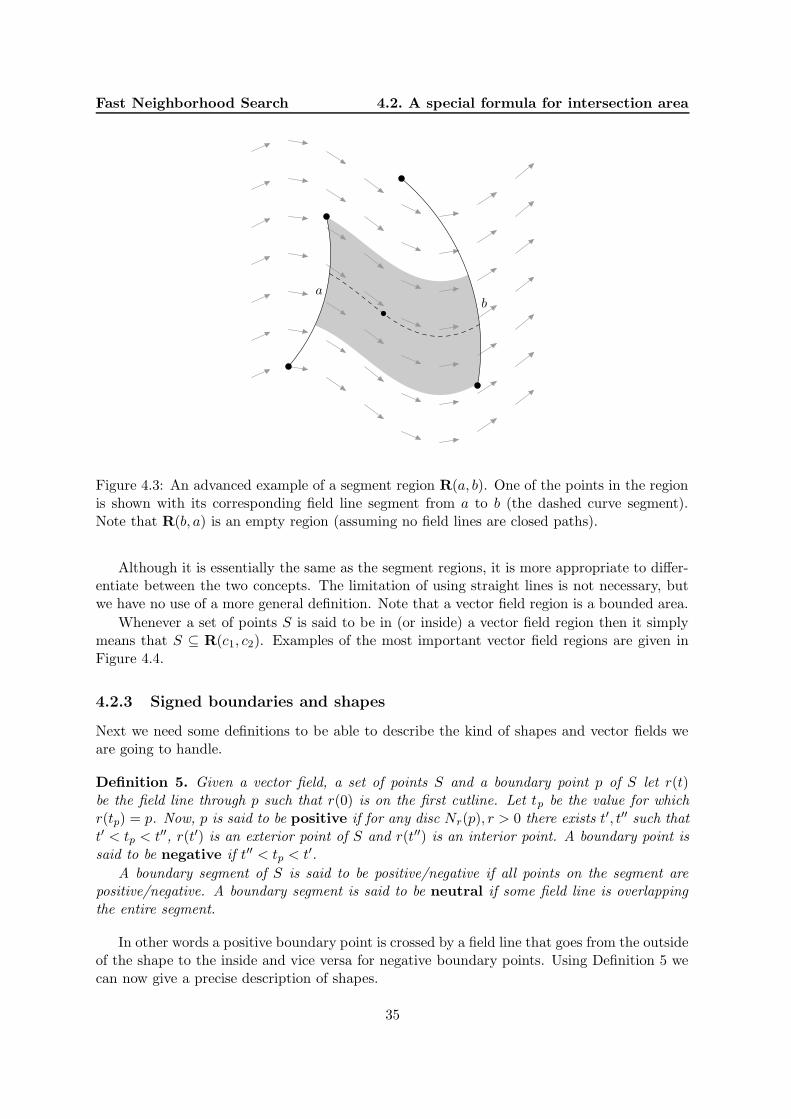
Fast Neighborhood Search 4.2. A special formula for intersection area
ab
Figure 4.3: An advanced example of a segment region R(a, b). One of the points in the regionis shown with its corresponding field line segment from a to b (the dashed curve segment).Note that R(b, a) is an empty region (assuming no field lines are closed paths).
Although it is essentially the same as the segment regions, it is more appropriate to differ-entiate between the two concepts. The limitation of using straight lines is not necessary, butwe have no use of a more general definition. Note that a vector field region is a bounded area.
Whenever a set of points S is said to be in (or inside) a vector field region then it simplymeans that S ⊆ R(c1, c2). Examples of the most important vector field regions are given inFigure 4.4.
4.2.3 Signed boundaries and shapes
Next we need some definitions to be able to describe the kind of shapes and vector fields weare going to handle.
Definition 5. Given a vector field, a set of points S and a boundary point p of S let r(t)be the field line through p such that r(0) is on the first cutline. Let tp be the value for whichr(tp) = p. Now, p is said to be positive if for any disc Nr(p), r > 0 there exists t′, t′′ such thatt′ < tp < t′′, r(t′) is an exterior point of S and r(t′′) is an interior point. A boundary point issaid to be negative if t′′ < tp < t′.
A boundary segment of S is said to be positive/negative if all points on the segment arepositive/negative. A boundary segment is said to be neutral if some field line is overlappingthe entire segment.
In other words a positive boundary point is crossed by a field line that goes from the outsideof the shape to the inside and vice versa for negative boundary points. Using Definition 5 wecan now give a precise description of shapes.
35

4.2. A special formula for intersection area Fast Neighborhood Search
a b
Figure 4.4: Examples of vector field regions. a) A horizontal vector field region with two finitecut lines. b) A rotational vector field region, where the two cut lines are identical.
Definition 6. A shape S in a vector field is a set of points which adhere the followingconditions: For the boundary B of S there must exist a division into a finite set of boundarysegments b1, ..., bn, where
• each boundary segment can be categorized as being positive, negative or neutral,
• for any i, j ∈ {1, . . . , n}, i 6= j : bi ∩ bj = ∅ (no points are shared between segments)
• and b1 ∪ . . . ∪ bn = B (the segments cover the entire boundary).
Furthermore, all boundary points must be in contact with the interior i.e. for any p0 ∈ S andr > 0, Nr(p0) contains at least one point which is in S, and which is not a boundary point.
An example of a shape is given in Figure 4.5. A shape does not have to be connected orwithout holes and it cannot contain isolated line segments or points. Note that any singularpoint in a boundary can be categorized as a neutral boundary segment, but a shape cannothave an infinite number of them since the total number of boundary segments is required tobe finite.
Figure 4.5 includes an example of a field line. The following lemma concerns the behaviorof such field lines.
Lemma 1. Suppose S is a shape in a vector field region. For any field line in the region (fromfirst to second cutline), which does not include any neutral boundary points from the shape, thefollowing will be true:
• If the field line crosses the shape then it will happen in an alternating fashion, regardingpositive and negative boundary segments, starting with a positive boundary segment andending with a negative boundary segment. Whether the field line is inside the shapealternates in the same way starting outside the shape.
• The field line will cross an even number of boundary segments.
• If a point p ∈ S is on the field line then moving forwards from p the field line will crossone more negative boundary segment than positive boundary segments. Moving backwards
36

Fast Neighborhood Search 4.2. A special formula for intersection area
Figure 4.5: The above set of points constitutes a shape in a horizontal vector field. Thebold boundary segments are positive boundary segments and the other boundary segments arenegative with the exception of the endpoints which are neutral. The dashed line is an exampleof a field line. Note how it crosses the boundaries of the shape.
from p the field line will cross one more positive boundary segment than negative boundarysegments.
• If a point p /∈ S is on the field line then moving forwards or backwards from p the fieldline will cross an equal number of positive and negative boundary segments.
Proof. We are only proving the first statement since the others follow easily.
Initially (at the first cut line) the field line is outside S. From the definition of positive andnegative boundary segments it is easy to see that when moving forwards on the field line thefirst boundary segment must be positive. It also follows from the definitions that the field linethen continues inside S and the next boundary segment must then be negative. This continuesin an alternating fashion ending with a negative boundary segment — otherwise S would notbe within the vector field region.
4.2.4 The Intersection Theorem
Now, we are getting closer to the main theorem. The next definition specifies a relation betweena point and a segment region which simply states whether the point is inside or outside theregion.
Definition 7. Given boundary segments a and b and a point p in a vector field region, wedefine the containment function as
C(a, b, p) =
{
1 if p ∈ R(a, b),
0 if p /∈ R(a, b).
This can be generalized to sets of boundary segments A and B:
C(A,B, p) =∑
a∈A, b∈B
C(a, b, p).
37

4.2. A special formula for intersection area Fast Neighborhood Search
Using the containment function and the following explicit division of boundary segmentsin positive and negative sets, we are now ready to present an essential theorem.
Definition 8. Given a shape S, we denote a finite set of boundary segments (as required bythe definition of a shape) Sb. We also denote the sets of positive and negative segments asS+
b = {b ∈ Sb | b is positive}, S−
b = {b ∈ Sb | b is negative}.
Theorem 2 (Containment Theorem). Suppose we are given a pair of shapes S and T anda point p in a vector field region, and that the field line of the point p does not contain anyneutral boundary points from the shapes, then the following is true:
p ∈ S ∩ T ⇒ w(p) = 1
p /∈ S ∩ T ⇒ w(p) = 0,
where
w(p) = C(T +b , S−
b , p) + C(T−
b , S+b , p)−C(T +
b , S+b , p)−C(T−
b , S−
b , p) (4.1)
Proof. In the following, whenever the terms forwards and backwards are used it means to startat p and then move forwards and backwards on the field line which goes through p.
From the definition of segment regions, it easily follows that the only pairs of boundarysegments affecting w(p) are those which intersect the field line going through p. Furthermore,the sum above is only affected by boundary segments from T found when moving backwardsand boundary segments from S found when moving forwards.
Assume that s positive boundary segments from S are crossed when moving forwards andt negative boundary segments from T are crossed when moving backwards. Now, by usingLemma 1 we can quite easily do the proof by simply counting.
First, assume that p ∈ S∩T . By definition p ∈ S and p ∈ T . It then follows from Lemma 1that s + 1 negative and t + 1 positive boundary segments are crossed when moving forwardsand backwards, respectively. Inserting this in equation 4.1 and doing the math reveals
w(p) = (t + 1)(s + 1) + ts− (t + 1)s− t(s + 1)
= ts + t + s + 1 + ts− ts− s− ts− t
= 1.
Now assume that p /∈ P ∩Q. There are three special cases, which can all be handled in avery similar way. In short,
p /∈ S ∧ p /∈ T : ts + ts− ts− ts = 0,p ∈ S ∧ p /∈ T : t(s + 1)− ts + ts− t(s + 1) = 0,p /∈ S ∧ p ∈ T : (t + 1)s− ts + (t + 1)s− ts = 0.
Definition 9. Given boundary segments a and b, let the area of a region R(a, b) be defined asA(a, b). We extend this definition to two sets of boundary segments A and B as follows:
A(A,B) =∑
a∈A, b∈B
A(a, b)
38
Fast Neighborhood Search 4.2. A special formula for intersection area
Standard calculus gives us that since R(a, b) is a bounded area then we have,
A(a, b) =
∫ ∫
R(a,b)1dA =
∫ ∫
p∈R2
C(a, b, p))dA.
We can now easily state and proof the main theorem.
Theorem 3 (Intersection Theorem). In a vector field region the intersection area α of twoshapes S and T can be calculated as:
α = A(T +b , S−
b ) + A(T−
b , S+b )−A(T +
b , S+b )−A(T−
b , S−
b )
Proof. Disregarding a finite number of field lines, we know that w(p) = 1 if p ∈ S ∩ T andw(p) = 0 otherwise. The finite number of field lines do not contribute with any area, so α canbe calculated as:
α =
∫ ∫
p∈R2
w(p)dA.
Using equation 4.1 and the fact that the integral of a sum is the same as the sum of integrals,
∫ ∫
R2
w(p)dA =
∫ ∫
p∈R2
C(T+b , S−
b , p)dA +
∫ ∫
p∈R2
C(T−
b , S+b , p)dA
−
∫ ∫
p∈R2
C(T+b , S+
b , p)dA−
∫ ∫
p∈R2
C(T−
b , S−
b , p)dA
Let us only consider∫ ∫
p∈R2 C(T+b , S−
b , p)dA which can be rewritten,
∫ ∫
p∈R2
C(T+b , S−
b , p)dA =
∫ ∫
p∈R2
∑
a∈T+
b, b∈S−
b
C(a, b, p)
=∑
a∈T+
b, b∈S−
b
∫ ∫
p∈R2
C(a, b, p)
=∑
a∈T+
b, b∈S−
b
A(a, b)
= A(T+b , S−
b ).
Rewriting the other three integrals we achieve the desired result.
The Intersection Theorem gives us a special way of calculating intersection areas, which weare going to see an example of in the next section. Note that it can also be used to calculatethe area of a single shape S by letting the “shape” T be a half space placed appropriately suchthat S is entirely inside T . This brings the Intersection Theorem very close to known formulasfor area computations.
39

4.2. A special formula for intersection area Fast Neighborhood Search
a
b
a
g
h
b
b
a
g
g′
h
c
b
a
Figure 4.6: The area A(a, b) can be in three different states. a) An empty region. b) A
triangular area, A(a, b) = hg2 . c) A trapezoidal area, A(a, b) = h(g+g′)
2 .
4.2.5 A simple example
It is time to make some practical use of the theoretical results. We are going to take a closerlook at the horizontal vector field and to simplify calculations we are going to limit the shapesto be polygons (holes are allowed). An edge excluding endpoints from a polygon is always astrictly positive, negative or neutral boundary segment no matter where it is placed in thehorizontal vector field and it is therefore natural to let the set of edges be the set of boundarysegments (endpoints are neutral boundary segments). Note that this is most often not aminimal set.
The basic calculation needed to use Theorem 3 is the area between two line segments.Formally, we are given two line segments a and b and we are interested in finding A(a, b)i.e. the area of the region between a and b. The first observation to make is that if the verticalextents of the two line segments do not overlap then the region is always empty. If the verticalextents do overlap then the region can be in three basically different states. The two lines canintersect, a can be to the left of b or a can be to the right of b. Examples of all of these threecases are given in Figure 4.6.
Finding A(a, b) is easy when a is to the right of b since this makes the region empty. Theother areas are not much harder. Intersecting segments reveal a triangular area and when a isto the left of b a trapezoidal area needs to be found.
We can now give an example of how to use Theorem 3. In Figure 4.7 all regions involvedin the calculation of the intersection of two polygons is given. The example uses polygonsand a simple horizontal vector field, but other shapes could easily be allowed as long as one isable to calculate the area of the regions. The same goes for the vector field.
Also note that if an edge from S does not have anything from T on its left side then it isnot involved in any regions used for the intersection calculation. This can hardly be a surprise,but it is exactly this asymmetry of the Intersection Theorem which will be utilized in the nextsection.
40

Fast Neighborhood Search 4.2. A special formula for intersection area
T
S
R(T+
b, S−
b)
T
S
R(T−
b, S+
b)
T
S
R(T+
b, S+
b)
T
S
R(T−
b, S−
b)
Figure 4.7: The above regions can be used to find the area of the intersection of the twopolygons S and T . The bold edges are the edges involved in the specified sets. The shadedareas in the top row contribute positively and the shaded areas in the bottom row contributenegatively. Area = A(T +
b , S−
b ) + A(T−
b , S+b )−A(T +
b , S+b )−A(T−
b , S−
b ).
41

4.3. Transformation algorithms Fast Neighborhood Search
4.3 Transformation algorithms
For some vector fields the calculation of intersection areas as given by the Intersection Theoremhas a much more interesting property. To see this we first need yet another definition and asmall lemma.
Definition 10. Given a shape S in a vector field region and a time value t we define thetransformation S(t) to be the shape obtained by moving all points of S along their correspondingfield lines with the given time value.
This is not as cryptic as it might seem. In the horizontal vector field this is a simplehorizontal translation and in the rotational vector field this is a rotation of S around thecenter of the vector field. Now we need a simple but essential lemma about the behavior ofboundary segments under a transformation.
Lemma 2. A boundary segment b in a shape S will not change type (positive, negative orneutral) when S is transformed by some value t.
Proof. This follows directly from the definition of the sign of boundary points (Definition 5).Assume that b is a positive boundary segment and let p0 be a point on b. We then know thatfor an arbitrarily small disc Nr(p0) there exists at least one exterior point p′0 and at least oneinterior point p′′0 in the disc such that both points are on the field line and p′0 is before p′′0.
When S is transformed the point p0 will be moved to pt. To show that pt is still a pos-itive boundary point we need to show that an arbitrarily small disc Nr(pt) contains at leastone exterior point and at least one interior point such that both points are on the field lineand the exterior point comes before the interior point. This is clearly obtained by using thetransformation of the points from a disc sufficiently small at p0 i.e. p′t and p′′t
The immediate consequence of this lemma is that the sets S+b and S−
b are unchanged whenS is transformed. This means that when calculating intersection areas between a shape T andS(t) for any value t then it is the same pairs of boundary segments that are involved in thecalculation. This is an advantage if one wants to find intersection areas for a set of values of t.
Unfortunately there is a problem with transformations of S in most vector fields. The formand the size of the shape is not preserved i.e. the distance between any pair of points in theshape is not the same before and after a transformation. In the following we are going to focuson vector fields that do preserve the shape.
Definition 11. A shape-preserving vector field is a vector field in which any transformationpreserves the distance between any two points.
Within the above type of vector fields, we can make a simple algorithm for two shapes Sand T which finds a good transformation of S with respect to having small overlap with T(Algorithm 3).
A small example of this algorithm is given in Figure 4.8. The example shows two trianglesS and T in a horizontal vector field. There are 8 breakpoints and the algorithm transformsS to each of these breakpoints to calculate the overlap with T . It turns out that a placementwith no overlap can be found.
If we assume that it takes linear time to find the boundary segments and that it takesconstant time to find the area of a region between two boundary segments then the runningtime of Algorithm 3 is as follows. Let n and m be the number of boundary segments in S and T ,
42

Fast Neighborhood Search 4.3. Transformation algorithms
Algorithm 3 Simple breakpoint method
Transform S such that S(0) is before T regarding field lines.Find sets of boundary segments Sb and Tb.Initialize an empty set of breakpoints B.for all a ∈ Sb do
for all b ∈ Tb doif R(a, b) is non-empty then
Find timing value t where a and b starts intersecting.Find timing value t′ where a and b stops intersecting.Save the timing values t and t′ as breakpoints in B.
end ifend for
end forInitialize the smallest overlap found, min = ∞.for all t ∈ B do
if S(t) is within the vector field region thenSet tmp = area of S(t) ∩ T (using the Intersection Theorem).if tmp < min then
Set min = tmp.end if
end ifend forReturn min.
S T
a
ST
b
Figure 4.8: A small example of how the horizontal placement of S is found in relation to Twithin the boundaries of a vector field region (the box) using Algorithm 3. The algorithmwill find 8 breakpoints (the lengths of the double arrows). Translating S according to each ofthese breakpoints reveals a non-overlapping solution within the boundaries of the box (the lastbreakpoint).
43

4.3. Transformation algorithms Fast Neighborhood Search
Figure 4.9: The horizontal position of the triangle above does not correspond to any break-point. The area of overlap is clearly increased if the triangle is shifted left or right. ThereforeAlgorithm 3 cannot find the optimal horizontal translation of the triangle (which is to leave itwhere it is).
respectively, then there are O(nm) checks for breakpoints which produce at most k = O(nm)breakpoints. For each of these breakpoints the calculation of overlap can be done in O(k) time(only the segment pairs which also cause breakpoints need to be considered to contribute tothe overlap). This reveals a total running time of O(nm + k2) or O(n2m2) in the worst case.
Finding the overlap at a single breakpoint is worst case O(nm) which is also a lower limitfor the worst case of the problem of finding the intersection area of two polygons.
The algorithm does not necessarily find the best placement of S since this is sometimesbetween two breakpoints. An example of such a situation is given in Figure 4.9. But thealgorithm still has a very nice property as the following lemma shows.
Lemma 3. Suppose we are given a vector field region in which two shapes S and T are placed.If there exists a transformation of S, where S does not overlap T then either Algorithm 3 willfind it or it is located where S touches a limit of the vector field region.
Proof. Assume we are given a placement of S which does not overlap with T and which doesnot correspond to a breakpoint as found in Algorithm 3. Then it is clearly possible to eithermove S until it touches T , which corresponds to a breakpoint, or until it touches a limit of thevector field region. In both cases no overlap is involved and the algorithm would have triedthe placement as one of the breakpoints. This contradicts the initial assumption.
The running time of Algorithm 3 is quite good when compared to a standard overlapalgorithm which could also be used at each breakpoint. An efficient implementation might runrun in O((n + m) log(n + m)) on an average basis (worst case is still O(nm)) resulting in arunning time of O(k(n+m) log(n+m)) if k breakpoints are found. Assuming k is in the orderof O(n + m) this is a running time of O((n2 + m2) log(n + m)). Algorithm 3 can handle it inO(n2 + m2).
But in some cases we can make an even smarter algorithm. It depends on whether wecan express how the area of a given segment region grows with respect to the transformationtime t. In a horizontal vector field this reveals an algorithm which is faster than Algorithm 3and which is guaranteed to find a minimum (Section 4.4). First we are going to present thealgorithm in a more general setting as seen in Algorithm 4.
44

Fast Neighborhood Search 4.3. Transformation algorithms
Algorithm 4 Iterative breakpoint method
Transform S such that S(0) is before T regarding field lines.Find sets of boundary segments Sb and Tb.Initialize an empty set of breakpoints B.for all a ∈ Sb do
for all b ∈ Tb doif R(a, b) is non-empty then
Find timing value t where a and b starts intersecting.Find timing value t′ where a and b stops intersecting.Mark the breakpoints as primary and secondary breakpoints respectively.Save the timing values t and t′ as breakpoints in B.
end ifend for
end forSort the breakpoints in B in ascending order.Initialize the smallest overlap found, min = ∞.Initialize an intersection area function, Int(x) = 0.for all t ∈ B do
if t is a primary breakpoint thenA new segment region is “growing”. Find a function A(x) which reflects this.
else if t is a secondary breakpoint thenAn existing segment region is “changing”. Find a function A(x) which reflects this.
end ifSet Int(x) = Int(x) + A(x).Set tmp = the minimum of Int(x) in [t, t′], where t′ is the next breakpoint.(disregarding special cases e.g. to ensure that S is inside the vector field region)if tmp < min then
Set min = tmp.end if
end forReturn min.
45

4.4. Translation of polygons Fast Neighborhood Search
There are three major stages in this algorithm: Collecting breakpoints, sorting breakpointsand iterating breakpoints. In the first stage the breakpoints are explicitly marked as eitherprimary or secondary. This can be useful information in the third stage, where the essenceof this algorithm lies. Unlike Algorithm 3 the breakpoints are sorted in the second stage. Bydoing this the third stage becomes surprisingly easy. It turns out that we no longer need touse the Intersection Theorem repeatedly. This is due to the fact that the involved pairs ofboundary segments at time t1 is a subset of the involved pairs of boundary segments at timet2 if t2 > t1.
Note that for some boundary segments it might be convenient/necessary to introduce extrabreakpoints between the primary and secondary breakpoints to be able to make more changesto the area function. But in the following we are going to assume that two are enough.
Algorithm 4 finds the transformation of S that results in the smallest possible intersectionarea with T . The efficiency of the algorithm depends on how well segment region functionscan be added and how easy it is to find the minimum of the resulting function within a giveninterval. Detailed examples are presented in the following sections.
Now there is one final general observation to do.
Lemma 4. There exists only two classes of two-dimensional shape-preserving vector fields(and regions): Rotational and translational vector fields.
Proof. This follows directly from a known fact in Euclidean geometry, in which there onlyexists three kinds of shape-preserving transformations: Rotation, translation and reflection.We have already seen the vector fields related to rotation and translation. It is not possibleto construct a vector field which matches reflection. This is intuitively clear since reflectionrequires one to lift the shape and turn it around which clearly requires the freedom of threedimensions to maintain the shape in the process.
It is not unlikely that non-shape-preserving vector fields could be useful, but they are notconsidered any further in this thesis.
4.4 Translation of polygons
We have already seen how to calculate the intersection area of two polygons in a horizontalvector field. The only thing left to be able to use Algorithm 3 is to find the breakpointsand this is a simple matter. Therefore we already have an algorithm which is able to findnon-overlapping solutions to the translation of a given polygon (if they exist).
To be able to use Algorithm 4 we need to do some additional calculations. Finding thebreakpoints is no different than before and sorting them is no problem. The new part is thatwe need to find functions that tell us how the area of a region changes with translation. InFigure 4.10 the various stages of a segment region are illustrated. It also shows the placement ofthe segments at the primary and secondary breakpoints as they are described in the algorithm.Between the primary and the secondary breakpoint the segment region is a triangular area(Figure 4.10b). After the secondary breakpoint it changes to a trapezoidal area. We have seenthese areas earlier, but this time we need to describe the areas with respect to the time of thetranslation.
The area of the trapezoid is very easy to describe. It is simply the area of the triangle inFigure 4.10c plus a simple linear expression based on the height of the trapezoid. Using the
46

Fast Neighborhood Search 4.4. Translation of polygons
a
b
a
t′
h′
b
b
a
c
h
c
b
a
t′′
h
d
b
a
Figure 4.10: a) The segment region is empty until the primary breakpoint. b) The areais growing quadratically between the breakpoints. c) At the secondary breakpoint the areagrowth changes... d) to grow linearly.
variables shown in the figure,
As(t′′) = ht′′ +
hc
2,
where As is the area of the segment region after the secondary breakpoint.The triangle is a bit harder. The important observation is that the height h ′ of a triangle
must be hct′. Then it easily follows that
Ap(t′) =
h′t′
2=
h
2c(t′)2,
where Ap is the area of the segment region between the primary and the secondary breakpoint.Now the above functions depend on translation values t′ and t′′ which are conveniently
zero at the primary and secondary breakpoints respectively. To add such functions we needto formulate them using the same translation offset value t. If we let tp, ts be the translationdistances to the involved primary and secondary breakpoints (the breakpoint time values inthe algorithm) then we can do this by simply letting t′ = t − tp and t′′ = t − ts in the aboveformulas. This reveals the following two formulas for triangles and trapezoids respectively,
Ap(t) =h
2c(t− tp)
2 =h
2c(t2 − 2tpt + t2p) =
h
2ct2 −
htpc
t +ht2p2c
,
As(t) = h(t− ts) +hc
2= ht− hts +
hc
2.
These functions can be added such that the result is never worse than a quadratic function forwhich we can easily find a minimum.
Now, imagine we are translating a polygon P over a polygon Q to find an optimal placement(minimum overlap). Finding the breakpoints is easy and can be done with a few comparisonsand calculations for each pair of edges (one from P and one from Q). Assume there is nedges in P and m edges in Q. Finding the breakpoints then takes time O(nm). In the worstcase breakpoints are produces by all pairs of edges giving us k = O(nm) breakpoints. Sortingthe breakpoints takes time O(k log k). Constant work is done at each breakpoint (adding afunction and finding a minimum) and therefore the total running time will be O(nm+k log k).
47

4.5. Rotation of polygons Fast Neighborhood Search
c
No rotation
c
An optimal rotation
Figure 4.11: A simple example of a rotation yielding a placement with no overlap.
Although the above calculations are based on a horizontal translation, an algorithm forvertical translation easily follows. Using appropriate area calculations it is possible to do thetranslation in any direction. More generally it is only the area calculations that is the reasonto restrict the shapes to be polygons. Algorithms could easily be made to translate othershapes e.g. circles, but it might not be possible to add the area functions in an efficient waythereby complicating the calculation of overlap at a breakpoint and especially the search for aminimum. This problem is also one of the main concerns in the following section.
4.5 Rotation of polygons
We have efficiently solved the problem of finding an optimal translation of a polygon. A verysimilar problem is to find the optimal rotation of a polygon i.e. how much is a polygon to berotated to get the smallest possible overlap with all of the other polygons. A simple exampleis given in Figure 4.11.
This problem corresponds to the rotational vector field and is basically no different thantranslation apart from the area calculations. Unfortunately there are a couple of extra issueswhich need to be handled.
First of all the edges of a polygon cannot be directly adopted as boundary segments sincesome edges can have both positive and negative parts. These edges are quite easy to identifyand they can always be split into two parts. This is illustrated in Figure 4.12. Note thatneutral boundary segments are always singular points since a straight line can never overlap afield line.
Another problem is that the cut line(s) can rarely be placed without cutting some polygons(especially the one to be rotated). These shapes will then violate the condition of all shapesbeing inside the vector field region. It turns out that this problem is not easily handled. Inthe following, we simply assume that the cut line is placed as was shown earlier in Figure 4.4band that no shapes crosses this line. In practice a simple solution is to cut all polygons intotwo parts at the cut line, but obviously this is not very efficient.
Polygons are normally given in Cartesian coordinates, but in the following context it willbe much easier to work with polar coordinates. The center for these coordinates are natu-
48

Fast Neighborhood Search 4.5. Rotation of polygons
Figure 4.12: If an edge passes the center of rotation perpendicularly then it must be split intotwo parts. This is to ensure that all edges are positive, negative or neutral. The bold linesabove are the positive boundary segments and the dashed lines show where it is necessary tosplit lines.
49

4.5. Rotation of polygons Fast Neighborhood Search
ab
ab
ab a
b
Figure 4.13: A segment region goes through 3 stages. 1. No overlap. 2. An almost triangulararea (see the formula in the text). 3. A concentric trapezoid.
rally placed at the center of the rotation i.e. the center of the polygon to be rotated. Thesecoordinates can be precalculated for the polygon to be rotated, but unfortunately they needto be calculated for all other involved polygons. Given Cartesian coordinates (x, y) the polarcoordinates (r, θ) are given by,
r =√
x2 + y2, tan θ =y
x.
Just like translation a segment region R(a, b) between two boundary segments, a and b,goes through three different stages. These stages are illustrated in Figure 4.13 and 4.14.These figures also show that there are two basic variations of the area between two segmentsdepending on how the segments meet.
An implementation of the simple breakpoint algorithm (Algorithm 3) is now straightfor-ward. Finding the breakpoints is a question of calculating intersections between circles andsegments and area calculations does not involve much more than an intersection calculationbetween boundary segments.
Now the big question is whether or not we can make an iterative algorithm as we could forthe translational problem. To do this we first need to find functions expressing the area of thesegment regions.
Area calculation is almost the same for the two basic variations. In both cases we needto calculate the area of a circle segment1 and a triangle. This is illustrated in Figure 4.15and 4.16. In the following we refer to the variables used in these illustrations. The easy partto calculate is the area of the circle segment, which is simply
As(θ) =1
2r2(θ − sin θ).
1Given two points on a circle the circle segment is the area between the circle arc and the chord between thetwo points.
50

Fast Neighborhood Search 4.5. Rotation of polygons
a
b
ab
ab a
b
Figure 4.14: The area between line segments have two basic variations. In the above examplethe line segments meet first closest to the center. In Figure 4.13 it was the opposite. Note thatthe areas which need to be calculated have different shapes.
θ
αα′
γγ′
rr
p
q
Figure 4.15: Variation 1 of the area between intersecting boundary segments.
51

4.5. Rotation of polygons Fast Neighborhood Search
θ
α α′
γ γ′
rr
p
q
Figure 4.16: Variation 2 of the area between intersecting boundary segments.
The pq-triangles in the figures are a bit more difficult. Let x = π−θ2 which is the angle at
the dashed corners on the figures.Now we need γ and γ ′ shown on the figures and they can be calculated in the following
way for both variations,γ = |x− α|,γ′ = |x− α′|,
Using the variables above and the sine relations the following expressions can be deduced,
p = 2r sinθ
2,
q = psin γ′
sin(γ + γ′),
At(θ) = pq sin γ.
Now the area between boundary segments for variation 1 is At(θ)+As(θ) and for variation 2it is almost the same, At(θ)−As(θ). When the segments no longer intersect then a constant canbe calculated e.g. by using the above formulas and then a linear expression must be added. Ifθ is the rotation since the second breakpoint and r1 and r2 are the radii to the two breakpoints(r2 < r1) then it can be expressed as
A(θ) =1
2(r2
1 − r22)θ.
The functions needed to describe these areas vary a lot in complexity and this affects therunning time of a rotational variant of Algorithm 4. The functions are not easily added withthe exception of the linear expressions and finding the minimum between two breakpoints isfar from trivial. We are not going to pursue this subject any further in this thesis.
52

Chapter 5
Miscellaneous Constraints
5.1 Overview
Until now we have shown how to handle a quite general nesting problem allowing free trans-lation, rotation and flipping. As mentioned in Chapter 2 there can be a multitude of extraconstraints for an industrial nesting problem depending on the industry in question. We be-lieve that our solution method can handle many of these constraints without a lot of hassle.To substantiate this claim this chapter will present and discuss various constraints. For mostof them this includes a description of how to incorporate them to be handled by our solutionmethod. Some of them will also be part of our implementation.
Note that the majority of solution methods in the existing literature can only handle fewof the following constraints. And more importantly, it is most often very unclear how they canbe adapted to allow more constraints. This is especially true for the legal placement methods.
Also note that not all of the following are constraints in a strict sense. Some are betterdescribed as variants of the nesting problem which require special handling.
• Stencil shapes.The shapes of the stencils are never a problem. Any shape can be approximated witha polygon which we are able to handle. It can also have holes since this is clearly noproblem for the translation and rotation algorithms.
Note that it could be advantageous to preprocess holes in polygons filling them as denselyas possible. This could be stated as a knapsack problem and would afterwards make theremaining problem easier.
• Fixed positions.Sometimes it is convenient to fix the position of a stencil. This is no problem for GLSsince the offsets of the stencil can be set to the desired position and then never changedagain while still including the stencils in any overlap calculations with other stencils.
• Material shape.In some cases the material needs to have an irregular shape. Combining the two firstconstraints this turns out to be an easy problem. Simply make a stencil correspondingto a hole and fix its position.
• Correspondence between stencils.In the textile industry the garment could have some kind of pattern. To allow this
53

5.1. Overview Miscellaneous Constraints
a b
Figure 5.1: Examples of patterns and stencils requiring special attention due to pattern re-quirements. a) The two shapes can be freely translated vertically, but horizontally they haveto follow each other if their patterns are supposed to be the same. b) If the shape needs tohave the pattern in a certain way then it can only be translated to positions where the patternis repeated.
pattern to continue across a seam it might be necessary to fix two or more stencils toalways being moved the same amount horizontally and/or vertically. It might even benecessary to rotate them by the same amount. An example is given in Figure 5.1a.
For our solution method this is simply a question of involving more stencils in the trans-lation/rotation algorithms.
• Pattern symmetries.In some cases, the placement options of stencils might be limited to some fixed set. Thereason could (again) be patterns in a garment and the desire to get specific patternsymmetries or pattern continuations at seams.
It is no problem for our translation algorithm to handle this. Just avoid finding the trueminimum and instead find the minimum among the legal set of translations. This cane.g. be done by introducing special breakpoints corresponding to the distances for whichoverlap calculations must be done. Intervals could also be handled if necessary.
• Limited rotation angles.Some nesting problems might only allow a fixed set of rotation angles. This is most oftenthe case in the textile industry since most kinds of fabric have a grain. Though oftensome level of “fine tuning” is allowed i.e. a rotation within e.g. [−3◦, 3◦].
No matter what sets or intervals of rotation angles are allowed it is no problem to handlein the rotation algorithm.
• Quality areas.In some cases, material and stencils can be divided into regions of different quality andquality requirements (respectively) with the purpose that a legal placement adheres allquality requirements. An example and a surprisingly easy way to handle this can befound below in Section 5.2.
• Margins between polygons.Some cutting technologies require a certain distance between all stencils. This seems tobe a quite easy constraint since polygons can simply be enlarged by half the required
54

Miscellaneous Constraints 5.1. Overview
distance, but it turns out that there is a few pitfalls. This is described and handled inSection 5.3.
• Folding.Now, imagine a sheet of fabric which is folded once. Some symmetric stencils can beplaced at the folding such that only half of it is visible on the upper side i.e. only halfof it is involved in the nesting given that it is placed somewhere along the folding. Insome cases this might allow better solutions to be found. It is also possible to allownon-symmetric stencils to be placed at the folding, but it will invalidate other areas ofthe fabric and it will complicate the cutting process.
Our algorithm easily allows a stencil to only being allowed to be moved along the folding,but the difficulty lies in deciding when it is profitable to do so. We are not going to handlethis constraint.
• Stencil variants.In the textile industry some stencils can be allowed to be divided into two (or more)parts since they can be stitched together at a later stage. Naturally they fit very welltogether so it might not be an advantage to split them since it also makes the problemharder (more stencils).
This is also very close to the concept of meta stencils suggested by various authors [4, 1]i.e. the pairing of stencils to reduce the complexity of the problem. Dynamic pairingand splitting of stencils is probably an improvement to most solution methods, but thestrategies for finding good pairings are not trivial. We are not going to discuss it anyfurther in this thesis.
The final couple of items in this list is not really constraints. They are variations of thenesting problem, which are both interesting and very relevant in some industrial settings.
• Repeated pattern nesting.This variant of strip packing was mentioned in Chapter 2. We are now ready to discussit in more detail in relation to our solution methods. Repeated pattern nesting allowsstencils to wrap around the edges of the material. The reasoning for allowing this isthat sometimes one needs to nest a few stencils which is then going to be cut repeatedlyfrom a long strip of material. An example is given in Figure 5.2. Note that the heightis fixed in the example. One could also allow the pattern to repeat both vertically andhorizontally.
It is surprisingly “easy” to alter our solution method to allow repeated patterns. Trans-lation becomes similar to rotation in the general case since rotation already works with arepeated pattern. If the material is wrapped around a cylinder this becomes even moreevident. Minor issues must also be handled e.g. to handle rotation, but there are noserious problems with the repeated pattern variation of strip packing. Not even if onewants to do it both horizontally and vertically.
• Minimizing cutting path length. When an efficient nesting has been found and it is readyfor use, another interesting problem turns up. The stencils now need to be cut out of thematerial, which can happen in different ways depending on the material and the cuttingtechnology. Metal can in some cases be punched out of the material, but often some kind
55

5.2. Quality areas Miscellaneous Constraints
Pattern width
Figure 5.2: An example of repeated pattern nesting in 1 dimension. The pattern width is tobe minimized, but unlike strip packing the stencils can wrap around the vertical limits.
of laser, water or plasma cutter is used. Other technologies apply in the textile industry,but most often there is a need for a cutting path. To save time it is important that thecutting path is as short as possible.
The length of the cutting path depends on the placement found in the nesting process.One of the original goals of this thesis was to examine whether the minimization ofthe cutting path length could be integrated with the nesting algorithm. This goal wasdiscarded in favor of 3D nesting, but in Section 5.4 we describe an algorithm to simplyfind the shortest cutting path for a given placement.
5.2 Quality areas
The leather nesting industry poses one of the most interesting constraints. Imagine that weare going to make a leather sofa and that we are given an animal hide so that we can cut outthe needed parts. The animal hide is of varying quality and we need to make sure that thegood areas of the hide are used in the most demanding areas of the sofa.
Now assume that the animal hide can be divided into a number of areas which correspondto different quality levels Q1, ..., Qn. Assume that Q1 is the best quality. If we divide thestencils into areas of minimum required quality levels then we can formulate the problem weneed to solve: Pack the stencils within the material (the animal hide) so that no stencils overlapand so that the quality requirement Qi of any part of any stencil is the same or worse than thequality of the material Qj i.e. i ≥ j. An example of a piece of material with different levels ofquality is given in Figure 5.3.
Although this seems like a complicated problem, it can actually be solved with the help ofthe constraints already described by doing the following.
• Divide each stencil into a set of stencils corresponding to each quality area. Fix theinterrelationship of these stencils i.e. when one is moved/rotated then the others follow(they should have a common center for rotation).
• Add a stencil with fixed position corresponding to each quality area of the material.
• Alter the transformation algorithms to only include segment pairs which violate thequality requirements.
56

Miscellaneous Constraints 5.3. Margins between polygons
Q1
Q2
Q3
Q4
Figure 5.3: A piece of material, e.g. an animal hide, can have areas with different levels ofquality. The stencils to be placed can have different quality requirements — even a singlestencil can be divided into areas with specific quality requirements.
5.3 Margins between polygons
Some cutting technologies require a certain distance between the stencils as illustrated inFigure 5.4a. In the following we will assert that the required distance between any pair ofpolygons is the same. This assertion is essential for all results in this section.
5.3.1 A straightforward solution
The obvious way to get around this requirement is to enlarge all stencils by adding a marginwhich has half the width of the required distance. This is e.g. suggested by Heckmann andLengauer [35] in an article focused on the textile industry, but they do not specify how to dothis in practice. They simply state that one should calculate an enclosure where all edges havea distance of at least half of the required distance from the edges of the original stencil.
Their illustration of such an enclosure seems to indicate that they do this as illustrated inFigure 5.4a. Each edge in the original stencil is translated half the required distance betweenstencils and these edges are then stretched/shortened to make the enclosure. It is quite easyto calculate the corner points of this enclosure, but it is also obvious that this enclosure isnot a perfect approach. This is emphasized in Figure 5.4b where two stencils are forced to befarther apart than necessary. The angle α determines how much farther. This is illustrated inFigure 5.5a where the distance x can be expressed as:
x = M
sin(α
2 ), 0 < α ≤ π
x = M
sin(α−π
2 ), π ≤ α < 2π
57

5.3. Margins between polygons Miscellaneous Constraints
α
a b
Figure 5.4: a) A simple enlargement of two polygons can guarantee some required minimaldistance between them. b) A simple enlargement can force polygons to be farther apart thannecessary
αα
2
x
Mα
a b
Figure 5.5: a) The distance x should be close to the distance M , but this is clearly not thecase. b) The problem can be solved by rounding the corners
58

Miscellaneous Constraints 5.3. Margins between polygons
The value M is the width of the added margin to the stencil and optimally x should havethe same value. Unfortunately x → ∞ when α → 0. The same is true for α → 2π, but thisis not the only problem with the latter formula since it is actually not correct. When α > π(concave corners) the length of the neighboring edges also need to be taken into account. Atthis point it only causes the enlargement to be bigger than necessary (not always), but laterit even causes too small enlargements. We will deal with it then and show a different way ofhandling the concave corners.
5.3.2 Rounding the corners
In the following we are focusing on the case of α < π. An optimal enclosure, i.e. an enclosurethat does not remove any configurations from the set of legal solutions, must have rounded cor-ners as illustrated in Figure 5.5b. The rounding of a corner is simply a circular arc with radiusM . Unfortunately we only allow polygons and therefore we need to make some approximation.We have three objectives for this approximation.
• It must contain the optimal enclosure.
• It should be as small as possible.
• It should introduce as few new vertices as possible.
In other words, we need to maximize the effect of using extra vertices. If we only use 1vertex at a given corner then its optimal position will be as already shown in Figure 5.5a. Theangle at this new corner is identical to the angle α in the original stencil. When using morethan 1 vertex then we would like the new angles to be as large as possible. It turns out thatthis can be done quite easily as illustrated in Figure 5.6.
The span of the round corner is α′ = π−α and given V extra vertices we get x = α′
V. Now
due to the right angles it can easily be shown that all the new angles are π− x = π− α′
V. The
distance from the original corner point to each of the new corner points are the same and usingsine relations this can be expressed as M
sin( π−x
2).
5.3.3 Self intersections
The above approach works fine when observing a single corner point, but problems arise whenwe look at the entire polygon. The first problem is quite obvious. Some polygons when enlargedwill self intersect. This is a problem which can basically be solved in two ways. Either the selfintersections are removed or else they are ignored. If they are ignored then all other algorithmswill be required to work correctly with self intersecting polygons.
The second problem is a bit more subtle. When enlarging a polygon the rounded cornerof a convex corner can interfere with a concave corner in such a way that the polygon is notonly self intersecting — it also no longer contains the optimal enclosure. An example can beseen in Figure 5.7a. The problem is caused by the assumption that all of a rounded corner ispart of an optimal enclosure. The easiest way to avoid this problem is to add two vertices foreach concave corner as illustrated on Figure 5.7b. They are placed with a distance of M inperpendicular directions to the two neighboring edges.
Now an algorithm can round the convex corners freely, place two points for each concavecorner and finally remove the self intersections. Note that this algorithm is stated withoutproof of correctness.
59
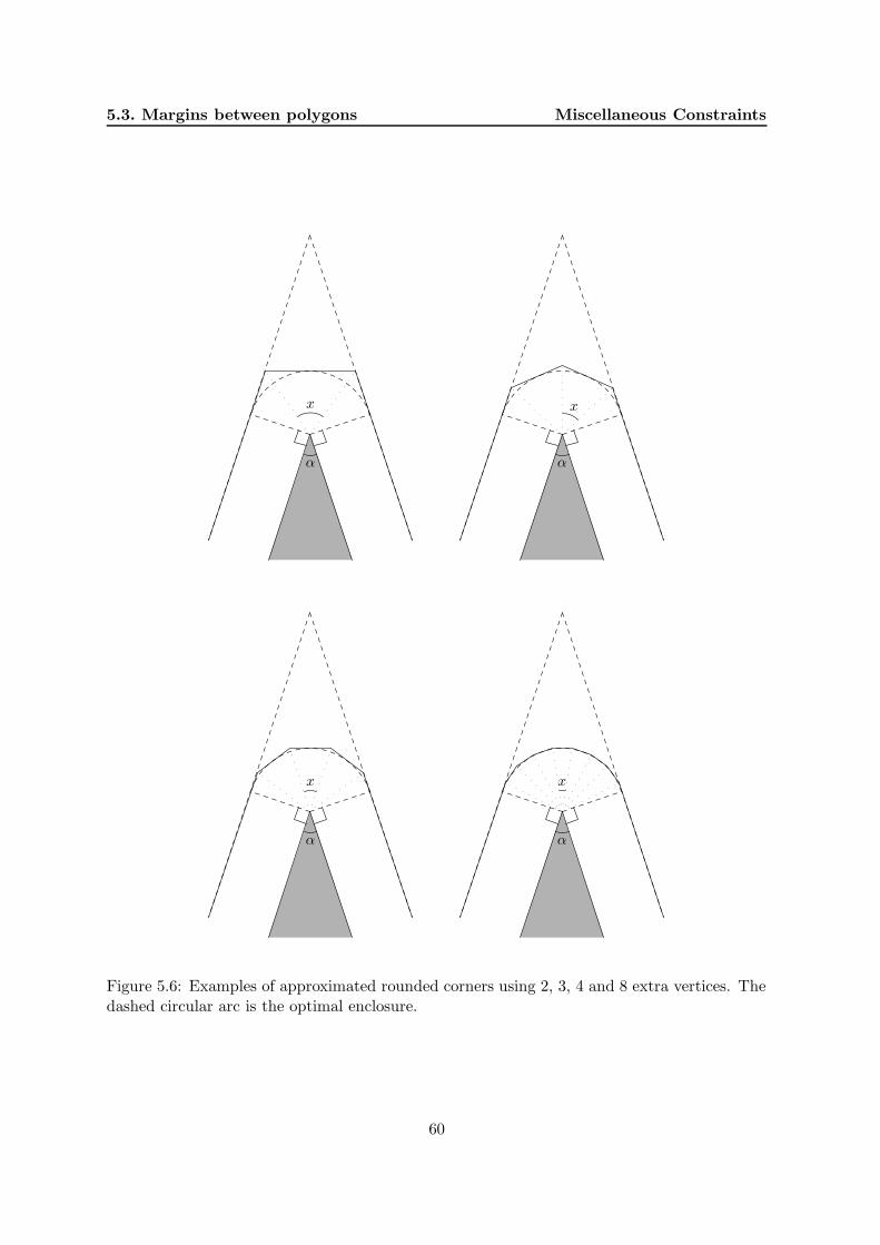
5.3. Margins between polygons Miscellaneous Constraints
x
α
x
α
x
α
x
α
Figure 5.6: Examples of approximated rounded corners using 2, 3, 4 and 8 extra vertices. Thedashed circular arc is the optimal enclosure.
60

Miscellaneous Constraints 5.4. Minimizing cutting path length
a b
Figure 5.7: a) A naive rounding of corners can cause the resulting polygon to be illegal in thesense that the margin is no longer guaranteed. b) A subtle fix to this problem is the additionof two points for each concave corner (and a removal of the self intersection.
5.4 Minimizing cutting path length
When given a legal placement the problem of finding a short or even the shortest cutting pathis a natural next step. In the following we will shortly describe how hard this problem is andhow it can be solved.
Clearly all line segments in a given placement p must be cut. Now let Gp be the graphcontaining all of the lines which need to be cut as edges and all endpoints of lines as nodes.Edge weights are the Euclidean distances. Some line segments can overlap and thereby onlyneed to be cut once. Assume that these have been combined in Gp such that all edges areunique. An example of this simple transformation is given in Figure 5.8a and b. Note that inpractice precision problems can make it difficult to find overlapping lines.
Now, assume that this graph is connected which it certainly will be if it is a good solutionto a nesting problem. A shortest cutting path might involve lines not present in this graph,but first we assume that the problem we need to solve is to find a path in this graph whichvisits all edges at least once. We would also like the path to end where it started although thismight not be important in some cases. This problem is known as the Chinese postman problem(CPP) and it can be solved in polynomial time as shown by Edmonds and Johnson [27]. Ifall nodes have even degrees then it is even easier. This is one of the oldest problems in graphtheory: Finding an Euler tour [30, 27], which is a very simple problem and a solution will onlyvisit each edge exactly once. Therefore nothing would be gained by introducing new edges.
Most often all nodes do not have even degrees which means that a shorter path mightbe found by introducing new edges in the graph corresponding to moving the cutting headwithout cutting.
If we assume the graph is connected then the extra edges can be reduced to the edges thatremains to make Gp a full graph. Any other edges would have to at least have one end on anexisting edge creating a node of degree 3. The degree of any node must be even in a solutionand therefore yet another edge must be connected to this node. Two non-cutting edges arenow connected to this node which means that they could just as well be connected directlyleaving the edge as it was.
61

5.4. Minimizing cutting path length Miscellaneous Constraints
a b c d
Figure 5.8: Various steps in the process of finding a shortest cutting path. a) A given nestingsolution. b) A graph corresponding to the edges which need to be cut. c) The odd nodes ofthe graph with all vertices connected. The thick lines show a minimal 1-matching. d) Theedges from the 1-matching is added to the original graph revealing a graph with even nodesonly. A solution is now easily found.
The problem we end up with is a full graph where a cyclic path has to be found whichmust include a connected subset of the graph. This problem is a restricted version of the rural(Chinese) postman problem (RPP) and this is in general an NP-hard problem [42], but if thesubgraph Gp is connected then the problem essentially reduces to CPP [29] i.e. it can be solvedin polynomial time using almost the same algorithm as for CPP [27] (actually the algorithmis even simpler because we are using a full graph with Euclidean distances). Four steps arenecessary:
1. Generate a new full graph Godd with the odd nodes from Gp (Figure 5.8c).
2. Find a minimum 1-matching of Godd (a 1-matching is a subset of edges of Godd such thateach node is connected to exactly one of these edges).
3. Add the edges from the 1-matching to the original graph Gp to make a new graph G′p
(Figure 5.8d).
4. Find an Euler tour in G′p.
The hardest step is the second step, but according to Cook and Rohe [15] a 100000 nodegeometric instance can be solved in about 3 minutes on a 200 MHz Pentium-Pro.
The following observations have also been made regarding the cutting path. If a placementconsists of highly irregular shapes which rarely share edges then the graph will have very fewodd nodes making the problem very easy. If the graph is disconnected (e.g. because of somemargin requirements for the solution) then not only is the problem NP-hard, the additionaledges are not necessarily between nodes either. Finally, in practice it might take time to switchthe cutting machine on and off making it more expensive to add non-cutting lines. It mightalso take extra time to turn at corners.
62
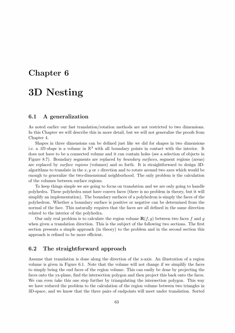
Chapter 6
3D Nesting
6.1 A generalization
As noted earlier our fast translation/rotation methods are not restricted to two dimensions.In this Chapter we will describe this in more detail, but we will not generalize the proofs fromChapter 4.
Shapes in three dimensions can be defined just like we did for shapes in two dimensionsi.e. a 3D-shape is a volume in R
3 with all boundary points in contact with the interior. Itdoes not have to be a connected volume and it can contain holes (see a selection of objects inFigure 8.7). Boundary segments are replaced by boundary surfaces, segment regions (areas)are replaced by surface regions (volumes) and so forth. It is straightforward to design 3D-algorithms to translate in the x, y or z direction and to rotate around two axes which would beenough to generalize the two-dimensional neighborhood. The only problem is the calculationof the volumes between surface regions.
To keep things simple we are going to focus on translation and we are only going to handlepolyhedra. These polyhedra must have convex faces (there is no problem in theory, but it willsimplify an implementation). The boundary surfaces of a polyhedron is simply the faces of thepolyhedron. Whether a boundary surface is positive or negative can be determined from thenormal of the face. This naturally requires that the faces are all defined in the same directionrelated to the interior of the polyhedra.
Our only real problem is to calculate the region volume R(f, g) between two faces f and gwhen given a translation direction. This is the subject of the following two sections. The firstsection presents a simple approach (in theory) to the problem and in the second section thisapproach is refined to be more efficient.
6.2 The straightforward approach
Assume that translation is done along the direction of the x-axis. An illustration of a regionvolume is given in Figure 6.1. Note that the volume will not change if we simplify the facesto simply being the end faces of the region volume. This can easily be done by projecting thefaces onto the yz-plane, find the intersection polygon and then project this back onto the faces.We can even take this one step further by triangulating the intersection polygon. This waywe have reduced the problem to the calculation of the region volume between two triangles in3D-space, and we know that the three pairs of endpoints will meet under translation. Sorted
63
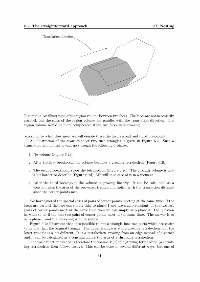
6.2. The straightforward approach 3D Nesting
Translation direction
Figure 6.1: An illustration of the region volume between two faces. The faces are not necessarilyparallel, but the sides of the region volume are parallel with the translation direction. Theregion volume would be more complicated if the two faces were crossing.
according to when they meet we will denote these the first, second and third breakpoint.
An illustration of the translation of two such triangles is given in Figure 6.2. Such atranslation will almost always go through the following 4 phases.
1. No volume (Figure 6.2a).
2. After the first breakpoint the volume becomes a growing tetrahedron (Figure 6.2b).
3. The second breakpoint stops the tetrahedron (Figure 6.2c). The growing volume is nowa bit harder to describe (Figure 6.2d). We will take care of it in a moment.
4. After the third breakpoint the volume is growing linearly. It can be calculated as aconstant plus the area of the projected triangle multiplied with the translation distancesince the corner points met.
We have ignored the special cases of pairs of corner points meeting at the same time. If thefaces are parallel then we can simply skip to phase 4 and use a zero constant. If the two lastpairs of corner points meet at the same time then we can simply skip phase 3. The questionis, what to do if the first two pairs of corner points meet at the same time? The answer is toskip phase 1 and the reasoning is quite simple.
Figure 6.2c illustrates that it is possible to cut a triangle into two parts which are easierto handle than the original triangle. The upper triangle is still a growing tetrahedron, but thelower triangle is a bit different. It is a tetrahedron growing from an edge instead of a cornerand it can be calculated as a constant minus the area of a shrinking tetrahedron.
The basic function needed is therefore the volume V (x) of a growing tetrahedron (a shrink-ing tetrahedron then follows easily). This can be done in several different ways, but one of
64

3D Nesting 6.2. The straightforward approach
fg
a
fg
b
f
g
c
f
g
dx
y
z
Figure 6.2: The x-translation of a triangle f through another triangle g, where the triangleshave the same projection onto the yz-plane. The region volume R(f, g) changes shape eachtime two corner points meet.
65

6.2. The straightforward approach 3D Nesting
a = (x, 0, 0)
xcxb
Figure 6.3: The volume of the above tetrahedron can be calculated from the three vectors a,b and c. In our case b and c are linearly dependent on x which is the length of a (and thetranslation distance since the tetrahedron started growing).
them is especially suited for our purpose. The following general formula can be used if giventhree vectors a,b, c from one of the vertices of the tetrahedron,
V =1
3!|a · (b× c)|.
In our case one of the vectors is parallel to the x-axis corresponding to the translation direction.An example of three vectors is given in Figure 6.3.
Now, since all angles in the tetrahedron are constant when translating, then the length ofall the vectors must be proportional. This is indicated in the drawing where x is the amountof translation. The vectors b and c do not change direction under translation, but are simplyscaled by the value x. Using the formula above, we can derive the following formula for thechange of volume when translating:
V (x) =1
3!|a · (xb× xc)|
=1
3!
∣
∣
∣
∣
∣
∣
x3
100
·
bx
by
bz
×
cx
cy
cz
∣
∣
∣
∣
∣
∣
=1
6
∣
∣(bycz − bzcy)x3∣
∣ .
This function is not quite useful yet since it is based on the assumption that the translationis 0 when x = 0. We need to allow a translation offset t by replacing x with x− t.
V (x) =1
6
∣
∣(bycz − bzcy)(x3 − 3tx2 + 3t2x− t3)
∣
∣ .
Now it is a simple matter to use Algorithm 4 in Chapter 4 for translating 3D objects.
66

3D Nesting 6.3. Reducing the number of breakpoints
Now let us take a quick look at the running time. The volume function is a cubic equationfor which addition and finding minimum are constant time operations. Assume we are giventwo polyhedra with n and m faces respectively (with a limited number of vertices each), thenthe running time of a 3D variant of Algorithm 4 would be O(nm + k log k) given that kintersecting pairs of faces are found. This is no different than the 2D variant for polygons.Naturally, the constants involved are quite a bit larger. Reducing the size of the constantsconsiderably is the subject of the next section.
6.3 Reducing the number of breakpoints
The reader should now be convinced that translation in three dimensions will work, and sowe go on to describe an alternative approach for the actual implementation — this method iswithout a triangulation step and thus will often result in fewer breakpoints. The faces are stillrequired to be convex.
We first provide a view of how it works and afterwards we will derive the third degreepolynomial for a growing pentahedron, as this turns out to be required in addition to thegrowing tetrahedron.
As with the previous method we only look at two faces, the face which is being translated,denoted “the moving face”, and a face which our moving face will gradually pass through,denoted “the static face”.
We start by finding the two end faces of the region volume as previously illustrated inFigure 6.1. As described earlier this can easily be done by projecting the faces onto the planeperpendicular to the translation axis, finding the intersection polygon, and then project thisback onto the faces.
We define the 2D intersection polygon to be P . Furthermore we call the 3D projection ofthis polygon onto the moving face MP and onto the static face for SP .
The breakpoints can be found as the distance between equal (on the two axes not being theaxis of translation) points in MP and SP . We denote these b0, b1, . . . , bn enumerated accordingto their relative distance, i.e. b0 is the first breakpoint and bn is the last.
Since both MP and SP are end faces of the region volume then we can settle by looking atthe intersection process of these two polygons (rather than the actual faces intersecting).
Two non-parallel planes will intersect each other in one unique line, see Figure 6.4. On thetwo planes we have placed MP and SP to show that the same is true for these two (convex)polygons, as long as we are in the interval where the two polygons are passing each other(t ∈ [b0, bn]).
If MP and SP are parallel then the interval of passing is zero (b0 = bn), and we simply skipthe following and jump directly to the linearly growing volume.
As we move MP along the translation axis, the line of intersection will also move (its lengthas a piecewise linear function). To simplify things we will start by looking at a polygon in2D corresponding to the projection of MP (or SP ) along the translation axis. At time b0 thispolygon is a single point (the point in P from which b0 was calculated), see Figure 6.5a, attime bn the polygon is P (Figure 6.5c) and at time bi the polygon is given by all points in Pfor which the derived bj is less than bi (Figure 6.5b).
We focus on this line of intersection (which we refer to as L) and note that it will go frombreakpoint to breakpoint in ascending order, until it has left the polygon entirely. Rememberthat the polygon is convex i.e. L can intersect at most 2 breakpoints at the same time.
67

6.3. Reducing the number of breakpoints 3D Nesting
Figure 6.4: Just like two non-parallel planes have a single unique line in common so will twocrossing faces have a unique line segment in common.
b0
b1
b2
b3
b4
a
b0
b1
b2
b3
b4
b
b0
b1
b2
b3
b4
c
Figure 6.5: This is a 2D illustration of the process of two faces (with identical 2D projections)passing each other. The dashed line is the line of intersection from Figure 6.4. a) The firstbreakpoint when the two faces meet for the first time. b) At b2 the projected polygon isgiven by all previous breakpoints and the intersection line. c) At b4 the two faces have passedthrough each other entirely.
68

3D Nesting 6.3. Reducing the number of breakpoints
b0
b1
vl vr
a
vl
vr
b
b0
b1
Figure 6.6: Two situations need to be handled at the initial breakpoint. a) The intersectionline meets a single breakpoint b0 and “grows” a triangle. b) The intersection line meets twobreakpoints simultaneously and “grows” a quadrilateral.
b0
b1
vl
vr
v
Figure 6.7: At each breakpoint after the initial breakpoint(s) the shape changes. This can behandled subtracting a new growing area (dark area) from the existing growing area (light anddark area).
Initially one of two situations can arise. Either we have a unique first breakpoint, or we havetwo. What happens in both situations is that the edges moving away from the breakpoint(s)(oriented toward the direction of L) will start to build P . The two situations are illustratedin Figure 6.6 — we denote these two edges (vectors) vl and vr.
Since P is convex then we know that all points passed by L would be contained in thetriangle or quadrilateral spawned above (if vl and vr were scaled to intersect L).
While vl and vr follows the exterior of P then we can easily calculate the correct area of thepolygon we are building, and even create a closed formula expressing this area as a function ofx. But at the next breakpoint this property no longer holds. What happens is that the edge inP which follows vl (on the illustration, the following would also work if it had been vr) stops,and is replaced by a new one which we denote v. If we continue to grow vl then the area willbe too large, and exactly how much is given by the triangle spawned by vl and v (startingat the new breakpoint). To compensate we simply express this area as another function of xand subtract it from the first one (when we encounter this breakpoint). An illustration of thisnegation of area can be seen on Figure 6.7.
We iteratively repeat the previous step with v substituted for vl (or vr) until we reach bn,at which point we have covered the entire polygon.
The jump back to 3D can be done by realizing that what we express here is really just slices
69

6.3. Reducing the number of breakpoints 3D Nesting
x x
v0
v1
p0 p1
d0
d1
Figure 6.8: It is necessary to also be able to calculate the volume of a growing pentahedronas the one above. Note that x is a vector parallel to the x-axis. Its length is the translationdistance.
added to the volume. By adding a vector parallel to the translation axis to each breakpoint(which also grows as a function of x), then instead of letting the triangle express the area fora given slice, then the tetrahedron will express the volume at that time.
We have already shown that the volume of a tetrahedron can be expressed as a third degreepolynomial, but in the situation where we have two initial breakpoints with same offset, thenwe spawn a quadrilateral, and if we add vectors to the two breakpoints then we have 9 vectors,6 vertices and 5 faces. This forms a pentahedron and knowing the rate of growth for the vectorswe can arrive at a third degree polynomial.
First we remember that the area of a quadrilateral can be found as
A =1
2n · |d0 × d1| ,
where n is the normal and d0,d1 are the two diagonals in the quadrilateral.What we have is the two starting points of the pentahedron (p0, p1) and four vectors
(v0,v1 and two times x) starting at these points (two from each). The two points are staticand the four vectors are all growing relatively to x. The x vector is parallel to the translationdirection. If we set x = (1, 0, 0) then the two diagonals of the quadrilateral in the “back” ofthe pentahedron can be expressed with the translation distance x (see Figure 6.8)
a = p0 + xv0, b = p0 + xv1
c = p1 + xx, d = p1 + xx
d0 = a− c, d1 = b− d
= (p0 + xv0)− (p1 + xx), = (p0 + xv1)− (p1 + xx)
= p0 − p1 + x(v0 − x), = p0 − p1 + x(v1 − x)
= k0 + x(k1), = k0 + x(k2).
So we get,
A(x) =1
2n · |(k0 + x(k1))× (k0 + x(k2))|
70

3D Nesting 6.3. Reducing the number of breakpoints
Now A(x) is not entirely what we need, because x is not necessarily the height of thevolume. The height h of the volume is linearly dependent on x and can easily be found i.e. weknow h = sx for some constant s. Using this constant the following formula can be derivedfor the volume of the pentahedron,
V (x) = s
∫ x
0
1
2n · |(k0 + x(k1))× (k0 + x(k2))| .
Finally there’s just the question of what to do in the final breakpoint. Here the faces havefully passed each other, and thus the region volume will continue to grow following this formulaV (t2) − V (t1) = A(P )(t2 − t1) — what we do is simply to replace the previous formula withthe one just given.
71

6.3. Reducing the number of breakpoints 3D Nesting
72

Chapter 7
Implementation Issues
7.1 General information
The implementation consists of two programs with the imaginative titles 2DNest and 3DNest
— both around 3000 lines of code written in C++ making use of the standard templatelibrary (STL). They are for the most parts platform neutral, but for visualization we haveused OpenGL and GLUT for 3DNest and the native GUI of Mac OS X for 2DNest, butthey can both be used without their graphical interfaces. 2DNest is also able to output thesolutions in postscript instead of on-screen.
The following sections describe various aspects of the implementations, starting with a shortdescription of the available parameters for 2DNest. After that Sections 7.3 and 7.4 cover somekey aspects of the implementation of GLS and the neighborhood search. Section 7.5 describeshow to handle irregular materials and finally Section 7.6 describes a speed improving methodattempted in the implementation. Section 7.7 is just a short note on how to best find thecenter of rotation for a polygon.
7.2 Input description
We have used XML as the input file format for 2DNest to specify a problem instance. Thiswas chosen to provide flexibility throughout the life-time of the project and it has proven to beable to handle all of the changing requirements of our implementation. We have created tagsin this format to represent arrays, associative arrays, floats, integers and strings. This allowsus e.g. to have a polygon defined as an associative array with a key for the vertices (stored inan array) and other keys for other properties of the polygon. An example of an input file isgiven in Figure 7.1.
3DNest uses a de-facto input format from the rapid prototyping industry. The formatis called STL which is an acronym for stereolithography. This is one of the earliest rapidprototyping techniques. The format is very simple and only contains a list of triangles and aface normal for each of them (one object per file).
7.3 Slab counting
In the penalty step of GLS we need to calculate a utility function for each pair of polygons,which is basically a scaling of the intersection area of the two polygons in question. This would
73

7.3. Slab counting Implementation Issues
<dict>
<key>Height</key>
<float>30</float>
<key>Width</key>
<float>30</float>
<key>Polygons</key>
<array>
<dict>
<key>Label</key>
<string>Triangles</string>
<key>Vertices</key>
<array>
<float>0.0</float> <float>0.0</float>
<float>5.0</float> <float>0.0</float>
<float>2.5</float> <float>2.5</float>
</array>
<key>RequiredQuality</key>
<integer>1</integer>
<key>Quantity</key>
<float>40</float>
</dict>
<dict>
<key>Label</key>
<string>Frame</string>
<key>OffsetX</key>
<float>5</float>
<key>OffsetY</key>
<float>5</float>
<key>FixedPosition</key>
<integer>1</integer>
<key>QualityLevel</key>
<integer>2</integer>
<key>Vertices</key>
<array>
<float> 0.0</float> <float> 0.0</float>
<float>20.0</float> <float> 0.0</float>
<float>20.0</float> <float>20.0</float>
<float> 0.0</float> <float>20.0</float>
</array>
</dict>
</array>
</dict>
Figure 7.1: An example of an input file for 2DNest.
74
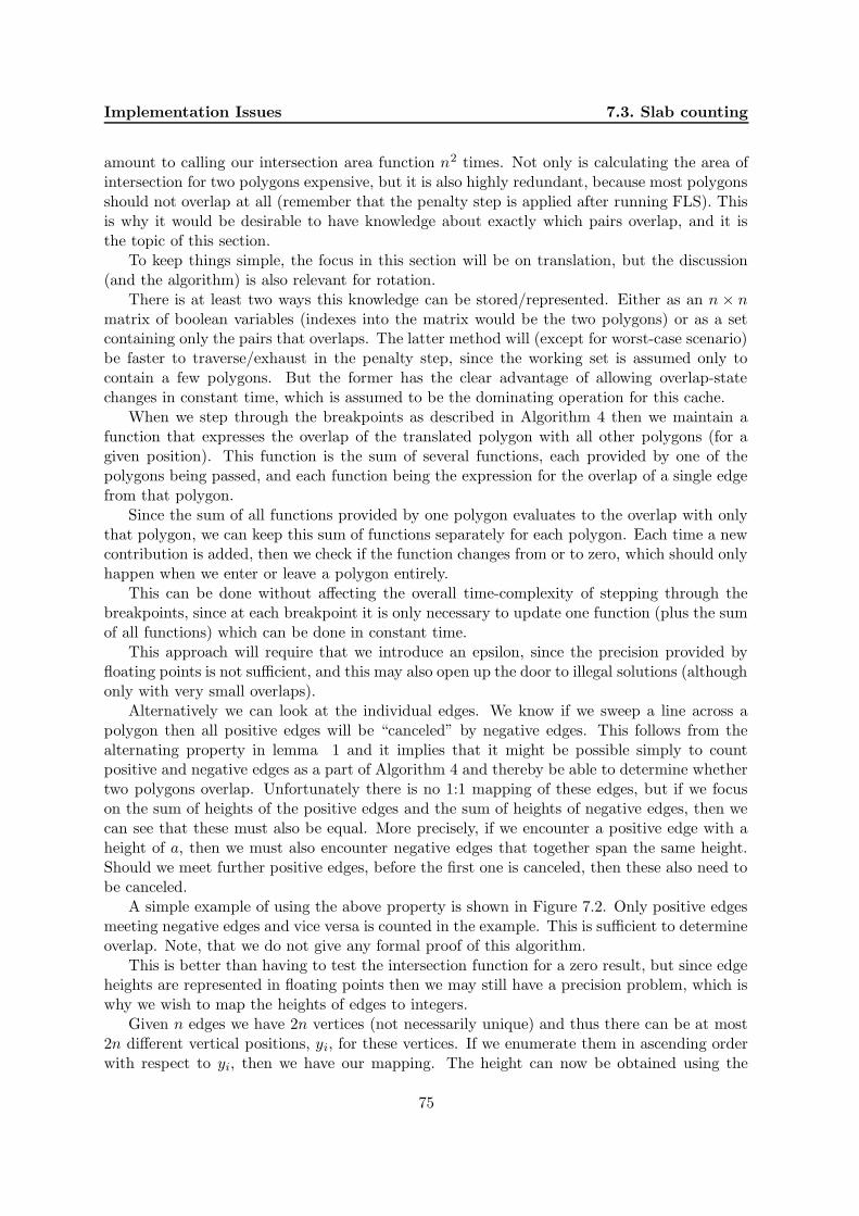
Implementation Issues 7.3. Slab counting
amount to calling our intersection area function n2 times. Not only is calculating the area ofintersection for two polygons expensive, but it is also highly redundant, because most polygonsshould not overlap at all (remember that the penalty step is applied after running FLS). Thisis why it would be desirable to have knowledge about exactly which pairs overlap, and it isthe topic of this section.
To keep things simple, the focus in this section will be on translation, but the discussion(and the algorithm) is also relevant for rotation.
There is at least two ways this knowledge can be stored/represented. Either as an n × nmatrix of boolean variables (indexes into the matrix would be the two polygons) or as a setcontaining only the pairs that overlaps. The latter method will (except for worst-case scenario)be faster to traverse/exhaust in the penalty step, since the working set is assumed only tocontain a few polygons. But the former has the clear advantage of allowing overlap-statechanges in constant time, which is assumed to be the dominating operation for this cache.
When we step through the breakpoints as described in Algorithm 4 then we maintain afunction that expresses the overlap of the translated polygon with all other polygons (for agiven position). This function is the sum of several functions, each provided by one of thepolygons being passed, and each function being the expression for the overlap of a single edgefrom that polygon.
Since the sum of all functions provided by one polygon evaluates to the overlap with onlythat polygon, we can keep this sum of functions separately for each polygon. Each time a newcontribution is added, then we check if the function changes from or to zero, which should onlyhappen when we enter or leave a polygon entirely.
This can be done without affecting the overall time-complexity of stepping through thebreakpoints, since at each breakpoint it is only necessary to update one function (plus the sumof all functions) which can be done in constant time.
This approach will require that we introduce an epsilon, since the precision provided byfloating points is not sufficient, and this may also open up the door to illegal solutions (althoughonly with very small overlaps).
Alternatively we can look at the individual edges. We know if we sweep a line across apolygon then all positive edges will be “canceled” by negative edges. This follows from thealternating property in lemma 1 and it implies that it might be possible simply to countpositive and negative edges as a part of Algorithm 4 and thereby be able to determine whethertwo polygons overlap. Unfortunately there is no 1:1 mapping of these edges, but if we focuson the sum of heights of the positive edges and the sum of heights of negative edges, then wecan see that these must also be equal. More precisely, if we encounter a positive edge with aheight of a, then we must also encounter negative edges that together span the same height.Should we meet further positive edges, before the first one is canceled, then these also need tobe canceled.
A simple example of using the above property is shown in Figure 7.2. Only positive edgesmeeting negative edges and vice versa is counted in the example. This is sufficient to determineoverlap. Note, that we do not give any formal proof of this algorithm.
This is better than having to test the intersection function for a zero result, but since edgeheights are represented in floating points then we may still have a precision problem, which iswhy we wish to map the heights of edges to integers.
Given n edges we have 2n vertices (not necessarily unique) and thus there can be at most2n different vertical positions, yi, for these vertices. If we enumerate them in ascending orderwith respect to yi, then we have our mapping. The height can now be obtained using the
75

7.3. Slab counting Implementation Issues
a
b
c d
e
f
g
a b
c d
a
b
c d
e
f
g h+
1
a
b
cd
e
f
g h+
1
h−2
a
b
cd
e
f
g h+
1
h−2
h−3
h−4
Figure 7.2: A simple example of using the height of slabs to determine overlap. a) Two polygonsare given. Positive edges are bolded. b) The first breakpoint is when the negative edge a startscrossing the positive edge g. The height of their overlap is h+
1 c) The second relevant breakpointis when the positive edge c stops crossing edge d. The height of their overlap is h−2 . d) Thelast relevant breakpoints is when the positive edges b and c stops crossing edge e. The heightsof their overlaps are h−3 and h−4 . It is easy to see that h+
1 − (h−2 + h−3 + h−4 ) = 0, which meansthat there is no longer any overlap.
76

Implementation Issues 7.4. Incorporating penalties in translation
mapped coordinates, and these heights will always be integers.Since we split the plane into slabs (of different heights) then we refer to the height of an
edge, in the mapped slab-coordinates, as slab count, since it is in fact just the number of slabsthat the edge spans.
Algorithm 5 shows how to calculate the slab counts with respect to horizontal translation.Calculating the slab counts for vertical translation is only a matter of using horizontal positionsinstead of vertical positions.
Algorithm 5 Slab counting
Input: An array of breakpoints, Breakpoints, each having MinY,MaxY valuescorresponding to the vertical extent of overlap of the involved lines.Initialize a sorted set, Y Positions. Initially empty.for i = 1 to Breakpoints.size do
Y Positions.add(Breakpoints[i].MinY ).Y Positions.add(Breakpoints[i].MaxY ).
end forInitialize an empty mapping set, Y ToSlab.for i = 1 to Y Positions.size do
Y ToSlab[Y Positions[i]] = i.end forfor i = 1 to Breakpoints.size do
minY = Breakpoints[i].MinY .maxY = Breakpoints[i].MaxY .Breakpoints[i].SlabCount = Y ToSlab[maxY ]− Y ToSlab[minY ].
end for
The algorithm has 3 loops running O(k) iterations each (k being the number of break-points). If we assume that the mapping Y ToSlab uses perfect hashing then access to membersis constant and thus the two latter loops run in O(k) time. The first loop needs to updatea sorted set which would normally be O(log k) for each update (e.g. using red-black or AVLtrees) — this makes the entire loop run in O(k log k) and thus it is the dominating factor ofthis algorithm.
Since the breakpoints have already gone through a sorting-process then this extra step donot worsen the overall time complexity. Also note that there will be a lot of duplicate positionsso the expected running time of the above is probably closer to linear.
7.4 Incorporating penalties in translation
According to the description of how we have modified our objective function (see 3.2) then ourtranslation algorithm needs to be modified to take penalties into consideration when reportingthe optimal placement of a stencil. This is almost trivial since there is at least one breakpointeach time the overlap between two stencils change. Furthermore, there is at most one changein the slab-count at each breakpoint, so when changing the slab-count for a polygon, we checkto see if it changes from zero to non-zero or the opposite, and if so, add/subtract the penaltyto a variable expressing the accumulated penalties, which is then added to the price.
A non-trivial part of this scheme appears when we have several breakpoints (from differentpolygons) with the same offset. A possible situation is illustrated in Figure 7.3. Here we
77
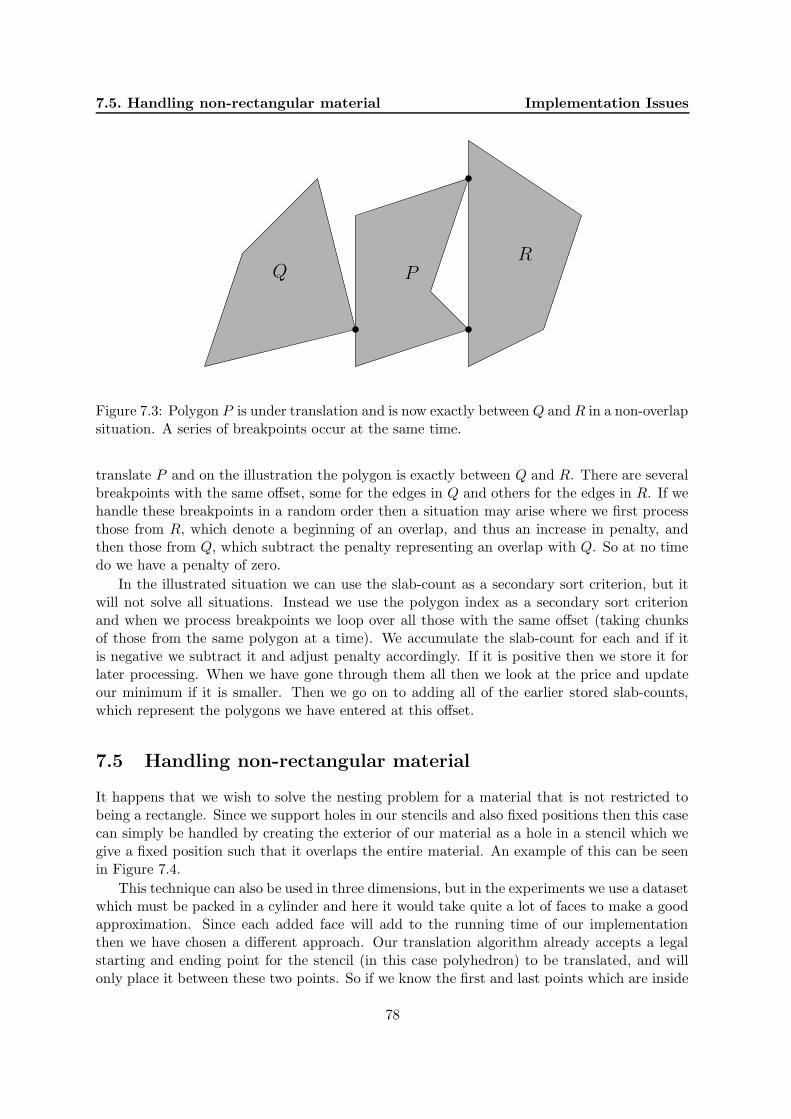
7.5. Handling non-rectangular material Implementation Issues
Q PR
Figure 7.3: Polygon P is under translation and is now exactly between Q and R in a non-overlapsituation. A series of breakpoints occur at the same time.
translate P and on the illustration the polygon is exactly between Q and R. There are severalbreakpoints with the same offset, some for the edges in Q and others for the edges in R. If wehandle these breakpoints in a random order then a situation may arise where we first processthose from R, which denote a beginning of an overlap, and thus an increase in penalty, andthen those from Q, which subtract the penalty representing an overlap with Q. So at no timedo we have a penalty of zero.
In the illustrated situation we can use the slab-count as a secondary sort criterion, but itwill not solve all situations. Instead we use the polygon index as a secondary sort criterionand when we process breakpoints we loop over all those with the same offset (taking chunksof those from the same polygon at a time). We accumulate the slab-count for each and if itis negative we subtract it and adjust penalty accordingly. If it is positive then we store it forlater processing. When we have gone through them all then we look at the price and updateour minimum if it is smaller. Then we go on to adding all of the earlier stored slab-counts,which represent the polygons we have entered at this offset.
7.5 Handling non-rectangular material
It happens that we wish to solve the nesting problem for a material that is not restricted tobeing a rectangle. Since we support holes in our stencils and also fixed positions then this casecan simply be handled by creating the exterior of our material as a hole in a stencil which wegive a fixed position such that it overlaps the entire material. An example of this can be seenin Figure 7.4.
This technique can also be used in three dimensions, but in the experiments we use a datasetwhich must be packed in a cylinder and here it would take quite a lot of faces to make a goodapproximation. Since each added face will add to the running time of our implementationthen we have chosen a different approach. Our translation algorithm already accepts a legalstarting and ending point for the stencil (in this case polyhedron) to be translated, and willonly place it between these two points. So if we know the first and last points which are inside
78

Implementation Issues 7.5. Handling non-rectangular material
Figure 7.4: An example of nesting inside an irregular material. It should be noted that thisis not a difficult nesting problem — it was found within 10 seconds using the implementednesting solver.
79

7.6. Approximating stencils Implementation Issues
Figure 7.5: Keeping polyhedra within the boundaries of a cylinder can as a rough approxima-tion be reduced to the problem of keeping a bounding box inside a circle.
the material, then we can make use of the above feature.
Assume that the height of the cylinder is along the z-axis. If we imagine we are translatingon the x-axis then given the y position of our polyhedron we can find the first and last xposition within the material by solving x2 = r2 − y2 for each point in the polyhedron. Inour implementation we have chosen an even simpler solution. The bounding box of polygonsprovides us with a rough approximation which will do for the data instances that we need topack — an illustration of the approach can be seen in Figure 7.5.
7.6 Approximating stencils
The speed of algorithms working with polygons almost always depend on the number of ver-tices. It has been suggested [37] to make both exterior and interior approximations of polygonsto help speed up any work done with the polygons. An exterior approximation is a polygonwhich contains the original polygon. This is very useful for the polygons to be packed sinceany legal placement with the approximated polygons will also be a legal placement with theoriginal polygons. Interior approximations are useful for simplifying the polygon(s) describingthe material. In the following we will focus on exterior approximations which in most casesare the most important since the material is very often rectangular. Note that if the materialis interpreted as an infinite polygon with one or more holes then we can also use the exteriorapproximation algorithm for the material.
If the area of the original polygon is A and the area of the exterior approximation is Ae
then we can measure the waste of an approximation as Ae−AAe
. Now we can state the problemof finding a good exterior approximation of an arbitrary shape, not necessarily a polygon, intwo different ways:
Problem 1: Using a fixed number of vertices, find an exterior approximation which wastesas little material as possible.
Problem 2: Given a maximum percentage of waste, find an exterior approximation usingas few vertices as possible.
80
Implementation Issues 7.6. Approximating stencils
The nesting problem is about maximizing the use of material and therefore it is importantto limit the amount of wasted material in the exterior approximations. In this regard, thesecond problem is a bit more adaptive than the first problem since some shapes will need morevertices in their approximations than others to keep the same level of waste. One could alsoimagine a combination of the two problems e.g. using a maximum waste per vertex.
It should be noted though that an optimal solution to the second problem is not necessarilythe best possible approximation to use in the nesting problem. It does not guarantee that theshape of the exterior approximation is close to the original polygon. Thin “spikes” could beintroduced in an approximation which would not waste much space, but they would make thenesting problem much harder.
Nevertheless we will focus on the second problem, but we will not find an optimal solution.We do not know the complexity of any of the stated problems, but we will present a heuristicsolution method which satisfies our needs for exterior approximations. The heuristic onlyworks for polygons.
The heuristic is greedy and it is based on a heuristic described by Heistermann andLengauer [37]. First we need to define the concept of border triangles. These come in twotypes and two very simple examples are given in Figure 7.6a and 7.6b. The vertices of apolygon can be divided into two different groups depending on the angle they make with theirneighboring vertices. An angle below 180 degrees indicates a concave vertex and an angleabove 180◦ indicates a convex vertex.
Using these we can find two different types of border triangles. Concave border trianglesare found by simply taking all concave vertices and use their neighboring vertices to maketriangles. Convex border triangles are a bit more subtle. These require two neighboring convexvertices and the third point of the triangle is found by extending the edges as shown in 7.6b(it is not possible if the combined left turn of the points exceed 180◦).
Now we can describe a very simple heuristic for approximating a polygon within a fixed per-centage of waste. Note that Heistermann and Lengauer [37] only use concave border trianglesin their approximation heuristic.
1. Find the border triangle of the current polygon with the smallest area.
2. If the waste of the polygon including this area is larger than the allowed amount of wastethen stop the process.
3. Otherwise, change the polygon to include the found area. For concave border trianglesthis is done by removing a vertex from the polygon. For convex border triangles thismeans to remove two vertices and adding a new one. In both cases the resulting polygonhas one vertex less.
4. Remove any self intersections caused by changing the polygon.
5. Now go back to step 1.
With the exception of the removal of self intersections the above algorithm is quite simple.As noted earlier though we have to look out for any spikes i.e. thin convex border triangleswith a small area. An extreme example is given in Figure 7.6c. We need to have anothercriterion for choosing the “smallest” border triangle. In Figure 7.6d there is a less extremeexample of convex border triangle. It is tempting to simply require that the angle α shouldbe greater than some fixed value, but this does not really reflect what we want. It is a bit
81

7.7. Center of a polygon Implementation Issues
a
b d
α
β γ
c
Figure 7.6: a) Three points making a right turn (counter clockwise) represent a concavity whichcan be removed by removing the middle point. b) Four points making two left turns (counterclockwise) which do not exceed 180◦ represent a convexity which can removed by adding anew point at the intersection of lines from the first and the last edge (and removing the twoobsolete points). c) An example of a convexity with a triangle of little area but significanttopological influence. It should be avoided to include such triangles in an approximation. d)A less extreme example of a triangle related to a convexity. It is not easy to determine whichtriangles to include.
too restrictive. A better alternative is to require that α is greater than at least one of the twoother angles β or γ.
Now, let us take a look at the algorithm in action. In Figure 7.7 a highly irregular polygonis reduced to a simple quadrilateral. It is also shown that the result is not optimal regardingminimum waste using 4 vertices. Also note that if only concave border triangles had beenremoved then the resulting polygon would have had 6 vertices.
Now by varying the maximum percentage of wasted material the heuristic can provide uswith different levels of approximated polygons. These can be used in other algorithms to speedup calculations when the original polygons are not strictly necessary.
In the above algorithm the waste is computed in relation to the polygon itself. This meansthat a border triangle of the same size on a small and on a large polygon will be evaluateddifferently. By considering all polygons at once when making the approximation this can beavoided and a better approximation might be found i.e. fewer vertices within the same bound.This is examined as a part of our experiments (Section 8.1.4).
7.7 Center of a polygon
For each polygon we need to determine a center of rotation. Intuitively, a really good choicewould be the center of the smallest enclosing circle (SEC) of all the vertices of the polygon.This will ensure that the focus is on improving the solution by rotating the polygon and notby translating it (we have the translation part of the neighborhood for that purpose).
Finding the SEC (also known as the minimal enclosing circle or minimum spanning circle)can (a bit surprising) be done in linear time [46]. Formally the problem is: Given a set ofpoints on the plane, find the smallest circle which encloses all of them.
82

Implementation Issues 7.7. Center of a polygon
a b
c d
e f
Figure 7.7: a) A highly irregular polygon with 11 vertices. b) The set of all border triangleswhich it is possible to remove. 2 convex and 5 concave border triangles. c-e) The triangleof smallest area is iteratively removed. The list of border triangles is updated at each step.f) Continuing as long as possible results in a polygon with just 4 vertices and naturally noconcavities. The dashed line indicates a quadrilateral with smaller area not found by thealgorithm.
83

7.7. Center of a polygon Implementation Issues
The O(n) algorithm is quite complicated, but luckily, we can find the SECs in a preprocess-ing step i.e. we do not need the algorithm to be linear in time. We can choose to implementa simple algorithm by Skyum [53] running in time O(n log n) or an even simpler algorithm byWelzl [57, 16] that runs in expected linear time. We have chosen the latter algorithm.
Note that when choosing the center of the enclosing circle as the center of rotation thenthe enclosing circle can also be used as a bounding circle. It will then be very simple to skipall polygons too far away to ever overlap the polygon to be rotated.
84

Chapter 8
Computational Experiments
8.1 2D experiments
8.1.1 Strategy
The following experiments should be viewed as complimentary to those which Egeblad etal. [28] conducted for their implementation, Jab. Although no source is shared between theimplementations the solution methods are very similar and so some choices have been basedon the experience gained from earlier experiments.
After a presentation of the data instances in the following section we will discuss andexperiment with the lambda value, approximation schemes and strip length strategy. Anexample with quality requirements is also given and finally some benchmark comparisons aredone with published results and with a commercial solver.
8.1.2 Data instances
The amount of publically available data instances is limited. Table 8.1 presents some statisticsabout the instances which we will use for our experiments and benchmarks. They vary between43 and 99 stencils per set and the average number of vertices per stencil is between 6 and 9with the exception of Swim which has 20 vertices per stencil. All of the sets can be seen inFigure 8.1 where it is also indicated that they all contain subsets of identical stencils. Notethat we do not utilize this property in any way and therefore it does not make the problemseasier for us.
Name Stencils Vertices (avg.) Area (avg.) Area (total) Strip width
Artificial 99 7.19 9.6 947 27Shapes0 43 9.09 37.1 1596 40Shapes2 28 6.29 11.7 328 15Shirts 99 6.05 22.1 2183 40Swim 48 20.00 530078.4 25443764 5600Trousers 64 6.06 269.0 17216 79
Table 8.1: Testdata
85
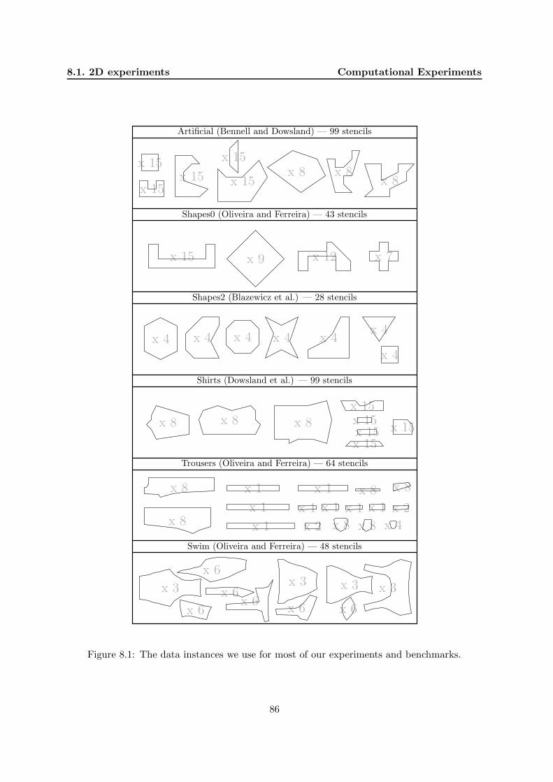
8.1. 2D experiments Computational Experiments
x 15x 15
x 15x 15
x 15x 8 x 8
x 8
Artificial (Bennell and Dowsland) — 99 stencils
x 15 x 9 x 12 x 7
Shapes0 (Oliveira and Ferreira) — 43 stencils
x 4 x 4 x 4 x 4 x 4x 4
x 4
Shapes2 (Blazewicz et al.) — 28 stencils
x 8 x 8 x 8 x 15
x 15x 15x 15x 15
Shirts (Dowsland et al.) — 99 stencils
x 8
x 8 x 1
x 1
x 1 x 1 x 8 x 8
x 1 x 1 x 1 x 1 x 2
x 2 x 8 x 8 x 4
Trousers (Oliveira and Ferreira) — 64 stencils
x 3
x 6
x 6
x 6x 6
x 3x 3
x 6 x 6
x 3
Swim (Oliveira and Ferreira) — 48 stencils
Figure 8.1: The data instances we use for most of our experiments and benchmarks.
86

Computational Experiments 8.1. 2D experiments
65 %
70 %
75 %
80 %
85 %
90 %
0.5 1 1.5 2 2.5 3 3.5 4 4.5
Utiliza
tion
Lambda
ArtificialShapes0Shapes2
ShirtsSwim
Trousers
Figure 8.2: Solution quality for different values of lambda after 5 minutes.
8.1.3 Lambda
Experiments regarding the value of lambda and FLS strategy were conducted by Egeblad etal. We are only going to repeat the lambda experiment to make sure that this value is setappropriately. We know from their experiments that this value should be in the range of1%-4% of the area of the largest stencil and we have tried values in this interval for all datainstances. The results can be seen in Figure 8.2 and they are quite inconclusive. We settle fora value of 3%.
8.1.4 Approximations
From our previous work with GLS we have already experienced that Swim is a time-consumingdataset to pack, and for this reason we have implemented an approximation strategy to reducethe number of vertices in the stencils which in this case must be polygons. The first experimentwe have done shows the number of vertices left in the dataset as a function of the maximumallowed waste and can be seen in Figure 8.3. To get an idea of how the dataset is affectedwe also present an example of exactly how Swim gets affected by an approximation allowing awaste of 5%, this can be seen in Figure 8.4.
To see if approximated vertices actually make a difference in the time used to find goodsolutions we have tried to solve Swim both with and without approximated vertices for anallowed waste of 2.5%, 4.0% and 5.0%. We have done this for all combinations of parameterstaken by our approximation scheme, see Section 7.6 for details, and the results can be seen inTable 8.2.
The conclusion must be that approximation is an advantage for the Swim dataset. Exactlyhow much waste one should allow, and which approximation scheme should be used, are stillopen questions. Since a waste percentage of 2.5 has the best average in solution quality wehave chosen to use this value, and furthermore to only use the concave approximation schemeand look at all stencils since that worked best for this percentage.
87

8.1. 2D experiments Computational Experiments
40
60
80
100
120
140
160
180
200
220
0 % 5 % 10 % 15 % 20 % 25 %
Num
ber
ofve
rtic
es
Waste
ConcaveConcave ConvexConcave Global
Concave Convex Global
Figure 8.3: The number of vertices left in the Swim instance when different levels of waste areallowed.
Waste 0.0% 2.5% 4.0% 5.0%
Concave 66.7% 67.4% 66.6% 64.1%Concave Convex 66.7% 67.7% 63.0% 64.2%Concave Global 66.7% 67.9% 65.4% 67.1%Concave Convex Global 66.7% 67.9% 65.4% 63.0%
Table 8.2: The utilization after one hour for different approximation parameters and wastethresholds.
Another way we have tried to speed up our implementation is by reducing each translationto a subset of the material (relative to the position of each stencil). This is given as a percentageof the materials size. Since we have already established that Swim benefits from approximatedvertices we will try this bounded translation both with and without approximated stencils, tosee if a) bounded translation can compete with approximated vertices and b) to see if boundedtranslation can further improve approximated vertices. Our findings can be seen in Figure 8.5and our conclusion is that, at least for Swim, bounded translation is not an advantage. Wehave skipped this idea for our further experiments.
8.1.5 Strip length strategy
As described earlier we can solve the strip-length problem as a decision problem where wedecrement the size of our material after each successful placement. The size of our decrementingstep is subject for the following experiment. The first thing we notice is that our datasets varysignificantly in size and thus a decrement step given in units make little sense. Instead we defineit as a percentage of the initial length — we have chosen 1% because smaller improvements areprobably of little interest (at least in the beginning). We could set it higher, but given enoughtime, our implementation should be able to reach the same solutions as can be found using ahigher initial stepping factor.
At some point we may have shrinked the length so much that 1% of the initial length is too
88

Computational Experiments 8.1. 2D experiments
Original stencils (219 vertices).
Each stencil reduced with concave triangles (129 vertices).
Each stencil reduced with concave and convex triangles (92 vertices).
Global approach looking at triangles in all stencils simultaneously (86 vertices).
Figure 8.4: The Swim data instance with various approximation schemes applied which allkeep the total waste below 5%.
89
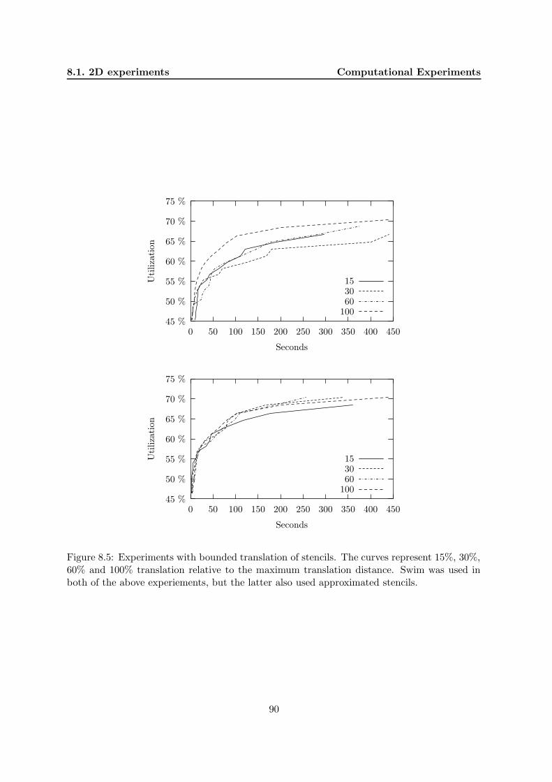
8.1. 2D experiments Computational Experiments
45 %
50 %
55 %
60 %
65 %
70 %
75 %
0 50 100 150 200 250 300 350 400 450
Utiliza
tion
Seconds
153060
100
45 %
50 %
55 %
60 %
65 %
70 %
75 %
0 50 100 150 200 250 300 350 400 450
Utiliza
tion
Seconds
153060
100
Figure 8.5: Experiments with bounded translation of stencils. The curves represent 15%, 30%,60% and 100% translation relative to the maximum translation distance. Swim was used inboth of the above experiements, but the latter also used approximated stencils.
90

Computational Experiments 8.1. 2D experiments
much of a step to find the next legal placement — for this reason we should introduce a wayto adapt our decremented size when such situations arise (and a way to find these situations).Though if we continue to make our decrementing step smaller then we may eventually end upwith an infinitely small step.
All this has resulted in the following 3 experiments.
• Always decrement by 1%, which we refer to as “fixed”.
• Decrement by 1% until 4n2 iterations have been executed without finding a legal place-ment. Make the decrement step 70% smaller and backtrack to last legal solution, whichwe refer to as “adaptive”.
• Same as above but using a lower limit of 0.1% of the length as a minimum for thedecrement step, referred to as “adaptive w/ LB”.
The results can be seen in Table 8.3 where each strategy has been tried for all instances andthe utilization obtained after one hours run is reported. A fourth strategy is also presentedwhich is not directly related to the stepping strategy. Here we test a simple rounding strategywhere we try to reduce the number of decimals, and thus the possible positions of stencils, byrounding the result from our translation to integer coordinates. It is presented in this tablesimply to make comparisons easier.
It is clear from this experiment that the adaptive approach with a lower bound is thebest choice for stepping strategy. Interestingly the rounding-strategy seemed to pay off on theartificial datasets (with rotation), but did not improve anything for the examples from thetextile industry (on the contrary), the reason for this is most likely that the artificial datasetshave been defined by humans and so have integer sizes.
Strategy Fixed Adaptive Adaptive w/ LB Rounded
No rotation
Artificial 69.9% 59.3% 70.8% 70.6%Shapes0 65.0% 64.9% 66.2% 66.4%Shapes2 78.9% 77.5% 80.8% 80.2%Shirts 84.6% 84.3% 84.3% 84.3%Swim 69.4% 69.7% 70.8% 70.2%Trousers 85.4% 85.8% 85.6% 85.7%
180◦ rotation
Artificial 73.8% 73.8% 74.4% 74.5%Shapes0 72.3% 71.4% 72.5% 72.5%Shapes2 80.1% 78.4% 81.1% 81.6%Shirts 85.6% 86.4% 86.5% 86.2%Swim 71.5% 72.9% 73.5% 72.9%Trousers 88.8% 89.5% 89.8% 89.2%
Table 8.3: The utilization for 3 different stepping-strategies and an attempt of a rounding-strategy.
91

8.1. 2D experiments Computational Experiments
Figure 8.6: The large boxes require quality Q2, the triangles require quality Q1 and the restrequire quality Q0. The striped pattern is of quality Q2 and the squared pattern is of qualityQ1. This legal placement was found within a few seconds by 2DNest.
8.1.6 Quality requirements
2DNest supports quality levels and requirements. As an example of this ability we createda simple (but ugly) animal hide data instance (guess an animal) with a few fixed areas withquality levels and a lot of small stencils with various quality requirements. This is illustratedin Figure 8.6.
8.1.7 Comparisons with published results
The data instances we are using have also frequently been used in existing literature. Someof the best results are gathered in Table 8.4 where they can be compared with results from2DNest. The computation times vary a lot, from minutes to hours, so the results should beinterpreted with care. Furthermore, the very small number of instances makes it difficult tomake any certain conclusions.
Nevertheless, Table 8.4 shows that we are doing quite well when it comes to solution quality.We believe that 2DNest has not been optimized to its full potential and that improvementsin solution strategies are still possible. Images of our placements for all 6 data instances canbe found in Appendix A (with 180◦ rotation).
It should be stated that the results reported for Jab are produced much faster than for2DNest and it is our general impression that our old implementation was faster than 2DNest
92

Computational Experiments 8.1. 2D experiments
Name 2DNest Jab Topos Jostling 2-exchange Hybrid.
No rotation
Artificial 70.8% - - - - (78.38%)1
Shapes0 66.2% 65.4% 59.8% 63.3% 61.4% 62.81%Shapes2 80.8% 77.1% - - - 76.58%Shirts 84.3% 84.4% - - - 81.18%Swim 68.3% 65.8% - - -Trousers 85.6% 84.4% - - -
180◦ rotation
Artificial 74.4% - - - - -Shapes0 72.5% 72.5% 65.4% 63.3% 67.6% -Shapes2 81.1% 77.1% 74.7% - 79.1% -Shirts 86.5% 85.7% 81.3% 83.1% 85.5% -Swim 71.0% 67.2% - - - -Trousers 89.8% 88.5% 82.8% - 88.6% -
Table 8.4: 2DNest (1 hour) is here compared with Jab by Egeblad et al. [28] (10 minutes),Topos by Oliveira et al. [51], Jostling for position by Dowsland et al. [23], 2-exchange byGomes and Oliveira [34] and a hybridized tabu search with optimization techniques by Bennelland Dowsland [7]
— especially in the early steps. Although we have not pinpointed the exact problem then wepresent here some plausible explanations.
• The use of double precision arithmetic is on average slower, however, it also introducessituations where stencils are repeatedly moved only small fractions of units, each provid-ing a very small improvement, and each opening up for another potential improvementon another translation axis — we did in fact experience such situations, but have triedto remedy them by setting an upper limit on the amount of allowed movements with thesame stencil and as can be seen from Table 8.3 then we have also tried a limited roundingstrategy. A better solution would be desirable.
• By using the described slab-counting we require that the solution is analytical legal,where our previous implementation allowed a very small overlap per stencil. This resultsin extra time spent each time a new legal solution has to be found.
• Our previous implementation used a better strategy to find an initial solution savingtime in the initial stage.
• Our current implementation is created with flexibility and adaptability in mind, whichcover using third party libraries like STL for data structures which although priced forits efficiency cannot compete with rolling your own solution.
1We were surprised by the result for Artificial and tried to examine it a bit closer. Correspondence with theauthors did not clarify the issue, but their solution method might be especially suited for this instance. Notethat our result is close to the result of the commercial solver presented in section 8.1.8.
93

8.1. 2D experiments Computational Experiments
8.1.8 Comparisons with a commercial solver
We have also obtained access to a commercial solver, AutoNester-T, which has been under de-velopment for about a decade. The results of this solver is very impressive especially regardingspeed. The following is a citation from the homepage of AutoNester-T:
“AutoNester-T combines many of the latest optimization techniques in order toachieve the best results in a very short time. We use local search algorithms basedon new variants of Simulated Annealing, multiply iterated greedy strategies, pairedwith efficient heuristics, pattern-recognition techniques, and fast Minkowski sumcalculators. In the local search algorithms, we use fully dynamic statistical coolingschedules and dynamic parameter choice.
For the calculation of optimality proofs and efficiency guarantees on markerswe use a combination of branch-and-bound algorithms and linear programming.”
It must be emphasized that AutoNester-T is optimized for marker making and thereforethe results of the artificial data instances (Artificial, Shapes0 and Shapes2) are not as good asfor the others (Shirts, Swim, Trousers). The results of AutoNester-T at various time points andour results after an hour is given in Table 8.5. AutoNester-T was run on a 600 MHz processor.The 2DNest results were obtained on a 1.4GHz processor. Note that AutoNester-T quicklyfinds very good solutions, but it seems that it does often not find better solutions when givenmore time. We know from experience with 2DNest that it often continues to find bettersolutions when given more time.
Test instance 2DNest 0.2 min. 1 min. 10 min.
No rotation
Artificial 70.8% 69.3% 70.1% 70.7%Shapes0 66.2% 61.4% 62.7% 64.4%Shapes2 80.8% 77.6% 78.8% 80.2%Shirts 84.3% 82.2% 83.6% 84.4% (2.2 min.)Swim 68.3% 69.4% 70.6% 71.4%Trousers 85.6% 83.8% 84.3% 84.5%
180◦ rotation
Artificial 74.4% 74.1% 75.9% 76.7% (2.8 min.)Shapes0 72.5% 68.8% 71.3% 71.3% (0.5 min.)Shapes2 81.1% 79.6% 81.1% 81.8% (2.9 min.)Shirts 86.5% 85.5% 86.8% 87.4% (1.8 min.)Swim 71.0% 74.4% 75.6% 75.6% (0.8 min.)Trousers 89.8% 89.3% 89.8% 90.6%
Table 8.5: These are results from the commercial solver AutoNester-T (version 3.5 [build3087]). Note how fast the solutions are generated. The results reported for 2DNest are witha 1 hour time limit.
1http://www.gmd.de/SCAI/optimierung/products/autonester-t/index.html
94

Computational Experiments 8.2. 3D experiments
8.2 3D experiments
8.2.1 Data instances
The amount of publically available data instances for the two-dimensional nesting problem islimited and it does not get better by adding a dimension to the problem. It is quite easyto obtain 3D objects from other areas of research, but these will typically have more than10000 faces each and would therefore require to be approximated as a first step. We have notimplemented an approximation algorithm for 3D objects and therefore this is not an option.
In the literature only one set of simple data instances has been used. They were originallycreated by Ilkka Ikonen and later used by Dickinson and Knopf [18] to compare their solutionmethod with Ikonen et al. [39]. There are eight objects available in the set and they arepresented in Table 8.6. Some of them have holes, but they are generally quite simple. Theycan all be drawn in two dimensions and then just extended in the third dimension. They haveno relation to real-world data instances. See them in Figure 8.7.
Name # Faces Volume Bounding box
Block1 12 4.00 1.00 × 2.00 × 2.00Part2 24 2.88 1.43 × 1.70 × 2.50Part3 28 0.30 1.42 × 0.62 × 1.00Part4 52 2.22 1.63 × 2.00 × 2.00Part5 20 0.16 2.81 × 0.56 × 0.20Part6 20 0.24 0.45 × 0.51 × 2.50Stick2 12 0.18 2.00 × 0.30 × 0.30Thin 48 1.25 1.00 × 3.00 × 3.50
Table 8.6: The Ikonen data set.
In the existing literature the above data set has been used with a cylindrical volume (whichis often the case for rapid prototyping machines). We have chosen to follow this approach sinceit will make it easier to compare results. This introduces the problem of keeping the objectwithin the limits of a cylinder. We handle this in a simple way using the bounding box of theobjects. This means that a small part of the real solution space is not available (which is ahandicap), but this simplification has no or only a minor effect on each of the objects in theabove table.
8.2.2 Statistics
The number of intersection calculations needed to find a solution was used by Dickinson andKnopf [18] to compare their solution method with the one by Ikonen et al. [39]. Unfortunatelywe are not able to do the same since we do not make intersection calculations in the same way.Execution times can be compared and we will do so in a benchmark at the end of this chapter.
In the following we will try to gather some statistics about the average behavior of oursolution method. A simple knapsack scheme has been implemented to pack as much as possiblewithin a cylinder of height 5.5 and radius 3.5. Within 2 minutes 54 objects have been packed(the 8 Ikonen objects are simply repeatedly added one by one) and they fill 34% of the volumeof the cylinder. About 3500 translations were done per minute. The packing can be seen fromfour different angles in Figure 8.8.
95

8.2. 3D experiments Computational Experiments
Part2 Part3 Part4
Part5 Part6 stick2
block1 thin
Figure 8.7: The Ikonen data set.
96

Computational Experiments 8.2. 3D experiments
Figure 8.8: Various aspects of a solution produced by a simple knapsack scheme.
97

8.2. 3D experiments Computational Experiments
8.2.3 Benchmarks
We have already presented the only available set of data instances for which there exists com-parable results 8.2.1. Two test cases are created by Dickinson and Knopf for their experiments.
• Case 1Pack 10 objects into a cylinder of radius 3.4 and height 3.0. The 10 objects are chosenas follows: 3 times Part2, 1 Part4 and 2 times Part3, Part5 and Part6. Total number offaces is 260 and 11.3% of the total volume is filled.
• Case 2Pack 15 objects into a cylinder of radius 3.5 and height 5.5. The 15 objects are chosenas in case 1, but with 5 more Part2. Total number of faces is 380 and 12.6% of the totalvolume is filled
Dickinson and Knopf report execution times for both their own solution method (serialpacking) and the one by Ikonen et al. (genetic algorithm). They ran the benchmarks on a 200MHz AMD K6 processor. The results are presented in Table 8.7 in which results from ouralgorithm is included. Our benchmarks were run on a 733MHz G4.
A random initial placement might be a problem since it could quite likely contain almostno overlap. Then it would not say much about our algorithm — especially the GLS part. Tomake the two cases a bit harder we doubled the number of objects. The results can be seenin Table 8.7 where it is compared with the results of Ikonen et al. and Dickinson and Knopf.Even considering the difference in processor speeds there is no doubt that our method is thefastest. The placements can be seen in Figure 8.9.
Test Ikonen et al. Dickinson and Knopf 3DNest
Case 1 22.13 min. 45.55 sec. 3.2 sec. (162 translations)Case 2 26.00 min. 81.65 sec. 8.1 sec. (379 translations)
Table 8.7: Execution times for 3 different heuristic approaches. Note that the number ofobjects are doubled for 3DNest.
98

Computational Experiments 8.2. 3D experiments
Case 1 Case 2
Figure 8.9: The above illustrations contain twice as many objects as originally intended inIkonens Case 1 and 2. They took only few seconds to find.
99

8.2. 3D experiments Computational Experiments
100

Chapter 9
Conclusions
The nesting problem has been described in most of its variations. Various geometric approachesto the problem has been described and a survey has been given of the existing literatureconcerning the nesting problem in two and three dimensions.
The major theoretical contributions of this thesis in relation to previous work is the fol-lowing. A proof of correctness of the translation algorithm presented by Egeblad et al. [28], ageneralization of the algorithm which among other things provides an algorithm for rotationand an easy generalization to three-dimensional nesting.
Furthermore, a comprehensive implementation of a two-dimensional nesting solver hasbeen created and it can handle a wide range of problem variations with various constraints.It performs very well compared with other solution methods even though it has not beenoptimized to its full potential. A three-dimensional nesting solver has also been implementedproving in practice that a fast translation method is also possible in this case. The results arepromising although only limited comparisons have been possible.
Subjects for future work include three-dimensional rotation and additional experiments tooptimize the solution strategies for various problem types.
Acknowledgements
The authors would like to thank the following people. Jens Egeblad for his participation inthe project on which this thesis is based, Ralf Heckmann for allowing us to access SCAIscommercial nesting program, Julia Bennell for providing 2D data instances and for mailinghard-to-obtain articles, and finally, John Dickinson for providing the 3D data instances.
101

Conclusions
102

Bibliography
[1] M. Adamowicz and A. Albano. Nesting two-dimensional shapes in rectangular modules.Computer Aided Design, 1:27–33, 1976.
[2] A. Albano. A method to improve two-dimensional layout. Computer Aided Design,9(1):48–52, 1977.
[3] A. Albano and G. Sappupo. Optimal allocation of two-dimensional irregular shapes usingheuristic search methods. IEEE Transactions on Systems, Man and Cybernetics, 5:242–248, 1980.
[4] R. C. Art, Jr. An approach to the two dimensional, irregular cutting stock problem.Technical Report 36.Y08, IBM Cambridge Scientific Center, September 1966.
[5] T. Asano, A. Hernandez-Barrera, and S. C. Nandy. Translating a convex polyhedron overmonotone polyhedra. Computational Geometry, 23:257–269, 2002.
[6] J. A. Bennell and K. A. Dowsland. A tabu thresholding implementation for the irregularstock cutting problem. International Journal of Production Research, 37:4259–4275, 1999.
[7] J. A. Bennell and K. A. Dowsland. Hybridising tabu search with optimisation techniquesfor irregular stock cutting. Management Science, 47(8):1160–1172, 2001.
[8] J. Blazewicz, P. Hawryluk, and R. Walkowiak. Using a tabu search approach for solvingthe two-dimensional irregular cutting problem. Annals of Operations Research, 41:313–325, 1993.
[9] J. Blazewicz and R. Walkowiak. A local search approach for two-dimensional irregularcutting. OR Spektrum, 17:93–98, 1995.
[10] E. K. Burke and G. Kendall. Applying ant algorithms and the no fit polygon to the nestingproblem. In Proceedings of the 12th Australian Joint Conference on Artificial Intelligence(AI’99), volume 1747, pages 454–464. Springer Lecture Notes in Artificial Intelligence,1999.
[11] E. K. Burke and G. Kendall. Applying evolutionary algorithms and the no fit polygonto the nesting problem. In Proceedings of the 1999 International Conference on ArtificialIntelligence (IC-AI’99), volume 1, pages 51–57. CSREA Press, 1999.
[12] E. K. Burke and G. Kendall. Applying simulated annealing and the no fit polygon to thenesting problem. In Proceedings of the World Manufacturing Congres, pages 70–76. ICSCAcademic Press, 1999.
103

Bibliography
[13] J. Cagan, D. Degentesh, and S. Yin. A simulated annealing-based algorithm using hierar-chical models for general three-dimensional component layout. Computer Aided Design,30(10):781–790, 1998.
[14] J. Cohen, A. Varshney, D. Manocha, G. Turk, H. Weber, P. Agarwal, F. Brooks,and W. Wright. Simplification envelopes. Computer Graphics, 30(Annual ConferenceSeries):119–128, 1996.
[15] W. Cook and A. Rohe. Computing minimum-weight perfect matchings. INFORMS Jour-nal on Computing, 11:138–148, 1999.
[16] M. de Berg, M. van Kreveld, M. Overmars, and O. Schwarzkopf. Computational Geometry,Algorithms and Applications. Springer-Verlag, 1997.
[17] J. K. Dickinson and G. K. Knopf. Generating 3d packing arrangements for layered man-ufacturing. In International Conference on Agile, Intelligent, and Computer-IntegratedManufacturing, Troy, New York, 1998. Rensselaer Polytechnic Institute.
[18] J. K. Dickinson and G. K. Knopf. Serial packing of arbitrary 3d objects for optimizinglayered manufacturing. In Intelligent Robots and Computer Vision XVII, volume 3522,pages 130–138, 1998.
[19] J. K. Dickinson and G. K. Knopf. A moment based metric for 2-D and 3-D packing.European Journal of Operational Research, 122(1):133–144, 2000.
[20] J. K. Dickinson and G. K. Knopf. Packing subsets of 3d parts for layered manufacturing.International Journal of Smart Engineering System Design, 4(3):147–161, 2002.
[21] D. Dobkin, J. Hershberger, D. Kirkpatrick, and S. Suri. Computing the intersection-depthof polyhedra. Algorithmica, 9:518–533, 1993.
[22] K. A. Dowsland and W. B. Dowsland. Solution approaches to irregular nesting problems.European Journal of Operational Research, 84:506–521, 1995.
[23] K. A. Dowsland, W. B. Dowsland, and J. A. Bennell. Jostling for position: Local im-provement for irregular cutting patterns. Journal of the Operational Research Society,49:647–658, 1998.
[24] K. A. Dowsland, S. Vaid, and W. B. Dowsland. An algorithm for polygon placement usinga bottom-left strategy. European Journal of Operational Research, 141:371–381, 2002.
[25] H. Dyckhoff. A typology of cutting and packing problems. European Journal of Opera-tional Research, 44:145–159, 1990.
[26] H. Dyckhoff, G. Scheithauer, and J. Terno. Cutting and packing: An annotated bibliog-raphy. In M. Dell’Amico, F. Maffioli, and S. Martello, editors, Annotated Bibliographiesin Combinatorial Optimizations, pages 393–412. John Wiley & Sons, 1996.
[27] J. Edmonds and E. L. Johnson. Matching, Euler tours and the Chinese postman. Math-ematical Programming, 5:88–124, 1973.
[28] J. Egeblad, B. K. Nielsen, and A. Odgaard. Metaheuristikken Guided Local Search anvendtpa pakning af irregulære polygoner, 2001.
104
Bibliography
[29] H. A. Eiselt, M. Gendreau, and G. Laporte. Arc routing problems, part II: The RuralPostman Problem. Operations Research, 43:399–414, 1995.
[30] L. Euler. Solutio problematis ad geometriam situs pertinentis. Commentarii AcademiaePetropolitanae, 8:128–140, 1736.
[31] R. J. Fowler, M. S. Paterson, and S. L. Tanimoto. Optimal packing and covering in theplane are np-complete. Information Processing Letters, 12(3):133–137, 1981.
[32] O. Færø, D. Pisinger, and M. Zachariasen. Guided local search for the three-dimensionalbin packing problem. To appear in INFORMS Journal on Computing, (2002).
[33] M. Garey and D. Johnson. Computers and intractability. A Guide to the theory of NP-completeness. W. H. Freeman and Company, New York, 1979.
[34] A. M. Gomes and J. F. Oliveira. A 2-exchange heuristic for nesting problems. EuropeanJournal of Operational Research, 141:359–370, 2002.
[35] R. Heckmann and T. Lengauer. A simulated annealing approach to the nesting problemin the textile manufacturing industry. Annals of Operations Research, 57:103–133, 1995.
[36] R. Heckmann and T. Lengauer. Computing closely matching upper and lower bounds ontextile nesting problems. European Journal of Operational Research, 108:473–489, 1998.
[37] J. Heistermann and T. Lengauer. The nesting problem in the leather manufacturingindustry. Annals of Operations Research, 57:147–173, 1995.
[38] E. Hopper and B. C. H. Turton. A review of the application of meta-heuristic algorithmsto 2D strip packing problems. Artificial Intelligence Review, 16:257–300, 2001.
[39] I. Ikonen, W. E. Biles, A. Kumar, J. C. Wissel, and R. K. Ragade. A genetic algorithm forpacking three-dimensional non-convex objects having cavities and holes. In Proceedings ofthe 7th International Conference on Genetic Algortithms, pages 591–598, East Lansing,Michigan, 1997. Morgan Kaufmann Publishers.
[40] P. Jain, P. Fenyes, and R. Richter. Optimal blank nesting using simulated annealing.Journal of mechanical design, 114:160–165, 1992.
[41] S. Jakobs. On genetic algorithms for the packing of polygons. European Journal ofOperational Research, 88:165–181, 1996.
[42] J. K. Lenstra and A. H. G. Rinnooy Kan. On general routing problems. Networks,6:273–280, 1965.
[43] Z. Li and V. Milenkovic. Compaction and separation algorithms for non-convex polygonsand their applications. European Journal of Operational Research, 84:539–561, 1995.
[44] A. Lodi, S. Martello, and M. Monaci. Two-dimensional packing problems: A survey.European Journal of Operational Research, 141:241–252, 2002.
[45] H. Lutfiyya, B. McMillin, P. Poshyanonda, and C. Dagli. Composite stock cutting throughsimulated annealing. Journal of Mathematical and Computer Modelling, 16(2):57–74,1992.
105

Bibliography
[46] N. Megiddo. Linear-time algorithms for linear programming in R3 and related problems.
SIAM Journal on Computing, 12(4):759–776, 1983.
[47] V. J. Milenkovic. Rotational polygon containment and minimum enclosure using onlyrobust 2D constructions. Computational Geometry, 13:3–19, 1999.
[48] V. J. Milenkovic. Densest translational lattice packing of non-convex polygons. Compu-tational Geometry, 22:205–222, 2002.
[49] V. J. Milenkovic, K. M. Daniels, and Z. Li. Automatic marker making. In Proceedingsof the Third Canadian Conference on Computational Geometry, pages 243–246. Shermer,Ed., Simon Fraser University, Vancouver, B.C., 1991.
[50] J. F. Oliveira and J. S. Ferreira. Algorithms for nesting problems. Applied SimulatedAnnealing, pages 255–273, 1993.
[51] J. F. Oliveira, A. M. Gomes, and J. S. Ferreira. TOPOS - a new constructive algorithmfor nesting problems. OR Spektrum, 22:263–284, 2000.
[52] T. Osogami. Approaches to 3D free-form cutting and packing problems and their appli-cations: A survey. Technical Report RT0287, IBM Research, Tokyo Research Laboratory,1998.
[53] S. Skyum. A simple algorithm for computing the smallest enclosing circle. InformationProcessing Letters, 37(3):121–125, 1991.
[54] Y. Stoyan, M. Gil, T. Romanova, J. Terno, and G. Scheithauer. Construction of a Φ-function for two convex polytopes, 2000.
[55] V. E. Theodoracatos and J. L. Grimsley. The optimal packing of arbitrarily-shaped poly-gons using simulated annealing and polynomial-time cooling schedules. Computer methodsin applied mechanics and engineering, 125:53–70, 1995.
[56] Chris Voudouris and Edward Tsang. Guided local search and its application to the trav-eling salesman problem. European Journal of Operational Research, 113:469–499, 1999.
[57] E. Welzl. Smallest enclosing disks (balls and ellipsoids). In H. Maurer (Ed.), New Resultsand New Trends in Computer Science, LNCS 555, pages 359–370. Springer-Verlag, 1991.
[58] X. Yan and P. Gu. A review of rapid prototyping technologies and systems. ComputerAided Design, 28(4):307–318, 1996.
106

Appendix A
Placements
Artificial
Shapes0
107

Placements
Shapes2
Shirts
108

Placements
Swim
Trousers
109