MCMC Methods for Functions: Modifying Old Algorithms to Make ...

Fast MCMC Algorithms on Polytopes
Raaz Dwivedi, Department of EECS
Joint work with Yuansi Chen Martin Wainwright Bin Yu
Random Sampling
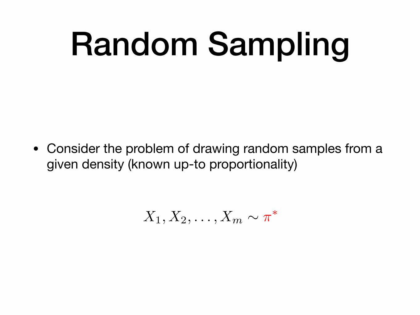
• Consider the problem of drawing random samples from a given density (known up-to proportionality)
X1, X2, . . . , Xm ⇠ ⇡⇤

Applications
• Probabilities of Events • Rare Event Simulations • Bayesian Posterior Mean • Volume Computation (polynomial time)
X1, X2, . . . , Xm ⇠ ⇡⇤
E[g(X)] =
Zg(x)⇡⇤(x)dx ⇡ 1
m
mX
i=1
g(Xi)

Applications
• Probabilities of Events • Rare Event Simulations • Bayesian Posterior Mean • Volume Computation (polynomial time)
X1, X2, . . . , Xm ⇠ ⇡⇤
E[g(X)] =
Zg(x)⇡⇤(x)dx ⇡ 1
m
mX
i=1
g(Xi)

Applications
• Zeroth order optimization: Polynomial time algorithms based on Random Walk
• Convex optimization: Bertsimas and Vempala 2004, Kalai and Vempala 2006, Kannan and Narayanan 2012, Hazan et al. 2015
• Non-convex optimization, Simulated Annealing: Aarts and Korst 1989, Rakhlin et al. 2015
minx2K
g(x)

Uniform Sampling on Polytopes
n linear constraints
d dimensions
n > d
X =
⇢x 2 Rd
���� Ax b
�
Uniform Sampling on Polytopes
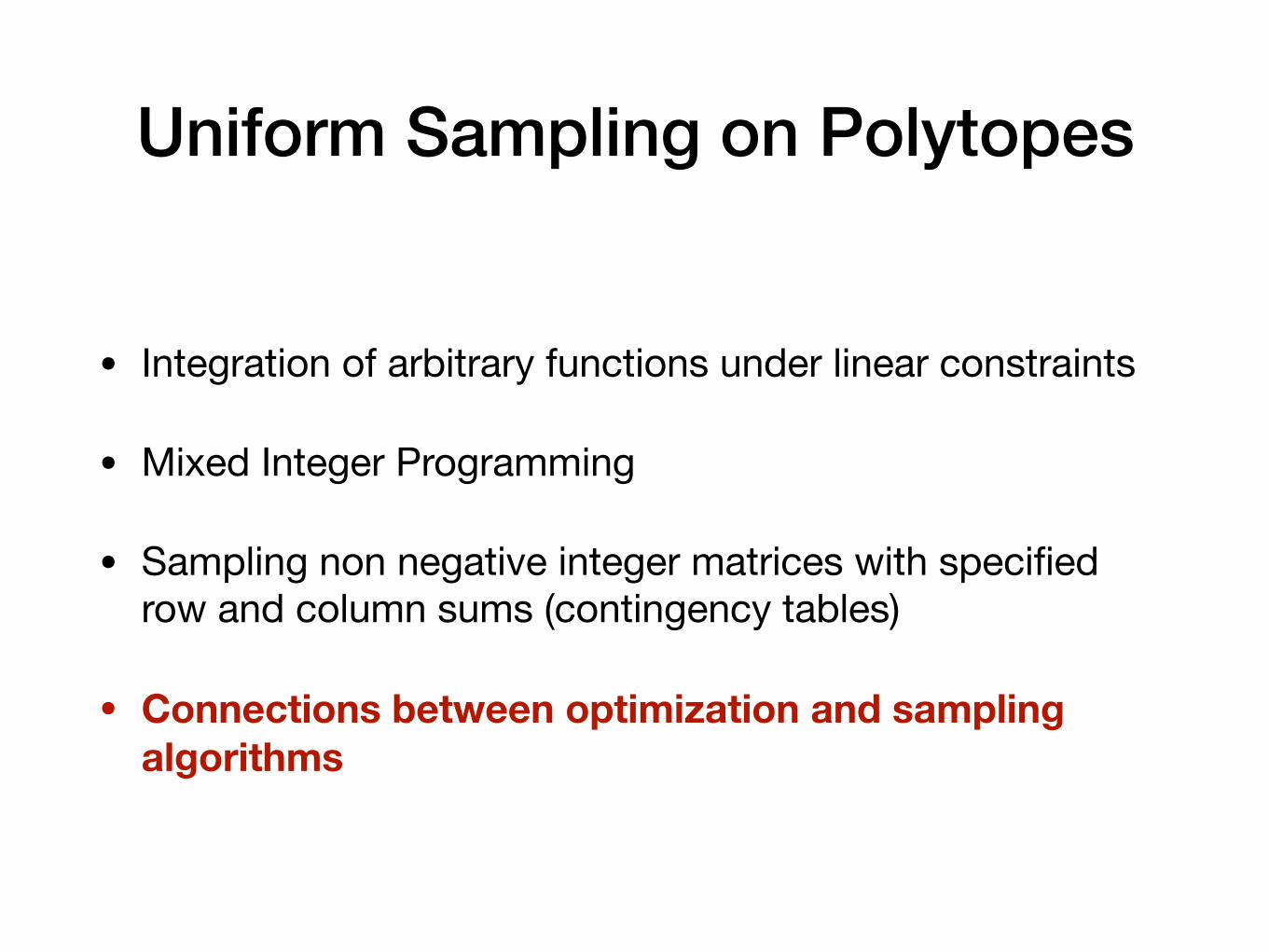
• Integration of arbitrary functions under linear constraints
• Mixed Integer Programming
• Sampling non negative integer matrices with specified row and column sums (contingency tables)
• Connections between optimization and sampling algorithms

GoalGiven A and b, and a starting distribution ,
design an MCMC algorithm
that generates a random sample from uniform distribution on
in as few steps as possible!
Convergence Rate: Mixing time for total variation
µ0
kµ0Pk � ⇡⇤kTV ✏
X =
⇢x 2 Rd
���� Ax b
�

Markov Chain Monte Carlo
• Design a Markov Chain which can converge to the desired distribution • Metropolis Hastings Algorithms (1950s), Gibbs Sampling (1980s)
• Simulate the Markov chain for several steps to get a sample

Markov Chain Monte Carlo
• Sampling on convex sets: Ball Walk (Lovász et al. 1990), Hit-and-run (Smith et al. 1993, Lovász 1999),
• Sampling on polytopes: Dikin Walk (Kannan and Hariharan 2012, Hariharan 2015, Sachdeva and Vishnoi 2016), Geodesic Walk (Lee and Vempala 2016)

Ball Walk [Lovász and Simonovits 1990]
• Propose a uniform point in a ball around x
• reject if outside the polytope, else move to it
z
z
z ⇠ UB✓x,
cpd
◆�

z
z
Ball Walk [Lovász and Simonovits 1990]
• Many rejections near sharp corners
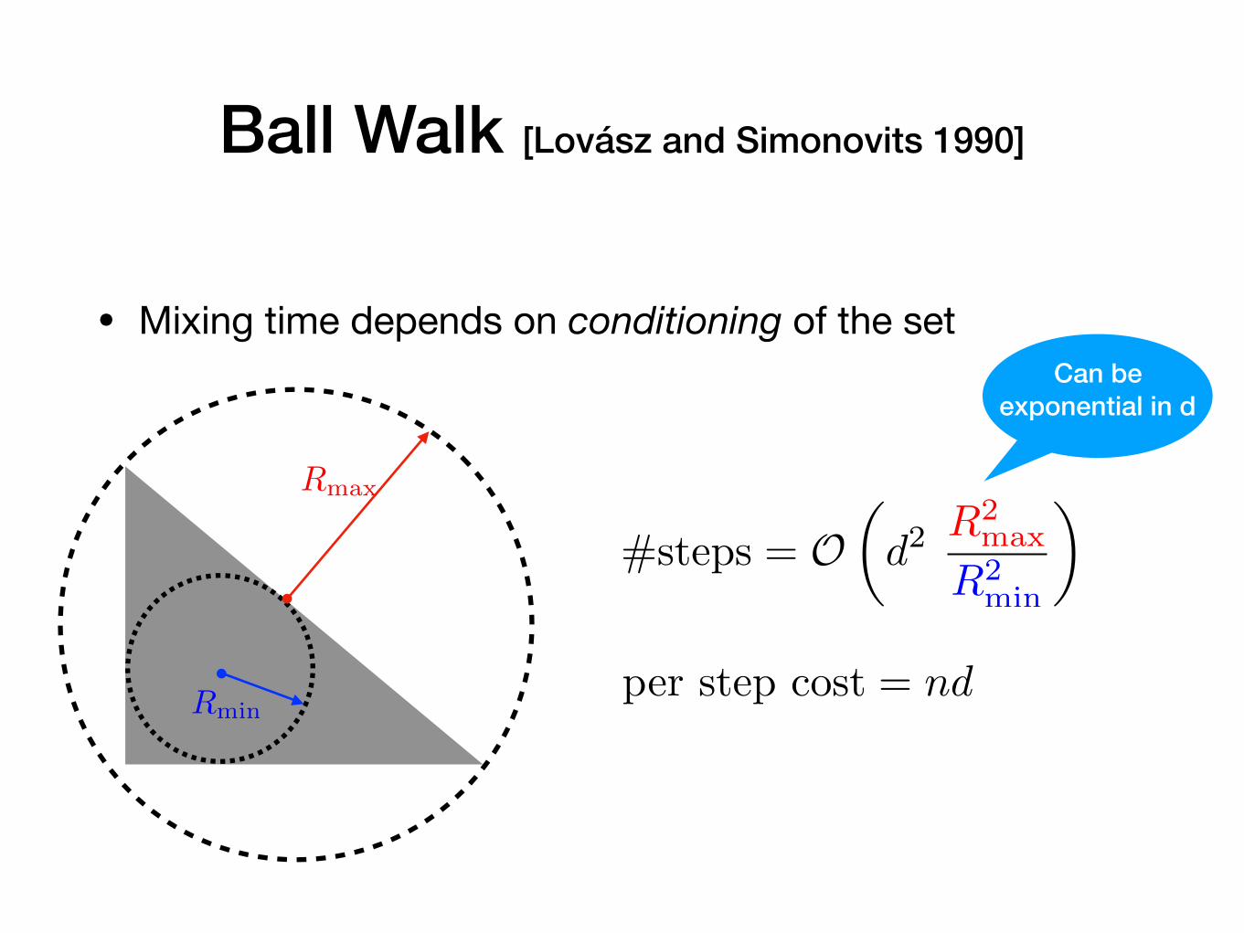
Ball Walk [Lovász and Simonovits 1990]
• Mixing time depends on conditioning of the set
Rmin
Rmax
#steps = O
✓d2
R2max
R2min
◆
per step cost = nd
Can be exponential in d

May be a variable shape ellipsoid?
z
z

• Proposal
• Another variant
• Accept Reject:
Dikin Walk [Kannan and Narayanan 2012]
z
z
z ⇠ N✓x,
r2
dD�1
x
◆
P( accept z) = min
⇢1,
P (z ! x)
P (x ! z)
�
z ⇠ U [Dx(r)]
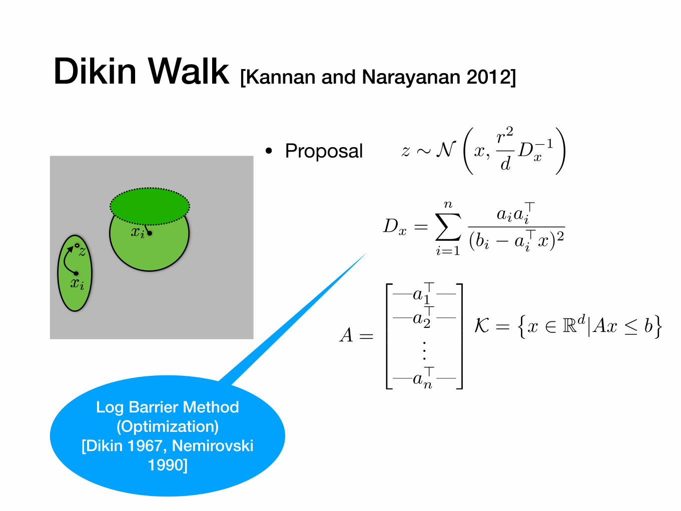
• Proposal
Dikin Walk [Kannan and Narayanan 2012]
z
zDx =
nX
i=1
aia>i(bi � a>i x)
2
A =
2
6664
—a>1 ——a>2 —
...—a>n—
3
7775K =
�x 2 Rd|Ax b
Log Barrier Method (Optimization)
[Dikin 1967, Nemirovski 1990]
z ⇠ N✓x,
r2
dD�1
x
◆
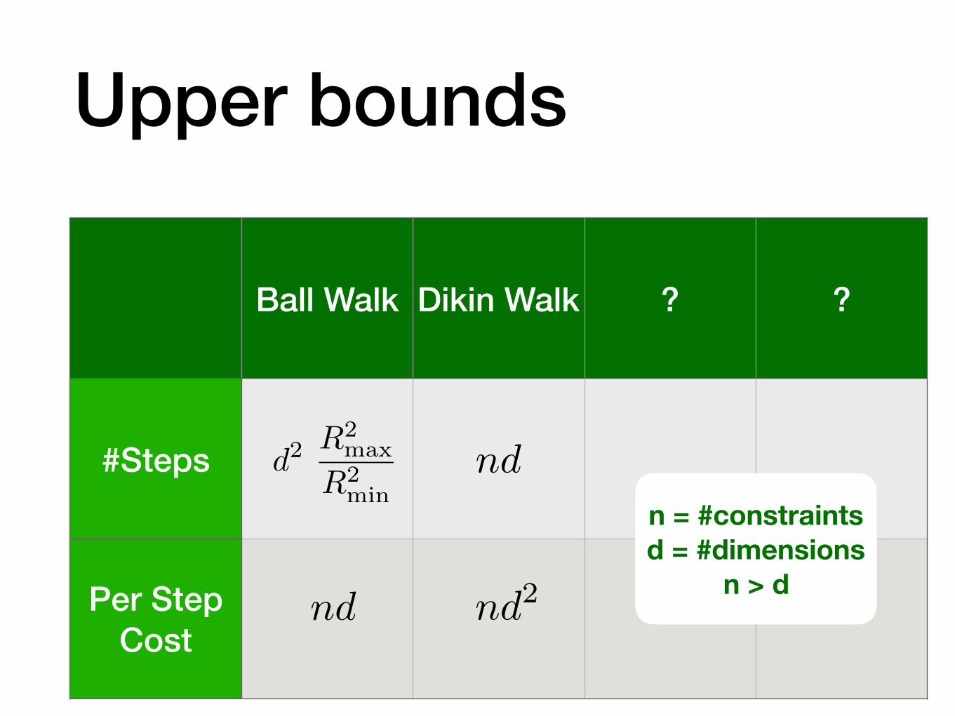
Upper bounds
Ball Walk Dikin Walk ? ?
#Steps
Per Step Cost
nd
nd
n = #constraints d = #dimensions
n > dnd2
d2R2
max
R2min
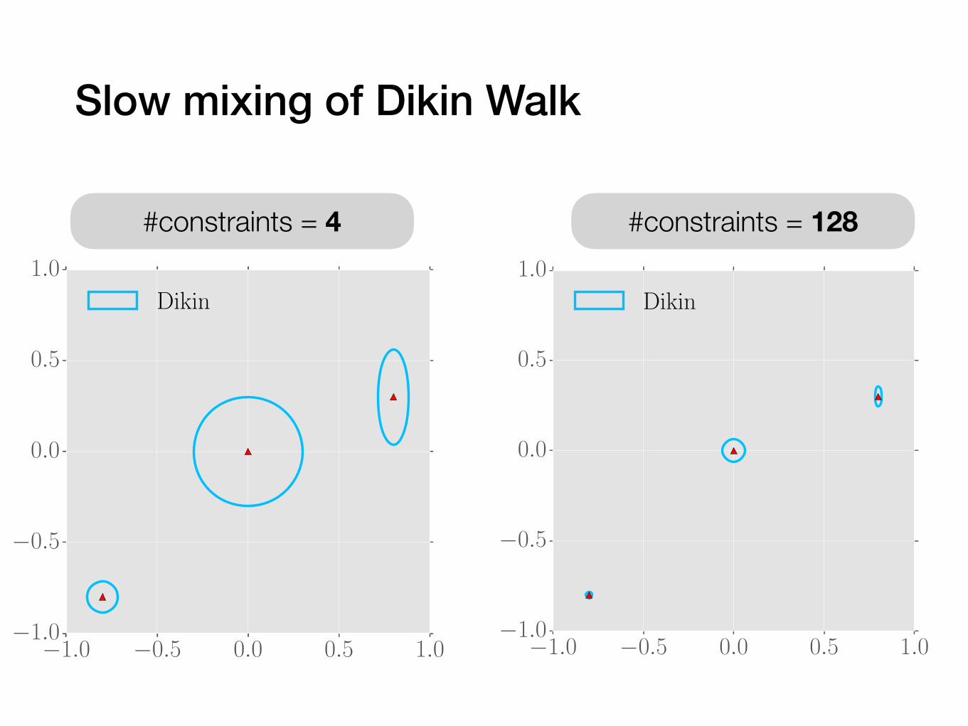
Slow mixing of Dikin Walk
�1.0 �0.5 0.0 0.5 1.0�1.0
�0.5
0.0
0.5
1.0
Dikin
�1.0 �0.5 0.0 0.5 1.0�1.0
�0.5
0.0
0.5
1.0
Dikin
#constraints = 128#constraints = 4

–Lovász’s Lemma
“If any two points that are apart have overlap in their transition regions, then the chain mixes in
steps.”
�
(Distance and overlap measured in appropriately)
⇢
O
✓1
�2⇢2
◆
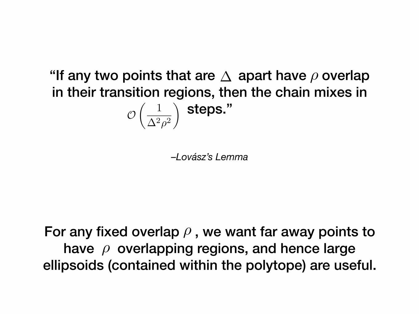
–Lovász’s Lemma
“If any two points that are apart have overlap in their transition regions, then the chain mixes in
steps.”
� ⇢
O
✓1
�2⇢2
◆
For any fixed overlap , we want far away points to have overlapping regions, and hence large
ellipsoids (contained within the polytope) are useful.
⇢⇢

Improving Dikin Walk
Dikin Proposal
z ⇠ N✓x,
r2
dD�1
x
◆
Dx =nX
i=1
aia>i(bi � a>i x)
2
nX
i=1
wi(x)aia>i
(bi � a>i x)2
Importance weighting of constraints

Log Barrier Method [Dikin 1967, Nemirovski 1990]
Dikin Proposal
z ⇠ N✓x,
r2
dD�1
x
◆
Dx =nX
i=1
aia>i(bi � a>i x)
2
[Kannan and Narayanan 2012]
Improving Dikin Walk

Sampling meets optimization (again!!)
Volumetric Barrier Method [Vaidya 1993]
[Chen, D., Wainwright and Yu 2017]
Log Barrier Method [Dikin 1967, Nemirovski 1990]
Dikin Proposal
z ⇠ N✓x,
r2
dD�1
x
◆
Dx =nX
i=1
aia>i(bi � a>i x)
2
[Kannan and Narayanan 2012]
Vaidya Proposal
z ⇠ N✓x,
r2pnd
V �1x
◆
Vx =nX
i=1
✓�x,i +
d
n
◆aia>i
(bi � a>i x)2
�x,i =a>i D
�1x ai
(bi � a>i x)2

Vaidya Walk [Chen, D., Wainwright, Yu 2017]
#constraints = 128#constraints = 4
�1.0 �0.5 0.0 0.5 1.0�1.0
�0.5
0.0
0.5
1.0
Dikin
Vaidya
�1.0 �0.5 0.0 0.5 1.0�1.0
�0.5
0.0
0.5
1.0
Dikin
Vaidya

Convergence Rates
Ball Walk Dikin Walk
Vaidya Walk
#Steps
Per Step Cost
n0.5d1.5nd
n constraints d dimensions
n > d
d2R2
max
R2min

Convergence Rates
Ball Walk Dikin Walk
Vaidya Walk
#Steps
Per Step Cost
n0.5d1.5nd
ndn constraints d dimensions
n > dnd2
d2R2
max
R2min
nd2

/ n0.45
�1.0 �0.5 0.0 0.5 1.0�1.0
�0.5
0.0
0.5
1.0
initial
�1.0 �0.5 0.0 0.5 1.0�1.0
�0.5
0.0
0.5
1.0
target
Dikin Walk vs Vaidya Walk
k = 0 k = 1
k = #iterations#experiments = 200#dimensions = 2

Dikin Walk
Vaidya Walk
k=10 k=100 k=500 k=1000
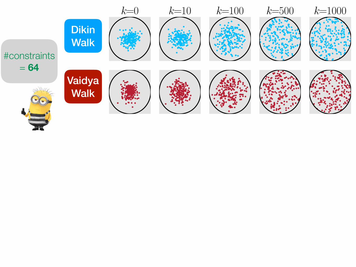
Dikin Walk vs Vaidya Walkk = #iterations#experiments = 200#constraints = 64

Dikin Walk
Vaidya Walk
k=10 k=100 k=500 k=1000
Dikin Walk vs Vaidya Walkk = #iterations#experiments = 200#constraints = 64

Dikin Walk
Vaidya Walk
k=10 k=100 k=500 k=1000
Dikin Walk vs Vaidya Walkk = #iterations#experiments = 200#constraints = 64

Dikin Walk
Vaidya Walk
k=10 k=100 k=500 k=1000
Small number of constraints: No Winner!
k = #iterations#experiments = 200#constraints = 64

Dikin Walk
Vaidya Walk
Dikin Walk vs Vaidya Walkk = #iterations#experiments = 200#constraints = 2048
k=10 k=100 k=500 k=1000

Dikin Walk
Vaidya Walk
Dikin Walk vs Vaidya Walkk = #iterations#experiments = 200#constraints = 2048
k=10 k=100 k=500 k=1000

Dikin Walk
Vaidya Walk
Dikin Walk vs Vaidya Walkk = #iterations#experiments = 200#constraints = 2048
k=10 k=100 k=500 k=1000

Dikin Walk
Vaidya Walk
Vaidya walk wins!k = #iterations#experiments = 200#constraints = 2048
k=10 k=100 k=500 k=1000
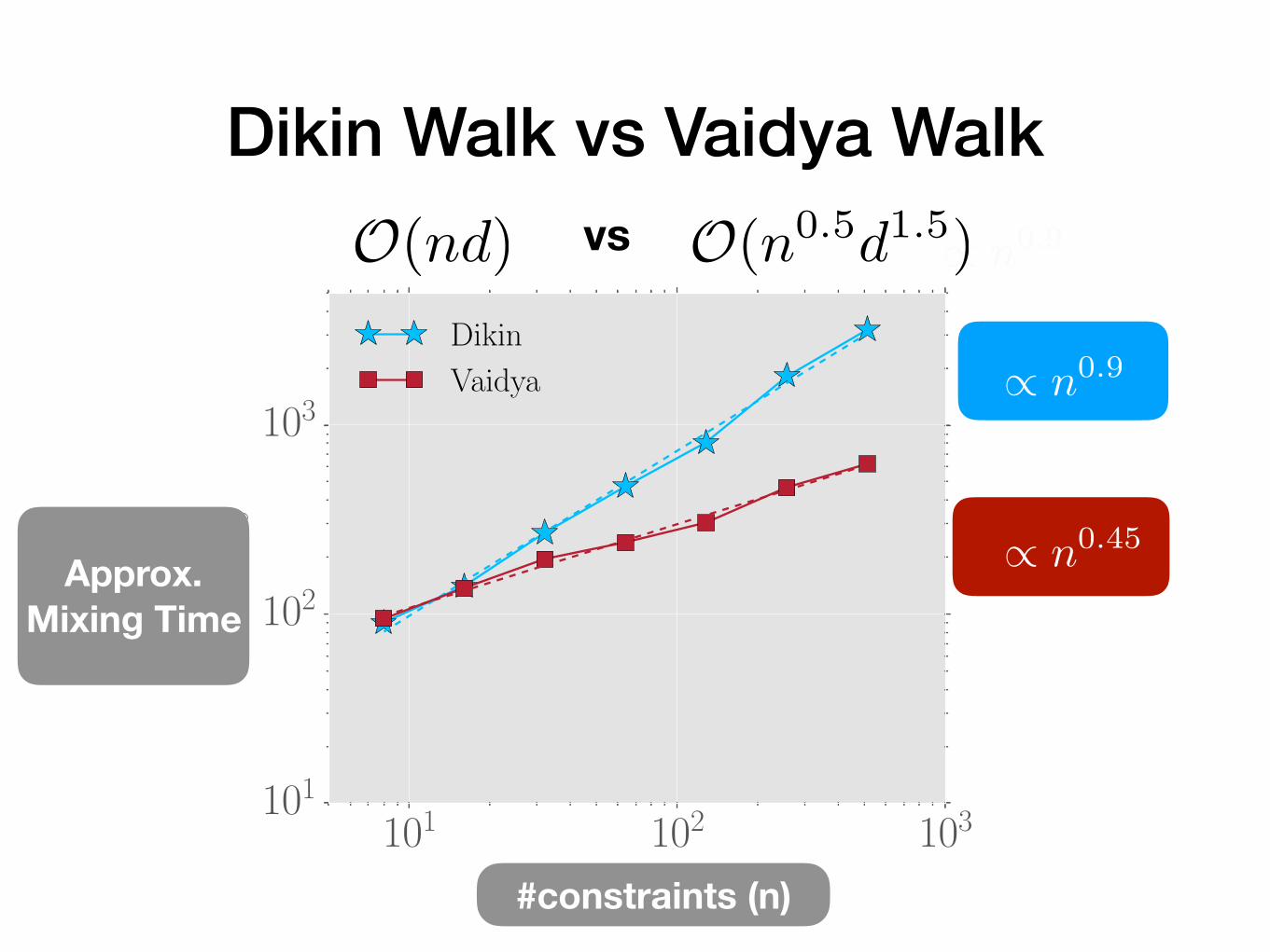
Dikin Walk vs Vaidya Walk/ n0.9
/ n0.45
O(nd) O(n0.5d1.5)
101 102 103
n
101
102
103
k̂ mix
Dikin
Vaidya / n0.9
/ n0.45
#constraints (n)
vs
Approx. Mixing Time
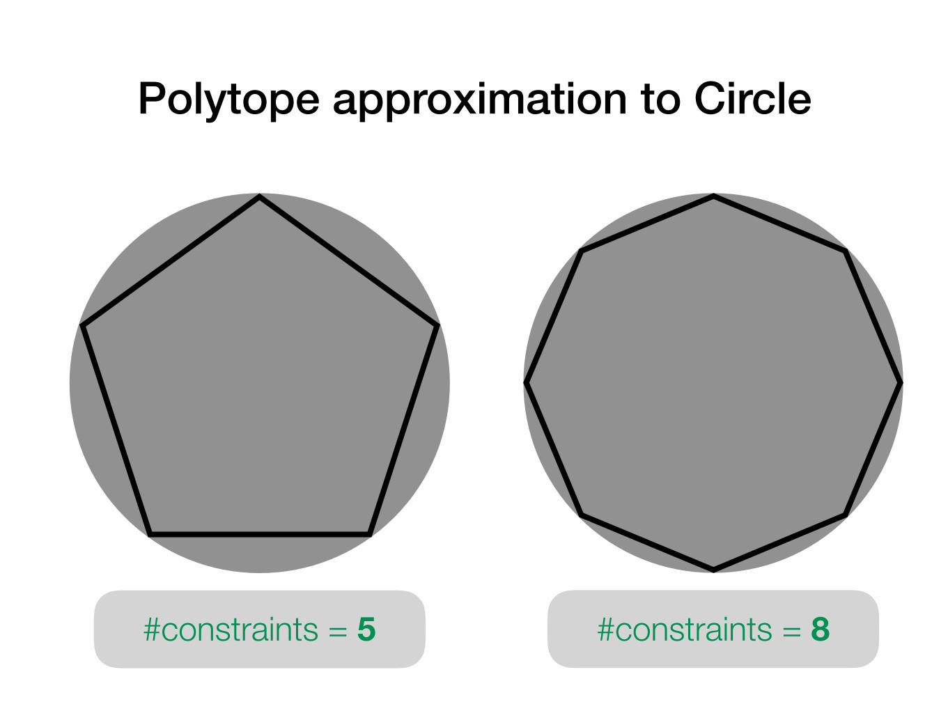
Polytope approximation to Circle
#constraints = 5 #constraints = 8
Dikin Walk
Vaidya Walk
k=0 k=10 k=100 k=500 k=1000
#constraints = 64

Dikin Walk
Vaidya Walk
k=0 k=10 k=100 k=500 k=1000
Dikin Walk
Vaidya Walk
#constraints = 64
#constraints = 2048
k=0 k=10 k=100 k=500 k=1000
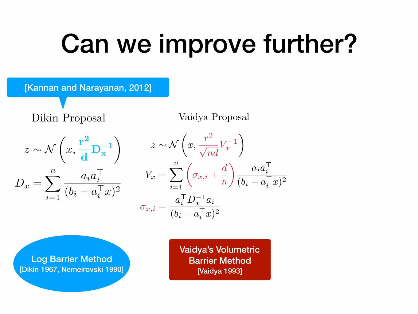
Can we improve further?
Log Barrier Method [Dikin 1967, Nemeirovski 1990]
Vaidya’s Volumetric Barrier Method
[Vaidya 1993]
Dikin Proposal
z ⇠ N✓x,
r2
dD�1
x
◆
Dx =nX
i=1
aia>i(bi � a>i x)
2
Vaidya Proposal
z ⇠ N✓x,
r2pnd
V �1x
◆
Vx =nX
i=1
✓�x,i +
d
n
◆aia>i
(bi � a>i x)2
�x,i =a>i D
�1x ai
(bi � a>i x)2
[Kannan and Narayanan, 2012]

John Walk
Log Barrier Method [Dikin 1967, Nemirovski 1990]
Vaidya’s Volumetric Barrier Method
[Vaidya 1993]
Dikin Proposal
z ⇠ N✓x,
r2
dD�1
x
◆
Dx =nX
i=1
aia>i(bi � a>i x)
2
Vaidya Proposal
z ⇠ N✓x,
r2pnd
V �1x
◆
Vx =nX
i=1
✓�x,i +
d
n
◆aia>i
(bi � a>i x)2
�x,i =a>i D
�1x ai
(bi � a>i x)2
John Proposal
z ⇠ N✓x,
r2
d1.5J�1x
◆
Jx =nX
i=1
jx,iaia>i
(bi � a>i x)2
jx,i = convex program
[Chen, D., Wainwright, Yu 2017][Kannan and Narayanan, 2012]
John’s Ellipsoidal Algorithm
[Fritz John 1948, Lee and Sidford 2015]
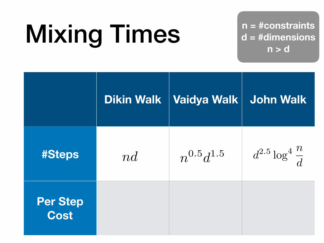
Mixing Times
Dikin Walk Vaidya Walk John Walk
#Steps
Per Step Cost
n0.5d1.5nd
n = #constraints d = #dimensions
n > d
d2.5 log4n
d

Mixing Times
Dikin Walk Vaidya Walk John Walk
#Steps
Per Step Cost
n0.5d1.5nd
n = #constraints d = #dimensions
n > d
d2.5 log4n
d
nd2 nd2 nd2 log2 n

Conjecture
Dikin Walk Vaidya Walk John Walk
#Steps
Per Step Cost
n0.5d1.5nd
n = #constraints d = #dimensions
n > d
nd2 nd2 nd2 log2 n
d2 logc⇣nd
⌘

– Numerical Experiments
“ For the John walk, the log factors are bottleneck in
practice. ’’

Proof Idea
• Proof relies on Lovasz’s Lemma
• Need to establish that near by points have similar transition distributions
• Have to show that the weighted matrices are sufficiently smooth — use of weights makes it involved

Summary
Optimization Sampling
Log Barrier Method1967, 1980s
Dikin Walk2012
Volumetric Barrier Method
1993
Vaidya Walk2017
John Ellipsoidal Algorithm
1948, 2015
John Walk2017
faster faster