Fast Interpolation and Time-Optimization on Implicit ...
8
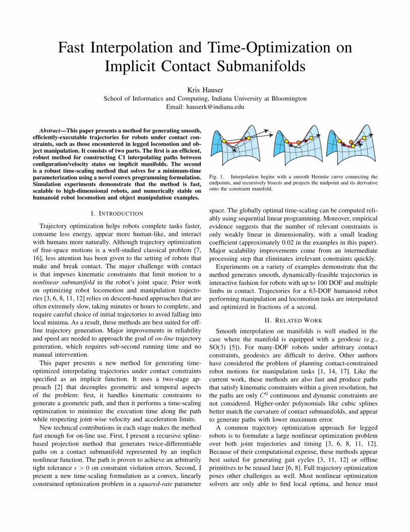
Fast Interpolation and Time-Optimization on Implicit Contact Submanifolds Kris Hauser School of Informatics and Computing, Indiana University at Bloomington Email: [email protected] Abstract—This paper presents a method for generating smooth, efficiently-executable trajectories for robots under contact con- straints, such as those encountered in legged locomotion and ob- ject manipulation. It consists of two parts. The first is an efficient, robust method for constructing C1 interpolating paths between configuration/velocity states on implicit manifolds. The second is a robust time-scaling method that solves for a minimum-time parameterization using a novel convex programming formulation. Simulation experiments demonstrate that the method is fast, scalable to high-dimensional robots, and numerically stable on humanoid robot locomotion and object manipulation examples. I. I NTRODUCTION Trajectory optimization helps robots complete tasks faster, consume less energy, appear more human-like, and interact with humans more naturally. Although trajectory optimization of free-space motions is a well-studied classical problem [7, 16], less attention has been given to the setting of robots that make and break contact. The major challenge with contact is that imposes kinematic constraints that limit motion to a nonlinear submanifold in the robot’s joint space. Prior work on optimizing robot locomotion and manipulation trajecto- ries [3, 6, 8, 11, 12] relies on descent-based approaches that are often extremely slow, taking minutes or hours to complete, and require careful choice of initial trajectories to avoid falling into local minima. As a result, these methods are best suited for off- line trajectory generation. Major improvements in reliability and speed are needed to approach the goal of on-line trajectory generation, which requires sub-second running time and no manual intervention. This paper presents a new method for generating time- optimized interpolating trajectories under contact constraints specified as an implicit function. It uses a two-stage ap- proach [2] that decouples geometric and temporal aspects of the problem: first, it handles kinematic constraints to generate a geometric path, and then it performs a time-scaling optimization to minimize the execution time along the path while respecting joint-wise velocity and acceleration limits. New technical contributions in each stage makes the method fast enough for on-line use. First, I present a recursive spline- based projection method that generates twice-differentiable paths on a contact submanifold represented by an implicit nonlinear function. The path is proven to achieve an arbitrarily tight tolerance > 0 on constraint violation errors. Second, I present a new time-scaling formulation as a convex, linearly constrained optimization problem in a squared-rate parameter Fig. 1. Interpolation begins with a smooth Hermite curve connecting the endpoints, and recursively bisects and projects the midpoint and its derivative onto the constraint manifold. space. The globally optimal time-scaling can be computed reli- ably using sequential linear programming. Moreover, empirical evidence suggests that the number of relevant constraints is only weakly linear in dimensionality, with a small leading coefficient (approximately 0.02 in the examples in this paper). Major scalability improvements come from an intermediate processing step that eliminates irrelevant constraints quickly. Experiments on a variety of examples demonstrate that the method generates smooth, dynamically-feasible trajectories in interactive fashion for robots with up to 100 DOF and multiple limbs in contact. Trajectories for a 63-DOF humanoid robot performing manipulation and locomotion tasks are interpolated and optimized in fractions of a second. II. RELATED WORK Smooth interpolation on manifolds is well studied in the case where the manifold is equipped with a geodesic (e.g., SO(3) [5]). For many-DOF robots under arbitrary contact constraints, geodesics are difficult to derive. Other authors have considered the problem of planning contact-constrained robot motions for manipulation tasks [1, 14, 17]. Like the current work, these methods are also fast and produce paths that satisfy kinematic constraints within a given resolution, but the paths are only C 0 continuous and dynamic constraints are not considered. Higher-order polynomials like cubic splines better match the curvature of contact submanifolds, and appear to generate paths with lower maximum error. A common trajectory optimization approach for legged robots is to formulate a large nonlinear optimization problem over both joint trajectories and timing [3, 6, 8, 11, 12]. Because of their computational expense, these methods appear best suited for generating gait cycles [3, 11, 12] or offline primitives to be reused later [6, 8]. Full trajectory optimization poses other challenges as well. Most nonlinear optimization solvers are only able to find local optima, and hence must
Transcript of Fast Interpolation and Time-Optimization on Implicit ...
Fast Interpolation and Time-Optimization onImplicit Contact Submanifolds
Kris HauserSchool of Informatics and Computing, Indiana University at Bloomington
Email: [email protected]
Abstract—This paper presents a method for generating smooth,efficiently-executable trajectories for robots under contact con-straints, such as those encountered in legged locomotion and ob-ject manipulation. It consists of two parts. The first is an efficient,robust method for constructing C1 interpolating paths betweenconfiguration/velocity states on implicit manifolds. The secondis a robust time-scaling method that solves for a minimum-timeparameterization using a novel convex programming formulation.Simulation experiments demonstrate that the method is fast,scalable to high-dimensional robots, and numerically stable onhumanoid robot locomotion and object manipulation examples.
I. INTRODUCTION
Trajectory optimization helps robots complete tasks faster,consume less energy, appear more human-like, and interactwith humans more naturally. Although trajectory optimizationof free-space motions is a well-studied classical problem [7,16], less attention has been given to the setting of robots thatmake and break contact. The major challenge with contactis that imposes kinematic constraints that limit motion to anonlinear submanifold in the robot’s joint space. Prior workon optimizing robot locomotion and manipulation trajecto-ries [3, 6, 8, 11, 12] relies on descent-based approaches that areoften extremely slow, taking minutes or hours to complete, andrequire careful choice of initial trajectories to avoid falling intolocal minima. As a result, these methods are best suited for off-line trajectory generation. Major improvements in reliabilityand speed are needed to approach the goal of on-line trajectorygeneration, which requires sub-second running time and nomanual intervention.
This paper presents a new method for generating time-optimized interpolating trajectories under contact constraintsspecified as an implicit function. It uses a two-stage ap-proach [2] that decouples geometric and temporal aspectsof the problem: first, it handles kinematic constraints togenerate a geometric path, and then it performs a time-scalingoptimization to minimize the execution time along the pathwhile respecting joint-wise velocity and acceleration limits.
New technical contributions in each stage makes the methodfast enough for on-line use. First, I present a recursive spline-based projection method that generates twice-differentiablepaths on a contact submanifold represented by an implicitnonlinear function. The path is proven to achieve an arbitrarilytight tolerance ε > 0 on constraint violation errors. Second, Ipresent a new time-scaling formulation as a convex, linearlyconstrained optimization problem in a squared-rate parameter
Fig. 1. Interpolation begins with a smooth Hermite curve connecting theendpoints, and recursively bisects and projects the midpoint and its derivativeonto the constraint manifold.
space. The globally optimal time-scaling can be computed reli-ably using sequential linear programming. Moreover, empiricalevidence suggests that the number of relevant constraints isonly weakly linear in dimensionality, with a small leadingcoefficient (approximately 0.02 in the examples in this paper).Major scalability improvements come from an intermediateprocessing step that eliminates irrelevant constraints quickly.
Experiments on a variety of examples demonstrate that themethod generates smooth, dynamically-feasible trajectories ininteractive fashion for robots with up to 100 DOF and multiplelimbs in contact. Trajectories for a 63-DOF humanoid robotperforming manipulation and locomotion tasks are interpolatedand optimized in fractions of a second.
II. RELATED WORK
Smooth interpolation on manifolds is well studied in thecase where the manifold is equipped with a geodesic (e.g.,SO(3) [5]). For many-DOF robots under arbitrary contactconstraints, geodesics are difficult to derive. Other authorshave considered the problem of planning contact-constrainedrobot motions for manipulation tasks [1, 14, 17]. Like thecurrent work, these methods are also fast and produce pathsthat satisfy kinematic constraints within a given resolution, butthe paths are only C0 continuous and dynamic constraints arenot considered. Higher-order polynomials like cubic splinesbetter match the curvature of contact submanifolds, and appearto generate paths with lower maximum error.
A common trajectory optimization approach for leggedrobots is to formulate a large nonlinear optimization problemover both joint trajectories and timing [3, 6, 8, 11, 12].Because of their computational expense, these methods appearbest suited for generating gait cycles [3, 11, 12] or offlineprimitives to be reused later [6, 8]. Full trajectory optimizationposes other challenges as well. Most nonlinear optimizationsolvers are only able to find local optima, and hence must

be provided with good initial trajectories. Another problem ismaintaining loop closure constraints at contacts. Some authorsparameterize the manifold of closed-loop configurations ateach possible contact state [3, 6, 8], while others enforce loopclosure implicitly by adding nonlinear equality constraints atcollocation points along the trajectory [11]. Parameterizationis manageable for a small number of contact states (e.g., leftfoot, right foot, and two foot support) but is challenging andtedious when hands, knees, and elbows may be involved incontact. Collocation is more versatile, but the accuracy ofclosure is proportional to the number of chosen grid points.Fine grids greatly increase computational cost and increase theprevalence of local minima in the optimization landscape.
Two-stage trajectory generation [2, 4] first computes a pathand then optimizes the speed according to dynamic constraintsin a second stage. This approach may fail to achieve thesame quality as full trajectory optimization because there isa risk of computing a path in stage 1 that will not yield afast time parameterization in stage 2, but results are usuallysatisfactory in practice given their orders of magnitude speedup. The classical method integrates the time scaling variablealong dynamic limits [2], but as identified in [9, 13], thismethod was found to suffer from numerical instability issues atdynamic singularities. Recent work formulated a more robustconvex optimization approach that casts time optimization as asecond-order cone program (SOCP) [15]. This paper presentsa simpler convex formulation that can be solved via sequentiallinear program (SLP), for which fast and robust implementa-tions are widely available. Scalability to very high-DOF robotsis improved by quickly pruning irrelevant constraints. As aresult the method solves 100D problems about as quickly asthe prior authors [15] solved a 6D one.
III. PROBLEM STATEMENT
Consider the problem of generating a trajectory y(t) :[0, T ] → Rn connecting start and goal configurations qs andqg and velocities qs and qg . It is required to satisfy kinematicconstraints C(q) = 0, with C : Rn → Rm a set of smooth,nonlinear constraints, and its first and second derivatives arerequired to satisfy velocity and acceleration bounds:
vL ≤y(t) ≤ vU for all t ∈ [0, T ] (1)aL ≤y(t) ≤ aU for all t ∈ [0, T ] (2)
where all inequalities are taken element-wise. It is assumedthat derivatives of C are nondegenerate when C(q) = 0 andthat there exists a Lipschitz constant M such that ‖C(p) −C(q)‖ ≤M‖p− q‖ for all p, q ∈ Rn.
The approach operates in two stages:1) Recursive Hermite projection. Constructs a continu-
ously differentiable geometric path p(s) : [0, 1] → Rnthat connects qs and qg and satisfies C(q) = 0.
2) Convex optimization time scaling. Optimizes a timeparameterization s(t) : [0, T ] → [0, 1] of p such thaty(t) = p(s(t)) satisfies (1–2) and minimizes T .
These two operations are roughly independent, and in particu-lar, the time-scaling method can be applied to arbitrary cubic
splines. Each will be described in more detail in the followingsections.
IV. RECURSIVE HERMITE PROJECTION
Recursive projection generates a continuously differentiable,piecewise polynomial path that satisfies C(q) = 0 within auser-specified tolerance ε. It begins with a interpolating cubicHermite curve in Rn and recursively bisects while projectingmidpoints onto C(q) = 0 (Fig. 1).
Hermite curves p(u) are cubic polynomials controlled byendpoints x0, x1 and tangent velocities v0, v1 such that thecurve satisfies p(0) = x0, p′(0) = v0, p(1) = x1, andp′(1) = v1. They can also be perfectly bisected into twoHermite curves pA(u) and pB(u) connected at the midpointp(0.5) with tangent p′(0.5).
Given a threshold ε on constraint violation errors and agrowth limit β ∈ (0.5, 1), recursive projection proceeds asfollows:
1) Begin with a Hermite curve p(u) connecting the startand end configurations. If no tangent directions areprescribed, obtain tangents by projecting the straight-line direction onto the nullspace of C(qs) and C(qg).
2) If len(p) ≤ 2ε/M , return ‘success’.3) Otherwise, subdivide p(u) into two Hermite curves
pA and pB , meeting at the midpoint (x, v) =(p(0.5), p′(0.5)).
4) Project x onto C(x) = 0 using a Newton-Raphsonsolver. Project v onto the nullspace of C(x). Let theresulting configuration and velocity be xm and vmrespectively.
5) Adjust pA and pB to meet at xm with derivatives vm.6) If max(len(pA), len(pB)) ≤ β · len(p), return ‘con-
vergence failure’. Otherwise, repeat Lines 2–5 on bothhalves.
See Fig. 1 for an illustration of these steps. The output is asequence of Hermite curves p1, . . . , pk as well as the fractionof the range [0, 1] maintained by each subsegment ∆1, . . . ,∆k
to map the original range into the subdivided sequence.The algorithm terminates when len(p) is small enough,
where len(p) is an upper bound on the length of the Hermitecurve (Fig. 2). To obtain this bound, it computes the length ofcorresponding Bezier polygon, len(p) = ‖P0 − P1‖+ ‖P1 −P2‖ + ‖P2 − P3‖. The growth condition in Line 5 ensurestermination in finite time, and that the projected path’s lengthis no more than a finite multiple of the length of the originalcurve p0 constructed in Line 1. Notice that at recursion depthd the condition len(p) ≤ βdlen(p0) must hold, so given thetolerance in Line 2, the terminal depth is no more than
dmax(ε, β) =log(2ε/M · len(p0))
log(β)+ 1 (3)
Hence the subdivided path may be no more than γ(ε, β) =(2β)dmax(ε,β) times as long as p0. All experiments use thevalue β = 0.9.
To interpolate multiple points, standard techniques can beused to generate a sequence of Hermite curves with smooth

P0
P1
P2
P3x0x1
v0 v1
ε/M {
P0
P1
P2
P3
(a) (b)
(c) (d)
Fig. 2. (a) Illustrating the recursion termination criterion, proving that thepath p lies within distance ε/M of the submanifold in configuration space,where M is a Lipschitz constant. (b) The Bezier polygon corresponding to p.(c) p is guaranteed to lie within the union of spheres centered at the endpoints,with radius equal to half the length of the Bezier polygon. The spheres failto satisfy the ε/M condition, so recursion continues. (d) After subdivision,both subsegments satisfy the condition and recursion stops.
tangent vectors at each point, e.g., Cardinal splines. Tangentsare projected to the manifold before recursive projectionbegins on each curve. The method can also be adapted to checkcollision and other infeasibility constraints during bisection,e.g., for use in motion planning. To do so, collisions arechecked at each midpoint xm in Line 4 and along all leafcurve segments at the end.
A. Properties of the Interpolator
If the algorithm is successful, the resulting spline:• Is C1 continuous.• At all curve endpoints, derivatives are tangent to the
constraint manifold.• Has arc-length no greater than γ(ε, β) · len(p0) where p0
is the initial curve.• Satisfies ‖C(p(u))‖ ≤ ε for all u ∈ [0, 1].
I now prove the latter claim.Theorem 1: The output path p(u) satisfies C(p(u)) ≤ ε for
all u ∈ [0, 1].Proof: The path is composed of small segments
p1, . . . , pk such that len(pi) ≤ 2ε/M for all i and C(pi(0)) =C(pi(1)) = 0. I shall prove that for any Hermite curve p,max0≤u≤1 ‖C(p(u))‖ ≤ M · len(p)/2, which implies thetheorem due to the termination condition in Step 2.
By the Lipschitz condition,
‖C(p(u))‖ = ‖C(p(u))− C(x0)‖ ≤M min ‖p(u)− x0‖, ‖p(u)− x1‖ (4)
and hence the problem is one of bounding the distance betweenpoints on p and the endpoints.
Hermite curves are equivalent to cubic Bezier curves withcontrol points P0 = x0, P1 = x0 + 1
3v0, P2 = x1 − 13v1, and
P3 = x1 (Fig. 2), and by the convex hull property, p(u) iscontained entirely within the convex hull of P0, . . . , P3. The
Fig. 3. Recursive projection can fail when recursion fails to make progressalong a manifold. This condition is detected in Line 5.
-1
-0.5
0
0.5
1
-1.5 -1 -0.5 0 0.5 1 1.5
-0.5
0
0.5
-1.5 -1 -0.5 0 0.5 1 1.5
Fig. 4. Interpolating on an implicit torus embedded in R3. Recursiveprojection successfully connects the source point (X) to almost all other pointson the torus, except for the indicated failure points (circles). Views from theside and above.
edges of this convex hull are some subset of P0P1, P0P2,P0P3, P1P2, P1P3, and P2P3. The next step in the proofensures that all of these edges are within the union of theballs B0 and B3 of radius len(p)/2 centered at each of p’sendpoints.
Obviously, P0P3 is contained within B0 ∪ B3 becauselen(p) ≥ ‖P3 − P0‖. Next, since a triangle with vertices A,B, C is completely contained within balls centered at A, Bwith radius 1
2 (‖A−B‖+ ‖B − C‖), the edges P0P1, P1P3,P0P2, and P2P3 are contained witihn B0∪B3. Finally, P1P2 iscontained within B0 ∪B3 because the midpoint of P1P2 canbe reached by walking along the Bezier polygon a distancelen(p)/2 from either endpoint.
Since the hull is contained within a distance of len(p)/2 ofeither endpoint of p, the entirety of p(u) is contained withinas well, and therefore ‖C(p(u))‖ ≤M · len(p)/2 as desired.
The interpolator is not complete; it may fail if 1) a midpointbecomes stuck in a local minima of ‖C(q)‖ during projection,and 2) the recursion fails to make progress along the manifold(Fig. 3). I evaluated how often the algorithm fails to connecttwo points on a torus, with target points taken on a regulargrid. Over 99% of the torus is successfully reached, and Fig. 4shows that failures occur only in a few narrow bands.
B. Interpolating on Submanifolds of Riemannian Manifolds
The interpolation algorithm can be extended to handle sub-manifolds of any geodesically complete Riemannian manifold

rather than Rn. These are needed to handle the base rotationsof mobile manipulators (SE(2)) and free-floating bases oflegged robots (SE(3)), for which straight lines do not properlyinterpolate along geodesics.
Let an arbitrary Riemannian manifoldM be equipped witha distance metric d(a, b) which provides the arc-length ofthe length minimizing path connecting points a and b, anda geodesic function g(t; a, b) which interpolates between aand b along such a length-minimizing path, with t ∈ [0, 1].The exponential map expq is defined such that g(t; a, b) =expa(tg(t; a, b)). The partial derivatives of g w.r.t. t, a, andb must also be supplied. Closed form expressions exist forSO(2) and SO(3) [10].
Hermite interpolation on M is performed using the classicde Casteljau construction of a Bezier curve [5]. Given endpoints x0, x1 ∈ M and tangents v0 ∈ Tx0M, v1 ∈ Tx1M,an interpolating curve is constructed first by calculating theBezier control points:
P0 = x0 P1 = expx0
(13v0
)P2 = expx1
(− 1
3v1
)P3 = x1
(5)
where P1 and P2 are extrapolated from the endpoints alongthe terminal tangent vectors. Then, the path p(u) is evaluatedvia the de Casteljau recurrences:
p(u) = g(u;P012(u), P123(u))
P012(u) = g(u;P01(u), P12(u))
P123(u) = g(u;P12(u), P23(u))
P01(u) = g(u;P0, P1)
P12(u) = g(u;P1, P2)
P23(u) = g(u;P2, P3)
(6)
With this expression, the recursive bisection algorithm pro-ceeds as usual except distances are replaced by d(·, ·) andp′(0.5) in Line 3 is computed via repeated application of thechain rule:
p′(u) =
(g +
∂g
∂aP ′012(u) +
∂g
∂bP ′123(u)
)∣∣∣∣u,P012(u),P123(u)
P ′012(u) =
(g +
∂g
∂aP ′01(u) +
∂g
∂bP ′12(u)
)∣∣∣∣u,P01(u),P12(u)
P ′01(u) = g(u;P0, P1)(7)
with similar formulas holding for P ′123, P ′12, and P ′23.
V. CONVEX OPTIMIZATION TIME SCALING
The time-scaling solves for a time parameterization s(t) ofthe path p that minimizes execution time T . The algorithm usea piecewise quadratic formulation of s(t), and demonstratethat with the proper parameterization this gives rise to aconvex program with linear inequalities. Dynamic feasibility isguaranteed over the entire time-scaled trajectory, rather thanjust at a finite set of points, due to the use of conservativeinterval bounding on the path’s derivatives.
s’s1 s2
s3
sN-2
s N-1. .
.
.
.
s0
t
ss1 s2 s3 sN-2 sN-1 sN...
T
s0 ss1 s2 s3 sN-2 sN-1 sN...
Fig. 5. A piecewise quadratic time-scaling s(t) is parameterized by the ratess0, . . . , sN .
The time scaling formulation rewrites y and y in terms ofp and s as follows:
y(t) = p′(s(t))s′(t) (8)
y(t) = p′′(s(t))s′(t)2 + p′(s(t))s′′(t). (9)
With p fixed, the problem of finding a dynamically-feasiblepath is reduced to one of finding a monotonically increasingmapping s(t) such that y and y given by (9) satisfy the con-ditions (1,2). The problem requires that s(t) to be continuousso that y is twice differentiable, and also that the trajectorystart and stop at zero velocity: s(0) = s(T ) = 0.
A. Parameterizing the time scaling by gridding the path do-main
Grid the path domain [0, 1] into N intervals [sk, sk+1],k = 0, . . . , N − 1 and let s(t) be piecewise quadratic on eachinterval. Let ∆sk be the duration of the k’th interval. Thisparameterization formulates s as a piecewise quadratic, twicedifferentiable curve parameterized by N + 1 rate parameterss0, . . . , sN at segment division points (Fig. 5).
Consider an interval k and its (unknown) time interval[tk, tk+1]. Over this interval, s(t) is fully determined by end-point velocities s′(tk) = sk and s′(tk+1) = sk+1. Verify thatthe following equation satisfies the desired terminal constraintson the interval [tk, tk+1] with ∆tk = tk+1 − tk = 2∆sk
sk+sk+1.
s(t) =s2k+1 − s2
k
4∆sk(t− tk)2 + sk(t− tk) + sk (10)
So, s′ is a linear interpolation between sk and sk+1 ands′′(t) = (s2
k+1 − s2k)/(2∆sk) is a constant independent of
u. Parameterizing in terms of u(t) = (s′(t)− sk)/(sk+1− sk)to map [tk, tk+1] to the range [0, 1], (9) becomes:
y(t(u)) =p′(s(u))((1− u)sk + usk+1) (11)
y(t(u)) =p′′(s(u))((1− u)sk + usk+1)2
+ p′(s(u))s2k+1 − s2
k
2∆sk(12)
These conditions must be satisfied for each interval k =1, . . . , N and u ∈ [0, 1].

B. Derivative bounding
The next step converts the continuous constraints (1,2)into finite ones. An interval arithmetic bounding technique isused to provide a conservative but asymptotically tight bound,in that as the grid grows finer (N → ∞) the discretizedconstraints approach the true constraints on s in the limit.
For all u ∈ [0, 1], the interval k must satisfy:
vL ≤p′(s(u))((1− u)sk + usk+1) ≤ vU (13)
aL ≤p′′(s(u))((1− u)sk + usk+1)2
+ p′(s(u))s2k+1 − s2
k
2∆sk≤ aU (14)
Over the domain [sk, sk + ∆sk], the derivatives of p arebounded via intervals p′(s(u)) ∈ [vLk , v
Uk ] and p′′(u) ∈
[aLk , aUk ]. Here the notation [a, b] with vectors a and b indicates
an axis-aligned box in Rn. Since each Hermite curve is a third-degree polynomial along each axis, velocity extrema are foundeither at the endpoints or at critical points where accelerationcrosses zero. Acceleration extrema occur only the endpoints.
To bound the inner term in (13), observe that s(u) is a linearinterpolation with extrema sk at u = 0 and sk+1 at u = 1.Hence, (13) is proven feasible if the constraints
vL ≤ vLk sk vL ≤ vLk sk+1
vUk sk ≤ vU vUk sk+1 ≤ vU(15)
are satisfied. (The constraints become one-sided due to therequirement that s′ > 0.)
Eq. (14) expands to a quadratic constraint on sk and sk+1.Note that because the time scaling has positive derivative, theextrema of the term ((1− u)sk + usk+1)2 are obtained at theendpoints s2
k and s2k+1. Hence, (14) is proven feasible if the
conditions:
s2k[aLk , a
Uk ] +
1
2∆sk[vLk , v
Uk ](s2
k+1 − s2k) ∈ [aL, aU ] (16)
s2k+1[aLk , a
Uk ] +
1
2∆sk[vLk , v
Uk ](s2
k+1 − s2k) ∈ [aL, aU ] (17)
are satisfied.
C. Linear Constraints in the Squared-rate Space
A transformation of the parameter space turns thesequadratic constraints into linear inequalities. The squared-rateparameter space θ0 = s2
0, θ1 = s21, . . ., θN = s2
N allows(16,17) to be rewritten:
θk[aLk , aUk ] +
1
2∆sk[vLk , v
Uk ](θk+1 − θk) ∈ [aL, aU ] (18)
θk+1[aLk , aUk ] +
1
2∆sk[vLk , v
Uk ](θk+1 − θk) ∈ [aL, aU ]. (19)
Similarly, (15) is rewritten in terms of θk and θk+1:
θk, θk+1 ∈
[0,max
(vLvLk,vUvUk
)2]
(20)
with the divisions, maxima, and square taken element-wise.
θk
θk+1 ∂ T∂ θ
Fig. 6. Illustrating sequential linear programming on a hypothetical 2D slice.The feasible set is shaded, and contours of T are drawn. First, a negatedgradient direction is computed (solid arrow), and an LP is solved to obtainthe next step (dashed arrow). This continues until the LP move does notdecrease T . The LP trust region (shaded square) is shrunk until a decreasingmove is found. The process continues until convergence.
D. Solving the Convex Optimization Problem via SLP
Let the feasible region F ∈ RN+1 be the set of θ subjectto (18–20) for k = 0, . . . , N−1, θ ≥ 0, and θ0 = θN = 0. Thefinal optimization problem minimizes time subject to dynamicfeasibility:
minθT (θ) =
N∑k=1
∆tk =
N∑k=1
2∆sk√θk+1 +
√θk
s.t. θ ∈ F.(21)
I now state the main result:Theorem 2: The optimization problem (21) is convex.
Proof: Each interval statement in (18–20) can be writtenas up to 4n linear inequalities, and hence F is a convexpolytope. Convexity of T follows because the inverse functionis convex and non-increasing, and the square root function isconcave.Over the unbounded positive space θ ≥ 0, T approaches asingle global minimum value (namely, zero with θ → ∞).With bounded F , the following lemma holds:
Lemma 1: The global, unique minimum of (21) in F lieson the boundary of F .This follows because F is convex and bounded while theunconstrained optimum is unbounded.
The problem is linearly constrained, making it suitable forsequential linear programming (SLP) solvers. SLP starts at aninitial point and linearizes the objective function about thepoint to obtain a descent direction, which is optimized bysolving an LP. This process repeats, linearizing the objectiveabout the new point (Fig. 6). A trust-region method is used toensure that the process converges to optimal solutions that arenot at a vertex of F . The implementation operates as follows:Time Scaling SLP
1) Initialize a rough solution θ by greedily picking eachsubsequent θk+1 according to the maximum value thatsatisfies all constraints involving itself and θk

-5
-3
-1
1
3
5
7
9
-5 0 5 10
0
1
2
3
4
5
6
0 2 4 6
Fig. 7. Of over 500 inequality constraints relating adjacent parameters θkand θk+1, all but 5 are irrelevant to the feasible set. A halfplane intersectionprocedure calculates the feasible polygon (shaded) by iterated cutting.
2) Initialize the trust region size r = ‖θ‖∞.3) Linearize the objective function about the current solu-
tion θ and solve an LP:
minx
∂T
∂θ(θ)Tx s.t.
x ∈ F and ‖x− θ‖∞ ≤ r.(22)
4) If the LP is infeasible, return ‘failure’.5) If T (x) > T (θ), set r ← r/2 and repeat from step 3.
Otherwise set r ← 1.5r.6) If |T (x) − T (θ)| < εT or ‖x − θ‖∞ < εθ return
‘converged’.7) Set θ ← x and repeat from step 3.
The algorithm terminates when the change in T or the changein θ decrease below user-specified convergence thresholds εTor εθ, respectively (Line 6). Also, given a fixed time budget,it may be terminated with θ containing a feasible solution anytime after the first iteration.
Thanks to widely available and reliable LP implementations(e.g., CPLEX, GLPK), SLP is robust and fast. Moreover, ittypically takes only a few iterations to converge. Lemma 1helps explain why this is so: the optimum is often at a vertexof F , so the LP solution often reaches a maximum withoutever needing to adapt the trust region size.
E. Culling Irrelevant Constraints
Especially for high-DOF problems, most of the 12nNconstraints (18–20) will be redundant. These correspond to thedynamic constraints that are non-limiting, e.g., joints that aremoving slowly relative to others. LPs are solved more quicklyif these are removed, so for each grid interval k we computethe feasible polygon Fk in the (θk, θk+1) plane, and prune outall constraints not supporting an edge of Fk.
To do so, a halfplane intersection routine is invoked. Foreach k, the halfplane equations of (18–20) that involve onlyθk and θk+1 are calculated. The convex polygon Fk is thenincrementally built, starting from the box (20), and planes areadded one-by-one to cut away portions of the polygon (Fig. 7).At the end of this process the supporting halfplanes are theboundaries of Fk and are output to the LP.
VI. EXPERIMENTS
All examples in this paper are performed on a 2.67 GHzCPU on a single thread. The method is implemented in C++
10-9
10-7
10-5
10-3
10-1
0.001
0.0025
0.005
0.01
0.025
0.05
0.1
0.25
0.5
Cons
trai
nt e
rror
Resolu on ε
Linear desc.Linear proj.Hermite proj.
1
10
100
1,000
0.001
0.0025
0.005
0.01
0.025
0.05
0.1
0.25
0.5
Nor
mal
ized
err
or re
ducti
on
Resolution
Fig. 8. Comparing the error of recursive Hermite projection against twopiecewise linear interpolation techniques as ε is varied. Points are projectednumerically with tolerance 10−8. Hermite projection still outperforms linearmethods by up to several orders of magnitude when normalizing for additionaloverhead (bottom). Values are plotted on a log scale.
using the GLPK library to solve linear programs.
A. Interpolation on Manifolds
Given the same resolution ε, the path produced by Hermiteprojection has lower maximum error than either the linear de-scent technique of [14] or piecewise linear projection (Fig. 8).For a fair comparison, however, it should be noted that thelinear techniques are approximately 50% faster at a given ε;they terminate sooner because line segments are shorter thancorresponding Bezier polygons, and they avoid overhead inhandling tangent vectors. To normalize for overhead, the lineardescent data was modeled as a linear fit of time vs. log error.Fig. 8 compares the error ratio of the linear fit vs Hermiteprojection for an equivalent computation time, demonstratingthat the benefits of Hermite projection outweigh the addedoverhead.
B. Time Scaling
Fig. 9 shows the solution for a unit circle path with axis-wise velocity and acceleration bounds. The optimal timescaling is acceleration-limited, with the slope of either x ory limited throughout. The solution at a given resolution issuboptimal, but approaches the optimum as the resolutiongrows finer. These experiments also suggest that running timegrows approximately quadratically in N .
Irrelevant constraint pruning provides major speed advan-tages for high-DOF robots, since the number of relevantconstraints is only weakly dependent on n (Fig. 10). For the63 DOF humanoid described below, computation times arereduced by two orders of magnitude.

-1.5
-1
-0.5
0
0.5
1
1.5
0 2 4 6 8 10
Time (s)
xdxydy
00.05
0.10.15
0.20.25
0 256 512 768 1024
Solutio
n tim
e (s
)
N
0.001
0.01
0.1
1
10
0 256 512 768 1024
Subo
ptim
ality
N
Fig. 9. Top: time-optimized trajectory on a unit circle rotating from 0 to 2π,with unit velocity and acceleration bounds in the x and y axes. Vertical linesindicate the points at which the active limits switch from x to y and vice-versa.Bottom: Suboptimality (on log scale) and running time of the time-scalingmethod with varying grid size N . Suboptimality is roughly O(N−1.19) whilerunning time is roughly O(N2).
0
2
4
6
8
10
0 50 100
Ineq
ualiti
es /
N
DOFs
00.20.40.60.8
11.21.4
0 50 100
Tim
e (s
)
DOFs
ProjectSLP solve
Fig. 10. Performance on planar, endpoint constrained, n-joint robots. Gridsize is fixed at N = 1024. The number of inequality constraints growswith 12n but the number of relevant constraints grows slowly, approximatelyO(n/50). In the 100D case, nearly 99% of the original constraints areirrelevant. By eliminating those constraints, the SLP solve time is only weaklydependent on n and can still solve 100D problems in approximately 1 s.
Fig. 11 compares SLP time-scaling to the recent open sourceimplementation by Kunz and Stilman [9] of the classical exacttime-scaling algorithm [2] (code accessed May 2012). B-splinepath derivative calculations were integrated into the code, andthe method was run on the B-spline paths produced in Fig. 10.It worked successfully for a majority of the examples but failedwith numerical error in 5 of 13 runs. Failures did not followany clear pattern. In contrast, with N = 1024 grid points,SLP produces trajectories of about 4% slower duration, butruns faster, more scalably, and more reliably.
C. Examples on a Humanoid Robot
Finally, the method is tested on a simulated model ofthe KAIST Hubo-II+ humanoid robot. The physical robot is130 cm tall and weighs 42 kg with 37 actuated degrees offreedom. The configuration space model includes individually
0
2
4
6
8
5 10 15 20 25 30 40 50 60 70 80 90 100
Tim
e (s
)
DOFs
SLP time-scalingKunz and Stilman (2012)
Fig. 11. Computation times of the new time-scaling method comparedto Kunz and Stilman [9] on the example of Fig. 10. Striped bars indicatefailure.
Fig. 12. Left: Frames from a simulation of a dynamically-optimized trajectoryfor the Hubo to crouch while holding an object with both hands. Right: a non-optimized trajectory abruptly stops at the end of simulation, causing the legsand arms to overshoot the target and cause a collision.
actuated finger joints and the 6DOF base translation androtation, leading to a 63-D configuration space SE(3)×R57.
The first example shows a motion with the hands maintainedat a constant relative translation and orientation, as thoughholding an object with a two-handed grasp. Both feet areconstrained to lie on the floor with ε = 2 mm. The start andend configurations are constructed to be kinematically feasible,i.e., quasi-statically balanced and collision free. Fig. 12 showsan execution of the motion as simulated in a rigid bodyphysics simulator. This is a fairly realistic test of how themethod would perform on a physical robot, because realisticmotor PID controllers and frictional ground contact forces aresimulated. The motion produced by the method is performedas desired, without incident. In contrast, direct execution ofthe path without dynamic optimization causes large jerks at thestart and end of motion, causing the robot to both overshootthe endpoint and wobble.
Table I displays timing results for this and two moreexamples. The second example is a hand-supported stairclimb that grasps the rail and takes a single step to the firststep. The robot traverses five manifolds: LF+RF (left foot +right foot support), LH (left hand support)+LF+RF , LH+LF,LH+LF+RF, and LH+RF. A sequence of 10 kinematically-feasible configurations are provided to the algorithm. Thethird example is a backwards ladder climb that moves 6steps up a ladder. Steps alternate between 3-limb and 4-limbcontact, so the robot moves between 13 contact submanifoldstotal. (The robot uses the 4-limb contact stages to shift itscenter of mass.) A sequence of 33 kinematically-feasibleconfigurations are provided as input. To interpolate multi-steppaths, configurations at each contact stage are interpolated

TABLE IEXAMPLES ON A HUMANOID ROBOT
Example Crouch Stair Ladder
Configs 2 10 33Manifolds 1 5 13Contact tol. ε 2 mm 2 mm 2 mmGrid size N 128 350 1500Interp. time (s) 0.15 0.24 2.61SLP time (s) 0.23 0.79 1.50Opt. duration (s) 1.76 10.8 35.2Tri. vel. dur. (s) 2.40 24.2 96.0
and then the resulting paths are concatenated together. Shorttrajectories can be generated in a fraction of a second, whereasthe longest ladder climbing trajectory takes approximately 4 s.
In all cases, it is worth the added expense in absolute termsto compute the optimal time scaling rather than to rely onsimpler heuristics. The last row in Table I (Tri. vel. dur.)compares one such heuristic: a triangular velocity profile thatspeeds up and then slows down to a stop at each contact stage.The apex of the triangle governs the speed of the trajectoryand is scaled to the dynamic limits of the robot. The method isonly slightly faster to compute than time-scaling, yet producessubstantially slower paths. For the ladder climbing example,time scaling saves 59 s of computation + execution time.
VII. CONCLUSION
This paper presented a method for generating smooth in-terpolating trajectories on contact submanifolds representedby implicit nonlinear equality constraints. Contact constraintsare satisfied up to an arbitrary tolerance, the robot’s velocityand acceleration bounds are strictly satisfied, and computa-tion times scale well to very high-DOF systems. Examplevideos and an implementation are provided in the ManifoldInterpolation and Time Optimal Smoothing (MInTOS) websitehttp://www.iu.edu/∼motion/mintos/. Future work should studymethods for generating interpolation points that yield feasi-ble paths, path optimization, and extending the time scalingapproach to consider torque and frictional constraints.
REFERENCES
[1] D. Berenson, S. Srinivasa, D. Ferguson, and J. Kuffner.Manipulation planning on constraint manifolds. In IEEEInt. Conf. Rob. Aut., May 2009.
[2] J. E. Bobrow. Optimal robot path planning using theminimum-time criterion. IEEE J. of Robotics and Au-tomation, 4:443–450, 1988.
[3] P. H. Channon, S. H. Hopkins, and D. T. Pham. Avariational approach to the optimization of gait for abipedal robot. Proc. Inst. Mech. Eng., Part C: J.Mech. Eng. Sci., 210(2):177–186, 1996. URL http://pic.sagepub.com/content/210/2/177.abstract.
[4] E. A. Croft, B. Benhabib, and R. G. Fenton. Near-timeoptimal robot motion planning for on-line applications.J. Robotic Systems, 12(8):553–567, 1995. ISSN 1097-4563. URL http://dx.doi.org/10.1002/rob.4620120805.
[5] P. Crouch and F. S. Leite. The dynamic interpolationproblem: On riemannian manifolds, lie groups, and sym-metric spaces. J. Dynamical and Control Systems, 1:177–202, 1995. ISSN 1079-2724. URL http://dx.doi.org/10.1007/BF02254638.
[6] A. Escande, A. Kheddar, S. Miossec, and S. Garsault.Planning support contact-points for acyclicmotions and experiments on hrp-2. In Int. Symp.Experimental Robotics, pages 293–302, 2008. URLhttps://sites.google.com/site/adrienescandehomepage/publications/2008 ISER Escande.pdf.
[7] H. Geering, L. Guzzella, S. Hepner, and C. Onder. Time-optimal motions of robots in assembly tasks. IEEE Trans.Automatic Control, 31(6):512 – 518, June 1986. ISSN0018-9286. doi: 10.1109/TAC.1986.1104333.
[8] K. Harada, K. Hauser, T. Bretl, and J.-C. Latombe.Natural motion generation for humanoid robots. InIEEE/RSJ Int. Conf. Intel. Rob. Sys., pages 833 –839,October 2006. doi: 10.1109/IROS.2006.281733.
[9] T. Kunz and M Stilman. Time-optimal trajectory gener-ation for path following with bounded acceleration andvelocity. In Robotics: Science and Systems, July 2012.
[10] F. C. Park and B. Ravani. Smooth invariant interpolationof rotations. ACM Trans. Graphics, 16:277 – 295, July1997.
[11] M. Posa and R. Tedrake. Direct trajectory optimizationof rigid body dynamical systems through contact. InWorkshop Algo. Found. Robotics, Cambridge, MA, 2012.
[12] L. Roussel, C. Canudas-de Wit, and A. Goswami. Gen-eration of energy optimal complete gait cycles for bipedrobots. In IEEE Int. Conf. Rob. Aut., volume 3, pages2036 –2041, May 1998. doi: 10.1109/ROBOT.1998.680615.
[13] Z. Shiller and H.H. Lu. Computation of path constrainedtime-optimal motions with dynamic singularities. ASMEJ. Dyn. Syst. Measure. Control, 114:34–40, 1992.
[14] M. Stilman. Task constrained motion planning in robotjoint space. In IEEE/RSJ Int. Conf. Intel. Rob. Sys., 2007.
[15] D. Verscheure, B. Demeulenaere, J. Swevers,J. De Schutter, and M. Diehl. Time-optimal path trackingfor robots: A convex optimization approach. IEEE Trans.Automatic Control, 54(10):2318 –2327, October 2009.ISSN 0018-9286. doi: 10.1109/TAC.2009.2028959.
[16] M. Vukobratovic and M. Kircanski. A method foroptimal synthesis of manipulation robot trajectories. J.Dyn. Sys. Measure. Control, 104(2):188–193, 1982. doi:10.1115/1.3139695.
[17] J. H. Yakey, S.M. LaValle, and L.E. Kavraki. Random-ized path planning for linkages with closed kinematicchains. IEEE Trans. Robot. and Autom., 17(6):951–958,2001.