GTC 2010 , San Jose | James Fung & Timo Stich, NVIDIA

Fast High-Quality Panorama Stitching

GPU Panorama Stitching

• Example imaging pipeline

Panorama generated from three 3840x2880 (10MP) images

completed in 0.577s on a GTX280 GPU

GPU Panorama Stitching

Image Pipeline: Panorama Stitching

Keypoint

Detection

& Extraction

(Shi-Tomasi/SIFT)

Keypoint

Matching

Recover

Homography

(RANSAC)

Projective

Transform

Image

Stitching

Left

Image

Right

Image

Radial

Distortion

Correction

Radial Distortion Removal

Images taken with a Nikon D70 18-70mm

NIKKOR Lens

...)(

...)(

4

2

2

1

4

2

2

1

rryy

rrxx

Radial Distortion Removal

Point Samples Bilinearly Interpolation (hw) Bicubic Interpolation

Radial Distortion Removal

• Linear Interpolation is “Free”!

• Apply hardware linear interpolation to approximate higher order interpolation (see Simon Green’s “Bicubic” SDK example)

• Excellent Texture Cache behaviour

Interpolation Method

Time (ms)

Quadro 570m

4 SMs

Tesla C1060

30 SMs

Nearest Neighbor 70.99 ms 8.31 ms

Linear Interpolation 71.06 ms 8.39 ms

Bicubic (4 samples) 107.26 ms 11.77 ms

Input Image: 3008x2000 (6MP) RGB

Image Pipeline: Panorama Stitching

Keypoint

Detection

& Extraction

(Shi-Tomasi/SIFT)

Keypoint

Matching

Recover

Homography

(RANSAC)

Projective

Transform

Image

Stitching

Left

Image

Right

Image

Radial

Distortion

Correction

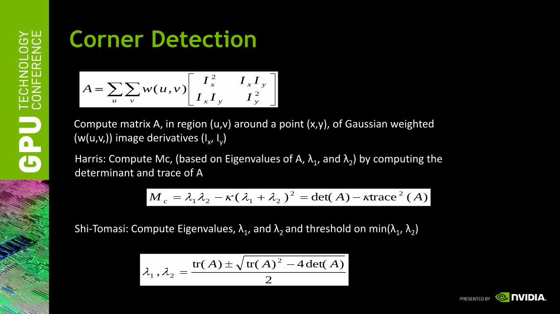
Corner Detection

u v yyx

yxx

III

IIIvuwA

2

2

),(

)(trace)det()( 22

2121 AAM c

Compute matrix A, in region (u,v) around a point (x,y), of Gaussian weighted (w(u,v,)) image derivatives (Ix, Iy)

Harris: Compute Mc, (based on Eigenvalues of A, λ1, and λ2) by computing the determinant and trace of A

2

)det(4)tr()tr(,

2

21

AAA

Shi-Tomasi: Compute Eigenvalues, λ1, and λ2 and threshold on min(λ1, λ2)

Feature Detection

Shi-Tomasi + Non-maximal Suppression

Corner Detection @ 1024x768

GPUs vs Intel E5440 CPU

0 10 20 30 40 50

GPU C1060 (2.3 ms)

GPU Quadro 570m(12.4 ms)

CPU (47.2 ms)

Time (ms)

Compute Derivatives & Eigenvalues Compact Eigenvalues Non-maximal Suppression Generate Points

Corner Detection

Weak Threshold Strong Threshold

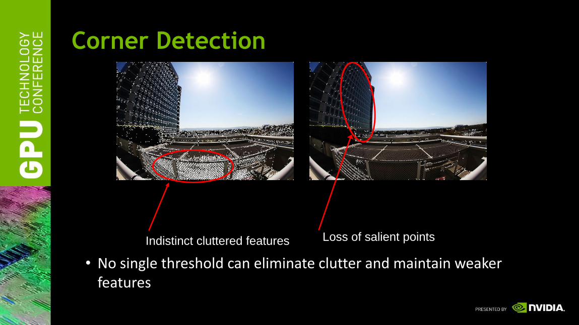
• No single threshold can eliminate clutter and maintain weaker features

Corner Detection

Weak Threshold Strong Threshold

• No single threshold can eliminate clutter and maintain weaker features

Indistinct cluttered features

Corner Detection

Weak Threshold Strong Threshold

• No single threshold can eliminate clutter and maintain weaker features

Indistinct cluttered features Loss of salient points

Modified Shi-Tomasi

• Take ratio of min(λ1, λ2) to its

neighbourhood

• Reduces clutter, maintains

distinctive (though weaker) features

Dynamic Threshold

Corner Detection: Dynamic Method

u v yyx

yxx

III

IIIvuwA

2

2

),(

2

)det(4)tr()tr(,

2

21

AAA

Dynamic Thresholding: Compute Eigenvalues

u v

rM),min(

),min(

21

21

Dynamic Threshold: Compare min(λ1, λ2) to regional (u,v) minimum

Compute matrix A, in region (u,v) around a point (x,y), of Gaussian weighted (w(u,v,)) image derivatives (Ix, Iy)

Additional Computational Cost: One 2D convolution and a division/comparison

Dynamic Feature Detection

Dynamic Thresholding Corner Detection @ 1024x768

GPUs vs Intel E5440 CPU

0 10 20 30 40 50 60

GPU C1060 (2.7 ms)

GPU Quadro 570m

(15.4 ms)

CPU (56.2 ms)

Time (ms)

Compute Derivatives & Eigenvalues Compact EigenvaluesNon-maximal Suppression Generate Points Dynamic Threshold

Pixels to Points: HistoPyramids

• How to go from pixels to ( x,y ) point coordinates, on the GPU?

(0,0)

(24,20)

(48,20)

(124,30)

(148, 44)

(24,45)

(56, 48)

(347,569)

(271,756)

(273,881)

…

GPU HistoPyramids

• Based on papers by Ziegler et al. (NVIDIA)

• Able to generate a list of feature coordinates completely on the

GPU

• Determines:

– What is the location of each point?

– How many points are found?

• Applicable for quadtree data structures

Gernot Ziegler, Art Tevs, Christian Theobalt, Hans-Peter Seidel, GPU Point List Generation through HistogramPyramids

Technical Report, June 2006

See http:// www.mpii.de/~gziegler for full information

HistoPyramids• How do we generate a list of points on the GPU from an image

buffer containing 1’s (points) and 0’s (non-points)

• Do a reduction: each level is the sum of 2x2 region “below” it

• The top level is the number of points total

1 0 1 0

0 01 0

0 00 0

1 0 1 0

0 01 0

0 00 0

0 10 0 0 10 1

0 01 0 0 10 1

0 00 1 0 10 1

0 00 0 0 00 1

0 00 0 0 00 1

HistoPyramids• How do we generate a list of points on the GPU from an image

buffer containing 1’s (points) and 0’s (non-points)

• Do a reduction: each level is the sum of 2x2 region “below” it

• The top level is the number of points total

1 0 1 0

0 01 0

0 00 0

1 0 1 0

0 01 0

0 00 0

0 10 0 0 10 1

0 01 0 0 10 1

0 00 1 0 10 1

0 00 0 0 00 1

0 00 0 0 00 1

1 0

0 1

2 1 2 1

0 01 2

1 01 4

0 00 2

HistoPyramids• How do we generate a list of points on the GPU from an image

buffer containing 1’s (points) and 0’s (non-points)

• Do a reduction: each level is the sum of 2x2 region “below” it

• The top level is the number of points total

1 0 1 0

0 01 0

0 00 0

1 0 1 0

0 01 0

0 00 0

0 10 0 0 10 1

0 01 0 0 10 1

0 00 1 0 10 1

0 00 0 0 00 1

0 00 0 0 00 1

1 0

0 1

2 1 2 1

0 01 2

1 01 4

0 00 2

2 1

0 1

4 5

2 6

HistoPyramids• How do we generate a list of points on the GPU from an image

buffer containing 1’s (points) and 0’s (non-points)

• Do a reduction: each level is the sum of 2x2 region “below” it

• The top level is the number of points total

1 0 1 0

0 01 0

0 00 0

1 0 1 0

0 01 0

0 00 0

0 10 0 0 10 1

0 01 0 0 10 1

0 00 1 0 10 1

0 00 0 0 00 1

0 00 0 0 00 1

1 0

0 1

2 1 2 1

0 01 2

1 01 4

0 00 2

2 1

0 1

4 5

2 6

4 5

2 6

17

HistoPyramid

• The pyramid is now a map to where the point locations are

• Traverse down the pyramid, counting past points, and populate the list

• Example: at what coordinates is the 5th point in the list

Time: (C1060 GPU)1024x1024: 0.27 ms4096x4096: 2.1 ms8192x8192: 7.7 ms

1 0 1 0

0 01 0

0 00 0

0 1 0

0 01 0

0 00 0

0 10 0 0 10 1

0 01 0 0 10 1

0 00 1 0 10 1

0 00 0 0 00 1

2 1 1

0 01 2

1 01 4

0 00 2

0 00 0 0 00 1

4

2 6

17

Holds points 1..4

Holds points 5..9:

Point 5 must be inside

(below) this quadrant

Holds Points 5,6: point 5 must

be inside this quadrant

This must be point 5

1 2 5

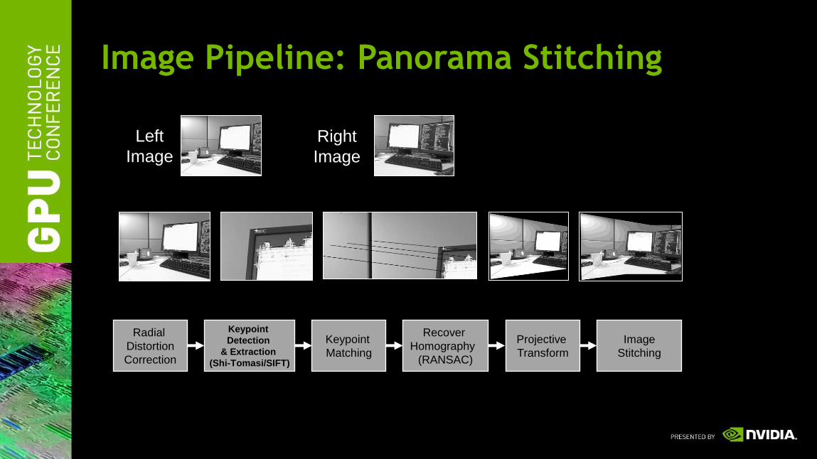
Image Pipeline: Panorama Stitching

Keypoint

Detection

& Extraction

(Shi-Tomasi/SIFT)

Keypoint

Matching

Recover

Homography

(RANSAC)

Projective

Transform

Image

Stitching

Left

Image

Right

Image

Radial

Distortion

Correction

Generating Descriptors

• What’s a Feature Descriptor?

– Distinct numerical representation of an image point for

matching

• Our example: SIFT

– “Scale Invariant Feature Transform”

– 128 element floating point vector (“key”)

– Nearest Euclidean distance between keys is the best match

Lowe, David G. (2004). "Distinctive Image Features from Scale-Invariant Keypoints". International Journal of Computer Vision 60 (2): 91–110.

Generating Descriptors

• Sparse point processing

• HistoPyramid tree organization gives good spatial locality!

• Parallel processing of single descriptor with thread cooperation

– Shared Memory

– Thread Synchronization

1. Calculate feature

orientation (shared

memory reduction)

2. Lookup rotated samples

(texture cache)

• Made possible by Thread Cooperation and data dependent array

indexing in compute shaders

• Good texture cache usage, constant cache (Gaussian weights)

Thread

Processors

Shared

Memory

Double

Multiprocessor

Feature Descriptor Computation

Feature Descriptor Computation

1. Calculate feature

orientation (shared

memory reduction)

2. Lookup rotated samples

(texture cache)

3. Generate local

orientation histograms

(one thread per

histogram,shared memory,

pointer indexing)

• Made possible by Thread Cooperation and data dependent array

indexing in compute shaders

• Good texture cache usage, constant cache (Gaussian weights)

Feature Descriptor Computation

1. Calculate feature

orientation (shared

memory reduction)

2. Lookup rotated samples

(texture cache)

0.031714 0.087833 0.027565

0.000000 0.005982 0.115469

0.132375 0.026356 …

3. Generate local

orientation histograms

(one thread per

histogram,shared memory,

pointer indexing)

• Made possible by Thread Cooperation and data dependent array

indexing in compute shaders

• Good texture cache usage, constant cache (Gaussian weights)

4. Normalize Histogram

(shared memory reduction)

5. Threshold

6. Re-normalize Histogram (shared

memory reduction)

Matching Results

Image Pipeline: Panorama Stitching

Keypoint

Detection

& Extraction

(Shi-Tomasi/SIFT)

Keypoint

Matching

Recover

Homography

(RANSAC)

Projective

Transform

Image

Stitching

Left

Image

Right

Image

Radial

Distortion

Correction

Blending can cause artifacts

Better: Image Stitching

Binary Labeling

Pixels from Image A

Pixels from Image B

Seam

What defines a good seam?

Intuition: Must not be noticeable

— Avoid introducing new gradients

Breaking it down on the pixel level:

— Color differences between pixels of images should be minimal at

seam pixels

Image A Image B

Computing good seams

p q p q

Image A Image B

p q

22)()()()( qIqIpIpIC BABA

Markov Random Field

Computing good seams

Graph Cut to compute the minimal cost seam

— Very fast, global optimal solver for binary label problems

— NPP primitive (upcoming 3.2 release)

Best seam is the Minimum Cut

NPP Graphcut

Graph is stored in Arrays

— Weights to terminals in one array

— Weights to neighbors in four arrays, horizontal edges are

transposed

nppiGraphcut_32s8u(d_terminals, d_left_transposed, d_right_transposed,

d_top, d_bottom, step, transposed_step, size,

d_labels, label_step, pBuffer);

Binary Labeling

Pixels from Image A

Pixels from Image B

Seam

From two images to many

One label for each image in the set: N labels

— Assign each pixel in the panorama one label

— Unfortunately this is NP hard problem

Alpha-Expansion algorithm to the rescue

— Intuition: “Keep current label or change to alpha”

— Again binary problem solvable with Graph Cut

— Repeat for all labels until the optimal solution is found

Alpha-Expansion

Iteration for each label alpha:

— Compute data term for alpha

— Compute neighborhood terms for alpha

— Solve binary Graph Cut

— Use binary solution to get expanded multi-label solution

— Compute total energy of expanded solution

— If energy has decreased make this the current solution, otherwise

discard

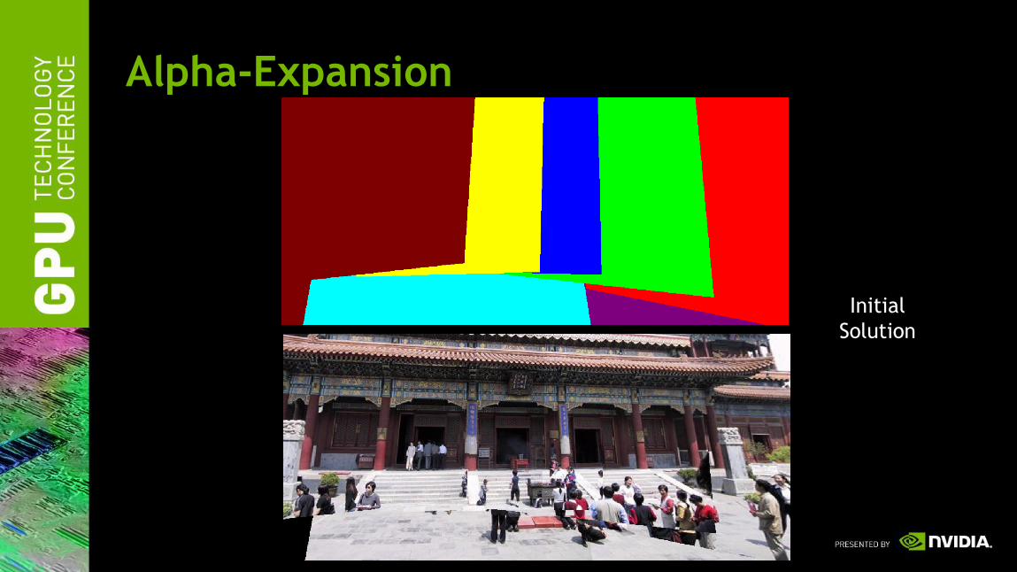
Alpha-Expansion

Initial

Solution

Alpha-Expansion

After 6

Expansion

Steps

Alpha-Expansion

After 12

Expansion

Steps

Alpha-Expansion

After 18

Expansion

Steps

Final Result

Image Stitching Notes

In this example only 6 out of the 7 input images contribute

to the final result

— Image Stitching reduces the image set

Quality improves with each iteration

— The current result is a preview that converges to the final result

PerformanceTest data set

Image 0 Image 1

Performance

CUDA 3.0, Driver 260.16 wall clock times

Iteration Time (ms)

GTX460 GTX 480

1 101.74 50.44

2 102.85 50.77

3 31.95 18.95

4 28.59 18.68

5 28.18 18.82

6 28.92 18.59

Alpha Expansion Performance

Image Pipeline: Panorama Stitching

Keypoint

Detection

& Extraction

(Shi-Tomasi/SIFT)

Keypoint

Matching

Recover

Homography

(RANSAC)

Projective

Transform

Image

Stitching

Left

Image

Right

Image

Radial

Distortion

Correction

Example Application

Questions?