Fast Elliptic Solvers and Three-Dimensional Fluid-Structure

JOURNAL OF COMPUTATIONAL PHYSICS 36, 93-127 (1980)

Fast Elliptic Solvers and Three-Dimensional Fluid-Structure

Interactions in a Pressurized Water Reactor

U. SCHUMANN

Kernfoschungszentrum Karlsruhe, Institut fiit Reaktorentwicklung, Projekt Nukleare Sicherheit, Karlsruhe, Federal Republic of Germany

Received September 28, 1978; revised August 9, 1979

A numerical method is described for analysis of the response of internal structures in the vessel of a pressurized water reactor to a sudden depressurization (“blowdown”). The three-dimensional geometry and fluid-structure interactions are taken into account. Potential flow is assumed for a compressible fluid with constant speed of sound which is appropriate for subcooled water. Any linear-elastic dynamic model in terms of a finite number of degrees of freedom can be employed for the internal structure, in particular the core barrel; here the model “CYLDYZ” is implemented. An implicit and stable time- differencing scheme is used. Spatially, finite differences or spectral approximations are introduced. The resultant set of linear equations is solved efficiently by means of fast elliptic solvers and the capacitance, or influence, matrix technique. The resultant code, FLUXZ, is applied to predict the dynamics in case of the planned HDR experiment. A sensitivity analysis shows that truncation errors can be kept sufficiently small. By comparison of results with and without fluid-structure interactions it is found that the coupling has an essentiaf effect on the resultant maximum stress.

Contents. 1. Introduction. 2. The Basic Equations. 3. Time Discretization. 4. Space Discretization. 5. Solution Method. 6. Numerical Results. 7. Discussion. Appendix: Discussion of Model Assumptions. Nomenclature.

1. INTRODUCTION

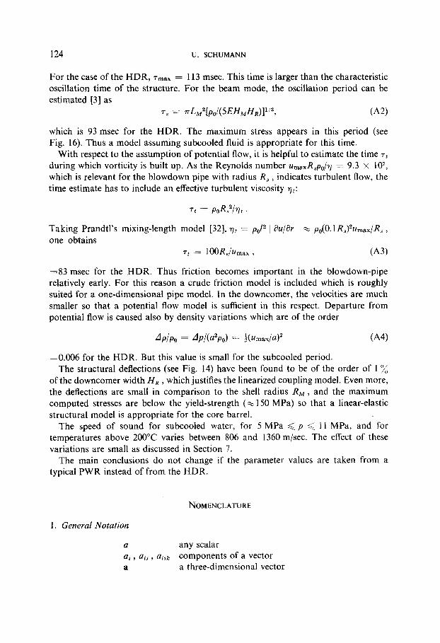
A sudden break of one of the pipes through which the coolant is fed into the vessel of a pressurized water reactor (PWR) would cause a rapid depressurization and blowdown of the initially subcooled water inside the vessel. The transient pressure field imposes large forces on the vessel’s internal structures. In particuIar the core barrel (see Fig. 1) must resist these loadings so that normal shutdown and emergency cooling of the core (not shown in Fig. 1) remain possible. It will be shown that for realistic evaluation of the core barrel deformations one has to account for the fluid- structure interactions. In this paper a numerical method is described that simul- taneously computes the fluid and core barrel motion. The method has been implemented in a PL/I computer code named FLUX2.

Because of the three-dimensional geometry and the coupIed motion, such a simulation is expected to require a very large amount of computing time unless

93 0021-9991/80/070093-35$02.00/O

Copyright 0 1980 by Academic Press, Inc. All rights of reproduction in any form reserved.

94 U. SCHUMANN

b c d Failure Close to the lnlel Nozzle of the Primary Ccdont Circuit

.:<f’.’ .: _’ 1,‘. Zone of *’ . Reduced Pressure

FIG. 1. Schematic picture of the depressurization and deformation sequence [5].

suitable simplifications and efficient numerical methods are employed. It will be shown that sufficient accuracy is obtained for time steps which are much larger (10 to 20 times) than those required for stability in an explicit scheme. An implicit and stable time integration scheme will be described which requires only about twice the computing time of an explicit scheme. Therefore, the implicit scheme is more efficient than an explicit one. Also, an implicit scheme allows to treat incompressible fluid flows as well as compressible ones.

In an implicit scheme, the main computing time is spent in solving the resultant set of equations at each time step. If the fluid model is chosen properly, the set of equations for the flow variables has the form of Helmholtz’ equation

div gradp - h2p = q. (1)

On a rectangle with boundary conditions of constant type along each side, this is a separable elliptic partial differential equation. On a regular rectangular mesh and with second-order finite differences, the resultant set of linear equations is of a form which can be treated directly and very efficiently by means of a “fast elliptic solver” [ 11. For specific problems fast elliptic solvers have been shown to perform typically 50 times faster than standard iterative methods [l]. On irregularly shaped regions fast elliptic solvers can be employed by means of an “influence matrix technique” (com- monly termed “capacitance matrix technique”) [l, 21. In the present context the influence matrix technique (IMT) is used not only to account for geometrical irre- gularities but also for the coupling to the structural equations.

In order to achieve the type of partial differential equations amenable to the direct solution scheme, the fluid motion is modeled as compressible potential flow with constant velocity of sound. The assumption of potential flow reduces mainly the storage requirements because the scalar potential variable replaces three velocity components as integration variables. The nonlinearity represented by the kinetic

FLUID-STRUCTURE INTERACTIONS 95

energy of the fluid, which is of great physical importance [3, p. 1.51, is not neglected. Because of this nonlinearity, at each time step a separate Poisson equation (Eq. (1) with h2 = 0) is to be solved. For this purpose the method used for the implicit pressure equation can be used as well. Otherwise the fluid is treated as an acoustical medium. Such a model is appropriate for the subcooled flow regime in the initial part of the blowdown (typically up to 100 msec) in which the largest structural deformations appear. The flow boundaries are rigid walls except for the core barrel, which is approximated as a thin linear-elastic cylindrical shell. The dynamics of this shell are described at present by the CYLDY2 model [4], which is based on Fliigge’s shell equations using analytical form functions and a variational principle. Coupling is accounted for with respect to the pressure loads on the structure and the normal shell velocities defining the flow boundary conditions at the (undeformed) interface.

Until recently the state of the art [5] approach for analysis of the structural deformations was such that the pressure field was calculated for rigid structures and the reaction of the structures was determined subsequently. This “decoupled” analysis procedure does not take into account the reduction of pressure differences due to alterations of flow volumes. Also it does not account for the enhanced effective mass of the coupled fluid-structure system so that the reaction to load peaks is over- estimated. Finally the decoupled analysis implies that energy is transferred from the fluid to the structure but not vice versa. As a consequence, in cases where the frequency of the imposed oscillating fluid load is close to one of the several eigenfrequencies of the structure and the loading is applied for sufficiently many cycles, the amplitudes of the structural oscillations can grow virtually without limits unless a damping process (which is hard to define properly) is included. Therefore, the decoupled analysis is liable to overestimate the structural response. In physics, however, there are no oscillating external forces imposed on the coupled system other than the sudden break, which essentially causes a step-load for which the dynamical response is finite. So, the resonance problem is peculiar to the decoupled analysis and not at all relevant to the real physical behavior.

At present, several groups are developing coupling analysis tools for this problem and preliminary results have been published [6-141. In some cases only the virtual fluid mass tis taken into account [lo, 121. Others resolve the fluid motion in the downcomer (see Fig. 1) only, for which “2~-dimensional” models are in use [8, 91. A three-dimensional model which accounts for two-phase flow properties has been developed at Los Alamos [13]. These methods are all based on iterative solution schemes. Taking the iterative method implemented in the “2&dimensional” code STRUYA [9] for reference, the present three-dimensional method has been found to be about 50 times faster [14].

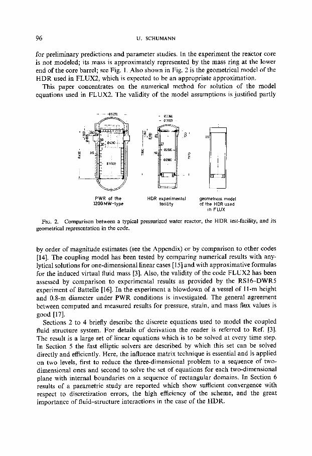
The present investigation forms part of a more extended experimental and theoretical program in which the former HDR reactor is used as a test facility [5]. Figure 2 shows the test configuration in comparison to a commercial PWR of the 12O&MW size. The HDR-blowdown experiments are planned to be run in 1980/1981. The results will be used to verify the present and several of the above-mentioned codes and to compare their accuracy and efficiency. Here, the data of the HDR facility are used

96 U. SCHUMANN

for preliminary predictions and parameter studies. In the experiment the reactor core is not modeled; its mass is approximately represented by the mass ring at the lower end of the core barrel; see Fig. 1. Also shown in Fig. 2 is the geometrical model of the HDR used in FLUX2, which is expected to be an appropriate approximation.

This paper concentrates on the numerical method for solution of the model equations used in FLUX2. The validity of the model assumptions is justified partly

PWR of the 1200 MW-type

HDR experimental facility

geometrical model of the HDR used

in FLUX

FIG. 2. Comparison between a typical pressurized water reactor, the HDR test-facility, and its geometrical representation in the code.

by order of magnitude estimates (see the Appendix) or by comparison to other codes [14]. The coupling model has been tested by comparing numerical results with any- lytical solutions for one-dimensional linear cases [15] and with approximative formulas for the induced virtual fluid mass [3]. Also, the validity of the code FLUX2 has been assessed by comparison to experimental results as provided by the RSi6-DWR5 experiment of Battelle [16]. In the experiment a blowdown of a vessel of 1 l-m height and 0.8-m diameter under PWR conditions is investigated. The general agreement between computed and measured results for pressure, strain, and mass flux values is good [17].

Sections 2 to 4 briefly describe the discrete equations used to model the coupled fluid-structure system. For details of derivation the reader is referred to Ref. [3]. The result is a large set of linear equations which is to be solved at every time step. In Section 5 the fast elliptic solvers are described by which this set can be solved directly and efficiently. Here, the influence matrix technique is essential and is applied on two levels, first to reduce the three-dimensional problem to a sequence of two- dimensional ones and second to solve the set of equations for each two-dimensional plane with internal boundaries on a sequence of rectangular domains. In Section 6 results of a parametric study are reported which show sufficient convergence with respect to discretization errors, the high efficiency of the scheme, and the great importance of fluid-structure interactions in the case of the HDR.


2. THE BASIC EQUATIONS

2.1. Fluid

We assume:

potential flow (symbols are defined under Nomenclature)

u = grad @. (2)

a bulk friction force per unit volume as given by -KU, where K is an empirical coefficient. (By means of this model friction in the blowdown-pipe, which has been found to be important by comparison to an experiment [ 171, can be roughly accounted for. Such a friction force is irrotational and thus consistent with the assumption of potential flow as long as K is constant.)

an equation of state of the form

(P -Pu) = U2(P - PO).

with constant speed of sound a.

(3)

small Mach numbers so that (u~~~/czz)~ < 1.

With these assumptions Euler’s momentum equation and the continuity equation result [3, Sect. Al] in a wave equation for the pressure p

f (j + ~b) - div gradp = div grad E; 1

E == z pou2. (4)

The rate of change @ of the potential is also determined by Euler’s equation, the divergence of which can be expressed as

div grad I,!I = 3 ($ t Kj) (3

with an auxiliary potential

2.2. Structure

The deformation w(x, t) of the linear-elastic structure can be assumed to be expressible by

w(x, t> = v(&>, x> (7)

in terms of a finite and holonomic [18, p. 401 set of modes c = {ci} (“generalized coordinates” [lS, p. 391). From Lagrange’s equation of motion one gets the dynamical equations [18, pp. 45, 1571

Mr: + D-i + SC = q, (8)

98 U. SCHUMANN

where M, D, and S are the mass, damping, and stiffness matrices, respectively, and v = (qi) the modal forces due to the pressure acting in the direction n normal to the structure integrated over the surface 0:

(9)

The details of v, M, and S are taken from the CYLDY2 model developed by Ludwig and Krieg [4]. In this model the core barrel is treated as a thin linear-elastic cylindrical shell, clamped at the upper end and attached to a rigid mass ring at the lower end. According to the symmetry with respect to the angle y = 0 the three components of the displacement w at the axial position z and angle 9 are expressed as

F$‘(z) cos(ncp) &,(f)

w(z, cp’, t) = 5 : F;‘(z) sin(ny) ci$l(t) tz=o m=l

F;;)(z) cos(mp) &f(t)

The notation ci?y) is an alternative to ci and accounts for the natural ordering with respect to azimuthal (n = 0, I,..., N) and axial (m = 1, 2 ,..., M) modes. The axial form functions F:‘(z) (F’ = dF/dz) are taken as the eigensolutions of a vibrating beam. Because of the axial symmetry of the structure, M and S consist of block matrices M,,I, and S,,, which are nonzero on the diagonal (n = k) only. This property is of high importance with respect to the efficiency of CYLDY2 and FLUX2.

In FLUX2 a principal axis transformation

c = X6 (11)

is used, where the eigenvector matrix X and eigenvalue matrix A are defined by

-MXA + SX = 0. (12)

This eigenvalue problem is split into (N + 1) smaller problems for each azimuthal mode because of the block-diagonal form of M and S.

The principal axis transformation results in a set of structural equations with diagonalized matrices (unit matrix instead of M, eigenvalue matrix A instead of S):

ji + Qb’ .r a/; 7= ), (13)

> = A(XrSX)--’ Xrr/. (14)

The damping matrix is defined according to common practice [18] so that 0 is a diagonal matrix:

0 = diag(P), A = diag(h’i)), (15)

&I = &‘i’ tlMUPJ(7)’ &i) = (^w)l;%,


The parameter s$&, is the equivalent viscous modal damping ratio for the ith mode [19] and must be specified empirically. Structural damping is included in order to make parameter studies and adaption to experiments possible. In the integration scheme structural modes with eigenfrequencies wCi) above an input value wmas (q2n/dt) are neglected.

2.3. Boundary and Coupling Conditions

At walls the normal velocities and accelerations are set equal. This implies

n * (ti + KU) = n . grad 4 = n . (ti + ~ti) (16)

and because of Euler’s equation

n . grad(p $ f?) = -pun . (% f Kti). (17)

For the kinetic energy per unit volume we use

n . grad E = 0 iw

at all boundaries (which is exact at rigid walls). Such a boundary condition is required because for the structural loads we must know p alone whereas in the fluid (p A- E) is the relevant unknown. The correct condition n . grad E = p,n + [(grad @ . 0) grad @] would require one-sided difference approximations. The errors introduced by the approximation (18) are small as long as the normal wall velocities are small in comparison to the tangential ones in the fluid.

At openings one can either prescribe the pressure p = pF(t) or the normal velocity. Here, the former is specified in the form

Pdt) = PO + (PI - Po)f(t/dtbreakh 0 < f < ~tbreak ,

(19) = p1 1 t > dtbreak ,

where d tbreak is a measure of the break opening time and f(T) an appropriately chosen function, e.g., a ramp (J(T) = &(T) ~~7 T) or a trigonometrical function (f(7) = &(T) L sin2(Tn/2)). As the present model cannot account for two-phase flow effects explicitly, the value p1 is set equal to the local saturation pressure. This is known to be appropriate according to two-phase fluid models [14].

When the pressure field has been determined according to this boundary condition the velocity potential must satisfy the condition

n . grad 4 = -(l/pJn . grad p

as a consequence of Euler’s equation and Eq. (18).

100 U. SCHUMANN

It is easy to verify that the following integral relations are satisfied as required for consistency.

jjj f (2; + '$'I dV = jjj div grad(p + E) dV = - j/j p,, div grad 4 0 V V V

= -4 . n . grad(p -i- E) dS = fJ’ p,,n * grad # dS. (20)

2.4. Initial Values

It is assumed that the fluid and structure are at rest initially, so that at time t = 0 we start with

(P, 9, @, w, 3 = (PO , 0, 0, 0, O),

although other initial values which satisfy the interface and consistency conditions are possible as well.

3. TIME DISCRETIZATION

One can view the given set of equations for the structural modes 8 and the pressurep as one dynamical equation for the unknowns J = (6, p(x))’

M’Z + D’; A S’s = ?/(@(t),pF(t)) (21)

with suitable operators M’, D’, and S’. The right-hand side (r.h.s.) 1/ is a nonlinear function of the potential CD (due to the kinetic energy) and a linear function of the prescribed boundary value pF(t).

For numerical integration of such equations the well-known Newmark method [20] can be used, which is constructed as follows. The time ordinate is divided into equidistant time steps tn x n At for which .ln approximates .j(t”). Then we substitute

:j := (I/op)(.J~~l - 2.,‘” j- J”-l), (224

> := (1/2Llt)(.p-l ~ .,,c-y, Wb)

1 :- p.,n-1 + (I - 2/3) .,n J- p.w. (224

For /3 > 0, this results in an implicit scheme with respect to ~+-l. On the r.h.s. the nonlinear part is treated explicitly:

Y(W), pdt)) : = y(@(t “), @PPF(tn-: ‘) $ (I ~ 2p) p#) + &,(t “+‘)). (23)

The Newmark scheme is second-order accurate, free of damping, and (for the linear case with neglected kinetic energy) unconditionally stable if 2 < /3 -< 4


[20; 3, Sect. A2]. We use j3 = $ in the integrations. No instabilities due to the explicitly treated kinetic energy have been encountered.

Once the new pressure value pn~+l is known, one can integrate Eq. (5) and compute the new potent.ial @+l 3 @(t %+I) from Eq. (6) in discrete form:

This scheme is again unconditionally stable in the linear case but only first-order accurate. Its reduced accuracy is tolerable because it influences the solution vector 5 by means of the kinetic energy only.

In order to proceed from one time step to the next, one has to solve the implicit equations for 8+l and thence for $. In both cases this involves a Helmholtz equation for the fluid variables; see Eq. (1). The Helmholtz parameter h2 is

h2 = (1 + K dt/2)/(/%? dt’) (25)

in case of the pressure, and zero in case of the potential so that in the second case essentially a Poisson equation [I] has to be solved. As a result of time discretization the solution of the hyperbolic wave equation (4) for the pressure in space and time is obtained from a sequence of elliptic equations in space and thus becomes tractable by fast elliptic solvers.

4. SPACE DISCRETIZATION

Spatial discretization has to be introduced with respect to the Helmhoitz equations for the pressure and the potential (we concentrate on the former from now on) and for the coupling to the structure. Because of the complex geometry, the details (as given in [3]) are very lengthy to write up and not given here.

4.1. Partitioning into Vessel and Pipe Domains

Whereas the vessel domain has to be treated as strictly three-dimensional (3D), a one-dimensional (1D) approximation suffices for the broken pipe. This has been suggested by comparing 1D and 2D potential flow solutions for incompressible fluid flow in the nozzle [21] as well as results of 1D and 2D computations for this domain with the two-phase flow analysis code DRIX-2D [14]. Accordingly, the fluid domain is subdivided as sketched in Fig. 3. The vessel solution is termed p(x) = p(r, z, v), the pipe solution is p(x) = ps(v). In order to have Neumann boundary conditions at the vessel boundary everywhere, the interface condition will be formulated in terms of the normal gradient g, = n . grad p at the interface and the surface mean pressure pD at the nozzle.

102 U. SCHUMANN

-P’P,

FIG. 3. Partitioning into vessel and pipe domain.

4.2. Separation into a Set of Two-Dimensional Problems

If the interface value g, were known, the remaining 3D “vessel problem” could be separated by means of a cosine transformation into a set of separated 2D Helmholtz equations. This is possible for the following reasons: linearity of the equations, axisymmetry of the geometry, angular independence of the type of boundary conditions (Neumann boundary condition at the vessel wall and at the nozzle), and the planar symmetry of the boundary values with respect to the angle y = 0. The discrete cosine transform of Eq. (1) is

where hn2 = n2 if the azimuthal derivatives are approximated according to the Fourier approximation and h, 2 = ~(N/T)~ [l - cos(nrr/lv)] if second-order finite differences are used (usually we use the former). The carets denote cosine series coefficients (jn = $Jz, r)).

4.3. Spatial Discretization of the 20 and 1 D Problems

The r-z planes of the vessel are covered by a grid as plotted in Fig. 4. The grid is regular (unlike the grids which would be used in finite-element approximations) in order to allow for application of fast elliptic solvers. The grid lines by construction coincide with boundary lines. The symmetry line forms the middle of the first column of cells. The cell mean pressure value pijk is assigned to the cell midpoint as on a staggered grid (see Fig. 5).

By means of Gauss’ integral theorem one obtains a relation between the mesh mean values and the average normal gradients at the cell boundaries. In the inner fluid domain, the gradients are approximated by second-order finite differences in terms of the values pijk in the adjacent cells. At boundaries, however, the normal gradients are either known (e.g., zero at rigid walls) or expressible in terms of normal structural accelerations; see Section 4.5.

The ID Helmholtz equation for the pipe domain is even simpler and is approximated in an analogous manner.


i- lt.l&43 MM MV Mvs

0 1 2 3L56-78 9 10 11 12

h '1 12 !----MS-.---

I rlt2 rl + 112.

t 2 I

3 1

N,=l, ’

5 ’

6

NL=12

--1 - -ALv~ for irh.i

X Pijk

A Ps,i

Q irregular cell , 2D

A irregular cell ,30

Ftc;. 4. The mesh grid.

Uzrdj+l/2)k +

a pm+ ur,(i*l/Z)jk

i, r-9 1 Pljk

FIG. 5. The variables as allocated on a staggered grid cell.

104 U. SCHUMANN

4.4. Interface Condition at the Nozzle

At the nozzle one or several mesh cells (z&) with i = M, (see Fig. 4) of the vessel are in contact with the pipe cross section. Let us define a coefficient oljlc expressing the ratio of this contact area to the outer surface area Rydy dzj of the vessel cells. As illustrated in Fig. 6, the cross section of the “pipe” may be arbitrarily shaped, so that, e.g., a slit in the vessel can be treated as well as a circular pipe. With this defi- nition, the normal gradient g, in the cell (ijk) attaching the interface is expressed by finite differences as follows:

The variable pS,i+I is the first discrete value in the pipe. The gradient gv,j, can be used to account for a flexible vessel wall but is set to zero here.

j-1

I j

tz k-0 -k

FIG. 6. Example of possible unconventional pipe cross section; the quantities oljlr equal the frac- tion of individual mesh cell areas in contact with the pipe cross section.

The boundary value p. used for the pipe is consistently expressed by a weighted mean of the discrete values in the vessel-mesh-cells adjacent to the nozzle:

PD = i c %Pijlc i == /WV. (28)

If a 2D or 3D grid should be used for the pipe, the interface conditions could be generalized in a straightforward manner.

4.5. The Spatially Discretized Structural Deformations

The core barrel is in contact with the fluid for NF fluid cells in each azimuthal plane (see Fig. 7). We denote these cells by indices (jk), ,j = 1, 2 ,..., NF ; k = 0, I,..., N. In the program we make use of the fact that the core barrel is treated as a thin shell and the mass ring is rigid so that the normal deformations are equal on both sides of the structure.


I

FIG. 7. Numbering of the contact surface cells between core barrel and fluid region.

For the coupling, one has to relate the normal structural deformation w, :e n ’ w (or acceleration) to the normal gradients gW CC= n . grad p at the walls. For each mesh cell (,~k) we set

w, jk = n . V(c, (Zj , yk)) 3 Vj,L,nC, , (29)

i.e., we use the structural deformation in the middle of the cell. Perhaps one should use the mean value of II . v in the cell area in order to be consistent with the gradients, which are defined as such mean values. However, this would inhibit easy exchange of different structural models with different form functions V(C, x). In obvious matrix notation one can formulate Eq. (29) as

Cl’ ,l Y- vr -z 56, 5 :I vx.

4.6. The Structural Loads Due to the Discrete Pressure Field

Equation (9), defining the structural loads qm , can be approximated by

(30)

where use has been made of Eq. (29) and Ojk is the contact surface of the mesh cell (jk) and pu.,jk is a discrete representation of the wall pressure. This wall pressure is computed from the pressure pijri in the middle of the wall adjacent cell and a correction by means of the normal gradient g,c,jk at the wall and the normal distance AX,, to the mesh midpoint:

Pv,jl; = PL~JC - Sm,zi; Axjk . (32)

106

The result

U. SCHUMANN

can be expressed in matrix notation by

y= -(R/c - R’y,)

and the transformed loads 1 according to Eq. (14) are, e.g.,

i == (R/2 - l+),

a = A(XTSX)-l XTR.

(33)

(34)

(35)

4.7. Symbolic Representation of‘ the Equation System

Without going into the details it can be seen that the resultant equations are of the form

I 0 0 G, G,

--__ --

0 0 0 D L.7

(36)

The first line of this matrix equation expresses the interface condition, Eq. (27), between the normal gradient yD and the pressure values /Z and jS in the vessel and the pipe. I is a unit matrix. GD and G, contain only as many nonzero lines as there are vessel-grid-cells in contact with the pipe.

The second line is a consequence of the time-discretized structural equation (13). K stems from the mass, damping, and stiffness matrices according to the implicit scheme, 8’ and i? account for the loadings in terms of the gradients at the wall, c/?,. , and the pressure /I in the vessel.

The third line represents the structure-fluid boundary condition, Eq. (17), after introducing time discretization and after spatial discretization as defined in Eq. (30); p = poa2X2.

The fourth line contains the matrix L which is the discrete 3D Helmholtz operator acting on the discrete pressure values; W accounts for the gradients at the core barrel wall and N for the gradients at the pipe nozzle.

Finally, the fifth line represents the ID Helmholtz operator; it is a tridiagonal matrix. The relation to the vessel values according to Eq. (28) is achieved by the matrix D which is nonzero in its first line only.


The different r.h.s. vectors account for the solution values at prior time steps, for the explicitly treated kinetic energy and for the boundary value pF(t).

For the potential # a similar set of equations is to be solved, the coefficient matrix of which is obtained by deletion of the second and third lines and columns of the matrix in Eq. (36).

5. SOLUTION METHOD

5. I. The Problem and Background

In order to perform the time-integration we have to solve Eq. (36) at each time step for the new pressure and deformation values and, subsequently, a similar system for the new potential values. These systems may well comprise several thousand unknowns. Classical direct solution methods, like Gaussian elimination, would require an excessive amount of computer time and storage. Jterative schemes suffer from the fact that the matrix is not guaranteed to be diagonally dominant, in particular if the shell is light. Also the common point iteration methods, which are appropriate for diffusionlike problems, are not suited for the present problem, where “information” is transported over long distances and from one side of the wall to the other by structural motions.

Subsequently, a direct solution method is described which makes use of the given structure of the coefficient matrix and employs the following tools:

(a) fast cosine transform algorithms to evaluate discrete cosine series according to Section 4.2 [22],

(b) a fast elliptic solver (“POISTP”) for rectangular parts of the fluid region,

(c) the capacitance or influence matrix technique (IMT).

Some details concerning (b) and (c) are given below.

5.2. Tool 1: Fast Elliptic Solver POISTP

The PL/l-procedure POISTP is an extended version of the subroutines described in [23, 241. It is amenable to the solution of the set of linear equations which arises from discretization of equations of the form

on 2D rectangles using A4 grid points in the r- and N in the z-direction and either Dirichlet or Neumann boundary conditions. In case of Neumann conditions, the grid must be of staggered type. In the z-direction, equidistant grid spacings are required. The method is based on cyclic reduction. In contrast to its original Buneman version 12.51 in which (N + 1) must be equal to a power of 2 there is no such restriction on N and M. The required number of operations is of the order NM log N. In case of Helmholtz problems with large Helmholtz parameters h2 the coefficient matrix is strongly diagonally dominant. In such cases one can trade accuracy against efficiency.

108 U. SCHUMANN

At the cost of errors, which can be kept at the order of round-off errors, a truncated cyclic reduction scheme as proposed by Buzbee [26] is being used which allows reduction of the computation time typically to 30 o/o [I]. The algorithmic details are given in [3, Sect. A3].

5.3. Tool 2: The Infiruence Matrix Technique

Fast elliptic solvers like POISTP are applicable to separable problems only. On irregularly shaped regions or for boundary conditions of varying type along the sides of the rectangle, the equations are no longer separable. However, for most of the grid cells, in particular the internal ones, the finite-difference equations are still of the same form as in the regular case. So most of the, say, IZ m M x N, equations are of the same form as in the regular fast solvable case except for some m < n equations which are due to grid cells adjacent to irregular boundaries.

For such problems the TMT allows one to solve the system with an order 0(0(n) + m”) of operations, where 6(n) is the operation count of the fast solver. This well-documented technique [ 1, 2, 271 will be summarized briefly subsequently in order to define the notation.

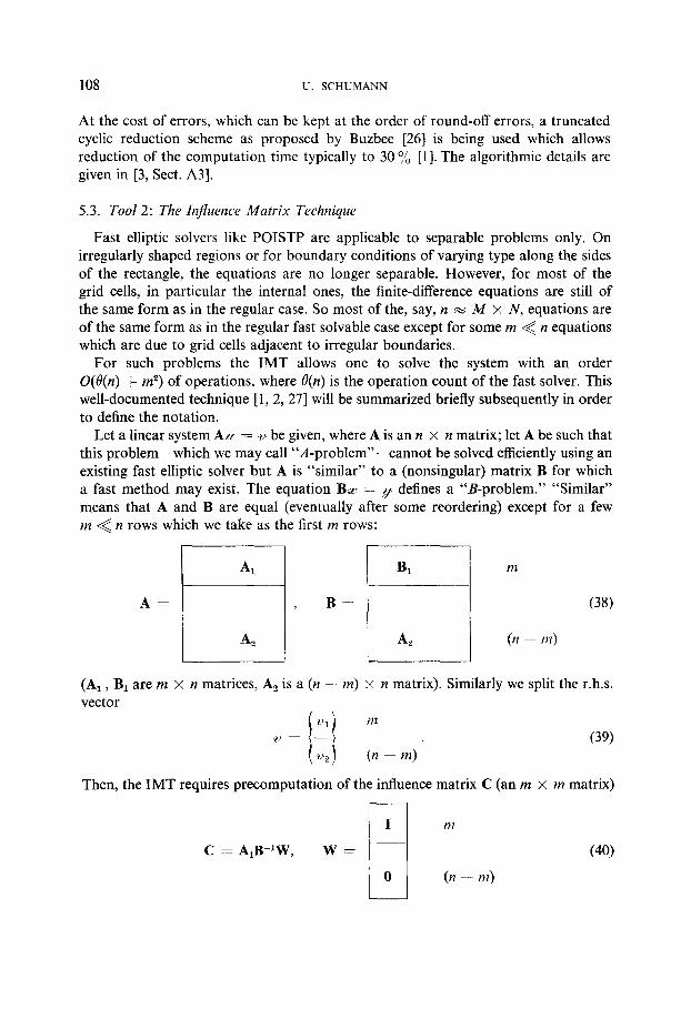
Let a linear system AU = ‘U be given, where A is an n x n matrix; let A be such that this problem-which we may call “A-problem”-cannot be solved efficiently using an existing fast elliptic solver but A is “similar” to a (nonsingular) matrix B for which a fast method may exist. The equation Bm = v defines a “B-problem.” “Similar” means that A and B are equal (eventually after some reordering) except for a few m Q n rows which we take as the first m rows:

A= B==

Bl ‘--I A2

m

(n - nt)

(38)

(A, , B1 are m x n matrices, A, is a (n - m) x n matrix). Similarly we split the r.h.s. vector

2'1

i /

172

v = - (39) u2rp (n - m)

Then, the IMT requires precomputation of the influence matrix C (an m x m matrix)

m

C = A,B-lW, w= (40)


(I = m x m unit matrix). In general C-l can be determined by solving m B-problems and performing its upper and lower triangular matrix (L- U-) decomposition [27], which requires O(me(n) + m”) operations.

The actual A-problem is solved by

(1) first solving a B-problem

B/I = 11, (41)

(2) computing the residual vector w resulting from the first m rows of the A- problem

(3) perturbing the corresponding first m components of o according to C such that the solution of

B/c = II - WC-‘w (43)

gives the desired solution IC of the A-problem.

For proof see [2, 271. Certain refinements [3] are used which will be mentioned briefly. The method can be defined also for cases where the B-problem covers more unknowns than the A-problem as is the case if the B-problem corresponds to a rectangular domain in which the irregular domain of the A-problem is embedded. If the matrices A and B are diagonally dominant then so is C and this fact can be used in a “truncated IMT” to reduce the required storage [28]. It is possible to apply this method to singular but consistent A-problems and B-problems as well [3, Sect. 4.3.31.

5.4. Application 1: Solution of the 2D Problems

The first application of these tools concerns the 2D problem which appears after cosine transformation of the 3D vessel problem as described in Section 4.2. The resultant set of equations can be written as

where the entries result from cosine transform of the corresponding entries in Eq. (36) and are all dependent on the cosine mode under consideration,

This system cannot be solved with existing fast methods because of the irregular

110 U. SCHUMANN

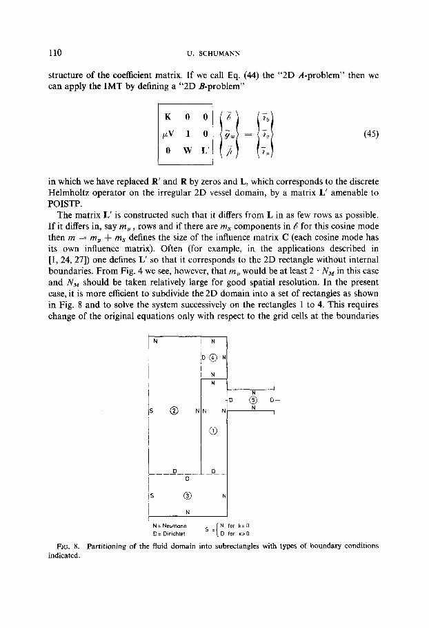
structure of the coefficient matrix. If we call Eq. (44) the “2D A-problem” then we can apply the IMT by defining a “2D B-problem”

(45)

I I

in which we have replaced R’ and R by zeros and L, which corresponds to the discrete Helmholtz operator on the irregular 2D vessel domain, by a matrix L’ amenable to POISTP.

The matrix L’ is constructed such that it differs from L in as few rows as possible. If it differs in, say m, , rows and if there are m, components in d for this cosine mode then m = m, + m, defines the size of the influence matrix C (each cosine mode has its own influence matrix). Often (for example, in the applications described in [I, 24, 271) one defines L’ so that it corresponds to the 2D rectangle without internal boundaries. From Fig. 4 we see, however, that m, would be at least 2 . NM in this case and NM should be taken relatively large for good spatial resolution. In the present case, it is more efficient to subdivide the 2D domain into a set of rectangles as shown in Fig. 8 and to solve the system successively on the rectangles 1 to 4. This requires change of the original equations only with respect to the grid cells at the boundaries

is 1 I

N z Neumann N for k: 0

D= Dirichlet 5.

D for k>O

FIG. 8. Partitioning of the fluid domain into subrectangles with types of boundary conditions indicated.

FLUID-STRUCTURE 1NTERACTIONS 111

of these rectangles as denoted in Fig. 4. In each subrectangle the remaining system corresponds to a Helmholtz problem with Neumann or Dirichlet boundary conditions as defined in Fig. 8. These systems can be solved with POISTP if dzj = const in the regions 2 and 3, respectively. The flexibility offered by POISTP with respect to boundary condition types and size of the grid is very important for this application. Another advantage of this subdivision into a sequence of rectangles is the fact that on each rectangle different values for the speed of sound can be used.

With these changes the 2D B-problem is easy to solve by successive blockwise elimination because K and I are diagonal matrices.

5.5. Application 2: Solution of the 3D Problem

After having constructed a “fast solver” for the 2D problems as described above, which by means of fast cosine transforms solves the 3D vessel problem efficiently, the total “3D A-problem” given by Eq. (36) can be solved by again applying the IMT. This problem is a fast solvable one if the matrices GD and Gs in Eq. (36) are replaced by zeros. This in fact requires the change of only a few rows of Eq. (36) because GD and Gs (as stated above) contains only as many nonzero rows as there are vessel-mesh- cells in contact with the pipe (typically 510). After this change, the solution of the first line of Eq. (36) is trivial. The second to fourth lines are solved thereafter by means of the procedure described above and the last line is treated finally by applying Gaussian elimination to the tridiagonal matrix Ls . After the second solution of this “3D B-problem” (which involves four solutions of each 2D B-problem) according to the IMT we have the result we were looking for.

This solution method gives the exact solution of Eq. (36) except for round-off errors. The round-off errors are largest for zero Helmholtz parameter and a double-precision coding has been used to ensure small errors. For large Helmholtz parameters, which are typical for the coupled pressure-deformation problem, the round-off errors are very small and allow for application of the truncated cyclic reduction scheme and the truncated IMT mentioned above.

5.6. Flow of Control in the Program

The above methods are implemented in the PLjl code FLUX2 which is structured as indicated below:

(a) Preparation. process input, define mesh grid, get structural data v, M, S, and D from a subroutine describing the structure and

perform the principal axis transformation, compute the influence matrices

(1) for the pressure and deformation for each 2D problem, for the 3D problem,

(2) same for the potential.

581/36/l-8

112 U. SCHUMANN

(b) Integration. read or set initial values, determine velocities and kinetic energy from the initial potential, loop until end of time

t := t + At, set up r.h.s. for pressure and deformation, solve 3D problem for new pressure and deformation values, set up r.h.s. for the potential, solve 3D problem for new potential values, determine new velocities and kinetic energy,

save last results.

(c) Evaluate and plot the results.

Parts (a) to (c) are contained in single programs. Part (b) can be run in parts by a restart technique. For plotting the results, the subsystem GIPSY [29] of the CAD system REGENT [30] is being used.

6. NUMERICAL RESULTS

6.1. Case Specijication

We present numerical results for case of the planned HDR blowdown experiment. The geometrical and physical parameters are given in Table I under reference to Fig. 9. Five different sets of discretization parameters, “grids,” are used (Nl to N5); see Table II. The required computer times of the code FLUX2 for these cases are listed in Table III.

6.2. Qualitative Description of the Results

A good impression of the depressurization process as computed with FLUX2 with and without feedback of the structural motions on the fluid can be gained from Figs. 10 and 11. Both figures show a sequence of isobar plots in the r-z-plane similar to the schematic picture given in Fig. 1. In fact, the case without feedback corresponds well to the expected picture. One difference which attracts attention is the early strong depressurization at the lower end of the downcomer opposite the nozzle. This is a consequence of superposed depressurization waves spreading around the downcomer together with those reflected at the upper flange. In the case with feedback one recognizes the early depressurization (typically up to 0.2 MPa) in the inner region due to waves which have been transmitted through the core barrel. The resultant oscillations of the core barrel and all kinds of reflections cause the rather irregular picture.

By comparison of the depressurization waves traveling down the downcomer in both Figs, 10 and 11 one observes the reduced effective spreading speed in the case with feedback. A simplified analysis following Korteweg [31] gives

a’= ~- i (46)


TABLE I

Input Parameters for Case of the HDR

Geometrical parameters [m] (see Fig. 9)

RM 1.3185 HM 0.023 BR2 0.14 L&f 7.51 LS 1.1 RR.4 1.307 Rs 0.1 RIl, 0.81 Lu 1.0 LF 0.72 RR1 I.105 LL 1.8 HR 0.15 BR1 0.75 Rv I .48

fbyp.ss area ratio of bypass 0.0

Material data of the core barrel

PM density 7800 kg/m3 E Young’s modulus 1.7 IO” N m* Y Poisson’s ratio 0.3

MR mass of the ring 12,000 kg Izz rotational inertia of ring [4] 6,100 kg m2 Sdaml, damping coefficient 0 or 0.01

Fluid and boundary parameters (see Nomenclature)

p0 11 MPa a 1088 m:‘sec p1 5.335 MPa At break 0 or I msec p. 781.3 kg/m3

K = fdm&(Po ~ P~:P,P/(~Rs) with f&p = 0 or 0.05 7 dynamic viscosity 10.1 x IO-” kg;‘(msec) V fluid volume inside pressure vessel 70 m3

: u&own pipe i i

FIG. 9. Geometrical parameters used in FLUX2. (The partitioning of the mass ring into two parts is used only in the structural model with respect to the rotational inertia; in the fluid model RR~ = RRA = RM .) For HDR data see Table I.

114 U. SCHUMANN

TABLE II

Grid Parameters (see Fig. 4)”

MM

Mv

MR

MS

NM

NL

NU

M N At (msec) ~max U-W nF

nS

Nl

2 3

10 I

10 1 3 4 0.5

6ooO 170

15

N2 N3 N4

4 5 5 5 6 8 1 2 2

10 10 20 17 33 48 20 38 57

-I -3 -5 10 16 24 8 16 24 0.2 0.1 0.1

15,000 30,000 40,000 1,022 4,326 12,663

88 271 596

NS -

5 8 2

20 65 74

-8 32 32 0.1

50,000 21,995

1,049

o Variables not illustrated in Fig. 4: M = number of axial structural form-functions, N + 1 = number of cosine modes, At = time step, mrnax = maximum structural frequency, nF = number of fluid cells, ns = number of structural modes.

TABLE I11

Maximum Problem Times (tmax), Computing Times (Q, and Time Steps (nmaX) (on IBM 370/168)

unit NI N2 N3 N4 NS

fmax msec 100 100 60 60 5.8 nmax 1 200 500 600 600 58 tc min 2.8 37.5 260 1120 290

as the effective speed of sound, with d/a = 0.52 in this case. This value cannot completely confirm the computed results (with al/a = 0.6) simply because it accounts for the symmetric hoop deformation only.

The deformation of the core barrel under the conditions without and with feedback is shown in Figs. 12 and 13. One recognizes the very local shell deformation near the nozzle. This deformation gradually spreads downwards following the depressurization. Without feedback, the core barrel deformations are much less smooth and larger frequencies and amplitudes appear. From a sequence of such pictures a cinemato- graphic film has been prepared. At later times this film shows unrealistically large oscillations of the core barrel as a result of the neglected feedback which causes a “one-way” energy transfer from the fluid to the structure.


5 ---

15 20 [ms]

FIG. 10. Depressurization-wave expansion in the HDR without structural feedback, i.e., for rigid core barrel (grid N2). Isobars are plotted with Ap = 0.1 MPa. In the shaded region the depressurization exceeds 0.1 MPa.

20 [ms]

FIG. 11. Same as Fig. 10 but with structural feedback, i.e., for flexible core barrel (grid N3).

6.3. Influence of Spatial Discretization Errors

The geometry possesses a wide range of characteristic scales (e.g., LM/Rs = 76; see Fig. 9) so that one expects that a very fine resolution is required. Because of the combined membrane and bending behavior, Dienes et al. [8] have estimated that the smallest resolved length scale should be I with

= 42.

116 U. SCHUMANN

t= 5 10 15 20 [msl

FIG. 12. HDR core barrel deformation without feedback (grid N3). Deformations are enlarged 300 times.

t= 5 10 15 20 [ms]

FIG. 13. Same as Fig. 12 for case with feedback.

Since these ratios call for resolutions which make simulations extremely expensive, it is very important to study the effect of discretization errors. In Figs. 14 to 16 results are depicted as a function of time as obtained with grids Nl to N4. (These computations are for zero break time and no damping.) Shown are the radial deflection of the core barrel at the lower end wR , and at the nozzle ws , the pressure difference at the core barrel wall close to the nozzle, and the maximum equivalent one-dimensional stress (obtained by searching for the maximum over (N $ 1) x (IV,+, + 2) points distributed equidistantly on the inner, medium, and outer plane of the core barrel where the stress tensor is computed using the CYLDY2 model). From these results we conclude that grid N3 is sufficiently accurate for practical purpose. The highly fluctuating pressure difference depicted in Fig. 15 is partly a consequence of its dependence on high-frequency structural accelerations (see Eq. (17)). Mainly, however,

..,...... N , ---- N 2 - N3 - N4

- - tlmsl

0 zb ’ lo

FIG. 14. Discretization effect on radial core barrel deformation near the nozzle (wS) and at the lower edge of the mass ring (WR) as a function of time t.

1 - -15+ t Imsl ---

0 i0 LO 60 80 100

FIG. 15. Pressure difference at the core barrel wail between outer and inner side versus time for a coarse (NI, zero break time) and a fine (N4) grid and for different break times.

118 U. SCHUMANN

FIG. 16. Maximum stress in the shell versus time for different discretizations.

the pressure difference fluctuations result from the stepwise pressure change at the break position. As can be seen, the results for a finite break time (&break = 1 msec), are much smoother. The spurious oscillations for zero break time are typical for a second-order time integration scheme. In a fully implicit (first-order) scheme these oscillations do not appear but a first-order scheme does damp out physically correct fluctuations also [3].

Grid N2 is certainly too coarse with respect to the structure. In grid N2 the maximum stresses appear rather early near the nozzle, whereas in grid N3 the stresses are larger and appear at the upper flange. From Fig. 17 one can understand that the deformation near the upper flange cannot be described adequately in the coarser grid.

With respect to the accelerations, an even finer resolution is necessary: In Fig. 18 the maximum radial acceleration at a shell position near the nozzle is plotted as a function of the number of resolved structural modes. For the case with zero break time no convergence is reached because the acceleration is produced by a very spotty pressure load. It is known that for point loads the acceleration grows approximately linearlily with the number of resolved structural modes. If, however, a finite break time (d&leak = 1 msec, load function ST used in Eq. (19)) and some damping (see Table I) are specified, then the lower convergent curve is obtained. Tn real reactor situations Atbreak is certainly larger than 1 msec. Also, the radius of the nozzle is usually larger. Therefore, for most applications, grid N2 gives sufficient accuracy. In particular this is the case for studies that are used for design optimization or for evaluation of the effect of specific parameters. The required computing time, typically half an hour on an IBM 370/168, can be claimed to be very short for such a complex problem with three-dimensional resolution.

6.4. Influence of Temporal Discretization Errors and EfJiciency of the Implicit Scheme

In grids Nl to N5 the time step varies but slightly. The effect of time step size is investigated by repeating the computations for grid N2 (selected for convenience)


top

FIG. 17. Radial core barrel deformation plotted perspectively in the unwrapped plane for two different discretizations (N2 above and N4 below) at time t = 10 msec.

---- (N+l) M

~I;50

FIG. 18. Maximum radial acceleration as computed with different discretizations and break times versus number of structural modes.

120 U. SCHUMANN

with time step sizes of 2 and 10 msec, which are 10 and 50 times larger, respectively, than what has been used in the standard case. As can be seen from Fig. 19 the effect of the enlarged time step results in tolerably small truncation errors at least for fit < 2 msec. The differences are even smaller if a finite break time is used.

The critical time steps dt, for the linearized problem and dt, for the convective part which cannot be exceeded in an explicit scheme due to stability restrictions are

At, < Min(dxtm/a, 2/wmax) = 0.1 msec,

At, < dXmin/Umax = 0.9 msec.

(dxmin = smallest grid spacing which is 0.11 m in case of grid N2; urnaX = maximum fluid velocity which is about [2(p, - pJ/p,,] l/2 = 120.4 m/set). Thus, we find sufficient accuracy for a time step which is at least 20 times larger than the stability limit of a purely explicit scheme.

100; At Cmsl

FIG. 19. Maximum stress in the shell versus time for grid N2 but with different time step sizes At.

By bypassing the subroutines which solve the set of linear equations resulting from the implicit formulation for the new pressure and potential values at each time step, it has been found that the remaining computing time, which corresponds to the effort required by an explicit method, is smaller by a factor of 2.2. (This value is valid for dt = 10 msec; for smaller time steps this ratio is even slightly smaller because the resultant matrices are more strongly diagonally dominant, which allows for earlier truncation of the cyclic reduction as explained in Section 5.2.) Thus it can be con- cluded that for the case considered, the implicit scheme is about 10 times more efficient than an explicit one.

6.5. Quantitative Efect of the Fluid-Structure Interaction

For case of the HDR, results with and without feedback of the structural motion on the fluid motion are shown in Figs. 20 to 22. The computations are for grid N2 or Nl ; they are of preliminary nature as a finite break time and damping are neglected in these computations. As explained in the introduction, the “decoupled” case leads

FLUID-STRUCTURE INTERACTIONS

p CMPal

12 p CMPal

121

0 10 20 30 LO 50 60 70 80 90 100 t Cmsl

FIG. 20. pressure p versus time t without and with structural feedback at different locations in the downcomer and the inner region (grid N2).

37 w lmml

21 with feedback

FIG. 21. Radial core barrel deformation IV versus time t without and with feedback at different positions (grid N2).

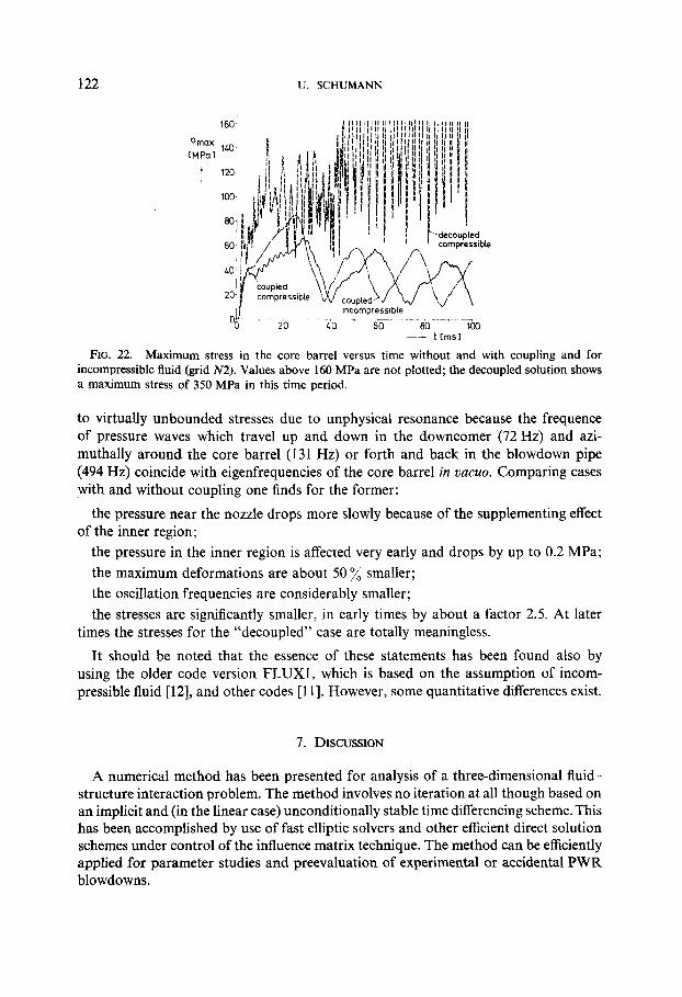
122 U. SCHUMANN

FIG. 22. Maximum stress in the core barrel versus time without and with coupling and for incompressible fluid (grid N2). Values above 160 MPa are not plotted; the decoupled solution shows a maximum stress of 350 MPa in this time period.

to virtually unbounded stresses due to unphysical resonance because the frequence of pressure waves which travel up and down in the downcomer (72 Hz) and azimuthally around the core barrel (131 Hz) or forth and back in the blowdown pipe (494 Hz) coincide with eigenfrequencies of the core barrel in uacuo. Comparing cases with and without coupling one finds for the former:

the pressure near the nozzle drops more slowly because of the supplementing effect of the inner region;

the pressure in the inner region is affected very early and drops by up to 0.2 MPa; the maximum deformations are about 50 % smaller; the oscillation frequencies are considerably smaller; the stresses are significantly smaller, in early times by about a factor 2.5. At later

times the stresses for the “decoupled” case are totally meaningless.

It should be noted that the essence of these statements has been found also by using the older code version FLUXl, which is based on the assumption of incompressible fluid [12], and other codes [l I]. However, some quantitative differences exist.

7. DISCUSSION

A numerical method has been presented for analysis of a three-dimensional fluid- structure interaction problem. The method involves no iteration at all though based on an implicit and (in the linear case) unconditionally stable time differencing scheme. This has been accomplished by use of fast elliptic solvers and other efficient direct solution schemes under control of the influence matrix technique. The method can be efficiently applied for parameter studies and preevaluation of experimental or accidental PWR blowdowns.


The physical model is based on the following assumptions: (a) subcooled fluid, (b) potential flow, (c) constant speed of sound, (d) friction forces which are strictly proportional to the local velocity (“bulk friction”) only, (e) small density changes, (f) small structural deflections, (g) linear-elastic structural material behavior. These assumptions have been justified by order of magnitude estimates (see Appendix) and by comparison to the RS16B experiments in [3, 171. Further assessment of their validity is expected from the planned HDR experiment.

From the experiences gained up to now (see also [3]), we conclude that the largest uncertainties stem from the crude friction model and the pipe break model. The assumption of constant speed of sound seems to be well acceptable for the subcooled regime. In fact, even with an incompressible* fluid (a = co) the resultant deformations differ only by about 10% [12]. This can be understood, e.g., by the fact that the effective speed of sound as given in Eq. (46) is mainly determined by the compressibility of the structure and not so much by that of the fluid. If a is increased from 1088 mjsec to infinity, a’ changes only 17 % in the case of the HDR. In fact, as can be seen from Fig. 22, in the incompressible case the maximum stresses are larger by only about 30 I;;;.

The code FLUX2 is a typical example of a special purpose code. Only by making use of many of the specific properties of the problem was it possible to achieve the efficiency. Despite the rapid enhancement in computer power during the past decade such an approach appears to be preferable in many cases for the solution of large multidimensional time-dependent problems over the use of general purpose codes which often absorb an excessive amount of computer time.

The method is based on linear-elastic structural models, a linear equation of state for the fluid, and the assumption of small wall deflections. All these assumptions together allow for linearization of the coupled fluid pressure and structural deformation equations which in turn enables one to construct an unconditionally stable solution scheme. This property is attractive even in cases where one does not want to apply direct solvers. The assumptions cited might be well acceptable in many other fluid-structure interaction problems.

APPENDIX: DISCUSSION OF MODEL ASSUMPTIONS

Order of magnitude estimates are given here to justify the main physical model assumptions listed in Section 7.

If dp - pu - p, is the difference between initial pressure and saturation pressure, then the mean pressure drops to the saturation pressure according to the outflow velocity, which is of order urnax = (2dp/~)l’~, the break area nRs2, the vessel volume V, and the fluid compressibility measured in terms of the speed of sound a and fluid density p0 in a time of the order

7ma.x = I’ dp/(nR,2a2poumax). (Al)

* With ~1 mm p. prescribed at the upper vessel lid as indicated in Fig. 3.

124 U. SCHUMANN

For the case of the HDR, 7msx = 113 msec. This time is larger than the characteristic oscillation time of the structure. For the beam mode, the oscillation period can be estimated [3] as

7, = ~‘L,2[p,/(5EH~HR)]l~2, (4

which is 93 msec for the HDR. The maximum stress appears in this period (see Fig. 16). Thus a model assuming subcooled fluid is appropriate for this time.

With respect to the assumption of potential flow, it is helpful to estimate the time 7t during which vorticity is built up. As the Reynolds number u~~~R,~~,/~ = 9.3 x IO’, which is relevant for the blowdown pipe with radius R,? , indicates turbulent flow, the time estimate has to include an effective turbulent viscosity qt:

Taking Prandtl’s mixing-length model [32], +qt = pJ2 1 2ujar ~ * p,,(O. 1 Rs)z~max/Rs , one obtains

it = 1 OOR.&max , @3)

=83 msec for the HDR. Thus friction becomes important in the blowdown-pipe relatively early. For this reason a crude friction model is included which is roughly suited for a one-dimensional pipe model. In the downcomer, the velocities are much smaller so that a potential flow model is sufficient in this respect. Departure from potential flow is caused also by density variations which are of the order

dplp” = op/(a2p,) = #hax/u)’ (A41

=0.006 for the HDR. But this value is small for the subcooled period. The structural deflections (see Fig. 14) have been found to be of the order of I “/;;

of the downcomer width HR , which justifies the linearized coupling model. Even more, the deflections are small in comparison to the shell radius RM , and the maximum computed stresses are below the yield-strength (a 150 MPa) so that a linear-elastic structural model is appropriate for the core barrel.

The speed of sound for subcooled water, for 5 MPa < p < 11 MPa, and for temperatures above 200°C varies between 806 and 1360 m/set. The effect of these variations are small as discussed in Section 7.

The main conclusions do not change if the parameter values are taken from a typical PWR instead of from the HDR.

NOMENCLATURE

1. General Notation

a any scalar Qi , aij , aijk components of a vector a a three-dimensional vector


2. Indices

= {a#),, a multidimensional vector components of a matrix

A = [Ai,j]p a matrix ci time derivative diag(atiJ) diagonal matrix with elements ati)

I’ = Radial, j = axial, k = 0, I,..., N azimuthal, m = I, 2 ,..., M axial structural form-function, n (lower) = 0, f,..., N cosine mode (azimuthally), n (upper) = 0, 1 ,..., llmax time index. 0 = initial, 1 = boundary value, max = maximum value, D to the nozzle, S to the blowdown-pipe, w to the core barrel wall.

3. Frequently Used Variables

a 4

L I It4 u N P r t U

V

W

X

X

it= 4.

break

K

A(i)

A2

A

P u

;

* w

speed of sound principal structural coordinates generalized structural coordinates (modes) = $+,u2, kinetic energy per unit fluid volume unit matrix number of axial form functions inner normal of the fluid boundary maximum azimuthal or modal index pressure radial coordinate time velocity vector form-function ansatz structural deflection vector space position eigenvector matrix axial coordinate (downward) Newmark parameter break time fluid bulk damping coefficient eigenvalue of the structural equations Helmholtz parameter diagonal eigenvalue matrix density stress azimuthal coordinate velocity potential = 6 + K@, auxihry potential

angular eigenfrequency

126 U. SCHUMANN

ACKNOWLEDGMENTS

The author is grateful to Dr. A. Ludwig who provided the CYLDYZ subroutines, to Mr. W. Olbrich for his assistance in preparing the computer plots, and to Dr. E. G. Schlechtendahl for many stimulating discussions.

REFERENCES

1. U. SCHUMANN (Ed.), “Computers, Fast Elliptic Solvers and Applications,” Proceedings of the GAMM-Workshop on Fast Solution Methods for the Discretized Poisson Equation, Karlsruhe, March 3-4, 1911, Advance Pub]., London, 1978.

2. B. L. BUZBEE, F. W. DORR, J. A. GEORGE, AND G. H. GOLLJB, SIAM J. Numer. Anal. 8 (1971), 722.

3. U. SCHUMANN, “Effektive Berechnung dreidimensionaler Fluid-Struktur-Wechselwirkung beim Kiihlmittelverluststijrfall eines Druckwasserreaktors-FLUX,” Habilitation thesis, Univ. Karsruhe, Kernforschungzentrum Karlsruhe, KfK 2645, 1978.

4. A. LUDWIG AND R. KRIEG, Nucl. Eng. Des. 43 (1977), 431. 5. R. KRIEG, E. G. SCHLECHTENDAHL, AND K.-H. SCHOLL, Nucl. Eng. Des. 43 (1977), 419. 6. R. L. CLOUD, Nucl. Eng. Des. 46 (1978), 273. 7. T. GRILLENBERGER AND B. OESTERLE, “A Novel Technique for Calculating Fluid Dynamic Pheno-

mena with Respect to Structural Feedback,” 4th Int. Conf. on Struct. Mech. in Reactor Techn., paper B2/5, San Francisco, August 15-19, 1977.

8. J. K. DIENES, C. W. HIRT, AND L. R. STEIN, in “Computational Methods for Fluid-Structure Interaction Problems” (T. Belytschko and T. L. Geers, Eds.), p. 15, ASME, New York, 1977. See also Los Alamos Sci. Lab., LA-NUREG-6772-MS (1977).

9. F. KATZ AND E. G. SCHLECHTENDAHL, “Coupled Fluid-Structure Analysis of the Core Barrel Behavior during Blowdown,” 5th Int. Conf. on Struct. Mech. in Reactor Techn., paper B6/6, Berlin, August 13-17, 1979.

IO. R. KRIEG, E. G. SCHLECHTENDAHL, K.-H. SCHOLL, AND U. SCHUMANN, “Full-Scale HDR Blowdown Experiments as a Tool for Investigating Dynamic Fluid-Structural Coupling,” 4th Int. Conf. on Struct. Mech. in Reactor Techn., paper BSjl, San Francisco, August 15-19, 1977.

11. E. G. SCHLECHTENDAHL, Nucl. Saf?fy 20 (1979), 551. 12. U. SCHUMANN, ilz “Recent Developments in Theoretical and Experimental Fluid Mechanics”

(U. Miiller et al., Eds.), p. 577, Springer-Verlag, Berlin, 1979. 13. W. C. RIVARD AND M. D. TORREY, “Fluid-Structure Response of a Pressurized Water Reactor

Core Barrel during Blowdown," Los Alamos Sci. Lab. LA-7404, 1978. 14. U. SCHUMANN, G. ENDERLE, F. KATZ, A. LUDWIG, H. M~SINGER, AND E. G. SCHLECHTENDAHL,

“Fluid-Structure-Interactions in PWR Vessels during Blowdown-Code Development at Karls- ruhe and Results,” 5th Tnt. Conf. on Struct. Mech. in Reactor Techn., paper B6/1, Berlin, August 13-17, 1979.

15. U. SCHUMANN, “Fluid-Structure Interactions in One-Dimensional Linear Cases,” Kern- forschungzentrum Karlsruhe, KfK 27238, 1979.

16. Battelle-Institut, “Ergebnisse der ersten DWR-Versuche mit Einbauten (DWRI-DWRS),” Frankfurt, report BF-RS 00168-10-1, 1977.

17. U. SCHUMANN, “Analysis of the RS16B Experiment on Fluid-Structure Interactions during PWR-Blowdown,” 5th Int. Conf. on Struct. Mech. in Reactor Techn., paper B6/4. Berlin, August 13-17, 1979.

18. R. E. D. BISHOP, G. M. L. GLADWELL, AND S. MICHAELSON, “The Matrix Analysis of Vibration,” Cambridge Univ. Press, London/New York, 1965.

19. F. C. NELSON AND R. GREIF, Nucl. Eng. Des. 31 (1976), 65. 20. N. M. NEWMARK, J. Eng. Dk,. ASCE 85 (1959) No. EM3, 67.


21. U. SCHUMANN, “Transient Potential Flow in Complex Geometry with Applications to PWR- Blowdown Flows,” Kernforschungszentrum Karlsruhe KFK 2324, 1976, Engl. transl. in EURFNR-1408.

22. .I. W. Coot~r, P. A. W. LEWIS, AND P. D. WELCH, J. Sound Vibr. 12 (1970), 3 15. 23. U. SCHUMANN AND R. A. SWEET, J. Comput. Phys. 20 (1976), 171. 24. U. SCHUMANN AND R. A. SWEET, in “Proceedings, 5th international Conference on Numerical

Methods in Fluid Dynamics,” Lecture Notes in Physics, No. 59, p. 398, Springer-Verlag, Berlin, 1976.

25. B. L. BUZBEE, G. H. GOLUB, AND C. W. NIELSON, S/AM J. Numer. Anal. 7 (1970), 627. 26. B. L. BUZBEE, “Application of Fast Poisson Solvers to the Numerical Approximation of Parabolic

Problems,” thesis, Los Alamos, LA-4950-T, 1972. 27. U. SCHUMANN, in “Computational Fluid Dynamics” (W. Kollmann, Ed.), Q. 401, Hemisphere,

Washington, New York, London, 1980. 28. U. SCHUMANN, in “Proceedings, 2nd GAMM-Conference on ‘Numerical Methods in Fluid

Mechanics’ ” (E. H. Hirschel and W. Geller, Eds.), p. 192, DFVLR, K6ln, 1977. 29. R. SCHUSTER, Angew. Informat& 3177 (1977), 155. 30. K. LEINEMANN AND E. G. SCHLECHTENDAHL, in “CAD Systems” (J. J. Allan, Ed.), p. 143, North-

Holland, Amsterdam, 1977. 31. D. J. KORTEWEG, Ann. Phys. Chem. 5 (1878), 525. 32. H. SCHLICHTING, “Grenzschicht-Theorie,” p. 539, 560, G. Braun, Karlsruhe, 1965.

Fast Elliptic Solvers and Three-Dimensional Fluid-Structure

Documents

Transcript of Fast Elliptic Solvers and Three-Dimensional Fluid-Structure