Fast Demand Control in Smart Grid Communications with User-in ...
99
Fast Demand Control in Smart Grid Communications with User-in-the-Loop (UIL) Method by Inan Korkmaz A thesis submitted to the Faculty of Graduate and Postdoctoral Affairs in partial fulfillment of the requirements for the degree of Master of Applied Science in Electrical and Computer Engineering Ottawa-Carleton Institute for Electrical and Computer Engineering Department of Systems and Computer Engineering Carleton University Ottawa, Ontario May, 2015 c Copyright Inan Korkmaz, 2015
Transcript of Fast Demand Control in Smart Grid Communications with User-in ...
Fast Demand Control in Smart GridCommunications with User-in-the-Loop (UIL)
Method
by
Inan Korkmaz
A thesis submitted to the
Faculty of Graduate and Postdoctoral Affairs
in partial fulfillment of the requirements for the degree of
Master of Applied Science in Electrical and Computer Engineering
Ottawa-Carleton Institute for Electrical and Computer Engineering
Department of Systems and Computer Engineering
Carleton University
Ottawa, Ontario
May, 2015
c©Copyright
Inan Korkmaz, 2015

The undersigned hereby recommends to the
Faculty of Graduate and Postdoctoral Affairs
acceptance of the thesis
Fast Demand Control in Smart Grid Communications withUser-in-the-Loop (UIL) Method
submitted by Inan Korkmaz
in partial fulfillment of the requirements for the degree of
Master of Applied Science in Electrical and Computer Engineering
Professor Halim Yanikomeroglu, Thesis Supervisor
Professor Roshdy Hafez, Chair, Department of Systems and Computer Engineering
Ottawa-Carleton Institute for Electrical and Computer Engineering
Department of Systems and Computer Engineering
Carleton University
May, 2015
ii

Abstract
Recently, household energy consumption has been highly increasing, although there
is a decrease in the source of energy. Consequently, the base price of electricity has
been rising. Thus, there are a variety of approaches to save electricity costs.
One proposed approach is the User-in-the Loop (UIL) method, in which the con-
sumers (i.e. users) are given satisfactory incentives (for instance decreasing the base
price of the electricity) to postpone their demand until low peak hours. To explore the
effectiveness of this method, this study enrolls the open-loop control model and the
closed-loop control model. While the open-loop control model is related to consumers’
decisions of the process time relying on the low electricity cost, the closed-loop control
model refers to consumer’s reactions to the system’s output and given incentives by
electricity suppliers. To investigate the effectiveness of UIL, both control models are
examined under three types of pricing models; namely, the fixed, current, and the dy-
namic pricing models. Whereas the base price of the electricity is steady in the fixed
pricing model, under the current pricing model, it varies according to specified time
periods in the current pricing model. Additionally, we propose the dynamic pricing
model, in which the base price of the electricity is updated every 5 minutes based on a
feedback message received from users. This feedback message is transmitted through
ZegBee communication collecting the total amount of the electricity consumption of
all home appliances.
As a result of this study, we found that there is an inverse relationship between
the number of users and the efficiency of UIL with the dynamic pricing model.
iii

Acknowledgments
First and foremost, I am most grateful to Allah (God), the Creator and Sustainer
of the Universe, for giving me the ability to complete this work. I wish to extend
my special thanks to my supervisor, Dr. Halim Yanikomeroglu, for his support
and guidance towards achieving the completion of this thesis. I would like to
thank Dr. Rainer Schoenen, Postdoctoral fellow in our group, for his invaluable
help and suggestions throughout my research. Thanks to Ibrahim Aydin, for the
feedback towards improving my work. Thanks to the departmental staff for their
administrative and technical support. I would like to thank all of my friends with
whom I studied; we encouraged one another throughout the course of our studies.
I am deeply grateful to my parents for raising me and for teaching me the most
important things in life. A huge thanks to my wife for her moral support and for
always keeping me cheered up.
iv

List of Abbreviations
5G: 5th Generation
AC: Air Conditioner
ac: Alternative Current
AMI: Advanced Metering Infrastructure
AMR: Automatic Metering Reading
BW: Bandwidth
CDF: Cumulative Distribution Function
CLC: Closed-Loop Control
EU: End User
EUP: End User Price
FDC: Fast Demand Control
IESO: Independent Electricity System Operator
IoE: Internet of Everything
IoTs: Internet of Things
IPv4: Internet Protocol version 4
IPv6: Internet Protocol version 6
M2M: Machine to Machine Communication
NANs: Neighborhood Area Networks
OEB: Ontario Energy Board
OFDM: Orthogonal Frequency Division Multiplexing
OLC: Open-Loop Control
PDF: Power Spectral Density
PID: Proportion Integral Differential
PLC: Power Line Communication
RF: Radio Frequency
RPP: Regulated Price Plan
SG: Smart Grid
SM: Smart Meter
UIL: User-in-the-Loop
UIOL: User-in-the-Open-Loop
v

Table of Contents
Abstract iii
Acknowledgments iv
Table of Contents vi
List of Tables ix
List of Figures x
1 Introduction 1
1.1 5G definition and Internet of Things (IoTs) . . . . . . . . . . . . . . 1
1.2 Fast Demand Control (FDC) in Energy Grid . . . . . . . . . . . . . . 4
1.3 Smart Grid Communications Aspects . . . . . . . . . . . . . . . . . . 5
1.3.1 Smart Meter Structure . . . . . . . . . . . . . . . . . . . . . . 8
1.3.2 Power Line Communications (PLCs) . . . . . . . . . . . . . . 14
1.4 UIL Definition and its Properties . . . . . . . . . . . . . . . . . . . . 16
1.5 ZigBee Communications . . . . . . . . . . . . . . . . . . . . . . . . . 17
1.5.1 802.15.4 ZigBee Physical Layer . . . . . . . . . . . . . . . . . 17
1.5.2 The ZigBee Protocol . . . . . . . . . . . . . . . . . . . . . . . 18
1.5.3 Why Do We Need ZigBee Communications? . . . . . . . . . . 18
1.5.4 Mesh Networks . . . . . . . . . . . . . . . . . . . . . . . . . . 19
1.5.5 The Concept of Open-Loop Control (OLC) and Closed-Loop
Control (CLC) . . . . . . . . . . . . . . . . . . . . . . . . . . 22
1.5.6 Problem Statement . . . . . . . . . . . . . . . . . . . . . . . . 26
1.5.7 Contributions . . . . . . . . . . . . . . . . . . . . . . . . . . . 28
1.5.8 Thesis Organization . . . . . . . . . . . . . . . . . . . . . . . 28
vi

2 System Definition 29
2.1 Pricing Systems Comparisons . . . . . . . . . . . . . . . . . . . . . . 29
2.1.1 Fixed Pricing Model . . . . . . . . . . . . . . . . . . . . . . . 29
2.1.2 Current Pricing Model (Partly Dynamic) . . . . . . . . . . . . 30
2.1.3 Dynamic Pricing Model . . . . . . . . . . . . . . . . . . . . . 31
2.2 Simulation Tools . . . . . . . . . . . . . . . . . . . . . . . . . . . . . 35
2.3 System Model . . . . . . . . . . . . . . . . . . . . . . . . . . . . . . . 37
2.4 Independent Electricity System Operator (IESO) . . . . . . . . . . . 45
2.5 Summary of This Chapter . . . . . . . . . . . . . . . . . . . . . . . . 47
3 Open-Loop Control Model 48
3.1 Fixed Pricing Model . . . . . . . . . . . . . . . . . . . . . . . . . . . 50
3.1.1 One-User One-Appliance Model . . . . . . . . . . . . . . . . . 50
3.1.2 One-User Multi-Appliance Model . . . . . . . . . . . . . . . . 51
3.1.3 Multi-User Multi-Appliance Model . . . . . . . . . . . . . . . 52
3.2 Current Pricing Model . . . . . . . . . . . . . . . . . . . . . . . . . . 53
3.3 Dynamic Pricing Model . . . . . . . . . . . . . . . . . . . . . . . . . 61
3.3.1 One-User One-Appliance Model . . . . . . . . . . . . . . . . . 61
3.3.2 One-User Multi-Appliance Model . . . . . . . . . . . . . . . . 62
3.3.3 Multi-User Multi-Appliance Model . . . . . . . . . . . . . . . 63
3.4 Summary of This Chapter . . . . . . . . . . . . . . . . . . . . . . . . 63
4 Closed-Loop Control Model 65
4.1 Fixed Pricing Model . . . . . . . . . . . . . . . . . . . . . . . . . . . 70
4.2 Current Model . . . . . . . . . . . . . . . . . . . . . . . . . . . . . . 71
4.3 Dynamic Pricing Model . . . . . . . . . . . . . . . . . . . . . . . . . 72
4.4 Summary of This Chapter . . . . . . . . . . . . . . . . . . . . . . . . 72
5 Conclusion and Future Works 74
5.1 Open-Loop Results . . . . . . . . . . . . . . . . . . . . . . . . . . . . 74
5.2 Closed-Loop Results . . . . . . . . . . . . . . . . . . . . . . . . . . . 76
5.3 Conclusion . . . . . . . . . . . . . . . . . . . . . . . . . . . . . . . . . 79
5.3.1 Improvements Over the Current Pricing Model and Future Works 81
List of References 83
vii

Appendix A Equations 87
viii

List of Tables
2.1 Improvements in Dynamic, Current,and Fixed Pricing Models (Cent) 46
5.1 Model Pricing Comparisons . . . . . . . . . . . . . . . . . . . . . . . 79
ix

List of Figures
1.1 Internet of Things (IoTs) Structure [1]. . . . . . . . . . . . . . . . . . 2
1.2 Smart Grid Communication Infrastructures . . . . . . . . . . . . . . . 7
1.3 A Smart Meter (SM) Structure . . . . . . . . . . . . . . . . . . . . . 8
1.4 The Diagram of AMI [2]. . . . . . . . . . . . . . . . . . . . . . . . . . 9
1.5 Time of Use (TOU) Ontario [3]. . . . . . . . . . . . . . . . . . . . . . 10
1.6 Tiered Pricing (Ontario) [4]. . . . . . . . . . . . . . . . . . . . . . . . 11
1.7 5-Year Fixed vs. 6-Month RPP [4]. . . . . . . . . . . . . . . . . . . . 12
1.8 Constant vs. Fluctuating Rates [4]. . . . . . . . . . . . . . . . . . . . 12
1.9 A Typical PLC Model [5]. . . . . . . . . . . . . . . . . . . . . . . . . 15
1.10 User-in-the-Loop (UIL) Model [6]. . . . . . . . . . . . . . . . . . . . . 16
1.11 Mesh Networks . . . . . . . . . . . . . . . . . . . . . . . . . . . . . . 19
1.12 ZigBee Network [7] . . . . . . . . . . . . . . . . . . . . . . . . . . . . 19
1.13 Bluetooth vs. Wi-Fi vs. ZigBee vs. Others [8] . . . . . . . . . . . . . 21
1.14 Open-Loop Model . . . . . . . . . . . . . . . . . . . . . . . . . . . . . 23
1.15 Closed-Loop Control Model . . . . . . . . . . . . . . . . . . . . . . . 24
2.1 Demand and Supply . . . . . . . . . . . . . . . . . . . . . . . . . . . 30
2.2 Supply-Demand-Price Relation [9] . . . . . . . . . . . . . . . . . . . . 31
2.3 On-Off-Peak Hours for Ontario [10] . . . . . . . . . . . . . . . . . . . 32
2.4 Dynamic Pricing for 5 Minutes Cycle . . . . . . . . . . . . . . . . . . 33
2.5 Green-Yellow-Red Regions for Illinois . . . . . . . . . . . . . . . . . . 34
2.6 Green-Yellow-Red Regions for Ontario . . . . . . . . . . . . . . . . . 34
2.7 Sub-Poisson, Poisson, Super Poisson [11]. . . . . . . . . . . . . . . . . 35
2.8 Air Conditioner . . . . . . . . . . . . . . . . . . . . . . . . . . . . . . 36
2.9 System Model . . . . . . . . . . . . . . . . . . . . . . . . . . . . . . . 37
2.10 Price Added to the System from the Utility Company . . . . . . . . . 38
2.11 Backbone of the System Model . . . . . . . . . . . . . . . . . . . . . 38
2.12 Random Selection Among Users . . . . . . . . . . . . . . . . . . . . . 39
x
2.13 Main parameter of the System . . . . . . . . . . . . . . . . . . . . . . 39
2.14 Main Parameter of the Users . . . . . . . . . . . . . . . . . . . . . . . 40
2.15 Counting Days with its Parameters . . . . . . . . . . . . . . . . . . . 40
2.16 General View of Appliances . . . . . . . . . . . . . . . . . . . . . . . 41
2.17 Fridge is an Example of non-Shiftable Demand . . . . . . . . . . . . . 42
2.18 The Recover Parameters for non-Shiftable Demand . . . . . . . . . . 42
2.19 Constant Values for Appliance Models . . . . . . . . . . . . . . . . . 43
2.20 Prices are Calculated Based on the Consumed Energy . . . . . . . . . 43
2.21 Calculating the Total Payment . . . . . . . . . . . . . . . . . . . . . . 44
2.22 Calculating the Total Consumption . . . . . . . . . . . . . . . . . . . 44
2.23 Dynamic, Current, and Fixed Pricing Models . . . . . . . . . . . . . . 46
3.1 Example for Open-Loop Control Model . . . . . . . . . . . . . . . . . 48
3.2 Open-Loop Control Model Road Map . . . . . . . . . . . . . . . . . . 49
3.3 Linear Graph . . . . . . . . . . . . . . . . . . . . . . . . . . . . . . . 51
3.4 Fixed Pricing Model . . . . . . . . . . . . . . . . . . . . . . . . . . . 52
3.5 Current Pricing Rate with Threshold Values . . . . . . . . . . . . . . 54
3.6 PDF, CDF and Histogram of X (Base Price) . . . . . . . . . . . . . . 55
3.7 One-User One-Appliance Model . . . . . . . . . . . . . . . . . . . . . 59
3.8 Multi-User Multi-Appliances Model . . . . . . . . . . . . . . . . . . . 60
3.9 One-User One-Appliance Model . . . . . . . . . . . . . . . . . . . . . 62
3.10 Multi-User Multi-Appliance Model . . . . . . . . . . . . . . . . . . . 64
4.1 Closed-Loop Models . . . . . . . . . . . . . . . . . . . . . . . . . . . 66
4.2 PID Controller . . . . . . . . . . . . . . . . . . . . . . . . . . . . . . 67
4.3 Closed-Loop Control Model . . . . . . . . . . . . . . . . . . . . . . . 68
4.4 Temporal Probability with Postponed Time [12]. . . . . . . . . . . . . 69
4.5 The Outline of Closed-Loop Control Model . . . . . . . . . . . . . . . 70
4.6 Fixed Pricing System for Closed-Loop Model . . . . . . . . . . . . . . 71
4.7 Current Pricing System for Closed-Loop Model . . . . . . . . . . . . 72
4.8 Dynamic Pricing System for Closed-Loop Model . . . . . . . . . . . . 73
5.1 Supply Curve . . . . . . . . . . . . . . . . . . . . . . . . . . . . . . . 75
5.2 Demand Curve . . . . . . . . . . . . . . . . . . . . . . . . . . . . . . 75
5.3 Electricity Price Distribution . . . . . . . . . . . . . . . . . . . . . . . 76
5.4 One-User One-Appliance . . . . . . . . . . . . . . . . . . . . . . . . . 77
5.5 Multi-User Multi-Appliance Model for Open-Loop Control Model . . 78
xi

5.6 Multi-User Multi-Appliance Model for Closed-Loop Control Model . . 79
5.7 Comparison of Simulated Models with Different Number of Users w/o
UIL Method . . . . . . . . . . . . . . . . . . . . . . . . . . . . . . . . 80
xii
Chapter 1
Introduction
1.1 5G definition and Internet of Things (IoTs)
The main idea in a cellular network is to meet the required demand in data rate,
coverage, speed, etc. 5G (5th generation mobile networks) promises to its users high
data rates of several tens of Mb/s supported for hundreds of users and 1 Gb/s si-
multaneously to tens of workers on the same office floor. Likewise, 5G allows up to
several 100,000s of simultaneous connections to support massive sensor deployments.
Furthermore, it improves coverage and enhances signal efficiency. This technology
will be rolled out by 2020 to meet business and consumer demands. Without going
into more detail, it is important to mention another aspect of 5G in regards to its
application. 5G should not be considered only for layers 1, 2, or 3. Moreover, 5G
comes with its applications which are called Internet of Things (IoT), or Internet of
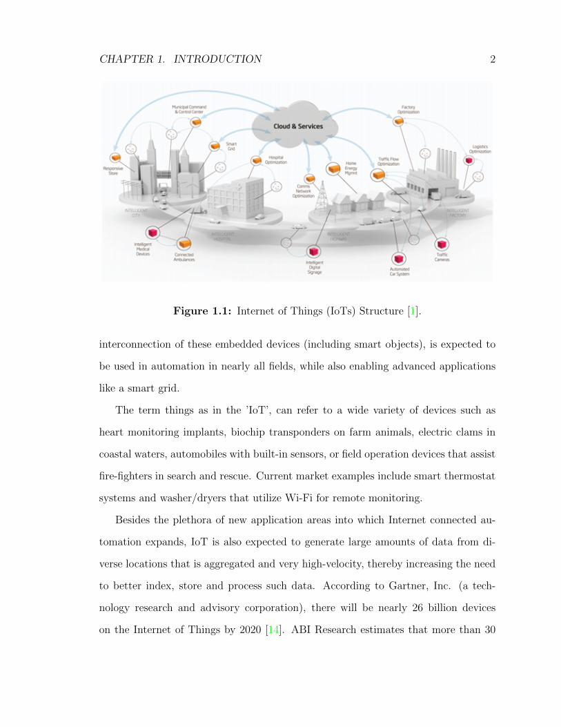
Everything (IoE), as recently introduced in literature, see Figure 1.1. The IoT is the
interconnection of uniquely identifiable embedded computing devices within the exist-
ing Internet infrastructure. Typically, IoT is expected to offer advanced connectivity
of devices, systems, and services that goes beyond machine-to-machine communica-
tions (M2M) and covers a variety of protocols, domains, and applications [13]. The
1
CHAPTER 1. INTRODUCTION 2
Figure 1.1: Internet of Things (IoTs) Structure [1].
interconnection of these embedded devices (including smart objects), is expected to
be used in automation in nearly all fields, while also enabling advanced applications
like a smart grid.
The term things as in the ’IoT’, can refer to a wide variety of devices such as
heart monitoring implants, biochip transponders on farm animals, electric clams in
coastal waters, automobiles with built-in sensors, or field operation devices that assist
fire-fighters in search and rescue. Current market examples include smart thermostat
systems and washer/dryers that utilize Wi-Fi for remote monitoring.
Besides the plethora of new application areas into which Internet connected au-
tomation expands, IoT is also expected to generate large amounts of data from di-
verse locations that is aggregated and very high-velocity, thereby increasing the need
to better index, store and process such data. According to Gartner, Inc. (a tech-
nology research and advisory corporation), there will be nearly 26 billion devices
on the Internet of Things by 2020 [14]. ABI Research estimates that more than 30

CHAPTER 1. INTRODUCTION 3
billion devices will be wirelessly connected to the Internet of Things (Internet of Ev-
ery Things) by 2020 [15]. As per a recent survey and study done by Pew Research
Internet Project, a large majority of the technology experts and engaged Internet
users who responded 83% agreed with the notion that the Internet/cloud of things,
embedded and wearable computing (and the corresponding dynamic systems) will be
widespread and have beneficial effects by 2025. It is clear that the IoT will consist of
a large number of devices being connected to the Internet.
Integration with the Internet implies that devices will utilize an IP address as a
unique identifier. However, due to the limited address space of IPv4 (which allows for
4.3 billion unique addresses), objects in the IoT will have to use IPv6 to accommodate
the significant address space required [16]. Objects in the IoT will not only be devices
with sensory capabilities, but they will also provide actuation capabilities (e.g., bulbs
or locks controlled over the Internet).
To a large extent, the future of the IoT will not be possible without the support
of IPv6; and consequently the global adoption of IPv6 in the coming years will be
critical for the successful development of the IoT in the future.
IoTs has ability to network embedded devices with limited CPU, memory, and
power resources demonstrates that it can find applications in nearly every field. Such
systems could be in charge of collecting information in settings ranging from natural
ecosystems to buildings and factories, thereby finding applications in the environmen-
tal sensing and urban planning fields.
On the other hand, IoT systems could also be responsible for performing actions,
not just sensing things. Intelligent shopping systems, for example, could monitor
specific users’ purchasing habits in a store by tracking their mobile phones. With
the IoT producers can provide users with special offers on their favourite products
and locate items of interest which their refrigerator automatically conveys to the

CHAPTER 1. INTRODUCTION 4
phone. Additional examples of sensing and actuating are reflected in applications
that deal with heat, electricity and energy management, as well as cruise-assisting
transportation systems.
1.2 Fast Demand Control (FDC) in Energy Grid
After some introduction in the IoT, now it is time to make a definition of Fast De-
mand Control (FDC). FDC refers to the rapid demand cutbacks that can be achieved
”within the flick of a switch”, for instance, from turning point of a home appliance,
such as an air conditioner, dryer or lights. FDC is the key factor for users (ustomers),
for controlling their energy usage instantly called dynamic control of energy usage.
Since users are able to use their energy instantly, they are also able to manage the
usage time. Before turning on their appliances (dryer, washer, air conditioner, etc.)
users are supposed to check the cost of electricity on the screen of smart appliances
or cell phones. After seeing the information on the screen, they make a decision
based on the lower electricity price range. Users will see the prices instantly from
low to high through different indicators (numerical information, coloured indicator,
warning beep, a scale, etc.). These indicators give information about the electricity
price in each 5 minute cycle. In my model, I use the three universal colour indicators:
green colour are used for lower electricity prices. When users see the green colour
on the smart device’s screen, they understand that it is a suitable time to turn on
their appliances. The green colour is chosen based on τ1 value, which is the upper
boundary of green colour. Users are supposed to use their appliances or electric cars
with the probability of (PON = 1, POFF = 0) to get incentives. When users turn
on their smart appliances or charge electric cars ahead of time, they will get some
incentives which can be bonus points to direct discount in electricity bills. Applying
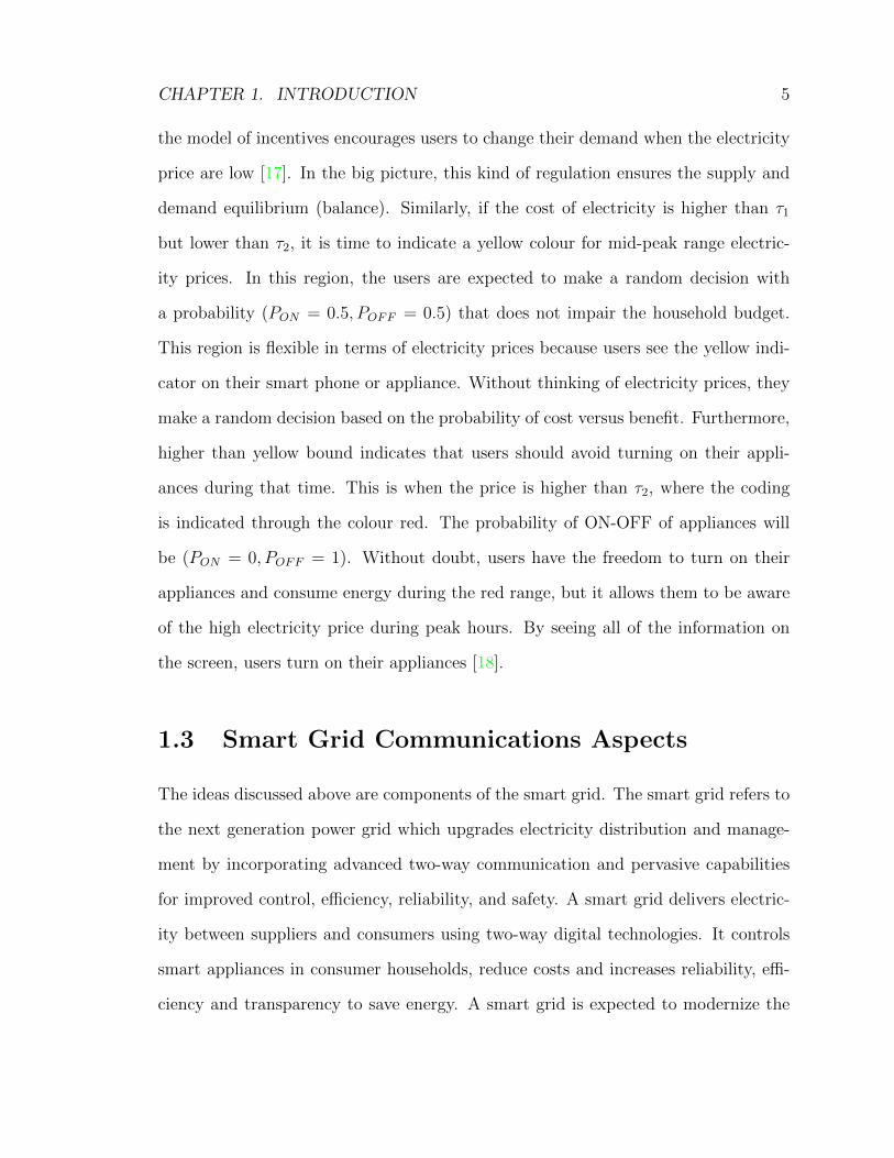
CHAPTER 1. INTRODUCTION 5
the model of incentives encourages users to change their demand when the electricity
price are low [17]. In the big picture, this kind of regulation ensures the supply and
demand equilibrium (balance). Similarly, if the cost of electricity is higher than τ1
but lower than τ2, it is time to indicate a yellow colour for mid-peak range electric-
ity prices. In this region, the users are expected to make a random decision with
a probability (PON = 0.5, POFF = 0.5) that does not impair the household budget.
This region is flexible in terms of electricity prices because users see the yellow indi-
cator on their smart phone or appliance. Without thinking of electricity prices, they
make a random decision based on the probability of cost versus benefit. Furthermore,
higher than yellow bound indicates that users should avoid turning on their appli-
ances during that time. This is when the price is higher than τ2, where the coding
is indicated through the colour red. The probability of ON-OFF of appliances will
be (PON = 0, POFF = 1). Without doubt, users have the freedom to turn on their
appliances and consume energy during the red range, but it allows them to be aware
of the high electricity price during peak hours. By seeing all of the information on
the screen, users turn on their appliances [18].
1.3 Smart Grid Communications Aspects
The ideas discussed above are components of the smart grid. The smart grid refers to
the next generation power grid which upgrades electricity distribution and manage-
ment by incorporating advanced two-way communication and pervasive capabilities
for improved control, efficiency, reliability, and safety. A smart grid delivers electric-
ity between suppliers and consumers using two-way digital technologies. It controls
smart appliances in consumer households, reduce costs and increases reliability, effi-
ciency and transparency to save energy. A smart grid is expected to modernize the
CHAPTER 1. INTRODUCTION 6
legacy electricity network. It provides automatic monitoring, protecting and opti-
mizing to the operation of the interconnected elements. It covers traditional central
generators and/or emerging renewal distributed generators, through a transmission
network and distribution system, and to industrial consumer as well as household con-
sumers with their thermostats, electric vehicles, and smart appliances [19]. A smart
grid is characterized by the bidirectional connection of electricity and information
flows, to create an automated, widely distributed delivery network. It incorporates
the legacy electricity grid, with the benefits of modern communication, to deliver real-
time information and enable the near-instantaneous balance of supply and demand
management. A smart grid is adopted in many technologies that are already in use
in industrial applications, such as a wireless network in telecommunications, sensor
networks in manufacturing, and now is adopted in new intelligent and interconnected
technologies [20]. We can divide the smart grid communications technology into five
groups:
• Integrated communications
• Advanced components
• Sensing and measurements
• Improved interfaces and decision support
• Standards and groups.
Figure 1.2 illustrates a general architecture of smart grid communication infras-
tructures. Smart grids distribute electricity between generators (both traditional
power generation and distributed generation sources) and users (industrial, commer-
cial, residential consumers) using bi-directional information flow to control consumers

CHAPTER 1. INTRODUCTION 7
Figure 1.2: Smart Grid Communication Infrastructures
intelligent appliances. Thus, saving energy consumption and reducing the consequent
expense, meanwhile increasing system reliability and operation transparency. With
a communication infrastructure, the smart metering/monitoring techniques can pro-
vide the real-time energy consumption as feedback and correspond to the demand
to/from utilities. The network operation centre can retrieve the customer power us-
age data and the on-line market pricing from data centres, to optimize the electricity
generation and distribution, according to the energy consumption [21].
The key point of smart grid communications is the ability of different variables
(e.g. intelligent devices, dedicated software, processes, control centre, etc.) to interact
through a communication infrastructure [22].
Current electrical utility Wide Area Networks (WANs) consist of hybrid commu-
nication, such as wired communications (fiber optics), power line communications
(PLC), copperwire line, and various wireless technologies (data communications in
cellular networks such as GSM/GPRS/WiMax/WLAN and Cognitive Radio) [23].
CHAPTER 1. INTRODUCTION 8
Figure 1.3: A Smart Meter (SM) Structure
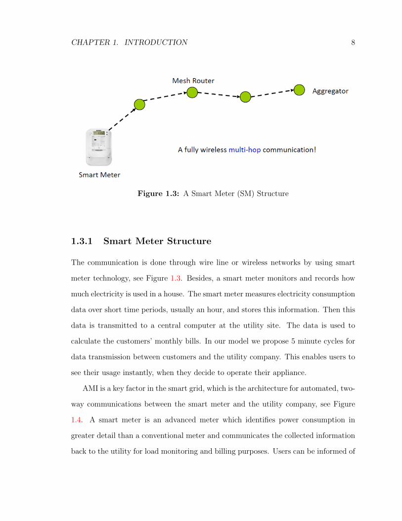
1.3.1 Smart Meter Structure
The communication is done through wire line or wireless networks by using smart
meter technology, see Figure 1.3. Besides, a smart meter monitors and records how
much electricity is used in a house. The smart meter measures electricity consumption
data over short time periods, usually an hour, and stores this information. Then this
data is transmitted to a central computer at the utility site. The data is used to
calculate the customers’ monthly bills. In our model we propose 5 minute cycles for
data transmission between customers and the utility company. This enables users to
see their usage instantly, when they decide to operate their appliance.
AMI is a key factor in the smart grid, which is the architecture for automated, two-
way communications between the smart meter and the utility company, see Figure
1.4. A smart meter is an advanced meter which identifies power consumption in
greater detail than a conventional meter and communicates the collected information
back to the utility for load monitoring and billing purposes. Users can be informed of
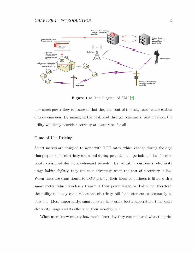
CHAPTER 1. INTRODUCTION 9
Figure 1.4: The Diagram of AMI [2].
how much power they consume so that they can control the usage and reduce carbon
dioxide emission. By managing the peak load through consumers’ participation, the
utility will likely provide electricity at lower rates for all.
Time-of-Use Pricing
Smart meters are designed to work with TOU rates, which change during the day;
charging more for electricity consumed during peak-demand periods and less for elec-
tricity consumed during low-demand periods. By adjusting customers’ electricity
usage habits slightly, they can take advantage when the cost of electricity is low.
When users are transitioned to TOU pricing, their home or business is fitted with a
smart meter, which wirelessly transmits their power usage to HydroOne; therefore,
the utility company can prepare the electricity bill for customers as accurately as
possible. Most importantly, smart meters help users better understand their daily
electricity usage and its effects on their monthly bill.
When users know exactly how much electricity they consume and what the price

CHAPTER 1. INTRODUCTION 10
Figure 1.5: Time of Use (TOU) Ontario [3].
will be at a given time, they get the chance to make a smarter decision for energy us-
age. Users should be able to save money by reducing their electricity usage during the
peak hours, through pricing that rewards them for shifting their heaviest electricity
usage to off-peak hours, see Figure 1.5.
Tiered (Normal Meter) Pricing
There are two different prices on monthly bills and slight changes between winter
and summer seasons because the customers are on a tiered pricing plan (RPP). Two
different prices are set twice a year by the Ontario Energy Board. One price applies
up to a certain threshold and a higher price applies if the users go over this threshold,
see Figure 1.6.

CHAPTER 1. INTRODUCTION 11
Figure 1.6: Tiered Pricing (Ontario) [4].
5-Year Fixed vs. 6-Month RPP Rates
The decision on whether to lock in users’ RPP rates depends on their risk tolerance
and the degree to which they feel rates are likely to increase in the future.
As can be seen from Figure 1.7, the following hydro rate chart is a sample. When
the users lock in their hydro rate, they tend to pay their contract, but in the later
years of their contract they tend to pay less than the variable rate.
Another factor to be considered is when users use most of their electricity. The
highest (on peak) rate of 14 cents/kWh is from 7:00 AM to 11:00 AM and from 5:00
PM to 7:00 PM in winter. In the summer, the on peak rate is from 11:00 AM to 5:00
PM weekdays. If households are busy during these times, and they stay with the
RPP, they will be using a lot of power at the peak rates. By switching to a fixed-rate
plan, they are not penalized when using power during peak-demand periods. The
chart below shows how your Smart Meter allows your utility to be charged a different
rate at different times of the day, see Figure 1.8.

CHAPTER 1. INTRODUCTION 12
Figure 1.7: 5-Year Fixed vs. 6-Month RPP [4].
Figure 1.8: Constant vs. Fluctuating Rates [4].

CHAPTER 1. INTRODUCTION 13
With smart meters and time-of-use rates, distribution companies can provide de-
tailed information on the customer web portal, MyHydroLink, itemizing how much
electricity was consumed and when it was consumed. The bill also displays the three
rate periods and the amount of consumption used within those periods. This is in-
tended to encourage customers to shift ther consumption, where it is possible, to
lower-cost times of the day and week, and to more actively manage their electricity
usage. The benefit of using a smart meter is that when Ontario electricity consumers
shift their usage to off-peak hours, it reduces peak demand on the provincial elec-
tricity system. Over the longer term, lower peak demand will mean a reduced need
for new generating, transmission and distribution infrastructure, lowering costs for
all Ontarians. In addition, a reduction in peak demands means that the province
can also reduce its use of carbon dioxide emitting generators that are called on when
demand is high, lowering greenhouse gas emissions. Smart meter data also provides
comprehensive, detailed information for electricity system planning, allowing plan-
ners to identify where future generation, transmission and distribution investments
are required. Smart meters also help LDCs identify power theft and respond to meter
failures and outages more quickly, and they help LDCs identify greater operational
efficiencies in local distribution system management. This efficiency lowers the elec-
tricity costs for customers. The infrastructure of a smart grid is similar to a telephone
or Internet connection.
In our model, we use a dynamic pricing model based on the real and instant data
from the HydroOttawa web page. This method is more reliable than the three rate
period, because the model that is still in use in Ottawa is partly dynamic, rather
than fully dynamic. Users are encouraged to use their power in a low-cost time, but
this can lead to high consumption of energy in the low-cost time period. However,
with dynamic pricing, user will see instant changes in price. This method increases

CHAPTER 1. INTRODUCTION 14
the awareness of saving money and energy.
1.3.2 Power Line Communications (PLCs)
PLC uses the power feeder line as communication media in Figure 1.9. The first gen-
eration ripple control systems provide one-way communications, in which centralized
load control and peak shaping have been performed for many years. The European
standards body CENELEC restricted the use of frequencies between 3 kHz and 95
kHz for two-way communications for electricity distributor use. A number of second
generation PLC systems with low data rates were proposed in the 1990s, and AMR
systems have been deployed based on this technology. Third generation systems based
on OFDM with much higher data rates are currently being developed and deployed for
smart grids, distribution automation and advanced metering management [24]. When
the smart grid was developed, the importance of PLC and distribution networks be-
came an important technology for transmitting the information between users and
utility companies. To provide service between users and utility companies, the PLC
design has to be improved with reliable data rates. Understanding PLC parameters
are vital for two-way communication for the sake of high data rates and efficiency
of the system. The main thing influencing the reliable communication of high-speed
data on power lines is the attenuation of the high-frequency signal, which exhibits
more obviously in the branch of power lines. It is almost impossible to use the fre-
quency range of 10 to 20 MHz for the reliable communications from the distributing
transformer to the user, so it must be solved with the aid of repeaters and modulation
schemes.

CHAPTER 1. INTRODUCTION 15
Figure 1.9: A Typical PLC Model [5].

CHAPTER 1. INTRODUCTION 16
Figure 1.10: User-in-the-Loop (UIL) Model [6].
1.4 UIL Definition and its Properties
The idea of User in the Loop (UIL) is pointed out for users’ ”wireless behaviour” and
aimed to control their behaviours to increase the efficiency of wireless data resources
without limiting bandwidth (BW) [25]. Dr. Rainer Schoenen explores this idea in his
paper, where he proposed that balancing or almost balancing the demand and supply
will increase the efficiency of using wireless resources. In his paper [26], he focuses on
controlling the demand side control; he pointed out that the control model is divided
into two parts: Spatial control that users are encouraged to change their location to
get higher data and avoid data traffic congestion [27], [28]. In temporal control, users
are supposed to postpone their current data demand in case of congestion [29]. When
users take any of these control models to avoid congestion, they are incentivized from
the reduction on their monthly bill, bonus points, increase in the speed of data. etc.
Incentives are based on instant data (i.e. they are dynamic) to ensure that the user
reduces his or her usage. In Dr. Schoenen’s public survey on how people react by
changing their location or postponing the usage of their data, Dr. Schoenen indicates
that people react positively towards these two control models, see Figure 1.10.

CHAPTER 1. INTRODUCTION 17
1.5 ZigBee Communications
1.5.1 802.15.4 ZigBee Physical Layer
ZigBee communications is open to global wireless standards to provide the foundation
for the Internet of Things by enabling simple and smart objects to work together, im-
proving comfort and efficiency in everyday life. ZigBee is developed as an open global
standard to address the unique needs of low-cost, low-power wireless M2M networks.
The ZigBee standard operates on the IEEE 802.15.4 physical radio specification and
operates in unlicensed bands including 2.4 GHz, 900 MHz and 868 MHz 1.
IEEE 802.15.4 specification
• 802: networking group
• 15: wireless network
• 4: low data rate consuming less power
The 802.15.4 specification upon which the ZigBee stack operates gained ratifica-
tion by the Institute of Electrical and Electronics Engineers (IEEE) in 2003. The
specification is a packet-based radio protocol intended for low-cost, battery-operated
devices. The protocol allows devices to communicate in a variety of network topolo-
gies and can have battery life lasting several years.
802.15.4 Basics:
• 868.0-868.6 MHz: Europe, allows one communication channel.
• 902-928 MHz: North America, up to ten channels (2003), extended to thirty
(2006).
1In stead of ZegBee, Wi-fi can be used.

CHAPTER 1. INTRODUCTION 18
• 2400-2483.5 MHz: Worldwide use, up to sixteen channels (2003, 2006).
1.5.2 The ZigBee Protocol
Member of the ZigBee alliance have created and ratified the ZigBee protocol. Over 300
leading semiconductor manufacturers, technology firms, OEMs and service companies
comprise the ZigBee Alliance membership. The ZigBee protocol was designed to
provide an easy-to-use wireless data solution characterized by secure, reliable wireless
network architectures.
1.5.3 Why Do We Need ZigBee Communications?
The ZigBee protocol is designed to communicate data through hostile RF environ-
ments that are common in commercial and industrial applications, see Figure 1.12.
ZigBee protocol features include:
• Support for multiple network topologies such as point-to-point, point-to-multi
point and mesh networks.
• Low duty cycle provides long battery life
• Low latency
• Direct Sequence Spread Spectrum (DSSS)
• Up to 65,000 nodes per network
• 128-bit AES encryption for secure data connections
• Collision avoidance, retries and acknowledgment

CHAPTER 1. INTRODUCTION 19
Figure 1.11: Mesh Networks
Figure 1.12: ZigBee Network [7]
1.5.4 Mesh Networks
A key component of the ZigBee protocol is the ability to support mesh networking. In
a mesh network, nodes are interconnected with other nodes so that multiple pathways
connect each node, see Figure 1.11. Connections between nodes are dynamically
updated and optimized through a sophisticated, a built in mesh routing table.
Mesh networks are decentralized in nature; each node is capable of self-discovery
on the network. Also, as nodes leave the network, the mesh topology allows the nodes
to reconfigure routing paths based on the new network structure. The characteristics

CHAPTER 1. INTRODUCTION 20
of mesh topology and ad-hoc routing provide greater stability in changing conditions
or in the failure at single nodes.
ZigBee Applications
ZigBee enables broad-based deployment of wireless networks with low-cost, low-power
solutions. It provides the ability to run for years on inexpensive batteries for a host of
monitoring and control applications. Smart energy/smart grid, AMR, lighting con-
trols, building automation systems, tank monitoring, HVAC control, medical devices
and fleet applications are just some of the many spaces where ZigBee technology is
making significant advancements, see Figure 1.13.
Digi ZigBee Technology
Digi is a member of the ZigBee Alliance. It has developed a wide range of networking
solutions based on the ZigBee protocol. XBee and XBee-PRO modules and other
XBee-enabled devices provide an easy-to-implement solution that provides function-
ality to connect to a wide variety of devices.
Application Examples
ZigBee is well suited for a wide range of control uses in just about any market. The
Alliance has focused its standards development efforts around the commercial, resi-
dential, energy, consumer and industrial sectors. It has developed global standards
for energy management and efficiency, home and building automation, health care
and fitness, telecom and consumer electronics. Here are just a few examples of what
the standards control:
CHAPTER 1. INTRODUCTION 21
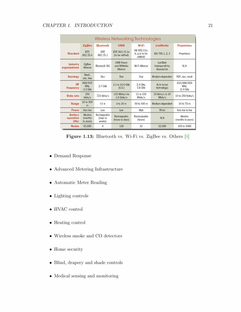
Figure 1.13: Bluetooth vs. Wi-Fi vs. ZigBee vs. Others [8]
• Demand Response
• Advanced Metering Infrastructure
• Automatic Meter Reading
• Lighting controls
• HVAC control
• Heating control
• Wireless smoke and CO detectors
• Home security
• Blind, drapery and shade controls
• Medical sensing and monitoring

CHAPTER 1. INTRODUCTION 22
• Remote control of home entertainment systems
• Indoor location sensing
• Advertising on mobile devices
The main trend in ZigBee development is improving power management and stack
interoperability. These features are called Smart Energy 2.0 (effort was launched in
2008 to offer IP-based HAN functionality).
1.5.5 The Concept of Open-Loop Control (OLC) and Closed-
Loop Control (CLC)
An open-loop controller, also called a non-feedback controller, is a type of controller
that computes its input into a system using only the current state and its model of
the system. The open-loop system is also called manual control system, see Figure
1.14.
A characteristic of the open-loop controller is that it does not use feedback to
determine if its output has achieved the desired goal of the input. Thus the system
does not observe the output of the processes that it is controlling. Consequently, a
true open-loop system cannot engage in machine learning and also cannot correct any
potential errors. It also compensate for disturbances in the system.
An open-loop controller is often used in simple processes because of its simplicity
and low cost, especially in systems where feedback is not critical. A typical example
would be a conventional washing machine, for which the length of machine wash time
is entirely dependent on the judgement and estimation of the human operator. In a
smart home, the open-loop controller can be used in some cases. The users can adjust
themselves to operate their smart appliances or by not tracking the instant price. The
CHAPTER 1. INTRODUCTION 23
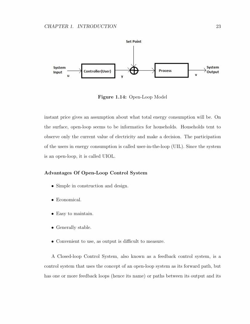
Figure 1.14: Open-Loop Model
instant price gives an assumption about what total energy consumption will be. On
the surface, open-loop seems to be informatics for households. Households tent to
observe only the current value of electricity and make a decision. The participation
of the users in energy consumption is called user-in-the-loop (UIL). Since the system
is an open-loop, it is called UIOL.
Advantages Of Open-Loop Control System
• Simple in construction and design.
• Economical.
• Easy to maintain.
• Generally stable.
• Convenient to use, as output is difficult to measure.
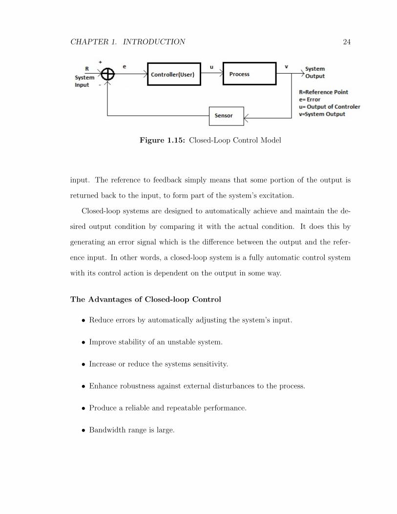
A Closed-loop Control System, also known as a feedback control system, is a
control system that uses the concept of an open-loop system as its forward path, but
has one or more feedback loops (hence its name) or paths between its output and its
CHAPTER 1. INTRODUCTION 24
Figure 1.15: Closed-Loop Control Model
input. The reference to feedback simply means that some portion of the output is
returned back to the input, to form part of the system’s excitation.
Closed-loop systems are designed to automatically achieve and maintain the de-
sired output condition by comparing it with the actual condition. It does this by
generating an error signal which is the difference between the output and the refer-
ence input. In other words, a closed-loop system is a fully automatic control system
with its control action is dependent on the output in some way.
The Advantages of Closed-loop Control
• Reduce errors by automatically adjusting the system’s input.
• Improve stability of an unstable system.
• Increase or reduce the systems sensitivity.
• Enhance robustness against external disturbances to the process.
• Produce a reliable and repeatable performance.
• Bandwidth range is large.

CHAPTER 1. INTRODUCTION 25
While a good closed-loop system can have many advantages over an open-loop
control system, its main disadvantage is that in order to provide the required amount
of control, a closed-loop system must be more complex by having one or more feedback
paths. Also, if the gain of the controller is too sensitive to changes in its input
commands or signals, it can become unstable and start to oscillate as the controller
tries to over-correct itself, and eventually risking it breaking. So we need to tell the
system how we want it to behave within some predefined limits.
Our system model is both an open-loop and closed-loop for UIL systems. In
an open-loop system the users are not supposed to give any feedback to the utility
company about their energy usage. However, the users can affect the whole system by
delaying their usage. Users are important active parameters that have initial impact
on the energy and money saving model. By looking at the users’ demands, the utility
company can adjust the production accordingly. Users make decisions after energy
generation beyond a short time; this may not be effective for energy saving purposes.
On the other hand, there is still something to do for demand shaping ideas. The
average energy usage of almost all types of appliances are similar. Assuming that
a washing machine usual time is 2 hours, utility companies can estimate how much
energy is using and how long it will continue. This is a classic approach, however
when it comes to millions of people’s applications, it is difficult to apply. Likewise,
most people prefer to use their appliances in their free time when the electricity price
may harm their budget.
An approach to change users’ decisions in terms of using their electricity is to
encourage them to delay their usage to later time when the electricity price is lower
than the average. Users will get some benefits by doing this.
Closed-loop model is a more efficient way to achieve an energy saving goal. In
this way, users instantly connect to their utility company to recover the instant price.

CHAPTER 1. INTRODUCTION 26
By doing this, users are encouraged to manage their energy and use their appliances
during the time when the price is low. The system repeats itself to update the
electricity price instantly and give a quick and correct feedback to users. Users will
get benefits by doing this as well.
1.5.6 Problem Statement
• Why do we change pricing models from fixed to current?
Our goal is to encourage end users to be an important parameter of saving
energy and money by using UIL method. For the sake of this idea users are
supposed to postpone or delay their demand to a latter time. To do that there
must be a time that the base price of electricity is relatively lower than the
other times. In the fixed pricing model, we have a stable base price in the whole
year; therefore, UIL method cannot work in this pricing model. In the current
model, we have a partial dynamic pricing method; therefore, UIL concept can
be applied here. In the half of the day, the electricity base prices are under
the average. For this reason, to help users to save energy and money, current
pricing model can be used in stead of fixed pricing model.
• Why do we need a dynamic pricing model?
Current pricing model works better than the fixed pricing model. However, to
get precise results, we need a fully dynamic pricing model. By doing this, users
turn on their appliances during the low-peak interval. Users’ demands remain
same, but they shift the demands to a low peak hour. When the number of
users increase, the energy saving decrease due to the increment in the average
base price.

CHAPTER 1. INTRODUCTION 27
• Why do we use 5 minutes cycle?
To say our system is a full dynamic system and supply changes very fast due
do the fast demand response, we have to reduce the interval as much as we can.
For this purposes, we take 5 minutes interval. In the literature, this interval is
taken 1 hour but it may not give a precise results in terms of saving [30], [31].
• Why UIL is more suitable for 5G instead of 4G?
UIL method can work under in 4G and 5G technologies. Since 4G is already
existed and mature technology, setting up UIL method cannot be %100 percent
applicable in this technology. Instead of 4G, 5G offers a more application based
IoTs technology which may involve smart grid communications. Besides, 5G
as the first network designed to be scalable, versatile, and energy smart for the
hyper-connected internet of everything world. 5G networks will be faster and
a lot smarter. It is assumed that IoTs generate massive data which cause con-
gestion in network. 5G may deal with this congestion by offering heterogeneous
networks [32].
• Why do we use UIL method?
UIL method first used for networks and efficient results. We used the same idea
for energy grid to contribute in saving energy and money.
• Problem we have to solve
Regarding to above, we have to make the problem statement. We know that
users try to save their energy and money by reducing their demand. This may
work until a point, but it is not an effective way because the need for energy
increases day by day. Without decreasing the demand, users can reduce their
payment to energy by postponing their demand. Thanks to this method the
total supply and demand will converge. When the supply and demand converged

CHAPTER 1. INTRODUCTION 28
with each other, in the big picture, the total supply will be reduced (shaped
based on the demand). In other words, utilities generate energy based on users
demand.
1.5.7 Contributions
After all, we can say that by setting up such systems and using UIL method, users save
both energy and money. These methods can be integrated to 5G technology easily.
We developed a dynamic pricing model with UIL method. We have used existing
technologies effectively such as ZegBee, smart meter, smart grid communications,
cellular networks, etc.
1.5.8 Thesis Organization
In Chapter 1, we introduce the base technologies that we use in our system model.
In Chapter 2, we summarized our system models and compared some existing tech-
nologies with our model. In addition we set up our ideas with different research areas.
In Chapter 3, we built an open-loop control model. In this model, we compared 3
different pricing models with or without the UIL method.
In Chapter 4, we built a closed loop control model rather than open-loop control. In
this model, we compared 3 different pricing models with or without the UIL method.
In Chapter 5, we analysed the results and make some statistical assumptions based
on these results.
Chapter 2
System Definition
The systems we proposed are both open-loop and closed-loop. We have compared
three type of pricing models are used in literature.
2.1 Pricing Systems Comparisons
2.1.1 Fixed Pricing Model
The fixed pricing model is still in use in various countries. In this system, the base
pricing method is totally different than the current pricing systems. The base price
remains stable during the whole year; the change in the price is only adjusted once
a year based on the inflation rate, smart meter charge, and other similar factors. In
other words, it does not matter how much energy the consumers try to save or thereby
contributing to the system for environmentally friendly purposes; the base price will
remain the same. Moreover, this system is concrete; there is no short time control on
the system on the end users side. Therefore, most of the time supply and demand do
not converge as seen in Figure 2.1. Supply and demand indicates electricity energy
in our system model.
29

CHAPTER 2. SYSTEM DEFINITION 30
Figure 2.1: Demand and Supply[8]
To meet the market demand, supply must be higher than demand in the most
circumstances. Figure 2.2 shows the relation between supply and demand.
P ∗ is the optimum price in which supply and demand exactly match with each
other. Q∗ is quantity of the demand and supply where both are equal each other.
Our goal is to provide this equilibrium in our system.
2.1.2 Current Pricing Model (Partly Dynamic)
Current pricing models are used in many countries such as Canada, United States
and Turkey. This pricing model is partially dynamic, which is better than the fixed
pricing model. If users have a smart meter installed in their house, the utility can
charge varying rates throughout the day, as seen in Figure 2.3. These rates are divided
into three separate bands known as off-peak, mid-peak and on-peak.
This pricing model gives ideas to the end users whether it would be suitable time
to turn on their appliances based on peak hour estimates. As a result of this time

CHAPTER 2. SYSTEM DEFINITION 31
Figure 2.2: Supply-Demand-Price Relation [9]
distinction, users are able to estimate how much energy they consume and what will
be the total price at end of each month. By knowing price ranges in advance, users
can adjust their demand to save money or energy.
2.1.3 Dynamic Pricing Model
The dynamic pricing model promises a development to address the concern of finding
an environmentally friendly solution of meeting energy demands so as to reduce cus-
tomer monthly bills. This type of model is not currently in use. This system enables
a fast communication between users and the utility companies. In each 5 minutes
circle, users send feedback message to supplier to shape the supply. For this purpose,
if end users shift their demand to a later time, they take the advantage of using
electricity in off-peak hours without changing their total demand. In other words,

CHAPTER 2. SYSTEM DEFINITION 32
Figure 2.3: On-Off-Peak Hours for Ontario [10]
CHAPTER 2. SYSTEM DEFINITION 33
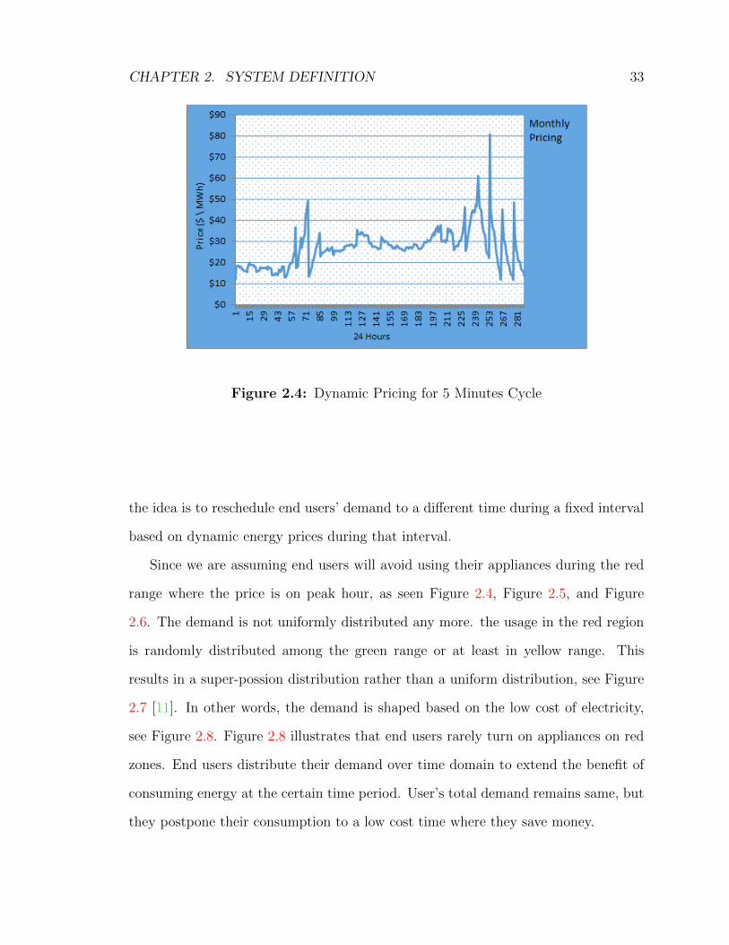
Figure 2.4: Dynamic Pricing for 5 Minutes Cycle
the idea is to reschedule end users’ demand to a different time during a fixed interval
based on dynamic energy prices during that interval.
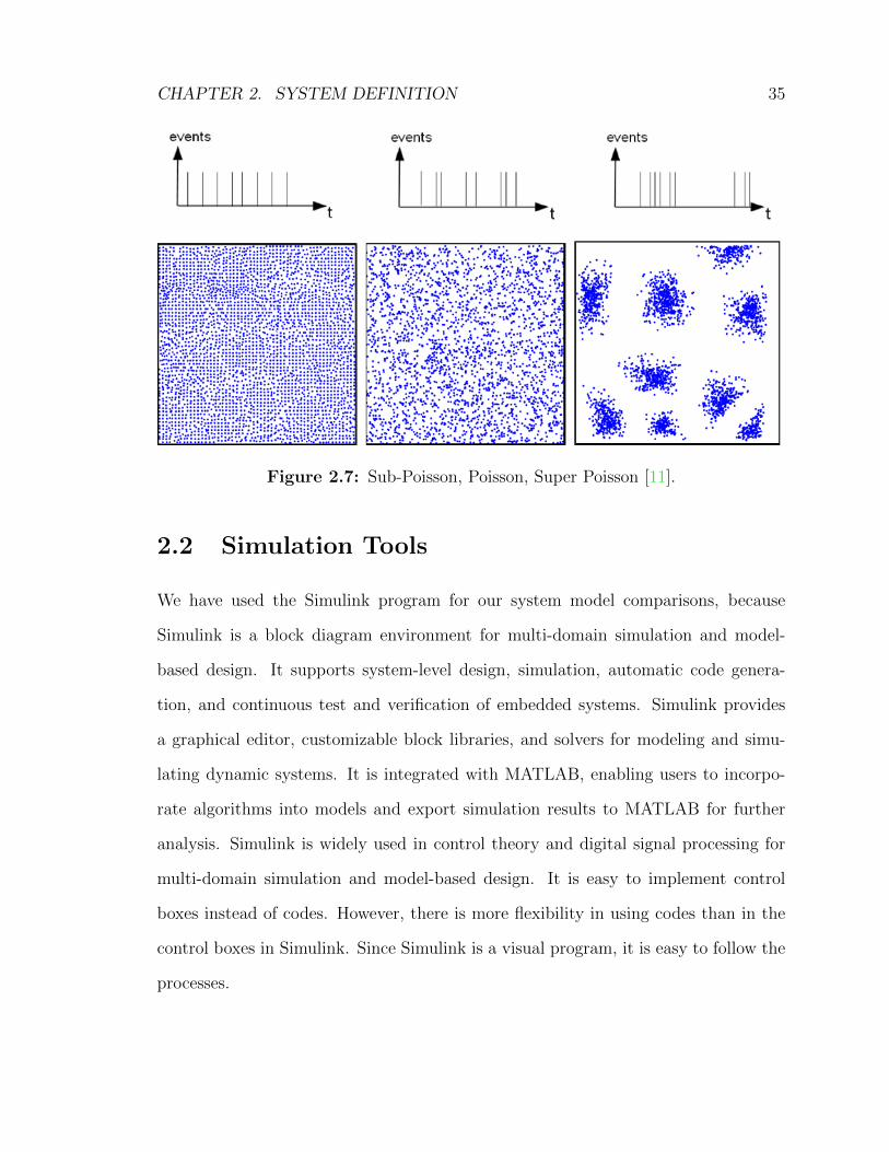
Since we are assuming end users will avoid using their appliances during the red
range where the price is on peak hour, as seen Figure 2.4, Figure 2.5, and Figure
2.6. The demand is not uniformly distributed any more. the usage in the red region
is randomly distributed among the green range or at least in yellow range. This
results in a super-possion distribution rather than a uniform distribution, see Figure
2.7 [11]. In other words, the demand is shaped based on the low cost of electricity,
see Figure 2.8. Figure 2.8 illustrates that end users rarely turn on appliances on red
zones. End users distribute their demand over time domain to extend the benefit of
consuming energy at the certain time period. User’s total demand remains same, but
they postpone their consumption to a low cost time where they save money.

CHAPTER 2. SYSTEM DEFINITION 34
Figure 2.5: Green-Yellow-Red Regions for Illinois
Figure 2.6: Green-Yellow-Red Regions for Ontario
CHAPTER 2. SYSTEM DEFINITION 35
Figure 2.7: Sub-Poisson, Poisson, Super Poisson [11].
2.2 Simulation Tools
We have used the Simulink program for our system model comparisons, because
Simulink is a block diagram environment for multi-domain simulation and model-
based design. It supports system-level design, simulation, automatic code genera-
tion, and continuous test and verification of embedded systems. Simulink provides
a graphical editor, customizable block libraries, and solvers for modeling and simu-
lating dynamic systems. It is integrated with MATLAB, enabling users to incorpo-
rate algorithms into models and export simulation results to MATLAB for further
analysis. Simulink is widely used in control theory and digital signal processing for
multi-domain simulation and model-based design. It is easy to implement control
boxes instead of codes. However, there is more flexibility in using codes than in the
control boxes in Simulink. Since Simulink is a visual program, it is easy to follow the
processes.

CHAPTER 2. SYSTEM DEFINITION 36
Figure 2.8: Air Conditioner
CHAPTER 2. SYSTEM DEFINITION 37
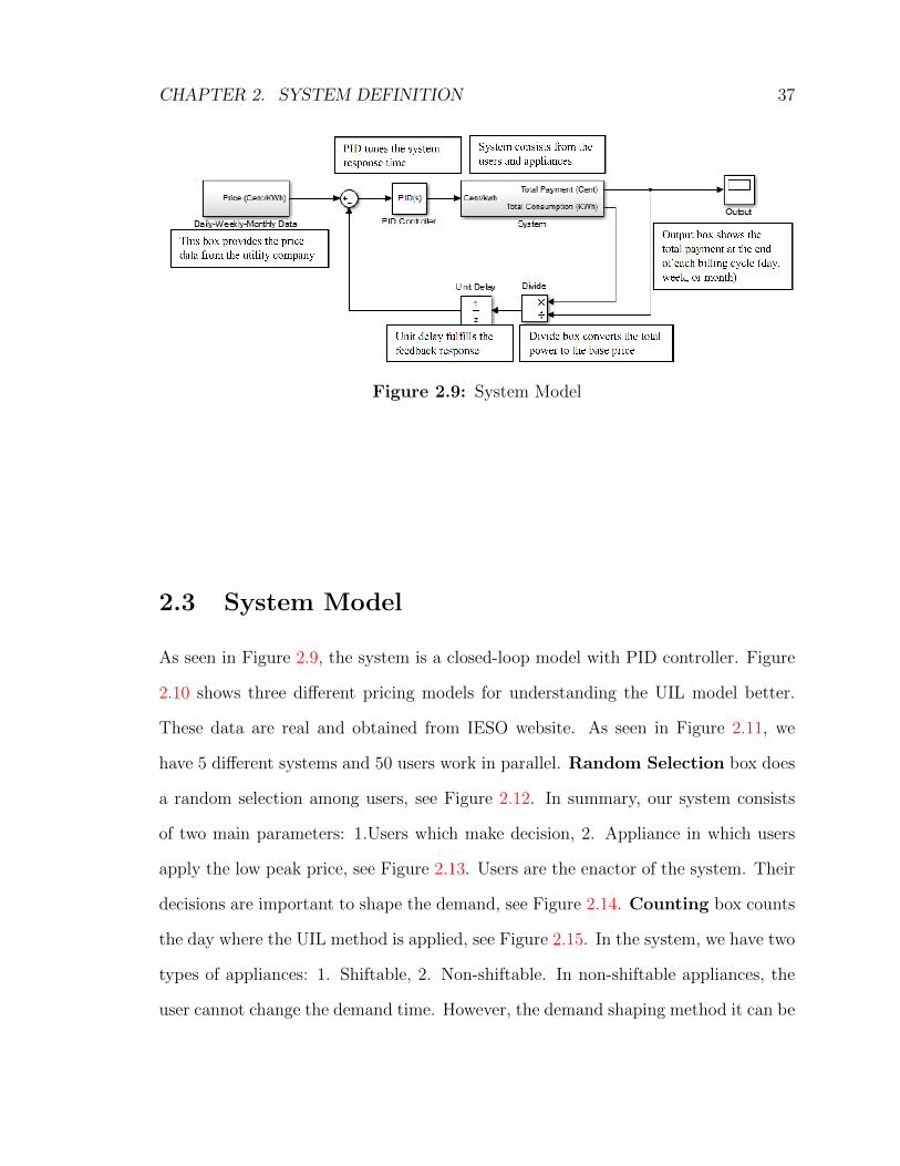
Figure 2.9: System Model
2.3 System Model
As seen in Figure 2.9, the system is a closed-loop model with PID controller. Figure
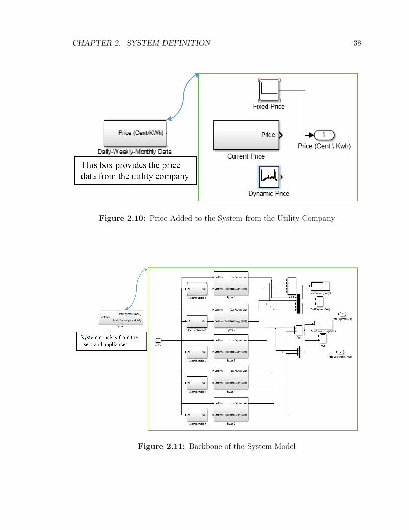
2.10 shows three different pricing models for understanding the UIL model better.
These data are real and obtained from IESO website. As seen in Figure 2.11, we
have 5 different systems and 50 users work in parallel. Random Selection box does
a random selection among users, see Figure 2.12. In summary, our system consists
of two main parameters: 1.Users which make decision, 2. Appliance in which users
apply the low peak price, see Figure 2.13. Users are the enactor of the system. Their
decisions are important to shape the demand, see Figure 2.14. Counting box counts
the day where the UIL method is applied, see Figure 2.15. In the system, we have two
types of appliances: 1. Shiftable, 2. Non-shiftable. In non-shiftable appliances, the
user cannot change the demand time. However, the demand shaping method it can be
CHAPTER 2. SYSTEM DEFINITION 38
Figure 2.10: Price Added to the System from the Utility Company
Figure 2.11: Backbone of the System Model

CHAPTER 2. SYSTEM DEFINITION 39
Figure 2.12: Random Selection Among Users
Figure 2.13: Main parameter of the System
CHAPTER 2. SYSTEM DEFINITION 40
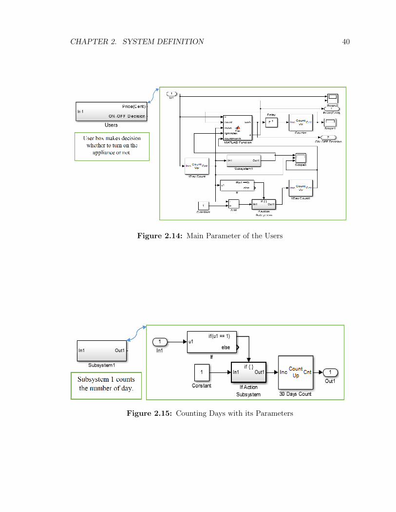
Figure 2.14: Main Parameter of the Users
Figure 2.15: Counting Days with its Parameters
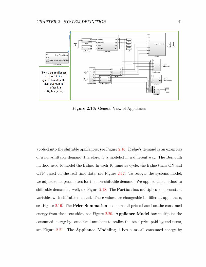
CHAPTER 2. SYSTEM DEFINITION 41
Figure 2.16: General View of Appliances
applied into the shiftable appliances, see Figure 2.16. Fridge’s demand is an examples
of a non-shiftable demand; therefore, it is modeled in a different way. The Bernoulli
method used to model the fridge. In each 10 minutes cycle, the fridge turns ON and
OFF based on the real time data, see Figure 2.17. To recover the systems model,
we adjust some parameters for the non-shiftable demand. We applied this method to
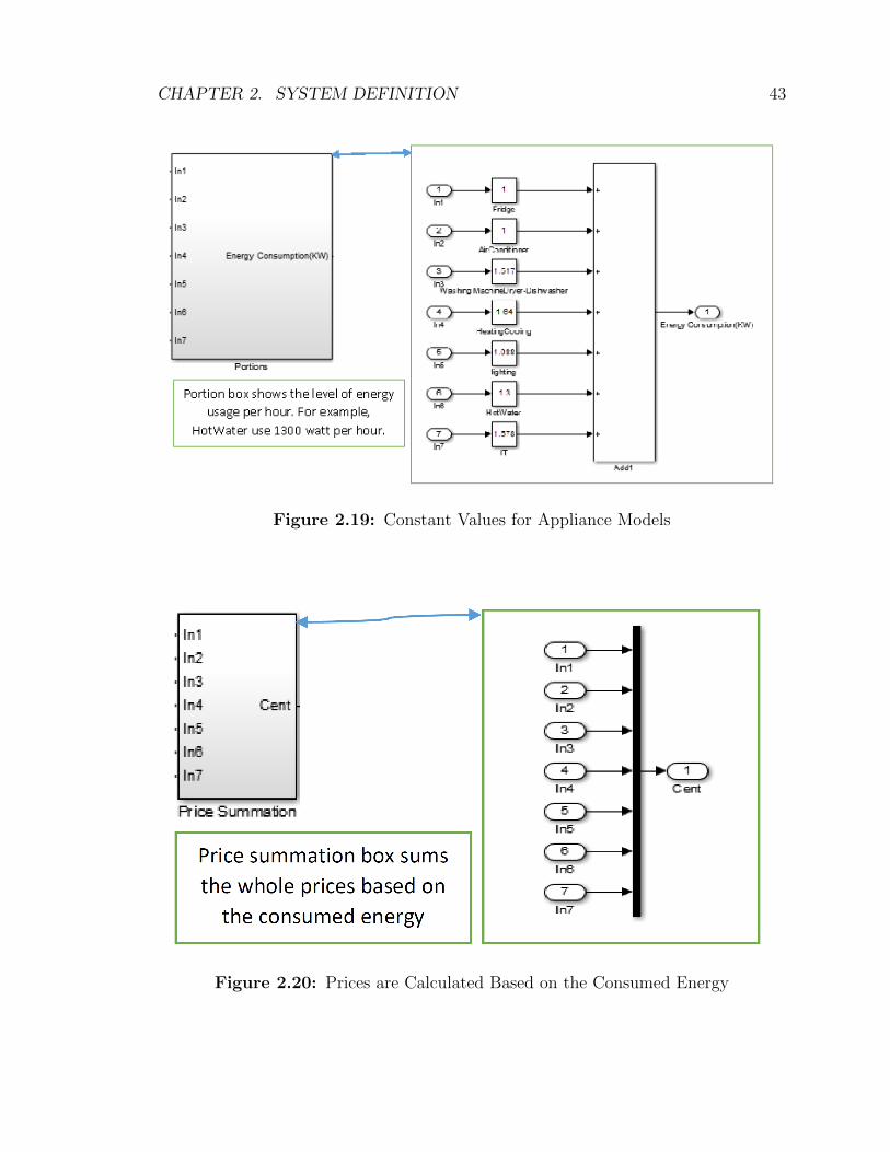
shifitable demand as well, see Figure 2.18. The Portion box multiplies some constant
variables with shiftable demand. These values are changeable in different appliances,
see Figure 2.19. The Price Summation box sums all prices based on the consumed
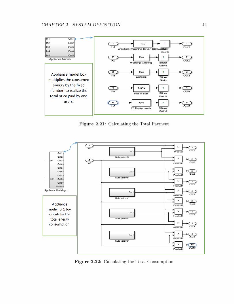
energy from the users sides, see Figure 2.20. Appliance Model box multiplies the
consumed energy by some fixed numbers to realize the total price paid by end users,
see Figure 2.21. The Appliance Modeling 1 box sums all consumed energy by

CHAPTER 2. SYSTEM DEFINITION 42
Figure 2.17: Fridge is an Example of non-Shiftable Demand
Figure 2.18: The Recover Parameters for non-Shiftable Demand
CHAPTER 2. SYSTEM DEFINITION 43
Figure 2.19: Constant Values for Appliance Models
Figure 2.20: Prices are Calculated Based on the Consumed Energy
CHAPTER 2. SYSTEM DEFINITION 44
Figure 2.21: Calculating the Total Payment
Figure 2.22: Calculating the Total Consumption

CHAPTER 2. SYSTEM DEFINITION 45
appliances in the user side, see Figure 2.22.
2.4 Independent Electricity System Operator
(IESO)
The Independent Electricity System Operator (IESO) works at the heart of Ontario’s
power system. It ensures whether or not there is enough power to meet the province’s
energy needs in real time. Moreover, IESO is planning and securing energy for the
future. It does this by:
• Balancing the supply of and demand for electricity in Ontario and directing its
flow across the province’s transmission lines.
• Planning for the province’ medium and long-term energy needs and securing
clean sources of supply to meet those needs.
• Overseeing the electricity wholesale market where the price is set.
• Fostering the development of a conservation culture in the province through
programs such as saveONenergy.
Ontario’s IESO works to ensure sufficient electricity is available whenever and
wherever it’s needed. Ensuring there is enough energy to meet demand is an ongoing
and highly complex process, requiring the close coordination of all parts of the system.
Every five minutes, the IESO forecasts electricity demand throughout the province
and directs generators to provide the required amount of electricity to meet that
demand. It can also reduce demand by calling on large volume users to cut back on
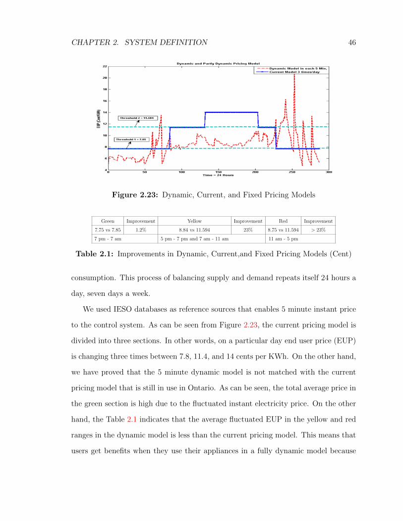
CHAPTER 2. SYSTEM DEFINITION 46
Figure 2.23: Dynamic, Current, and Fixed Pricing Models
Green Improvement Yellow Improvement Red Improvement
7.75 vs 7.85 1.2% 8.84 vs 11.594 23% 8.75 vs 11.594 > 23%
7 pm - 7 am 5 pm - 7 pm and 7 am - 11 am 11 am - 5 pm
Table 2.1: Improvements in Dynamic, Current,and Fixed Pricing Models (Cent)
consumption. This process of balancing supply and demand repeats itself 24 hours a
day, seven days a week.
We used IESO databases as reference sources that enables 5 minute instant price
to the control system. As can be seen from Figure 2.23, the current pricing model is
divided into three sections. In other words, on a particular day end user price (EUP)
is changing three times between 7.8, 11.4, and 14 cents per KWh. On the other hand,
we have proved that the 5 minute dynamic model is not matched with the current
pricing model that is still in use in Ontario. As can be seen, the total average price in
the green section is high due to the fluctuated instant electricity price. On the other
hand, the Table 2.1 indicates that the average fluctuated EUP in the yellow and red
ranges in the dynamic model is less than the current pricing model. This means that
users get benefits when they use their appliances in a fully dynamic model because
CHAPTER 2. SYSTEM DEFINITION 47
the real time price (in 5 minute cycle) is less than the current price. Currently, users
pay according to the current pricing model. On the contrary, when end users turn
on their appliances in the yellow or red ranges based on the current pricing model,
they have to pay higher than usual because real time pricing is less than the current
pricing model.
2.5 Summary of This Chapter
Our goal is to encourage end users to be aware of the high electricity prices when
it is higher than the regular constructed price. Since, end users avoid turning on
their appliances at the high priced time, based on supply-demand relation, the peak
price goes down and leads to a more smooth and efficient pricing range. In case of
congestion in demand after a point, end users are supposed to apply their demand to
block the intensity.

Chapter 3
Open-Loop Control Model
Open-loop control model doesn’t have any feedback to determine whether its output
has achieved the desired goal of the input. An electric clothes dryer would be a good
example of a device having an open-loop mechanism. Depending on the amount of
clothes or how wet they are, a user would set the timer (controller) of dryer as 30
minutes. 30 minutes later the dryer would automatically stop, even if the clothes
were still wet or damp, see Figure 3.1.
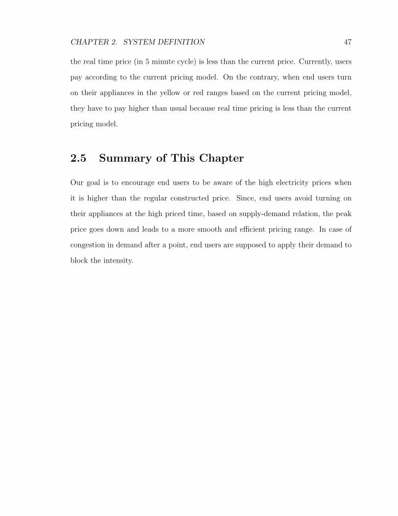
For an open-loop control (OLC) model, we have examined UIL under three types
of pricing models (fixed, current, and dynamic) in terms of the number of users and
appliances, see Figure 3.2.
Figure 3.1: Example for Open-Loop Control Model
48
CHAPTER 3. OPEN-LOOP CONTROL MODEL 49
Figure 3.2: Open-Loop Control Model Road Map

CHAPTER 3. OPEN-LOOP CONTROL MODEL 50
3.1 Fixed Pricing Model
In fixed pricing model, the EU price remains stable during the whole year. Therefore,
users cannot obtain any benefit such as saving money. In other words, end users
pay depending on their usage, see Figure 3.3. Therefore, there is a direct rela-
tionship between the total usage and the total payment as seen in the equation below:
Yi = α + βi ∗Xi
i = 1, 2, ...,
α = constant variable
β = independent variable
In the above, Yi is the total price in which end users pay for a one time turning
on their appliance; Xi
is the base price that is calculated from the supply-demand
relation. Then, α is a constant variable extracted from the inflation rate, interest
charges, distribution fees, smart meter charge, etc. Likewise, β refers to how long the
electricity has been used.
In the following subsections, I will explore fixed pricing model regarding the num-
ber of users and appliances.
3.1.1 One-User One-Appliance Model
Through this model, the demand for electricity is shifted in time domain because
there is a positive relationship between demand and price. Since end user price
remains stable during the whole year, there is no need for a threshold value for
this model. Since we have only one single user and only one single appliance, the
distribution of the demand changes based on user’s need for energy. Hence,
CHAPTER 3. OPEN-LOOP CONTROL MODEL 51
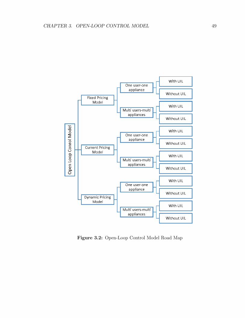
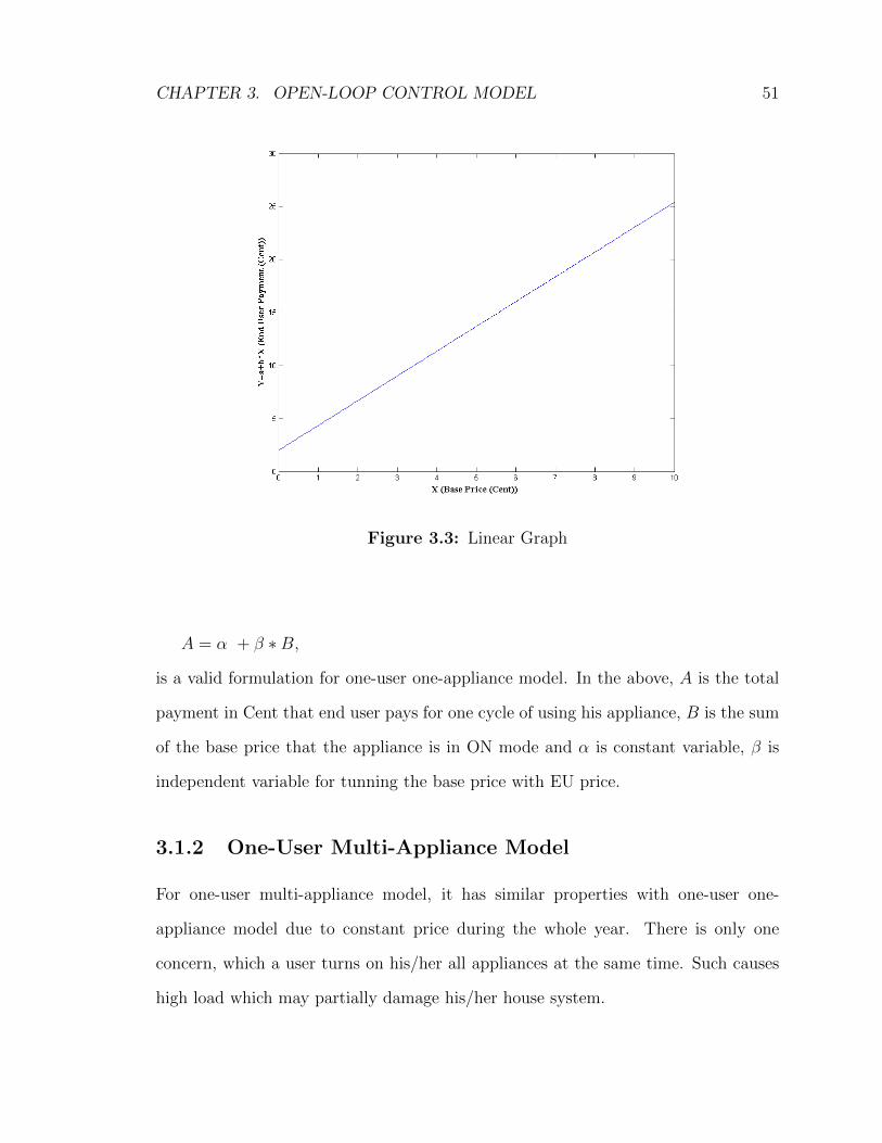
Figure 3.3: Linear Graph
A = α + β ∗B,
is a valid formulation for one-user one-appliance model. In the above, A is the total
payment in Cent that end user pays for one cycle of using his appliance, B is the sum
of the base price that the appliance is in ON mode and α is constant variable, β is
independent variable for tunning the base price with EU price.
3.1.2 One-User Multi-Appliance Model
For one-user multi-appliance model, it has similar properties with one-user one-
appliance model due to constant price during the whole year. There is only one
concern, which a user turns on his/her all appliances at the same time. Such causes
high load which may partially damage his/her house system.
CHAPTER 3. OPEN-LOOP CONTROL MODEL 52
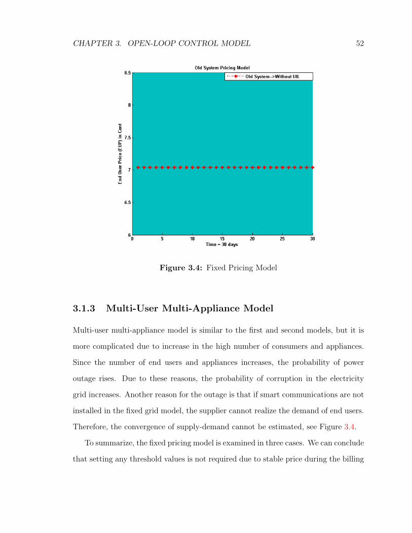
Figure 3.4: Fixed Pricing Model
3.1.3 Multi-User Multi-Appliance Model
Multi-user multi-appliance model is similar to the first and second models, but it is
more complicated due to increase in the high number of consumers and appliances.
Since the number of end users and appliances increases, the probability of power
outage rises. Due to these reasons, the probability of corruption in the electricity
grid increases. Another reason for the outage is that if smart communications are not
installed in the fixed grid model, the supplier cannot realize the demand of end users.
Therefore, the convergence of supply-demand cannot be estimated, see Figure 3.4.
To summarize, the fixed pricing model is examined in three cases. We can conclude
that setting any threshold values is not required due to stable price during the billing

CHAPTER 3. OPEN-LOOP CONTROL MODEL 53
period. Additionally, UIL method is not applicable because of undefined threshold
values.
3.2 Current Pricing Model
In the current pricing model, three time scales (green, yellow, and red ranges) are used
to settle the best convergence of supply and demand. When the difference between
supply and demand is low, it means the base price goes down, until point α. Likewise,
if the difference between supply and demand is high, the base price goes up, to a high
point. At this point, the supply side has to converge with demand; otherwise, neither
the base price (end user price) goes down, nor the goal of energy saving is reached.
Unlike the fixed pricing model, current pricing model is analyzed with respect to
only multi-user multi-appliance model because this pricing model is presently used
for a large number of users and appliances.
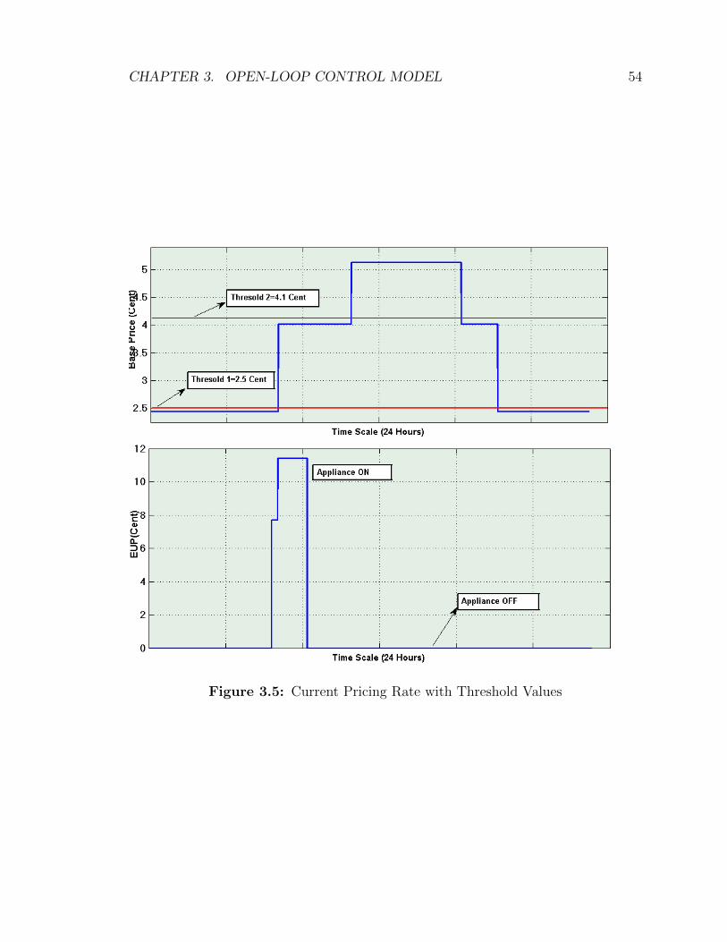
Defining Threshold Values
Threshold values are calculated based on the probability of the three different pricing
scales in which the base price and end user price are identified. We proposed that
end users operate their appliances when the base price is under τ1. This means that
during the green scale, which is already priced by the Energy Board of Ontario, users
are supposed to be in this scale. This has some benefits to end users; for instance
they have an opportunity to turn on their appliances in low price range, see Figure
3.5.
A probability density function is most commonly associated with absolutely
continuous univariate distributions. A random variable X has density fX , where fX
CHAPTER 3. OPEN-LOOP CONTROL MODEL 54
Figure 3.5: Current Pricing Rate with Threshold Values

CHAPTER 3. OPEN-LOOP CONTROL MODEL 55
Figure 3.6: PDF, CDF and Histogram of X (Base Price)

CHAPTER 3. OPEN-LOOP CONTROL MODEL 56
is a non-negative Lebesgue-integrable function, if
P [a ≤ X ≤ b] =∫ bafX(x)dx.
Hence, if fX is the cumulative distribution function of x, then
FX(x) =∫ x−∞ fX(u)du.
If fX is continuous at x
fX(x)dx = ddxFX(x).
As can be seen from Figure 3.6, the PDF of base price is different from regu-
lar PDFs. This results from different price scales that change during the day. On
the other hand, we understand that 36.4% of prices are in the green range while it
is 57% in yellow and 6.6% in the red range. However, Hydro Ottawa offers that
50% of prices are in the green range while it is 25% in yellow and 25% in the red
ranges. It can be clearly realized that the current pricing model that this company
suggests does not indicate the real pricing scale. This is resulted from an unstable
relation between the supply and demand curves. If this balance breaks down, the
price goes up or down. Next,this problem is associated with instant changes in
energy consumption and generation. We know that the alternative current (ac)
energy cannot be stored. Energy consumption and generation has to be done at the
same time. Energy demand changes very fast; therefore, the supply does not meet
the demand. This is the last reason for breaking down the supply - demand balance.
If suppliers are not ready for instant change on the demand side, basically, the power

CHAPTER 3. OPEN-LOOP CONTROL MODEL 57
systems can be damaged (costs billions of dollars) due to short cuts or other factors
caused from this short cuts.
To prevent these problems, we have to define two different threshold values based
on the CDF and PDF of the instant base prices. These threshold values help us to
limit the price range regarding to its value, for instance,
Set τ1 = 2.5, Cents
Set τ2 = 4.1, Cents
as shown in Figure 3.6
In the below we give a basic algorithm of making the best decision about time to turn
on the appliance:
Algorithm 1
if
BasePrice ≤ τ1
PrON = 1.0, P rOFF = 0.0
else if
τ1 ≤ Base Price ≤ τ2
PrON = 0.5, P rOFF = 0.5
else
BasePrice > τ2
PrON = 0.0, P rOFF = 1.0
end
Similarly, we can emerge end user price (EUP) based on these threshold values shown
in the below. Our threshold estimation is as follows:

CHAPTER 3. OPEN-LOOP CONTROL MODEL 58
EUP = 2 + 2.34 ∗BasePrice
for τ1
EUP1 = 7.8 Cents
for τ2
EUP2 = 11.6 Cents.
In the above, EUP1 and EUP2 define end user payment limits and range prices
respectively in three different colours (green, yellow, and red). Similar to Algorithm
1, we can define the Algorithm 2 that is already identified by HydroOttawa. Based
on the Algorithm 2, the EUP1 shows the bound of green and yellow ranges while
EUP2 shows the bound between yellow and red ranges. In the current pricing model,
EUPC1 is equal to 7.7 Cents and EUPC2 is equal to 11.4 Cents. It can be seen that
our estimation matches the current pricing model. In other words, these threshold
value estimations can be applied to dynamic pricing model.
Algorithm 2
if
BasePrice ≤ EUPC1
PrON = 1.0, P rOFF = 0.0
else if
EUPC1 < BasePrice ≤ EUPC2
PrON = 0.5, P rOFF = 0.5
else
BasePrice > EUPC2
PrON = 0.0, P rOFF = 1.0
end

CHAPTER 3. OPEN-LOOP CONTROL MODEL 59
Figure 3.7: One-User One-Appliance Model
The simulation of the current model for a different number of users and appliances
is shown in Figure 3.7.
When we use the UIL method in one-user one-appliance model, users reduce total
price for 10% by comparing the system without using UIL method. Similarly, for
multi-users multi-appliance, users still save money, around 5%. When the number of
users and appliances increase, using UIL partly lose its effectiveness. Since end users
turn on their appliances during low price time, they save money. Moreover system
gives information about the instant prices and avoid users be in high price time.
When the price is high users are supposed to adjust their demand to next time. As
can be seen from Figure 3.8, the appliance are not turned on in the red range where
is τ1=7.85 (Cents/KWh) for green range. On the other hand, when user doesn’t care

CHAPTER 3. OPEN-LOOP CONTROL MODEL 60
Figure 3.8: Multi-User Multi-Appliances Model
CHAPTER 3. OPEN-LOOP CONTROL MODEL 61
the usage, the base price may be higher than τ2= 11.4 (Cents/KWh) which is the
second limit yellow range.
To sum up,the current pricing model does not meet the real criteria, because
the base price is calculated instantly from the relation between supply and demand.
Instead of three times scaling, we offer a fully dynamic pricing model that meet our
criteria and works better than the current pricing model with the UIL method. When
we use UIL method in the current pricing model, users save money around 7.5% in
each billing period.
3.3 Dynamic Pricing Model
User in the loop (UIL) is the idea that end users are supposed to delay their usage
to a later time. By doing this, end user stays away from being in high price time.
The goal of UIL is to encourage end users to make an efficient decision in terms of
lower prices. For the open-loop system, end user is supposed to make a decision either
to turn on his appliance or not. However, this decision does not impact the input
variables. This means that, user makes a decision only of a suitable time to turn
on his smart appliances without any feedback to the supplier. In other words, the
open-loop model does not have any feedback; therefore, the impact of end user on
saving money is limited.
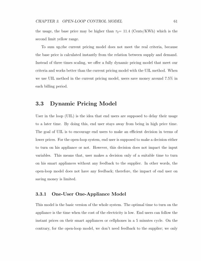
3.3.1 One-User One-Appliance Model
This model is the basic version of the whole system. The optimal time to turn on the
appliance is the time when the cost of the electricity is low. End users can follow the
instant prices on their smart appliances or cellphones in a 5 minutes cycle. On the
contrary, for the open-loop model, we don’t need feedback to the supplier; we only
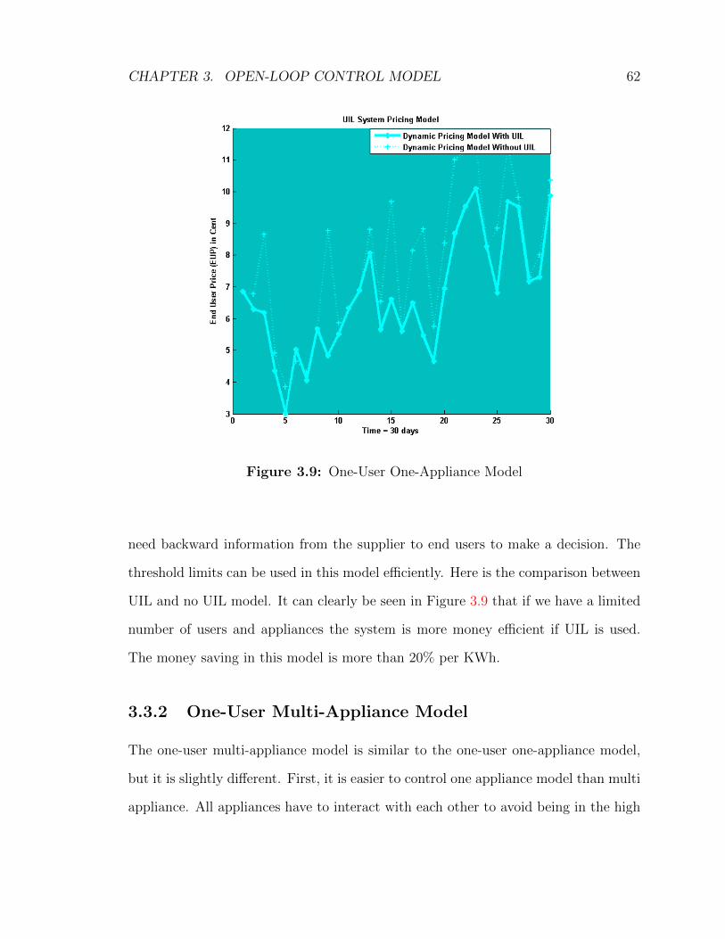
CHAPTER 3. OPEN-LOOP CONTROL MODEL 62
Figure 3.9: One-User One-Appliance Model
need backward information from the supplier to end users to make a decision. The
threshold limits can be used in this model efficiently. Here is the comparison between
UIL and no UIL model. It can clearly be seen in Figure 3.9 that if we have a limited
number of users and appliances the system is more money efficient if UIL is used.
The money saving in this model is more than 20% per KWh.
3.3.2 One-User Multi-Appliance Model
The one-user multi-appliance model is similar to the one-user one-appliance model,
but it is slightly different. First, it is easier to control one appliance model than multi
appliance. All appliances have to interact with each other to avoid being in the high

CHAPTER 3. OPEN-LOOP CONTROL MODEL 63
cost range. To put it in other words, two appliances will not work at the same time.
The only concern is if the number of appliances in ON mode is high, it can damage
the house grid system.
3.3.3 Multi-User Multi-Appliance Model
Here is the complicated version of the whole model. If the system has many users,
it is going to be more complex because all users have to interact with each other
to prevent high load during the low cost time. Since the system is open-loop, it is
impossible to provide interconnection among the all users around the city to specify
the best time to turn on their appliances one by one. Here is the comparison of
multi-users multi-appliance model, see Figure 3.10. Since the number of users and
appliances is high we are not satisfied by using UIL method.
3.4 Summary of This Chapter
We built an open-loop control model. In this model, we analyzed UIL method under
3 different pricing models in terms of the number of users.
As a result, we understand that the UIL method enables efficient results for a
small number of users.

CHAPTER 3. OPEN-LOOP CONTROL MODEL 64
Figure 3.10: Multi-User Multi-Appliance Model
Chapter 4
Closed-Loop Control Model
A closed-loop control system is known as a feedback control system. Unlike the
open-loop control model, the closed-loop control model employs one or more feedback
mechanisms. The reference to feedback simply means that some portion of the output
is returned back to the input in order to form part of the systems excitation.
Closed-loop systems are designed to achieve and maintain the desired output
condition by comparing reference input with the real-time output. This comparison
is made through generating an error signal which indicates the difference between the
output and the reference input.
Closed-loop systems can be integrated into home appliances such as an electric
clothes dryer. Suppose that we have used a sensor or transducer input device) to
continually monitor the dryness of clothes. This sensor would monitor the actual
dryness of the clothes and compare it with (or subtract it from) the input refer-
ence. The error signal (error = required dryness actual dryness) is amplified by the
controller, and the controller output makes the necessary correction to the heating
system to reduce any error. For example, if the clothes are too wet the controller
may increase the temperature or drying time. Likewise, if the clothes are about to
dry, either the temperature can be reduced or the dryer maybe stopped the process
65

CHAPTER 4. CLOSED-LOOP CONTROL MODEL 66
Figure 4.1: Closed-Loop Models
to prevent overheating the clothes, etc. See Figure 4.1.
The closed-loop configuration is characterized by the feedback signal derived from
the sensor in clothes drying system. The magnitude and polarity of the resulting
error signal would be directly related to the difference between the referent dryness
and real-time dryness of the clothes.
When the deviation in temperature is detected by the feedback sensor and the
controller self-corrects the error to maintain a constant temperature within the limits
of the pre-set value, the dryer’s door is opened or heat is reduced. Or, possibly, stops
the process and activates an alarm to inform the operator.
As we can see, in a closed-loop control system the error signal is fed to the con-
troller so as to reduce the systems error and bring the output of the system back to a
desired value. Obviously, when the error is zero, the clothes are dry. Employing user
in the loop method in closed-loop model results in super-Poisson distribution rather
than uniform distribution. Therefore, relatively lower prices can be identified to meet
end users’ demand. In the UIL model, the controller is the proportional-integral-
derivative controller (PID controller), which controls the feedback loop mechanism
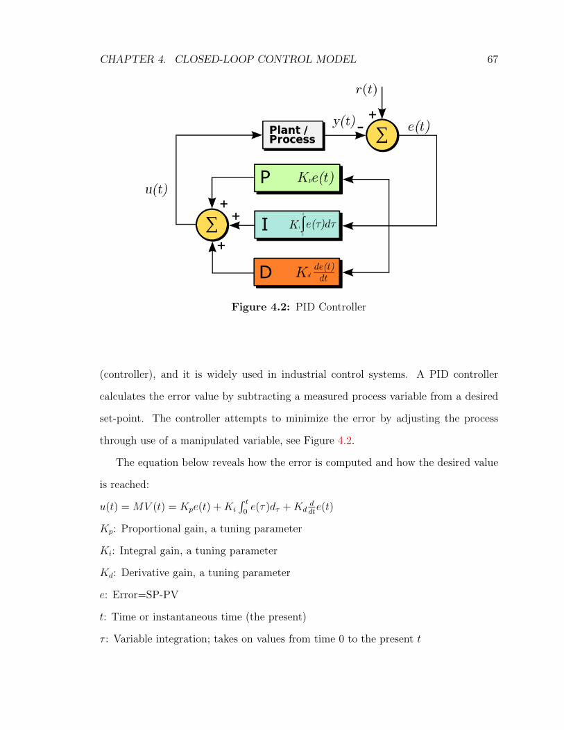
CHAPTER 4. CLOSED-LOOP CONTROL MODEL 67
Figure 4.2: PID Controller
(controller), and it is widely used in industrial control systems. A PID controller
calculates the error value by subtracting a measured process variable from a desired
set-point. The controller attempts to minimize the error by adjusting the process
through use of a manipulated variable, see Figure 4.2.
The equation below reveals how the error is computed and how the desired value
is reached:
u(t) = MV (t) = Kpe(t) +Ki
∫ t0e(τ)dτ +Kd
ddte(t)
Kp: Proportional gain, a tuning parameter
Ki: Integral gain, a tuning parameter
Kd: Derivative gain, a tuning parameter
e: Error=SP-PV
t: Time or instantaneous time (the present)
τ : Variable integration; takes on values from time 0 to the present t
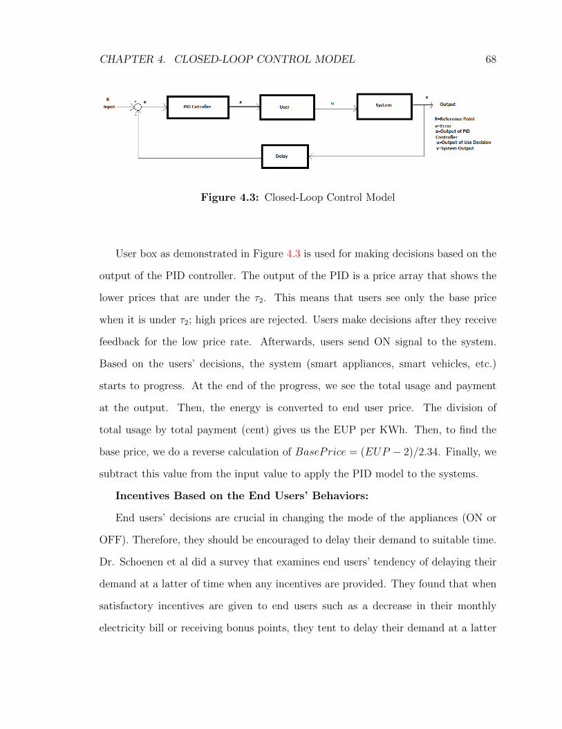
CHAPTER 4. CLOSED-LOOP CONTROL MODEL 68
Figure 4.3: Closed-Loop Control Model
User box as demonstrated in Figure 4.3 is used for making decisions based on the
output of the PID controller. The output of the PID is a price array that shows the
lower prices that are under the τ2. This means that users see only the base price
when it is under τ2; high prices are rejected. Users make decisions after they receive
feedback for the low price rate. Afterwards, users send ON signal to the system.
Based on the users’ decisions, the system (smart appliances, smart vehicles, etc.)
starts to progress. At the end of the progress, we see the total usage and payment
at the output. Then, the energy is converted to end user price. The division of
total usage by total payment (cent) gives us the EUP per KWh. Then, to find the
base price, we do a reverse calculation of BasePrice = (EUP − 2)/2.34. Finally, we
subtract this value from the input value to apply the PID model to the systems.
Incentives Based on the End Users’ Behaviors:
End users’ decisions are crucial in changing the mode of the appliances (ON or
OFF). Therefore, they should be encouraged to delay their demand to suitable time.
Dr. Schoenen et al did a survey that examines end users’ tendency of delaying their
demand at a latter of time when any incentives are provided. They found that when
satisfactory incentives are given to end users such as a decrease in their monthly
electricity bill or receiving bonus points, they tent to delay their demand at a latter
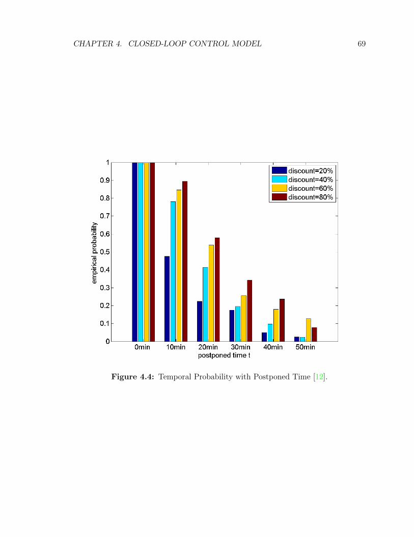
CHAPTER 4. CLOSED-LOOP CONTROL MODEL 69
Figure 4.4: Temporal Probability with Postponed Time [12].

CHAPTER 4. CLOSED-LOOP CONTROL MODEL 70
Figure 4.5: The Outline of Closed-Loop Control Model
of time, see Figure 4.4.
For a closed-loop control (CLC) model, we have examined the UIL method under
three types of pricing models (fixed, current, and dynamic) in terms of multi user-
multi appliance model, see Figure 4.5.
4.1 Fixed Pricing Model
Since the base price is stable during the whole year in the fixed pricing model, end
user cannot earn any benefits from it. Therefore, it doesn’t matter whether end users
are a part of the system or not, see Figure 4.6.

CHAPTER 4. CLOSED-LOOP CONTROL MODEL 71
Figure 4.6: Fixed Pricing System for Closed-Loop Model
4.2 Current Model
In the current model, if users are a part of the system they can obtain some advan-
tages. First, they can manage their usage depending on when the electricity price
is low. As seen in Figure 4.7, user’s payment doesn’t exceed τ2 value. Second, by
shaping their demand in time domain, they prevent high load congestion. Since they
shape their demands, they help to shape supply. As a result, the supply and demand
get closer to each other. Third, user awareness toward green energy increases.

CHAPTER 4. CLOSED-LOOP CONTROL MODEL 72
Figure 4.7: Current Pricing System for Closed-Loop Model
4.3 Dynamic Pricing Model
Threshold values are crucial in the dynamic pricing model, because the systems with-
out these values turn into regular systems that users cannot get any benefit. Cur-
rently, HydroOne does not provide such a system for its users.
In the UIL model, end users are assumed to make a quick decision based on the
relatively lower prices. In the closed-loop control model with the UIL model, the
EUP price goes down after τ1 and getting closer to α as seen in Figure 4.8.
4.4 Summary of This Chapter
The term of the closed-loop control always implies the use of a feedback control sensor
in order to determine and minimize the amount errors within the system.

CHAPTER 4. CLOSED-LOOP CONTROL MODEL 73
Figure 4.8: Dynamic Pricing System for Closed-Loop Model
In the closed-loop control model, we have examined the effectiveness of UIL
method on 3 different pricing model regarding multi-user multi-appliance. Chap-
ter 4 indicates that closed-loop control model is suitable for a large number of users
and appliances. On the other hand, if the number of users and appliances is fewer,
the number of low price periods increases.

Chapter 5
Conclusion and Future Works
In statistics, the coefficient of determination, denoted R2 and pronounced R squared,
is a number that indicates how well data fit a statistical model, sometimes simply a
line or curve. However, it is not necessary that the high value of R2 is good.
As seen from Figure 5.1 and Figure 5.2, there is a parallel relation between supply,
demand, and base price curves. This means that when the demand goes up, the supply
goes up. Then the price is adjusted based on this relation. However, this price is the
average of one month. When it comes to a one day relation, it is totally different.
We understand from demand and supply formula that the convergence between them
is more than 90%, while it is approximately 50% for the base price see Figure 5.3.
Therefore, it will be a good idea to compare the base price to supply and demand to
make a perfect realization.
5.1 Open-Loop Results
Here is the relation between all three kinds of pricing models with and without the
UIL method. In Figure 5.4, if we use the UIL method instead of the regular one, we
74
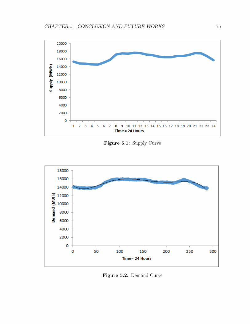
CHAPTER 5. CONCLUSION AND FUTURE WORKS 75
Figure 5.1: Supply Curve
Figure 5.2: Demand Curve

CHAPTER 5. CONCLUSION AND FUTURE WORKS 76
Figure 5.3: Electricity Price Distribution
basically save 23% in the current pricing model. A dynamic pricing model has more
than an 8% improvement when we use UIL in the total in Figure 5.5.
When the number of user and appliances increases we still save but not as high
as the one user-one appliance method.
5.2 Closed-Loop Results
In Chapter 4, we only simulated for multi-user multi-appliance. For the current
pricing model, the total saving is around 5%. Since we have used PID in closed-loop
controller, the error between EUP and feedback price is going down and reach to
zero. Total savings, for dynamic pricing, is about 7.5%. As can be seen from Figure
5.6, in a long period, in the dynamic pricing model, the UIL has higher advantages
than without using the UIL.

CHAPTER 5. CONCLUSION AND FUTURE WORKS 77
Figure 5.4: One-User One-Appliance
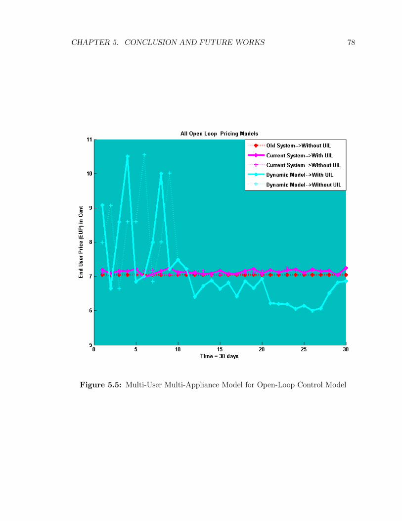
CHAPTER 5. CONCLUSION AND FUTURE WORKS 78
Figure 5.5: Multi-User Multi-Appliance Model for Open-Loop Control Model
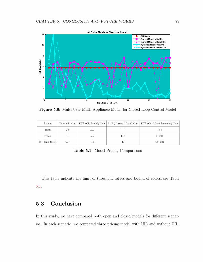
CHAPTER 5. CONCLUSION AND FUTURE WORKS 79
Figure 5.6: Multi-User Multi-Appliance Model for Closed-Loop Control Model
Region Threshold-Cent EUP (Old Model)-Cent EUP (Current Model)-Cent EUP (Our Model Dynamic)-Cent
green 2.5 9.97 7.7 7.85
Yellow 4.1 9.97 11.4 11.594
Red (Not Used) >4.1 9.97 14 >11.594
Table 5.1: Model Pricing Comparisons
This table indicate the limit of threshold values and bound of colors, see Table
5.1.
5.3 Conclusion
In this study, we have compared both open and closed models for different scenar-
ios. In each scenario, we compared three pricing model with UIL and without UIL.

CHAPTER 5. CONCLUSION AND FUTURE WORKS 80
Figure 5.7: Comparison of Simulated Models with Different Number of Users w/oUIL Method
Additionally, we did these simulations for both one-user one-appliance and multi-
user multi-appliance. From this thesis, we understood that UIL method works well
especially for a low number of user and appliances. When the number of user and
appliances increases, the total saving falls down slightly. In total, when users par-
ticipated to the system and started being an active energy saver by adjusting their
demand based on time and low price, they saved in energy and money. As a result,
suppliers do not need to generate extra energy. They start to generate according to
the demand from the consumers. There will be a tight interaction between consumer,
supplier, smart appliance and cellphones. We use two way communications both in
wire line and wireless.
Wireless communication is very important to set up such system, to communicate
fast. Users have to transmit their demand to the supplier in a very short period..
Likewise, ZegBee communication is important to set interaction between devices and
appliances.

CHAPTER 5. CONCLUSION AND FUTURE WORKS 81
5.3.1 Improvements Over the Current Pricing Model and Fu-
ture Works
• 7% − 11% money efficiency,
• 12% money efficiency from supplier side,
• 7.5% − 12.5% energy efficiency,
• Environmentally friendly, less CO emission,
• Increase end user awareness,
• Attention to renewable energy usage,
• More smart and safe system,
• Real time monitoring and reaction,
• Individual energy management,
• Prevention waste energy,
• Direct communication to end user customers,
• Maintain global competition.
We did limited research on smart grid communication; we did some assumptions
in some parameters. For a more realistic model:
• Human behaviours have to be understood for precise assumptions,
• Sensors and some statistical measurements can be used to realize the resultsm,
• Since the system needs hundreds of data, the ”Big Data” concept can be intro-
duced to the systems,

CHAPTER 5. CONCLUSION AND FUTURE WORKS 82
• Our system is good for a limited number of users and appliances; therefore
big data can be used to extend the model for millions of users, smart phones,
laptops and smart appliances,
• We have used real data for our system. However, in reality we don’t have
such data in advance. Therefore, some filter techniques could be used for base
price estimations. Kalman filters and the moving average (MA) method can be
integrated to this system for making electricity price assumptions.
List of References
[1] Y. Martel, “The internet of things.” http://www.opinno.com/en/content/
internet-things-0?language=es.[Accessed: 12- Feb- 2013].
[2] HydroOne, “Automated meter reading.” http://www.hydroone.com/
myhome/myaccount/mymeter/pages/automatedmeterreading.aspx [Accessed:
03- May- 2015].
[3] N. on the Lake Hydro, “Niagara on the lake.” http://www.notlhydro.com/
smartmeters/pricing [Accessed: 03- May- 2015].
[4] O. E. Board, “Electricity prices.” http://www.ontarioenergyboard.ca/OEB/
Consumers/Electricity/Electricity+Prices [Accessed: 03- May- 2015].
[5] R. Aulana, “Plc (power line communication).” http://rustammaulana.
blogspot.ca/2012/10/plc-power-line-communication.html.[Accessed: 05-
May- 2015].
[6] R. Schoenen and H. Yanikomeroglu, “Dynamic demand control with differenti-
ated qos in user-in-the-loop controlled cellular networks,” in IEEE 77th Vehicular
Technology Conference (VTC Spring), pp. 1–6, 2013.
[7] Kanda, “Zigbee wireless interfaces and products.” http://www.kanda.com/
zigbee-wireless.html [Accessed: 06- May- 2015].
[8] Electronicdesign, “Use zigbee for cost-effective wpan sensing and con-
trol solutions — proactive, logical, and well-organized design evaluation
with a solid reference design helps simplify wireless personal-area net-
works (wpan) design and development — communications content from
electronic design.” http://electronicdesign.com/communications/
use-zigbee-cost-effective-wpan-sensing-and-control-solutions
[Accessed: 06- May- 2015].
83
84
[9] Z. Economics, “Supply and demand.” https://zahablog.wordpress.com/
concepts/basics-and-markets/supply-and-demand-2.[Accessed: 03- May-
2015].
[10] O. Hydro, “Ontario time-of-use electricity rates.” http://www.ontario-hydro.
com/index.php?page=current_rates[Accessed: 03- May- 2015].
[11] M. Mirahsan, Z. Wang, R. Schoenen, H. Yanikomeroglu, and M. St-Hilaire, “Uni-
fied and non-parameterized statistical modeling of temporal and spatial traffic
heterogeneity in wireless cellular networks,” in IEEE International Conference on
Communications Workshops (ICC) 2014 Workshop on 5G Technologies, pp. 55–
60, 10-14 June 2014.
[12] R. Schoenen, G. Bulu, A. Mirtaheri, T. Beitelmal, and H. Yanikomeroglu, “First
survey results of quantified user behavior in user-in-the-loop scenarios for sus-
tainable wireless networks,” in IEEE Vehicular Technology Conference (VTC
Fall), pp. 1–5, 2012.
[13] J. Holler, V. Tsiatsis, C. Mulligan, S. Avesand, S. Karnouskos, and D. Boyle,
From Machine-to-machine to the Internet of Things: Introduction to a New Age
of Intelligence. Academic Press, 2014.
[14] E. Evolving, “Analytics, Machine Learning, and the Internet of Things,”
[15] A. B. Intelligence, “More than 30 billion devices will wirelessly connect to the
internet of everything in 2020,” ABI research news, vol. 9, 2013.
[16] N. Kushalnagar, G. Montenegro, C. Schumacher, et al., “Ipv6 over low-power
wireless personal area networks (6lowpans): overview, assumptions, problem
statement, and goals,” RFC4919, vol. 10, August 2007.
[17] R. Schoenen, G. Bulu, A. Mirtaheri, and H. Yanikomeroglu, “Green communi-
cations by demand shaping and user-in-the-loop tariff-based control,” in IEEE
Online Conference on Green Communications (GreenCom), pp. 64–69, 2011.
[18] I. Richardson, M. Thomson, D. Infield, and C. Clifford, “Domestic electricity
use: A high-resolution energy demand model,” Energy and Buildings, vol. 42,
no. 10, pp. 1878–1887, 2010.
[19] F. Rahimi and A. Ipakchi, “Demand response as a market resource under the
smart grid paradigm,” IEEE Transactions on Smart Grid, vol. 1, no. 1, pp. 82–
88, 2010.

85
[20] W. Li and X. Zhang, “Simulation of the smart grid communications: Challenges,
techniques, and future trends,” Computers & Electrical Engineering, vol. 40,
no. 1, pp. 270–288, 2014.
[21] M. Aydinalp, V. I. Ugursal, and A. S. Fung, “Modeling of the appliance, lighting,
and space-cooling energy consumptions in the residential sector using neural
networks,” Applied Energy, vol. 71, no. 2, pp. 87–110, 2002.
[22] H. Mouftah and M. Erol-Kantarci, “Smart grid communications: Opportu nities
and challenges,” Handbook on Green Communication and Systems, edited by MS
Obaidat, A. Anpalagan and I. Woungang, Wiley, 2012.
[23] A. Ghassemi, S. Bavarian, and L. Lampe, “Cognitive radio for smart grid com-
munications,” in IEEE First International Conference on Smart Grid Commu-
nications (SmartGridComm), pp. 297–302, 2010.
[24] D. Dzung, I. Berganza, and A. Sendin, “Evolution of powerline communica-
tions for smart distribution: from ripple control to OFDM,” in IEEE Inter-
national Symposium on Power Line Communications and Its Applications (IS-
PLC), pp. 474–478, 2011.
[25] Z. Wang, R. Schoenen, H. Yanikomeroglu, and M. St-Hilaire, “Load balancing in
cellular networks with user-in-the-loop: A spatial traffic shaping approach,” in
IEEE International Conference on Communications (ICC). London, UK, 2015.
[26] R. Schoenen and H. Yanikomeroglu, “User-in-the-loop: spatial and temporal de-
mand shaping for sustainable wireless networks,” IEEE Communications Maga-
zine, vol. 52, no. 2, pp. 196–203, 2014.
[27] R. Schoenen and H. Yanikomeroglu, “Erlang analysis of cellular networks using
stochastic petri nets and user-in-the-loop extension for demand control,” in IEEE
Globecom Workshops (GC Wkshps), pp. 298–303, 2013.
[28] R. Schoenen, G. Bulu, A. Mirtaheri, T. Beitelmal, and H. Yanikomeroglu,
“Quantified user behavior in user-in-the-loop spatially and demand controlled
cellular systems,” in European Wireless, 2012. EW. 18th European Wireless Con-
ference, pp. 1–8, 2012.
[29] T. Beitelmal, R. Schoenen, and H. Yanikomeroglu, “On the impact of corre-
lated shadowing on the performance of user-in-the-loop for mobility,” in IEEE
International Conference on Communications (ICC), pp. 7040–7044, 2012.

86
[30] J. H. Yoon, R. Baldick, and A. Novoselac, “Dynamic demand response controller
based on real-time retail price for residential buildings,” IEEE Transactions on
Smart Grid, vol. 5, no. 1, pp. 121–129, 2014.
[31] A. J. Conejo, J. M. Morales, and L. Baringo, “Real-time demand response
model,” IEEE Transactions on Smart Grid, vol. 1, no. 3, pp. 236–242, 2010.
[32] W. H. Chin, Z. Fan, and R. Haines, “Emerging technologies and research chal-
lenges for 5G wireless networks,” IEEE Wireless Communications, vol. 21, no. 2,
pp. 106–112, 2014.

Appendix A
Equations
Supply Formula:
y = −0.0031x6 +0.1743x5−2.9319x4 +3.7674x3 +277.09x2−1589.6x+16743(KWh)
R2 = 0.9489
Demand Formula:
y = (−1E − 07)x5 + 0.0001x4 − 0.0268x3 + 2.8439x2 − 91.905x+ 14541(KWh)
R2 = 0.9373
Price Distribution:
y = (−1E− 09)x5 + (7E− 07)x4 − 0.0002x3 + 0.0159x2 − 0.4658x+ 19.738 (Cent per
KWh)
R2 = 0.4793
87


![4. Demand Side Management in Smart Grid Using [Autosaved]](https://static.fdocuments.in/doc/165x107/55cf8e36550346703b8fc6f3/4-demand-side-management-in-smart-grid-using-autosaved.jpg)