Fast computation of Lyot-style coronagraph...

Fast computation of Lyot-stylecoronagraph propagation

R. Soummer∗1,2, L. Pueyo3,A. Sivaramakrishnan 1,2,4, and R. J. Vanderbei5

1Department of Astrophysics, American Museum of Natural History, New York, NY 100242 Center for Adaptive Optics, University of California, Santa Cruz, CA 95064

3Mechanical and Aerospace Engineering, Princeton University, Princeton, NJ 085444Department of Physics and Astronomy, Stony Brook University, Stony Brook, NY 11794

5Operations Research and Financial Engineering, Princeton University, Princeton, NJ 08544corresponding author:

[email protected]

Abstract: We present a new method for numerical propagations throughLyot-style coronagraphs using finite size occulting masks.Standard meth-ods for coronagraphic simulations involve Fast Fourier Transforms (FFT)of very large arrays, and computing power is an issue for the design andtolerancing of coronagraphs on Extremely Large Telescopes(ELT) inorder to handle both the speed and memory requirements. Our methodcombines a semi-analytical approach with non-FFT based Fourier transformalgorithms. It enables both fast and memory-efficient computations withoutintroducing any additional approximations. Typical speedimprovementsbased on computation costs are of twenty to fifty for propagations frompupil to Lyot plane, with thirty to sixty times less memory needed. Ourmethod makes it possible to perform numerical coronagraphic studies evenin the case of ELTs using a contemporary commercial laptop computer, orany standard commercial workstation computer.

© 2007 Optical Society of America

OCIS codes: (350.1260) Astronomical optics; (110.1080) Active or adoptive optics;(070.2025) Discrete optical signal processing; (070.2575) Fractional Fourier transforms;(070.7145) Ultrafast processing

References and links1. B. Macintosh, J. Graham, D. Palmer, R. Doyon, D. Gavel, J. Larkin, B. Oppenheimer, L. Saddlemyer, J. K. Wal-

lace, B. Bauman, J. Evans, D. Erikson, K. Morzinski, D. Phillion, L. Poyneer, A. Sivaramakrishnan, R. Soummer,S. Thibault, and J.-P. Veran, “The Gemini Planet Imager,” inAdvances in Adaptive Optics II. Edited by Eller-broek, Brent L.; Bonaccini Calia, Domenico. Proceedings of the SPIE, Volume 6272, pp. (2006). (2006).

2. J. L. Beuzit, D. Mouillet, C. Moutou, K. Dohlen, T. Fusco, P. Puget, S. Udry, R. Gratton, H. M. Schmid, M. Feldt,M. Kasper, and The Vlt-Pf Consortium, “A ”Planet Finder” instrument for the VLT,” inTenth Anniversary of 51Peg-b: Status of and prospects for hot Jupiter studies, L. Arnold, F. Bouchy, and C. Moutou, eds., pp. 353–355(2006).

3. M. Tamura, K. Hodapp, H. Takami, L. Abe, H. Suto, O. Guyon, S. Jacobson, R. Kandori, J.-I. Morino, N. Mu-rakami, V. Stahlberger, R. Suzuki, A. Tavrov, H. Yamada, J. Nishikawa, N. Ukita, J. Hashimoto, H. Izumiura,M. Hayashi, T. Nakajima, and T. Nishimura, “Concept and science of HiCIAO: high contrast instrument for theSubaru next generation adaptive optics,” inGround-based and Airborne Instrumentation for Astronomy. Editedby McLean, Ian S.; Iye, Masanori. Proceedings of the SPIE, Volume 6269, pp. 62690V (2006)., vol. 6269 ofPresented at the Society of Photo-Optical Instrumentation Engineers (SPIE) Conference (2006).

4. B. Macintosh, M. Troy, R. Doyon, J. Graham, K. Baker, B. Bauman, C. Marois, D. Palmer, D. Phillion,L. Poyneer, I. Crossfield, P. Dumont, B. M. Levine, M. Shao, G.Serabyn, C. Shelton, G. Vasisht, J. K. Wallace,J.-F. Lavigne, P. Valee, N. Rowlands, K. Tam, and D. Hackett,“Extreme adaptive optics for the Thirty MeterTelescope,” inAdvances in Adaptive Optics II. Edited by Ellerbroek, Brent L.; Bonaccini Calia, Domenico. Pro-ceedings of the SPIE, Volume 6272, pp. 62720N (2006)., vol. 6272 ofPresented at the Society of Photo-OpticalInstrumentation Engineers (SPIE) Conference (2006).

5. L. Close, “Extrasolar Planet Imaging with the Giant Magellan Telescope,” inProceedings of the conference Inthe Spirit of Bernard Lyot: The Direct Detection of Planets and Circumstellar Disks in the 21st Century. June 04- 08, 2007. University of California, Berkeley, CA, USA. Edited by Paul Kalas., P. Kalas, ed. (2007).

6. C. Verinaud, M. Kasper, J.-L. Beuzit, N. Yaitskova, V. Korkiakoski, K. Dohlen, P. Baudoz, T. Fusco, L. Mugnier,and N. Thatte, “EPICS Performance Evaluation through Analytical and Numerical Modeling,” inProceedings ofthe conference In the Spirit of Bernard Lyot: The Direct Detection of Planets and Circumstellar Disks in the 21stCentury. June 04 - 08, 2007. University of California, Berkeley, CA, USA. Edited by Paul Kalas., P. Kalas, ed.(2007).

7. O. Guyon, J. R. P. Angel, C. Bowers, J. Burge, A. Burrows, J.Codona, T. Greene, M. Iye, J. Kasting, H. Martin,D. W. McCarthy, Jr., V. Meadows, M. Meyer, E. A. Pluzhnik, N. Sleep, T. Spears, M. Tamura, D. Tenerelli,R. Vanderbei, B. Woodgate, R. A. Woodruff, and N. J. Woolf, “Telescope to observe planetary systems (TOPS):a high throughput 1.2-m visible telescope with a small innerworking angle,” inSpace Telescopes and Instru-mentation I: Optical, Infrared, and Millimeter. Edited by Mather, John C.; MacEwen, Howard A.; de Graauw,Mattheus W. M.. Proceedings of the SPIE, Volume 6265, pp. 62651R (2006)., vol. 6265 ofPresented at the Societyof Photo-Optical Instrumentation Engineers (SPIE) Conference (2006).

8. J. T. Trauger and W. A. Traub, “A laboratory demonstrationof the capability to image an Earth-like extrasolarplanet,” Nature446, 771–773 (2007).

9. C. Aime and R. Soummer, “The Usefulness and Limits of Coronagraphy in the Presence of Pinned Speckles,”Astrophys. J.612, L85–L88 (2004).

10. C. Cavarroc, A. Boccaletti, P. Baudoz, T. Fusco, and D. Rouan, “Fundamental limitations on Earth-like planetdetection with extremely large telescopes,” A&A447, 397–403 (2006).

11. O. Guyon, E. A. Pluzhnik, M. J. Kuchner, B. Collins, and S.T. Ridgway, “Theoretical Limits on ExtrasolarTerrestrial Planet Detection with Coronagraphs,” Astrophys. J.167, 81–99 (2006).arXiv:astro-ph/0608506.

12. R. Soummer, A. Ferrari, C. Aime, and L. Jolissaint, “Speckle noise and dynamic range in coronagraphic images,”ApJ, accepted (2007).

13. B. Lyot, “Etude de la couronne solaire en dehors des eclipses. Avec 16figures dans le texte.” Zeitschrift furAstrophysics5, 73–+ (1932).

14. C. Aime, R. Soummer, and A. Ferrari, “Total coronagraphic extinction of rectangular apertures using linearprolate apodizations,” A&A389, 334–344 (2002).

15. R. Soummer, C. Aime, and P. E. Falloon, “Stellar coronagraphy with prolate apodized circular apertures,”A&A 397, 1161–1172 (2003).

16. R. Soummer, “Apodized Pupil Lyot Coronagraphs for Arbitrary Telescope Apertures,” Astrophys. J.618, L161–L164 (2005).

17. R. Soummer, L. Pueyo, A. Ferrari, C. Aime, A. Sivaramakrishnan, and N. Yaitskova, “Apodized Pupil LyotCoronagraphs for Arbitrary Telescope Apertures. II. Application to Extremely Large Telescopes,” submitted toApJ (2007).

18. F. Roddier and C. Roddier, “Stellar Coronagraph with Phase Mask,” PASP109, 815–820 (1997).19. R. Soummer, K. Dohlen, and C. Aime, “Achromatic dual-zone phase mask stellar coronagraph,” A&A403,

369–381 (2003).20. D. Rouan, P. Riaud, A. Boccaletti, Y. Clenet, and A. Labeyrie, “The Four-Quadrant Phase-Mask Coronagraph. I.

Principle,” PASP112, 1479–1486 (2000).21. L. Abe, F. Vakili, and A. Boccaletti, “The achromatic phase knife coronagraph,” A&A374, 1161–1168 (2001).22. M. J. Kuchner and W. A. Traub, “A Coronagraph with a Band-limited Mask for Finding Terrestrial Planets,” ApJ

570, 900–908 (2002).23. G. Foo, D. M. Palacios, and G. A. Swartzlander, Jr., “Optical vortex coronagraph,” Optics Letters30, 3308–3310

(2005).24. J. Goodman,Introduction to Fourier Optics (Mac Graw Hill, 1996).25. R. N. Bracewell,The Fourier Transform & Its Applications, McGraw-Hill series in electrical and computer

engineering., 3rd ed. (McGraw-Hill Science/Engineering/Math, Boston, 1999).26. A. Ferrari, R. Soummer, and C. Aime, “Introduction to stellar coronagraphy,” C. R. Acad. Sci Parisin press

(2007).27. D. H. Bailey and P. N. Swarztrauber, “The Fractional Fourier Transform and Applications,” SIAM Review33(3),

389–404 (1991).28. L. R. Rabiner, R. W. Schafer, and C. M. Rader, “The Chirp z-Transform Algorithm and its Application,” Bell

Sys. Tech. J.48(5), 1249–1291 (1969).29. J. O. Smith, Mathematics of the Discrete Fourier Transform (DFT) (W3K Publishing,

http://www.w3k.org/books/, 2007).30. C. Aime, “Principle of an Achromatic Prolate Apodized Lyot Coronagraph,” PASP117, 1012–+ (2005).31. URLhttp://www.fftw.org/speed/.32. J. P. Lloyd and A. Sivaramakrishnan, “Tip-Tilt Error in Lyot Coronagraphs,” Astrophys. J.621, 1153–1158

(2005).arXiv:astro-ph/0503661.33. A. Sivaramakrishnan and J. P. Lloyd, “Spiders in Lyot Coronagraphs,” Astrophys. J.633, 528–533 (2005).

arXiv:astro-ph/0506564.34. A. Sivaramakrishnan, C. D. Koresko, R. B. Makidon, T. Berkefeld, and M. J. Kuchner, “Ground-based Coronag-

raphy with High-order Adaptive Optics,” Astrophys. J.552, 397–408 (2001).astro-ph/0103012.35. L. Bluestein, “A linear filtering approach to the computation of discrete Fourier transform,” IEEE Transactions

on Audio and Electroacoustics18, 451–455 (1970).36. URLhttp://www.primatelabs.ca/geekbench/.

1. Introduction

The field of high contrast imaging has expanded rapidly in thepast few years, driven by theprospect of science enabled by the direct detection and characterization of extrasolar planetsand faint circumstellar disks. Several observatories havelaunched studies and development ofsuch projects, e.g. Gemini Planet Imager (GPI) [1], SPHERE [2], or HiCIAO [3]. In the future,Extremely Large Telescopes (ELT) [4, 5, 6] will provide the higher angular resolution necessaryto study more distant, planet forming regions, than today’seight meter class telescopes, and alsofaint old giant planets. The study of Earth-like planets will probably have to wait for space-based instruments [7, 8]. Ground-based imaging requires the association of coronagraphy andextreme adaptive optics (ExAO), which can be studied both theoretically and numerically [9,10, 11, 12].

In this paper we study the numerical modeling of Lyot type coronagraphs [13], includingApodized Pupil Lyot Coronagraphs (APLC) [14, 15, 16, 17], orphase masks [18, 19]. Thesecoronagraphs consists of the succession of binary filters (pupil, occulting mask, Lyot stop). Themethod we describe does not provide any significant improvement in the case of infinite-sizefocal plane masks [20, 21, 22, 23], and we will not discuss these coronagraphs here. Under theclassical approximations of Fourier Optics [24], a FourierTransform (FT) relationship existsbetween the field amplitude at two successive planes of the coronagraph. The pupil, with itsfinite support, is not band-limited and so cannot be perfectly sampled according to the Shanon-Nyquist sampling theorem [25]. The same problem pertains tothe occulting mask in the focalplane. A remedy is to impose a very high sampling both in the pupil and in the focal plane,in order to represent small features (e.g. segmentation or secondary mirror support structures,occulting spot). Note that Nyquist sampling of the focal plane with two pixels per resolutionelement(λ/D), is not sufficient here. Indeed, the small occulting mask hasa typical size ofabout 5λ/D, and would not be well represented by a disk of ten pixels in diameter. This is evenmore problematic for phases masks of size∼ λ/D [18, 19, 26]. A considerable oversamplingof the PSF is therefore required for credible coronagraphicmodeling.

This two-fold sampling requirement in two Fourier-conjugate planes is not only a severepractical problem, but raises a fundamental problem associated to the uncertainty principle. Inorder to preserve complete information in the FT, a high sampling in one domain means that thecorresponding FT must be calculated to a very high frequencyin the reciprocal domain. Thisis achieved optically when forming successively pupil and focal plane images. Numerically,this can be reproduced using Fast Fourier Transforms (FFT),but this can lead to overwhelmingdemands on memory and computing power. In Sec.2 we show that this fundamental limitationmakes classical FFTs poorly suited for Lyot-type coronagraphic computations. In Sec.4 weanalyze the analytical formalism of coronagraphic propagation, and conclude that a partial FTalgorithm providing arbitrary sampling in a limited area ismore appropriate for coronagraphy.Several methods can be used for that purpose [27, 28], and we detail a matrix-based FT, [29]

that can be implemented easily in any high-level language, with the advantage of being easily(or automatically) parallelized on multi-cpu computers.

Comparisons between classical propagation with FFTs and our semi-analytical method showa considerable gain both in speed and memory requirements. This therefore opens new possi-bilities for coronagraphic studies hitherto impossible without large computer cluster facilities.Among them, the study of extremely fine sampling of the pupil plane in the case of ELTs, ofextremely fine sampling of the occulting plane mask, or of end-to-end simulations of an ExAOcoronagraph to simulate a long exposure, are achievable with standard desktop equipment.

2. Lyot-type Coronagraphs

In this section we recall the general formalism of Lyot-typecoronagraphs, following the nota-tion of Aime et al. and Soummeret al. [14, 15, 17]. The general layout is given in Fig.1. Thesetup consists of an ensemble of apodizers, masks and stops in four successive planesA,B,C,D,respectively, whereA is the entrance aperture,B is the focal plane with the occulting mask,Cis an image of the entrance aperture where a pupil mask calledLyot stop is placed andD isthe final image plane. We will consider the usual approximations of paraxial optics [24], andthat the optical layout is properly designed to cancel the quadratic phase terms associated withFresnel propagation, so that a FT relationship exists between two successive planes. The tele-

Pupil Focal Pupil

A B C D

Focal

Fig. 1. Illustration of the four coronagraphic planes: the pupil corresponds to Plane A (pos-sibly apodized). A focal masks (hard-edged, or phase mask) is placed in the focal plane B,and a Lyot stop (possibly undersized) in plane C.

scope aperture function with the position vectorr = (x,y) is denoted byP(r) (index functionequal to 1 inside the apertureP). This aperture can be apodized by a functionΦ(r). Notethat these functions do not have to be radial. A mask of transmission 1− εM(r) is placed inthe focal plane.M is the index function that describes the mask shapeM , equal to 1 insidethe coronagraphic mask and 0 outside.L is the index function of the Lyot stop. We recall thatboth the Lyot coronagraph (opaque mask) and the Roddier coronagraph (π phase mask) canbe described by this common formalism, withε = 1 for Lyot andε = 2 for Roddier using thateiπ = −1, as detailed in [14, 26]. The field amplitude in the four successive planes are:

ΨA(r) = P(r)Φ(r) (1)

ΨB(r) = ΨA(r)(1− ε M(r)) (2)

ΨC(r) =(ΨA(r)− ε ΨA(r)∗ M(r)

)L(r) (3)

ΨD(r) =(ΨA(r)− ε ΨA(r)M(r)

)∗ L(r) (4)

In these equations,denotes the Fourier Transform,∗ the convolution product, and we assumethat the focal lengths of the successive optical systems areidentical (if not, an appropriatechange of variables leads to the same result). Also, we re-orientate the axis in the opposite

direction and omit the -1 proportionality factor for betterlegibility here. Also, we assumeda monochromatic propagation in these equations. The effectof the wavelength can be addedeasily to this formalism: in the focal plane, the size of the point spread function is proportionalto the wavelength, but the mask (hard-edged or phase) has a fixed size. It can be readily shownformally [14, 15, 30] that changing the wavelength is formally equivalent to changing the masksize.

3. Classical numerical propagation and FFTs

In order to compute the coronographic propagation, we are interested in the numerical evalua-tion of the Fourier integral between each plane. Without loss of generality we consider the caseof a one-dimensional signalf (x) with x ∈ [−γD/2,γD/2] and f (x) = 0 for |x| > D/2, whereγis a padding coefficient that will be later related to the resolution of the FT in the image plane.We illustrate the relationship between plane A and plane B. We first recall classical results ofFourier analysis [27]: the sampled Continuous Fourier Transform (CFT) can be written as aRiemann sum:

F(uk) =

∫ γD/2

−γD/2f (x)e−i2πxuk dx (5)

≃ δxNA−1

∑n=0

f (xn)e−i2πxnuk (6)

wherexn = (n− γNA/2)δx, n ∈ [0,γNA −1], corresponding to the sampling points off (x), anduk = (k−NB/2)δu, k ∈ [0,NB −1] are the sampled values of the Fourier transform.NA is thenumber of pixels along the pupil diameterD, andNB is the number of pixels in the focal plane.Note that under the Riemann sum approximation, independentsampling grids can be chosen inboth domains. However, when one chooses the same sizeN = γNA = NB for both arrays, andthe integration steps as:

δx δu =1N

, (7)

then Eq. 6 greatly simplifies to:

F(uk) =γDN

(−1)N/2−kN−1

∑n=0

(−1)n f (xn)e−i2πkn/N , (8)

where the sum is now a Discrete Fourier Transform (DFT), which can be computed very ef-ficiently using FFT algorithms. The number of floating point operations (flops) in a radix-2Cooley-Tukey FFT of sizeN is 5N log2N. It is generally assumed that this is also an approxi-mation for the number of operations in any complex FFT (see for example the documentationof the FFTW package [31]).

It is critical to realize that this possibility of using FFTsis obtained at the expense of afixed relationship between the focal plane sampling and the padding factor, forced by Eq. 7:δu = λ/(γD), as illustrated on Fig. 2. Under this condition, the occulting mask ofm resolutionelements is therefore sampled withγm pixels. Because stellar coronagraphs use very smallmasks (typically 4∼ 5λ/D for an APLC, andλ/D for a PM or DZPM), decent sampling ofthese masks (at the very least a few tens of pixels) imposes large zero padding factorsγ. Ageneral consensus for coronagraphic calculation is to useγ = 6 or γ = 8. The memory andcomputational speed problems associated with classical coronographic algorithms stem fromthe requirement of finely sampling the image plane mask. Thiscan lead to prohibitively largepadding factors for some applications which can benefit for particularly high sampling, such as

tip-tilt tolerancing [32], study of atmospheric differential refraction effects, mask ellipticity orroughness studies.

A common method to mitigate these mask sampling problems is to use a gray-pixel approx-imation, where gray pixels are used at the edge of the mask: their value is defined as the ratioof the area covered by the mask to the total pixel area. This technique corresponds to a slightnumerical apodization of the focal plane mask, akin to the use of an anti-alizing filter. The sameapproach can be used for small features in the pupil plane, such as secondary mirror supportstructures. However, there are cases where the gray approximation cannot be used. For example,the tolerancing of the effects of the small pupil features (segmentation, spiders [33]), and theirmitigation by the Lyot Stop cannot be done with gray pixel approximation. Prolate apodizersfor APLCs need to be defined without gray pixels in the pupil [17]. In the case of phase masks(Roddier [18] or Dual Zone [19]), the gray approximation is meaningless for the phase mask,and large padding coefficients have to be used since these masks are very small (typically oneresolution element).

0 50 100 150 200 250 3000

50

100

150

200

250

300

0 50 100 150 200 250 3000

50

100

150

200

250

300

0 50 100 150 200 250 300

0

0.2

0.4

0.6

0.8

1

0 50 100 150 200 250 3000

0.2

0.4

0.6

0.8

1

γNAγNA

NA

γ

Fig. 2. Sampling relationship between pupil (left column) and image plane (center), usingFFTs. The padded pupil plane array isγ times larger than the actual pupil (hereγ = 3), andits Fourier transform features three pixels per unit of angular resolution, as shown in thezoomed image of the core (right). In this case a 4∼ 5 resolution element mask would notbe sufficiently sampled. A general consensus for coronagraphic calculations is to useγ = 6or γ = 8.

4. Semi-analytical coronagraphic propagations

4.1. Principle

As shown in Fig. 2, FFT methods address the image plane sampling requirement by zeropadding the pupil, and mimicking the optical propagation, preserving the complete informa-tion between planes. A much better approach can be derived from the analytical expression of

the field in the Lyot plane, simply re-writing Eq. 3 as:

ΨC(r) =(ΨA(r)− ε F

[F [ΨA(r)]M(r)

])L(r), (9)

where we can readily identify that the first FT of the pupil field amplitudeF [ΨA(r)] is truncatedby the occulting spotM(r), and that the second FT is truncated by the Lyot StopL(r). Thismeans that we are only interested in the knowledge of the FTsinside limited areas, viz., thelimited occulting mask area, and the limited Lyot stop area.We can thus completely circumventthe sampling problem by restricting the information of the FTs to these two areas: the semi-analytical approach consists of computing these limited-area FTs numerically, and subtractingthe result from the pupil complex amplitude, according Eq. 9.

In the case of one-dimensional problems (rectangular apertures [14], or perfect circular aper-tures [15, 19]), the semi-analytical approach can be applied by calculating directly these twolimited-area FTs (or Hankel Transforms for circular apertures) using a one-dimensional numer-ical integration algorithm. This approach presents some advantages for phase masks calcula-tions [19], but such direct integrations cannot be used efficiently in the two-dimensional casefor computation reasons.

In the general two-dimensional case, the two limited-area FTs can be calculated using partialFT methods. Several methods exist to calculate such partialFTs, such as the Fractional FourierTransform or chirp z-transform, [27, 28], and we describe a very simple matrix-based methodin the next section [29]. These partial FT methods are intrinsically slower that a FFT if exactlythe same computation is performed. However, since we are only interested in a small numberof points within limited areas (occulting maskand Lyot stop), the effect is to replace fast calcu-lations with very large arrays by slow calculations with very small arrays. Note that forγ = 8,only 40×40 values of the FT need to be calculated in the first focal plane for a 5λ/D mask,independently of the size of the pupil n pixels.

The semi-analytical propagation from the pupil to the Lyot plane is performed as follows:

• Define the pupil field amplitudewithout zero padding as aNA ×NA array, whereNA isthe diameter of the pupil in pixels.

• Calculate the FT to an arbitrary high sampling inside the area limited to the occultingmask as aNB ×NB array, with e.g.NB = 40 for a 5λ/D mask withγ = 8.

• Calculate the FT of this previous field amplitude inside an arealimited to the pupil (NA×NA array).

• Reverse the spatial axes because two successive FTs restore the function while changingthe sign of the variable, and subtract the result from the pupil field amplitude (An inverseFFT can also be used between plane B and plane C to avoid reversing the axis).

Note that for convenience all masks (pupil and occultor) aredefined with their centers locatedon the pixelNA/2+1 (orNB/2+1), and that the focal plane mask can be defined using the graypixel approximation, as for the classical FFT method. Thesecomputation steps are illustrated inFig.3 and compared to the classical FFT approach. The figure shows the actual arrays that arecalculated for both method: note that the semi-analytical method does not use zero-padding inthe pupil plane and calculates the focal plane amplitude only inside the occulting mask, insteadof outside in the case of the classical FFT method.

In place C, the Lyot stop can be equal to the pupil size in the case of an APLC, or more gen-erally undersized to optimize the coronagraphic efficiencyaccording to various possible criteria[34, 17]. If the Lyot stop size has been previously chosen, the calculated area can be limited tothe Lyot stop itself to accelerate further the computation,but in practice we usually calculate

the Lyot plane amplitude over the size of the entire pupil. Ifnecessary, it is straightforward tooversize the calculated region, at the expense of computingefficiency, for example to see thelight diffracted outside the pupil.

Avoiding the typical six-to-eight fold zero-padding enables the use of much smaller arrays,than FFT calculations require. For example, in the case of GPI (D = 8m), the secondary mirrorsupport structures are about 1cm wide. Understanding the effects of spiders on coronagraphicperformance is important since they appear bright in the Lyot plane and musk be masked outby the Lyot stop [33]. For example, with 4 pixels per spider,NA = 3200 pixels are needed in thepupil. Standardγ = 8 padding would require 25600×25600 FFTs. The semi analytical methodenables this calculation in a few seconds on a standard desktop computer (Table 2).

It is important to note that the calculations of the partial FTs inside the mask and the Lyotstop does not correspond to an additional approximation, asit may seem that we discard theinformationoutside the focal plane mask. We do not lose any information because the method isbased on the analytical formulation of Eq. 3 (or Eq. 9). In particular, it can be easily verified thatboth method, give theexact same results to the numerical precision, when the same samplingis used.

4.2. Matrix direct Fourier transform

In this section we describe a simple matrix Fourier transform (MFT), which can be used forthe semi-analytical method. In order to restrict the computation of the FT of the pupil to theimage plane sizem expressed in resolution elements units(λ/D), we choose the samplingstep in plane B such that:du = m/NB. We compute the Riemann sum directly using a matrixformulation of Eq.6:

F(u0)...

F(uk)...

F(uNB−1)

=

e−2iπx0u0 ... e−2iπxku0 ... e−2iπxNA−1u0

... ... ... ... ...

e−2iπx0uk ... e−2iπxkuk ... e−2iπxNA−1uk

... ... ... ... ...

e−2iπx0uNB−1 ... e−2iπxkuNB−1 ... e−2iπxNA−1uNB−1

f (x0)...

f (xk)...

f (xNA−1)

,

(10)which can be rewritten as:

F(U) = e−2iπUXT· f (X), (11)

whereU = (u0.....uNB−1)T , X = (x0.....xNA−1)

T , and exp(·) is the element-wise exponential ofa matrix. Two-dimensional FTs can be implemented straightforwardly as follows:

• Define the four vectorsU = (u0.....uNB−1)T , X = (x0.....xNA−1)

T , V = (v0.....vNB−1)T ,

Y = (y0.....yNA−1)T .

• The vector elements arexk = yk = (k−NA/2)×1/NA andul = vl = (l−NA/2)×m/NA,for k = [0, . . . ,NA −1] andl = [0, . . . ,NB −1].

• The two-dimension FT is obtained by computing the two matrix products:

F(U,H) =m

NA NBe−2iπUXT

· f (X,Y) · e−2iπYVT, (12)

where the normalization coefficientm/(NA NB) imposes the conservation of energy ac-cording to the Parseval theorem [25]: the energy in the limited-area FT is a fraction ofthe total energy of the FT, corresponding to the limited area, which was calculated.

• With this definition, the Fourier transform is centered in asimilar fashion to the FFT,with the zero frequency at the pixelNB/2+1.

Fig. 3. Illustration of each computing steps for the classical method using FFTs (left) andthe semi-analytical method (SAM) for a possible ELT geometry and an APLC. With theclassical method, a six-fold zero padding is used in the pupil (6 pixel per resolution elementin the focal plane). The insert shows the application of the five resolution element opaquemask. These computation involves two 4500×4500 FFTs. In the case of the semi-analyticalmethod we do not use zero padding of the pupil. In the focal plane, we only need to calculatethe points of the FT that areinside of the occulting mask (note the difference with the FFTmethod, where the pointsoutside the mask are needed). The Lyot plane is obtained in thearea limited to the pupil geometry by analytically forming the interference between thepupil and the wave diffracted by the mask. In this example, weobtain a speed improvementof about 15 using 36 times less memory.

Note that when the conditions of Eq.7 are verified, both the FFT and the matrix FT give identicalresults. This should be used as a sanity check when implementing the technique. This is notsurprising since the matrix method is a direct implementation of the Riemann sum, which is alsowhat is computed by a FFT very efficiently taking advantage ofsimplifications for particularsampling conditions (Eq.8). With the MFT, the arbitrary sampling du in the focal plane isobtained at the expense of partial information on the FT. Note that in the case of the MFT,γ still corresponds to the sampling of the FT (number of pixelsper resolution element), butnot to the zero-padding coefficient. The use of the semi-analytical method enables to break thesampling constraints of the FFT, and to provide increased flexibility in the computation, sincethe number of pixel in the pupil and in the focal plane are totally independent in this case.

In terms of computation cost, the matrix FT involves 2 complex-matrix products of the form:

F = E1 · f ·E2, (13)

where the respective sizes of the three matrixE1, f ,E2 are:NB ×NA, NA ×NA, andNB ×NA. Weconsider the case of a complex FT for generality. Each element of the result in a matrix productis the result ofNA multiplications andNA−1 additions. While complex addition requires 2 flops(floating point operations), complex multiplications require 6 flops. Since the two matricesE1

andE2 can be calculated beforehand, in a similar fashion that FFT plans are generated, the totalnumber of operations for the productf .E2 is therefore:NANB(8NA − 2) ≃ 8N2

ANB, assumingNA large enough. The number of flops involved in the first complexMFT (pupil to focal) istherefore:

n(MFT ) = 8(N2ANB + NAN2

B)−2NANB −2N2B. (14)

In the particular case where both pupil and image plane have the same array sizeN, it is inter-esting to note that the number of operations for the matrix method is proportional toN3 andnot N4 as for a direct calculation of the DFT. This is because the twosuccessive matrix prod-ucts take advantage of some redundancy in intermediate calculations. The FFT is much moreefficient in this case, and the relative number of operationsis:

n(FFT )

n(MFT )=

5log2(N)

8N. (15)

For example a 2000×2000 FT requires 36 times more operations with a MFT than witha FFT.This calculation, which takes about 0.5s with a FFT on a on a 2GHz Apple G5 (1 Gflop/s),would take 18s with a MFT. The performance comparison between the FFT propagation methodand the semi-analytical method is given in Sec. 5.

4.3. Fast fractional Fourier transform

The computation of the FT in a limited area can also be made using a Fractional Fourier Trans-form. This method is thoroughly presented by Bailey and Swarztrauber [27] and we refer tothese authors for a more detailed description of this algorithm. Consider the Riemann sumin Eq. 6, and assume that there is no zero paddingxn = nδx− (NAδx)/2, n ∈ [0,NA −1] withδx = D/(NA) anduk = kδu−(NBδu)/2,k ∈ [0,NB−1] with δu = 1/(γD) andNB = mγ, wherem is the size of the image plane mask in resolution element units (λ/D). Note that hereγ doesnot correspond to an oversize of the pupil but directly to thenumber of pixels per unit of angularresolution in the image plane. The Riemann sum can be re-written as:

F(uk) =DN

ei(π/γ)(k−NB/2)NA

∑n=0

eiπnNB/(γNA) f (xn)ei2πkn/(γNA) (16)

which corresponds to a Partial Fourier Transform of the seriesgn = exp((iπnNB)/(γNA)) f (xn).This sum can be evaluated using Bluestein’s technique [35],which is related to the chirp z-transform. By noticing that 2kn = n2 + k2− (k− n)2 the Partial Fourier Transform above canbe written as a convolution:

F(uk) =DN

ei(π/γ)(k−NB/2)NA

∑n=0

eiπnNB/(γNA) f (xn)eiπk2/(γNA)e−iπ(n−k)2/(γNA) (17)

Consequently, the computation of the field in the image planeto an arbitrary sampling can becomputed using a discrete convolution of sequences of length NA. We direct the reader to theaforementioned references for details on these computation schemes. In order to use fast circu-lar convolution algorithms, the incoming sequence needs tobe zero-padded by factor of two,and then the computational cost is three FFTs of size 2NA. When the field in the image planeis computed up to the Nyquist limit, the computational cost of the method is 20NA log2(NA).When the size of the final array isNB 6= NA, partial convolution algorithms can be used, andthey reduce the computational cost to 20NA log2(NB) [27].

5. Performance comparison and practical applications

5.1. Computation costs for coronagraphic propagation

We compare the computation costs of coronagraphic propagation from pupil to Lyot plane in thecase of the FFT and semi-analytical methods. As described before, coronagraphic propagationwith FFTs requires pupil zero-padding by a coefficientγ. The array sizes are therefore(γNA)2,whereNA is the number of pixel across the pupil diameter and the number of flops involved ineach FFT is 10(γNA)2 log2(γNA). The total number of operations for a propagation from pupilto Lyot plane is:

n(FFT ) = 20(γNA)2 log2(γNA)+6(γm)2, (18)

where we also include the multiplication by the focal plane mask (6(γm)2 flops), which can beneglected in most cases of interest.

With the semi-analytical method, the size of the first FT is limited to the mask area,NB =γm wherem is the mask size in resolution elements (we remind here that typically m = 5for a Lyot coronagraph andm = 1 for a Roddier or DZPM). The number of operations forthe first MFT (Eq. 14). The second MFT transforms theNB ×NB array into aNA ×NA arrayand its cost isn(MFT ) = 8(N2

ANB + NAN2B)− 2NANB − 2N2

A. The propagation from pupil toLyot plane includes the two MFTs, the multiplication by the focal plane mask (6N2

B flops) andthe subtraction of the result from the pupil (2N2

A flops). The total cost of a semi-analyticalpropagation from pupil to Lyot plane is therefore:

n(SAM) = 16(N2A γ m+ NA(γ m)2)+4(γ m)2−4NANB, (19)

where the last terms can be neglected in most cases of interest. The relative computation costbetween the classical FFT propagation and the semi-analytical method is therefore approxi-mately:

n(FFT )

n(SAM)=

54

γ NA log2(γNA)

mNA + γm2 , (20)

neglecting the multiplication by the focal plane mask. Thisexpression shows that there arealways more operations with the FFT than with the semi-analytical method, and that the relativecost of the FFT increases with the padding factorγ and the pupil sizeNA.

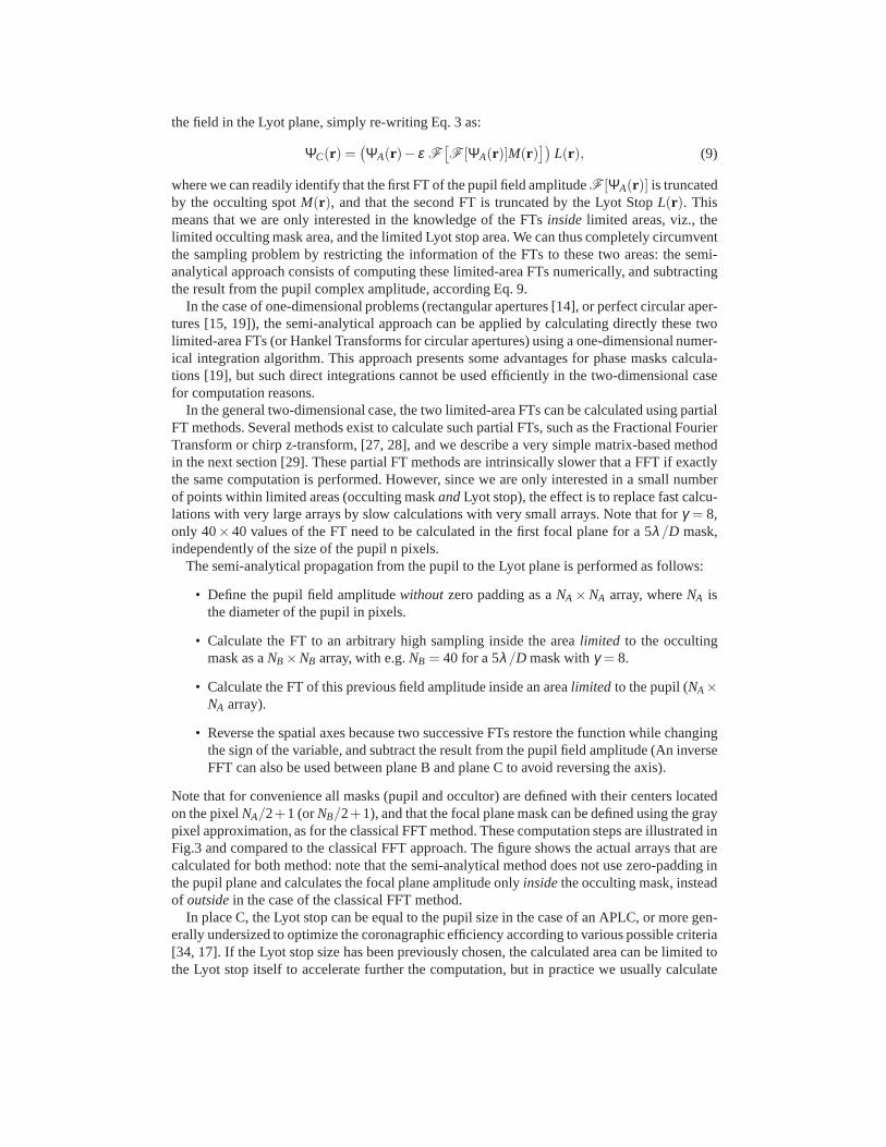
In Fig.4, Fig.5, and Fig.6, we illustrate the gain between the semi-analytical and FFT meth-ods, using the ratio of their computation costs given in Eq.18 and Eq.20. We first give some

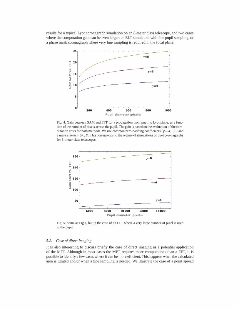
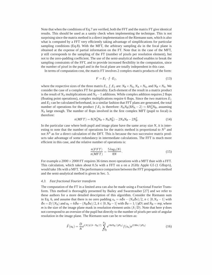
results for a typical Lyot coronagraph simulation on an 8-meter class telescope, and two caseswhere the computation gain can be even larger: an ELT simulation with fine pupil sampling, ora phase mask coronagraph where very fine sampling is requiredin the focal plane.

g 4

g 6

g 8

200 400 600 800 10000

5

10

15

20

25

Pupil diameter pixels

Gain

SAM

vs.

FFT

Fig. 4. Gain between SAM and FFT for a propagation from pupil to Lyot plane, as a func-tion of the number of pixels across the pupil. The gain is based on the evaluation of the com-putation costs for both methods. We use common zero-paddingcoefficients(γ = 4,6,8) anda mask sizem = 5λ/D. This corresponds to the regime of simulations of Lyot coronagraphsfor 8-meter class telescopes.

g 4

g 6

g 8

6000 8000 10000 12000 14000

80

100

120

140

160


Gain

SAM

vs.

FFT

Fig. 5. Same as Fig.4, but in the case of an ELT where a very large number of pixel is usedin the pupil.

5.2. Case of direct imaging

It is also interesting to discuss briefly the case of direct imaging as a potential applicationof the MFT. Although in most cases the MFT requires more computations than a FFT, it ispossible to identify a few cases where it can be more efficient. This happens when the calculatedarea is limited and/or when a fine sampling is needed. We illustrate the case of a point spread

100 200 300 400 500

240

260

280

300

320


Gain

SAM

vs.

FFT g 20

Fig. 6. Same as Fig.4, but for a Roddier or Dual Zone coronagraph with a mask size ofm =λ/D and an oversizingγ = 20. This corresponds to a maximum FFT size of 10000×10000for the 500 pixel pupil.

function (PSF) calculation with a field of view ( FOV) of 50 resolution elements in Fig.7.In this case, both techniques have similar costs with a slight advantage for one or the otherdepending on pupil size and sampling parameterγ. If the PSF is only calculated to a FOV of20 resolution elements, the MFT provides a gain by a factor ofseveral over the FFT (Fig.8). Insome applications where only the center of the PSF is needed,gains comparable to that of thecoronagraphic cases can be obtained.

g 4

g 6

g 8

g 10

200 400 600 800 1000

0.5

1.0

1.5

2.0


Gain

MFT

vs.

FFT

Fig. 7. Non-coronagraphic, direct imaging with FFT and MFT where the PSF is calculatedto a field of view of 50 resolution element (25 in radius). BothMFT and FFT have similarcosts with a slight advantage to MFTs when higher sampling isused.

g 4

g 6

g 8

g 10

200 400 600 800 10001

2

3

4

5

6

7


Gain

MFT

vs.

FFT

Fig. 8. Non-coronagraphic, direct imaging with FFT and MFT where the PSF is calculatedto a field of view of 20 resolution element (10 in radius). For alimited field of view, theMFT can be significantly faster than the FFT. This can be interesting for coronagraphic andextreme adaptive optics simulations.

5.3. Practical applications and implementation

In this section we discuss the actual performance of the semi-analytical method for a specifichardware, a 2003 Apple G5 dual processor 2Ghz computer with 4Gb RAM. We measured theperformance of this machine using the package FFTW (version3) [31] and report the results inFig.9. We considered the case of double precision complex 2Darrays, which is appropriate forcoronagraphic simulations. These results are consistent with those given on the FFTW website,but we extend them up to 8192×8192 FFT to verify that the speed does not depend stronglyon the array size. The calculations have been made with the option FFTW_PATIENT, whichoptimizes the FFT plan prior to the calculation of the FFT itself. We used single-threaded FFTsalthough the FFTW packages provides the possibility of multi-threaded calculations for furtherspeed improvement on multi-core machines.

In order to evaluate the machine’s performance for the MFT, we considered the geekbenchbenchmark software [36] which reports 1.4 Gflop/s for single-threaded dot products and 2.6Gflop/s for multi-threaded ones. It seems that dot products are slightly more efficient than theFFTW on this hardware (1.4 Gflop/s vs. 1 Gflop/s). This may be due to the easier implemen-tation of the dot-product which takes direct advantage of the processor’s vector engine. Aninteresting aspect of the MFT is that it can take advantage ofrecent multi-core computers, witheasy and efficient multi-threading of linear algebra calculations.

High level languages such at Mathematica or Matlab are well optimized for vector computa-tions. For example, we obtain 2.5 Gflop/s with Mathematica for multi-threaded dot-products ondouble precision complex arrays of sizes between 1000×1000 and 10000×10000. This resultis consistent with the benchmark results this machine (2.6 Gflop/s). In the case of a propagationfrom pupil to Lyot plane, the speed goes down to 1Gflop/s with Mathematica because the otheroperations involved in the semi-analytical method are not fully optimized with this language.

In Table 1, we compare the two methods for three pupil sizes (256×256, 512×512, 1024×1024).NA andNB are the number of pixels used in the calculation, in the pupiland focal planes.We use the same number of pixels in the Lyot plane as in the pupil. We show the effect of thesampling improvement fromλ/4D to λ/8D, obtained by zero-padding the pupil with FFTs.

0 2000 4000 6000 80000

200

400

600

800

1000

1200

1400

Array size NxN

FFTW

3onG52GHz

Mflops

Fig. 9. Normalized speed expressed in Mflop/s using the FFTW3package [31] on a 2Ghzdual-processor 2003 Apple G5 with 4Gb RAM. The normalized speed is defined as thenumber of operations divided by the execution time: 10N2 Log2(N)/T whereT is the timefor one FFT (single-threaded, double precision complex arrays). The red dots correspondto power of twos arrays.This hardware delivers approximately 1Gflop/s over the range ofarray sizes, which translates for example into 2.3s for 4096×4096 transforms, and 10s for8192×8192 transforms.

Note that for the semi-analytical method, the number of pixels NA corresponds to the pupil sizeitself, and thatNB corresponds to the focal plane mask size. For the FFT,NA corresponds to thezero-padded pupil. The timings given in the table correspond to the time for 2 FFTs calculatedwith FFTW3, neglecting the application of the focal plane mask and zero-padding time. For thesemi-analytical method, we give timings obtained with Mathematica as example.

Coronagraphic simulations are usually performed with aλ/6D to λ/8D sampling, in orderto keep the FFTs manageable. With the semi-analytical method, we can increase the precisionsignificantly, and we typically use aλ/10D or λ/20D sampling for the focal plane mask,including gray pixel approximation. This corresponds to a 40∼ 50 or 80∼ 100 pixel diametermask for a 4∼ 5 resolution element mask.

The semi-analytical method offers a total flexibility in terms of sampling in both planes, andthere is no particular limitation to the type of calculations. We present a few examples in Table2, which would hardly be achieved with FFT propagations. Forexample, one can choose toincrease the sampling in the pupil, with a modestλ/8D sampling in the focal plane, in orderto study the effect of segmentation of an ELT. We show an example of a 6000× 6000 pupilarray. This corresponds to calculations that are typicallymade on very large computer clustersusing the classical method. This would correspond to 36000×36000 FFTs withγ = 6. It isalso possible to oversample dramatically the occulting mask. This can be used to study theeffect of the actual mask shape, such as ellipticity, edge roughness, fine alignment, or effects ofatmospheric differential refraction. We give an extreme example with 1000 pixels in the pupiland a resolution ofλ/200D. This calculation would corresponds to 200000×200000 FFTs.

Another application is the simulation of Roddier or Dual Zone phase masks (DZPM), wherethe masks have a typical size ofλ/D, making the sampling problem even more critical forFFTs. The optimization of DZPM [19], which was obtained using the semi-analytical approachby integrating directly the Hankel transforms, can be studied by direct numerical simulationswith our method.

Table 1. Performance comparison of FFT-based and semi-analytical methods (SAM).NAis the number of pixels across the pupil diameter, andNB is the size of the array in thefocal plane. The FFT timings correspond to 2 FFTs calculatedwith FFTW3, and the SAMtimings correspond to an actual propagation from pupil to Lyot plane, with Mathematica.

Method Pupil Plane Image Plane TimeNA Array size Sampling Array size(NB)

FFT 256 1024 λ/4D 1024 0.22 sFFT 256 2048 λ/8D 2048 1.0 sSAM 256 256 λ/8D 40 0.06 s



Table 2. Performance of semi-analytical simulations for double precision complex arrays,with their possible applications. These calculations cannot be performed using the FFTmethod on commercial workstations, as they would correspond respectively to 200000×200000, 25600×25600, and 48000×48000 FFTs.

Method Pupil Plane Image Plane Time ApplicationNA Array size Sampling NB

SAM 1000 1000 λ/200D 1000 13.5 s Mask TolerancingSAM 3200 3200 λ/8D 40 6.1 s 4 pixel/spider on GeminiSAM 6000 6000 λ/8D 40 22 s 5 mm/pixel for 30 m ELT

6. Conclusion

In this paper we introduced a semi-analytical method to calculate the numerical propagationthrough a Lyot-style coronagraph, without any additional approximation. We showed that FFTsare not appropriate for Lyot coronagraphy because of fundamental sampling limitation, andshould be avoided for these calculations. The semi-analytical method is derived straightfor-wardly from the analysis of the wave propagation, and requires the use of a Fourier transformmethod producing arbitrary sampling in a limited area. Several methods exist to perform suchtransforms, and we suggest a matrix-based Fourier propagator that can be implemented straight-forwardly and efficiently in any language.

For coronagraphic studies for ExAO on ELTs and eight meter class telescopes, the typicalspeed improvement based on computation costs is of at least afactor twenty to fifty compared tothe classical FFT coronagraphic propagation method. In addition to speed, our semi-analyticalmethod is particularly efficient in terms of memory, as it does not involve any zero padding,and typical memory improvement is of a factor fifty. In the case of a full propagation frompupil to final focal plane, if the final FT is performed using a FFT, the semi-analytical methodis approximately three times faster than a FFT-based propagation, since the propagation time isentirely dominated by the final FT. If a reduced field of view iscalculated in the final image,

which is often the case in extreme adaptive optics coronagraphy, an MFT can be used in lieu ofan FFT. For example a factor of 5 can be gained on the last FT forNA = 400 andγ = 10, andthe overall gain with the semi-analytical method is a factorof 15.

The semi-analytical method brings a total flexibility in terms of sampling, since the samplingin the pupil and focal plane are totally independent. This enables calculations hitherto impos-sible, or requiring access to large and expensive computersclusters. For example the study offine occulting mask features and alignment, or fine pupil structures like segmentation, is nowachievable on a good laptop or on any commercial workstation.

The method may find interesting applications where a FT has tobe calculated in a limitedarea. Applications may be found in adaptive optics for anti-aliasing spatial filters, pyramidwavefront sensing, etc.

Our method also enables fast computation of optimal apodizer for APLCs, which involvesan iterative algorithm and makes computing efficiency even more critical. APLCs are one ofthe most promising concepts for high contrast imaging instruments on ELTs, and their studyrequires the optimization of the mask size according to various criteria and for broadband light.This means that a theoretical apodizer has to be calculated for each mask size in the optimiza-tion study [17]. A complete exploration of the parameter space, including effects of segmen-tation and spiders on the coronagraph is now made possible with acceptable computing times.Our method could be utilized in several current efforts focussed on ground and spaced basedcoronagraphy.

Acknowledgements

RS acknowledges partial support by a Michelson Postdoctoral Fellowship, under contract tothe Jet Propulsion Laboratory (JPL) funded by NASA. JPL is managed for NASA by the Cal-ifornia Institute of Technology and by a AMNH Kalbfleisch Fellowship. This work has alsobeen partially supported by the National Science Foundation Science and Technology Centerfor Adaptive Optics, managed by the University of California at Santa Cruz under cooperativeagreement AST 98-76783. The authors thank Lisa Poyneer, JimFienup for interesting discus-sions and Russell Makidon for helpful comments.

Fast computation of Lyot-style coronagraph...

Documents

Transcript of Fast computation of Lyot-style coronagraph...