Fast Compaction Algorithms for NoSQL Databases

Fast Compaction Algorithms for NoSQL Databases

Mainak Ghosh1 and Indranil Gupta1 and Shalmoli Gupta1 andNirman Kumar2

1University of Illinois, Urbana-Champaign

2University of California, Santa-Barbara

July 2, 2015

Big Data is Everywhere

Big Data is Everywhere

Systems experts have to cope with Big Data

Online shopping, content management, finance, education

Big Data, NoSQL and Compaction

BIG DATA

NoSQL DB

Write Performance Read PerformanceCOMPACTION

Big Data, NoSQL and Compaction

BIG DATA

NoSQL DB

Write Performance Read PerformanceCOMPACTION

We provide algorithms with provableguarantees for compaction

Results and Recommendation

Use algorithm : BalancedTree with Smallest Input

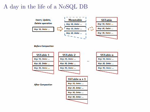
A day in the life of a NoSQL DB

Outline

I Compaction - the problem

I Compaction - our approach

I Greedy algorithms for Compaction

I Experimental results

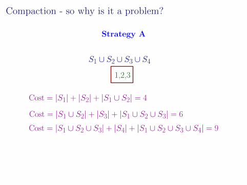
Compaction - so why is it a problem?

Strategy A

1 2 3 1,2,3

S1 S2 S3 S4


Strategy A

3 1,2,31,2

S1 ∪ S2 S3 S4

Cost = |S1| + |S2| + |S1 ∪ S2| = 4


Strategy A

1,2,31,2,3

Cost = |S1| + |S2| + |S1 ∪ S2| = 4

Cost = |S1 ∪ S2| + |S3| + |S1 ∪ S2 ∪ S3| = 6

S1 ∪ S2 ∪ S3 S4


Strategy A

1,2,3

Cost = |S1| + |S2| + |S1 ∪ S2| = 4

Cost = |S1 ∪ S2| + |S3| + |S1 ∪ S2 ∪ S3| = 6

S1 ∪ S2 ∪ S3 ∪ S4

Cost = |S1 ∪ S2 ∪ S3| + |S4| + |S1 ∪ S2 ∪ S3 ∪ S4| = 9


OR ...


Strategy B

1 2 3 1,2,3

S1 S2 S3 S4


Strategy B

2 1,2,31

S1 S2 S3 ∪ S4

Cost = |S3| + |S4| + |S3 ∪ S4| = 7


Strategy B

1,2,31

Cost = |S3| + |S4| + |S3 ∪ S4| = 7

Cost = |S2| + |S3 ∪ S4| + |S2 ∪ S3 ∪ S4| = 7

S1 S2 ∪ S3 ∪ S4


Strategy B

1,2,3

Cost = |S3| + |S4| + |S3 ∪ S4| = 7

Cost = |S2| + |S3 ∪ S4| + |S2 ∪ S3 ∪ S4| = 7

S1 ∪ S2 ∪ S3 ∪ S4

Cost = |S1| + |S2 ∪ S3 ∪ S4| + |S1 ∪ S2 ∪ S3 ∪ S4| = 7


Which choice is better?

Current approaches to Compaction

I Merge sstables when their number exceeds athreshold

I Bigtable, Cassandra, Riak


I Merge sstables when their number exceeds athreshold

I Bigtable, Cassandra, Riak

I Merge at every Insert, Update, DeleteI Optimizes for readsI Cassandra, Riak


I Merge sstables of equal sizeI Cassandra, Bigtable


I Merge sstables of equal sizeI Cassandra, Bigtable

I Prioritize more recent dataI Logs

Outline





Goals and methods

Theoretical analysis ofcompaction

Goals and methods

Theoretical analysis ofcompaction

Formulate as an optimization problem

Study algorithms and their complexity

Theoretical analysis - why?

I Theoretical analysis will provide new insights



I Better idea about limits of optimization



I Better idea about limits of optimization

I Past work: Mathieu et. al.I Merge prefix of sets - what prefix?I Cost function additive

Compaction as an optimization problem

Given sets S1, . . . , Sn, mergethem to produce a single

set


A merge is replacing somesets with their union


How many sets k?


Cost =

Read︷︸︸︷|Si1|+ . . . + |Sik|+

Write︷︸︸︷|Si1 ∪ . . . ∪ Sik|


How to do the merge sothat overall cost is

minimized?


How to select the sets ateach merge?

The tree view

S1 S2 S3 S4

S1 ∪ S2 S3 ∪ S4

S1 ∪ S2 ∪ S3 ∪ S4

Trees as blueprints formerging algorithms

The tree view

S1 S2 S3 S4

S1 ∪ S2

S1 ∪ S2 ∪ S3

S1 ∪ S2 ∪ S3 ∪ S4

Choice in the merge tree

The tree view

S1 S3 S2 S4

S1 ∪ S3 S2 ∪ S4

S1 ∪ S2 ∪ S3 ∪ S4

Choice in the ordering ofsets on leaves

Hardness result

The compaction problem isNP-hard

Proof in the paper

Hardness result

View - find the tree and the ordering

Hardness result

Fixed tree - choice on ordering. Is this NPhard?

Hardness result

Yes. For some trees we prove NP hardness

Hardness result

Compaction reduces to this problem

Outline



I Greedy algorithms forCompaction


Greedy strategies

Maintain a collection :S1, . . . , Sn

Greedy strategies

We always merge 2 sets at atime

Greedy strategies

Strategy determines whichtwo we merge

Greedy strategies

We have n− 1 merge stepsin all

Greedy strategies

Main intuition : Merge sothat larger sets form later

Greedy strategies

Smallest Output (SO)

Minimize |Si ∪ Sj|

Greedy strategies

Smallest Input (SI)

Choose two smallest sets

Greedy strategies

Balanced Tree (BT)

Ensure a balanced merge tree

Greedy strategies

Largest Match (LM)

Maximize |Si ∩ Sj|

Greedy strategies

Balanced Tree, SmallestInput (BT(I))

Combine Balanced Tree withSmallest Input

Approximation guarantee

SI, SO, BT are all O(log n) approximations

Approximation guarantee

BT is Ω(log n) in worst case

Outline





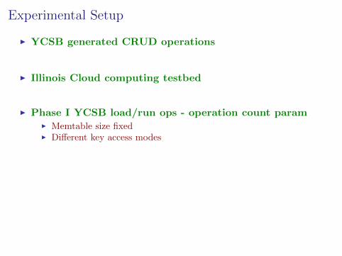
Experimental Setup

I YCSB generated CRUD operations

Experimental Setup


I Illinois Cloud computing testbed

Experimental Setup



I Phase I YCSB load/run ops - operation count paramI Memtable size fixedI Different key access modes

Experimental Setup




I Merge sstables in Phase II

Experimental Setup




I Merge sstables in Phase II

I Hyperloglog to estimate set sizes with SO (Flajolet et.al.)

Experimental results

0 20 40 60 80 1000

10K

20K

30K

40K

50K

Update Percentage

Tim

e(m

s)

BT(I)

RANDOM

BT(I) is the most efficient in implementation


Update Percentage

Cost/10

6

0 20 40 60 80 100

0.2

0.6

1.0

1.4

1.8

BT(I)

RANDOM

BT(I) is the best cost wise


5000

20000

35000

50000

3× 106 6× 106 9× 106

Cost

Tim

e(m

s)

SI performance

True cost is modeled accurately by our costfunction


Memtable size

10 100 1000 10000100

1000

104

105

106

107

Cost Lower Bound

BT(I)

Logscale const. difference

Performance within constant factor

Open Questions

SO, SI are better thanO(log n) - proof?

Finale

Use algorithm : BalancedTree with Smallest Input

Fast Compaction Algorithms for NoSQL Databases

Documents

Transcript of Fast Compaction Algorithms for NoSQL Databases