Fast and Reliable Example-Based Mesh IK for Stylized Deformations

Kevin Wampler∗

Adobe Systems Inc.

Abstract

Example-based shape deformation allows a mesh to be easily ma-nipulated or animated with simple inputs. As the user pulls parts ofthe shape, the rest of the mesh automatically changes in an intuitiveway by drawing from a set of exemplars. This provides a way forvirtual shapes or characters to be easily authored and manipulated,or for a set of drawings to be animated with simple inputs. We de-scribe a new approach for example-based inverse kinematic meshmanipulation which generates high quality deformations for a widerange of inputs, and in particular works well even when providedstylized or “cartoony” examples. This approach is fast enough torun in real time, reliably uses the artist’s input shapes in an intu-itive way even for highly nonphysical deformations, and providesadded expressiveness by allowing the input shapes to be utilized in away which spatially varies smoothly across the resulting deformedmesh. This allows for rich and detailed deformations to be createdfrom a small set of input shapes, and gives an easy way for a set ofsketches to be brought alive with simple click-and-drag inputs.

Keywords: deformation, shape modeling, as-rigid-as-possible,shape space

Concepts: •Computing methodologies → Animation; Mesh mod-els;

1 Introduction

Even a relatively simple shape in computer graphics is typicallyrepresented by a polygonal mesh which is too complex to manuallymodify vertex by vertex, and certainly not in a real-time applica-tion. Higher level tools are instead necessary to control the shapeby manipulating a small set of parameters. Shape deformation pro-vides one convenient way of doing this. The user controls the posi-tion of a few vertices or localized areas of the mesh, and the properdistortion for rest of the shape is automatically inferred.

The user’s input while interacting with a deformable mesh can bemodeled as constraints which must be satisfied by the resultingshape – for instance specifying the position to which a particu-lar vertex must be moved. Traditionally, the deformed shape is

∗e-mail:kwampler@adobe.comPermission to make digital or hard copies of all or part of this work forpersonal or classroom use is granted without fee provided that copies are notmade or distributed for profit or commercial advantage and that copies bearthis notice and the full citation on the first page. Copyrights for componentsof this work owned by others than ACM must be honored. Abstracting withcredit is permitted. To copy otherwise, or republish, to post on servers or toredistribute to lists, requires prior specific permission and/or a fee. Requestpermissions from permissions@acm.org. c⃝ 2016 ACM.SA ’16 Technical Papers,, December 05-08, 2016, , MacaoISBN: 978-1-4503-4514-9/16/12DOI: http://dx.doi.org/10.1145/2980179.2982433

then computed as one which bends or stretches the input shape assmoothly as possible while still satisfying the specified constraints.Unfortunately both real-world and artist-designed shapes often donot deform in this manner, instead deforming in a way which ismore complex: sections will twist, thin, or balloon, muscles willbulge, specific parts will curve or bend, etc.

We consider the creation and manipulation of models capturingthese sorts of complex deformations. We focus in particular onthe interactive manipulation or animation of virtual shapes or char-acters, including highly stylized artist-created examples. To en-sure that our deformable models are easy to create, even for non-technical users, we base our approach within the paradigm ofexample-based deformations where multiple shapes are providedas input and the range of features observed in these shapes is usedto inform the resulting deformation. This has the advantage that itcan be applied directly to free form meshes without any need forcomplicated character rigs or manually crafted parameterizations.

After a set of input shapes is provided, the natural question thatarises is precisely how they should be combined to create a de-formed shape based on a user’s inputs. In the context of interactiveshape manipulation or animation, this technique should be both fastenough to run in real time, and reliable in that the result reflects thedesign of the inputs shapes in an intuitive and easily predictablemanner, even for highly stylized inputs. Finally, because of the ef-fort required in an artist creating a large number of input shapes, theapproach should also be expressive in that a wide range of visuallyplausible deformations can be created from a relatively small set ofinputs.

With this in mind, we propose a novel approach to example-basedshape deformation. This approach generalizes the traditional as-rigid-as-possible deformation energy to allow for example-baseddeformations, and is fast enough to run in real time. We achievereliable deformations by viewing the issue of reliability as a combi-nation of a scattered data interpolation and an elastic deformation,and deriving a new form of an example-based elastic energy com-bining properties of both. We also support the easy authoring ofexpressive models by supporting deformations that employ the pro-vided input shapes in a manner which is spatially localized and cansmoothly vary over the mesh.

Our primary contribution is the development of a technique for real-time kinematic example-based mesh deformation which achieveshigh-quality and intuitive results across a wide range of cases withno parameter tuning, including highly non-physical stylized inputs.This involves three sub-contributions working in concert:

1. We develop a new approach for generalizing a non-example-based elastic energy into an example-based elastic energywhich improves how reliably the inputs shapes are used, byconsidering not only the space spanned by the input shapes,but also the desirability of different shapes within this space.This combines the strengths of existing shape space ap-

proaches with some beneficial properties typical of scattereddata interpolation.

2. We give an example-based generalization of an as-rigid-as-possible energy as applied to a mesh parameterized with lin-ear blend skinning, as well as an associated optimization algo-rithm. This allows high-quality deformations to be calculatedin real time even for high-resolution meshes.

3. We describe an example-based elastic energy which allowsthe degree to which each input shape is used to smoothlyvary over the resulting mesh while retaining real-time perfor-mance, building upon previous approaches for plastic defor-mations [Jones et al. 2016].

2 Related Work

The ability to deform a potentially complex input shape by pro-viding a small set of user-specified constraints is an important andwell-studied problem in computer graphics, a survey of which isprovided by Botsch and Sorkine [2008]. Typically the input shape isrepresented as a triangulated mesh or tetrahedralized volume so thatcalculating the deformation amounts to computing new positionsfor the vertices in the shape. The most popular way of approachingthis problem for free form meshes is to minimize an elastic en-ergy on the shape subject to some set of user-specified constraints.This energy measures the accumulation of local distortions of thedeformed shape with respect to the input shape. Of particular rel-evance to our work is as-rigid-as-possible (ARAP) shape deforma-tion [Igarashi et al. 2005; Sorkine and Alexa 2007; Liu et al. 2008;Chao et al. 2010; Jacobson et al. 2012a; Levi and Gotsman 2015]which measures local distortions by the degree of non-rigidity theyinduce. ARAP deformations are relatively simple to formulate, effi-cient to compute, and normally give rise to visually pleasing results.

Most shape deformation approaches are formulated with respect toa single input shape, which does not allow detailed control overhow the deformation should deviate from this base shape. To rem-edy this, our method draws inspiration from an existing class oftechniques which rely on multiple input shapes. One facet of thisis the problem of shape interpolation, in which a deformed shape isgenerated by blending the input shapes with different pre-specifiedweights. In some contexts such as the use of blendshapes in faceanimation [Bergeron and Lachapelle 1985] this interpolation canbe performed directly in the space of vertex positions, but in mostcases this leads to obvious artifacts, and variety of alternatives havebeen proposed. These include using alternative parameterizationssuch as pyramid coordinates [Sheffer and Kraevoy 2004], interpo-lating along geodesics in a Riemannian space [Kilian et al. 2007],guiding the interpolation by clustering poses in a database [Gaoet al. 2013], or by explicitly considering the rigid and non-rigidcomponents of the interpolation in an as-rigid-as-possible approach[Alexa et al. 2000; Chao et al. 2010; Levi and Gotsman 2015].

Shape interpolation is sufficient if it is reasonable to explicitly spec-ify the interpolation weights, but in many situations it is desirableto infer these weights automatically. Depending on the context, thiscan be done either with a kinematic technique such as ours, or witha dynamic technique when one wishes to calculate the deformationsin the context of a physical simulation. The most common formu-lation within this latter category augments the physical dynamicalequations with a constraint that the simulated shape lie near thesubspace spanned by the input shapes [Martin et al. 2011; Koyamaet al. 2012; Schumacher et al. 2012; Song et al. 2014; Zhang et al.2015]. Jones et al. [2013] take a similar approach and constrain thesimulation to lie within a user-specified simplicial complex on theinput shapes. A related method is described by Jones et al. [2016]in the context of plastic, rather than elastic deformations.

Our approach is kinematic rather than dynamic in that it does notrely on any physical simulation and instead calculates the deformedshape purely from the input shapes and user-specified constraints.This is done in the spirit of inverse kinematics where the user pro-vides positional constraints on localized portions of the mesh. In-verse kinematic approaches are popular with kinematic skeletons,a context in which Grochow et al. [2004] use a set of exampleskeletal poses to guide the result. An analogous operation in thecontext of free form mesh deformation was introduced by Sumneret al. [2005] and later improved by Der et al. [2006] and Frohlichand Botsch [2011]. Alternatively, Lewis and Anjyo [2010] and Seoet al. [2011] perform a similar operation in the specific context offace deformation. The basic technique used by these approaches issimilar to that of example-based dynamics in that the deformationis chosen to lie as close as possible to a linear or convex subspacespanned by the example shapes.

As an alternative to choosing the deformed shape as one nearest to asubspace spanned by the input shapes, it is natural to view calculat-ing the deformation as a scattered data interpolation problem. Thatis, choose the deformed shape not based on an energy measuringthe distance from a subspace, but instead as one which blends be-tween nearby input shapes. Often this is done by parameterizing thedeformation within an abstract pose space [Lewis et al. 2000] andusing traditional scattered data interpolation techniques such as ra-dial basis functions [Sloan et al. 2001; Zhang et al. 2004] or kernelCCA [Feng et al. 2008] within this space, after which the interpo-lated shape is calculated, sometimes with explicit detail preserva-tion [Weber et al. 2007; Huang et al. 2011; Hahn et al. 2014]. Inmany cases, particularly in restricted contexts such as skeletal rigsor face deformation, these methods perform well. With respect toelastic energy-based approaches, however, they have the disadvan-tage that they require a (sometimes large) set of input shapes and arenot designed to calculate deformations when given only one or veryfew input meshes. One notable approach which combines some as-pects of elastic energy with scattered data interpolation is given byMilliez et al. [2013], who discretely choose pieces of a larger modelfrom a set of example shapes by projecting to the nearest neighboras measured by an ARAP-based distance metric.

Also related to our approach is the topic of mesh skinning [Seder-berg and Parry 1986], whereby the deformation of a shape is di-rectly parameterized by a small set of controls, with the influenceof these controls propagated to the entire mesh. Using a cage forthis parameterization is a popular approach, and a survey is givenby Nieto and Susn [2013]. In the case of character animation it maymake more sense to bind the mesh to the pose of an underlying kine-matic skeleton [Baran and Popovic 2007; Wareham and Lasenby2008]. In our implementation, the user places a set of handles atlocalized positions on the mesh, and the influence of these handlesover the mesh is computed with bounded biharmonic weights [Ja-cobson et al. 2011]. Jacobson et al. [2012b] and Wang et al. [2015]provide alternative methods for handle-based skinning.

3 Overview

The input to our mesh deformation method is a set S of exampleshapes. Each of these shapes is represented by a triangular meshand describes an example rest shape for some object. These meshesmust have the same vertex set P and the same triangle set, so theyonly differ in the positions of their vertices. The shape of the sth ex-ample mesh, denoted by ps, is represented with a one-dimensionalarray of length |P|, each element of which is a k-dimensional vec-tor describing the position of a single vertex, where k is either twoor three depending on the dimension of the space the mesh is em-bedded in. All of the ps example meshes are collected together intoa single |S| × |P| array denoted P . Recall that each element of P

is a k-dimensional vector, rather than a single scalar.

We allow a user to manipulate a mesh by controlling a set H ofhandles. Each handle is associated with a subset of the vertices ofthe mesh. A deformed mesh q is computed by the user specifyingthe position of each handle, from which the positions of the remain-ing vertices are computed automatically. For any particular settingof the desired positions of each handle in H, there is an associatedconstraint set C such that q ∈ C if and only if each handle in q islocated at its desired position.

As is standard with existing example-based mesh deformation ap-proaches, we compute a deformed mesh q by minimizing an elasticenergy E(q,P , b). Here q is an array of length |P|, each elementof which is a k-dimensional vector describing the position of a sin-gle vertex in the deformed mesh. P is an array combining the ver-tex positions of all of the ps input meshes as previously described,and b is a length-|S| array of scalars such that bs gives the degree ofcontribution for the input mesh ps to q. We will further enforce thatb is nonnegative and sums to one. In section 5 we will show how bcan be extended to allow spatially localized interpolations, but fornow will use this simplified form to make it easier to compare toprevious work.

The general form of the optimization used to solve for an example-based mesh deformation as applied to the context of mesh-basedinverse kinematics can then be written:

qopt, bopt =argminq∈C,b

E(q,P , b) (1)

The primary concern of this paper is to derive a definition for Eappropriate for fast and reliable mesh-based inverse kinematics. Itis tempting to view this problem as either a trivial generalizationof mesh interpolation, or as a trivial restriction of example-basedelastic material simulation. It is perhaps surprising then that thereare difficulties specific to mesh IK that do not appear in either ofthese two contexts. To better motivate our approach we will beginby examining these alternatives.

To provide a pedagogical example to compare the different ap-proaches, consider a simple square-shaped mesh. As the squareis stretched it should first puff outward, and then thin inward as it isstretched yet further. This behavior is specified with the three inputmeshes shown in figure 1. Each of three input shapes is shown ina different color. The deformation is controlled by specifying theposition of three handles, each of which is shown as a black dot.We will consider in particular what happens as the user drags therightmost handle.

Figure 1

Although this would intuitively appear to be a very simple exam-ple, it poses surprising difficulties for existing approaches. Broadlyspeaking these existing approaches can be divided into two cate-gories depending on how E is specified.

3.1 Motivation: Energy Interpolation

One class of existing technique defines E by interpolating betweenthe values of a non-example-based elastic energy Ed as applied to

each ps shape independently:

E(q,P , b) =

|S|∑s

bs Ed(q,ps) (2)

An energy of this form is typically applied in the context of shapeinterpolation, where b is assumed to be fixed in advance and onlyq is optimized over [Alexa et al. 2000; Chao et al. 2010; Levi andGotsman 2015]. If we instead apply an energy of this form to theproblem of mesh IK by optimizing over both q and b as prescribedby equation 1, the results exhibit a rather serious artifact, as shownin figure 2 row c. The form of equation 2 guarantees that E is al-ways minimized when b is zero except for a one at the entry of theinput shape corresponding to the minimal value of Ed(q,ps). Theresulting deformation thus discretely jumps from one shape to an-other as the user drags the handles, rather than smoothly deformingas the artist likely intended.

Energies of this sort have a natural interpretation as a scattered datainterpolant. Since the optimal value of b is always zero except forthe input shape for which Ed is minimized, it corresponds to near-est neighbor interpolation by projection to the nearest Voronoi cellusing a measure of distance as defined by Ed(q,ps). Because ofthis, despite the defect of discontinuous transitions, all of the inputshapes are reliably used.

3.2 Motivation: Shape Spaces

The second class of elastic energies used for example-based meshdeformation rely on the concept of a shape space, also sometimescalled an example manifold. As with energy interpolation this alsorelies on a non-example-based elastic energy Ed, but applies it toan interpolation of the input shapes, or of features computed fromthe input shapes. Using blend(P, b) to denote a function whichinterpolates the p1, . . . ,p|S| input meshes using b as a vector ofinterpolation weights, these energies can be expressed as:

E(q,P , b) = Ed (q, blend(P, b)) (3)

This class of approaches is sometimes used for mesh IK [Sum-ner et al. 2005; Der et al. 2006; Frohlich and Botsch 2011], buthas seen particular success when applied to example-based elasticmaterial simulation [Martin et al. 2011; Koyama et al. 2012; Schu-macher et al. 2012; Song et al. 2014; Zhang et al. 2015], where itperforms quite admirably. Since the goal for simulation is to havethe mesh deform in a physically plausible manner guided by the ex-ample shapes, the passive dynamics of the mesh act as a powerfulregularizer for the deformation. Shape spaces are a natural fit here,since within the shape space, the passive dynamics dominate. Forinverse kinematics, however, this approach also has artifacts. Thenature of the artifacts depends on whether blend(P, b) is a linear ornonlinear function.

If blend(P, b) is linear, as in the linear deformation gradients ofSumner et al. [2005], then deformation of the example in figure1 is often ambiguous, since many linear combinations of the inputshapes may all satisfy the user’s IK constraints. This is shown infigure 2 row d, where the green shape is essentially ignored and a50/50 blend of the red and blue shapes is used instead.

It is more common that blend(P, b) is nonlinear and that it com-putes a feature vector larger than the number of degrees of freedomin q. As described by Schumacher et al. [2012], this means thatE will typically be zero only when q is exactly equal to some ps.This avoids the ambiguity inherent in linear shape spaces, but addsthe complication that a nonlinear shape space may give rise to op-timization difficulties such as local minima. Examples of artifacts

Figure 2: Each row shows a different deformation method applied to the inputs in figure 1 as the rightmost handle is dragged to stretch andthen un-stretch the shape. The graphs on the left show the blending weights over time. From top to bottom: a) Our method without rotations,b) Our method with rotations, c) energy interpolation [Chao et al. 2010], d) linear shape space (our method with λ = 0), e) nonlinear shapespace [Schumacher et al. 2012].

resulting from this are shown in figure 2 row e, which exhibits bothdiscontinuous jumps as a new local minimum arises or disappearsand the optimization converging to a suboptimal local minimumwhen the box is contracted, using a blend of the red and blue shapeswhen the green shape would lead to a lower error.

4 Interpolation Energy

At the core of our method is an elastic energy which, when min-imized subject to some inverse kinematic constraints, interpolatesefficiently and reliably between a set of example meshes, even forhighly stylized and exaggerated deformations. Although our elas-tic energy is based on an as-rigid-as-possible (ARAP) energy, wewill consider it first in a simplified form. This will make it easierto compare against the alternative energies described in section 3without the additional complications introduced by the full ARAP-based formulation.

As with previous approaches such as energy interpolation (sec-tion 3.1) and shape space energies (section 3.2), we constructan example-based elastic energy E(q,P, b) by modifying a non-example-based energy Ed(q,p). Here, q, P, p, and b take thesame meanings as previously introduced in section 3. At runtime,the vertex positions in the deformed mesh q are generated by min-imizing E subject to some user-specified constraints enforcing thatq ∈ C where C represents the subset of deformations in which thehandles are correctly located at their user-specified positions.

A primary function of the elastic energy E is used to interpolatebetween the artist-provided input shapes as the user-specified con-straint set C changes (i.e. as the user clicks and drags the handles).Given this, it is useful to consider what properties E should satisfynot only as an elastic energy, but also what properties its minimiza-tion has as a method for scattered data interpolation.

Firstly, E should satisfy some basic properties which define it as anexample-based energy. Both energy interpolation and shape spaceenergies already satisfy these:

1. If bs = 0, then E(q,P, b) is independent of ps.

2. When b is entirely zero except for bs = 1, then E(q,P, b) =Ed(q,ps). As a consequence, E reduces to Ed when there isonly one example mesh.

3. E should inherit any symmetries of Ed. For example, if Ed isinvariant to rigid transformations, then E should be too.

Next, from the perspective of scattered data interpolation there aresome properties that E should satisfy in how the contribution ofeach of the input shapes relates to the constraint set C. There are twoclasses of artifacts that need to be avoided. Firstly small changes inthe handle positions should not lead to discontinuous changes inthe result, as in figure 2 row c. Secondly, we want to ensure thatinterpolations of similar shapes are preferred over interpolations ofdisparate shapes, avoiding the artifact in figure 2 row d where thegreen shape is ignored in favor of a blend of the red and blue shapes.

4. In practice, the vector qopt = argminq∈C,b E(q,P, b)

should vary C0 continuously with respect to C.

5. Given some deformed mesh q and defining bopt =argminb E(q,P, b), then bopt should typically be zero at en-tries corresponding to input shapes which are dissimilar fromq. Relatedly, minb E(q,P, b) should be zero if and only ifq = ps for some s (up to the symmetries of E).

Finally, although it is not possible to entirely eliminate local min-ima since they are present even in a standard non-example-basedARAP energy, we wish to mitigate their effects. We formulate thisby ensuring that:

6. If Ed is convex, then so is E.

This last point has a small subtlety which is worth noting. We re-quire not only that a convex Ed leads to a convex E, but also that Edoes not depend on the nonconvexity or nonlinearity of Ed in orderto satisfy properties 1-5. This is in contrast to shape space energieswhich, as illustrated in figure 2 rows d and e, give either a convexoptimization (row d) or prefer interpolating between similar inputshapes (row e), but not both.

To our knowledge no existing elastic energy satisfies all of theseproperties. For example although most techniques for example-based mesh deformation satisfy properties 1-3, energy interpolationfails to satisfy property 4, shape space energies with a linear blendfunction fail to satisfy property 5, and shape space energies with anonlinear blend function fail to satisfy property 6. Each of theseleads to noticeable artifacts when applied to stylized mesh-basedinverse kinematics, as shown in figure 2 rows c-e.

Our technique provides example-based deformations satisfying theabove six properties by employing a novel method for generalizinga non-example-based energy Ed(q,p) to an example-based energyE(q,P, b). At its core, this approach is quite simple, and begins

by calculating a set of |S| scalar constants d1, . . . , d|S| as:

ds = minqs∈C

Ed(qs,ps) (4)

Here qs is used instead of q to indicate that a deformed mesh iscomputed independently for each ds. The different ds values arecollected together into a single length-|S| vector d. Our example-based elastic energy E is then defined as.

E(q,P, b) = Ed(q, blend(P, b)) + λdT b

The optimization to solve for q can then be simply defined as:

argminq∈C,b

Ed(q, blend(P, b)) + λdT b (5)

s.t.|S|∑s

bs = 1

0 ≤ bs 1 ≤ s ≤ |S|

where λ is a pre-specified scalar (set to 0.5 unless otherwise noted).Note that the value of each ds only depends on ps and C so in prac-tice they need only be recomputed once each time the user movesa handle. We also note that the simple formulation shown herewill be complicated somewhat later on when we integrate it with anARAP energy, particularly by the allowance that the bs values mayspatially very over the mesh, but the core intuition behind it willremain the same.

This optimization can be interpreted in several different ways.Firstly it can be viewed as a weighted-L1 regularization applied tothe shape space distance Ed(q, blend(P, b)), where the weights inthe regularization are themselves defined by minimizing Ed. Thishas the effect of penalizing the example meshes for which ps is farfrom C, as defined by Ed. The particular weights in d are impor-tant to the correct functioning of our energy. For example, usingan unweighted L1 regularizer on b has no effect, since the con-straint that b be nonnegative and sum to one already enforces that∥b∥1 = 1, so the regularizer only adds a constant term and doesnot alter the location of the optimum. Alternatively equation 5 canbe viewed as taking an energy interpolation formulation and usinga distance-from-subspace term Ed(q, blend(P, b)) to smooth outthe discontinuous transitions. We prefer to interpret it as a kind ofhybrid between energy interpolation and shape spaces, and indeedit is equivalent to a shape-space energy when λ = 0 and approachesenergy interpolation as λ → ∞.

When applied to example-based mesh deformation, we find thatthe value of λ = 0.5 works well. Larger values of λ increasinglytend toward abrupt transitions between the input shapes. Smaller(but non-zero) values instead tend toward a generalized version ofpiecewise linear interpolation, with the drawback that the influenceof an input shape can fall off increasingly abruptly when the de-formation moves outside the convex span of the input shapes. Seefigure 8 for examples of these behaviors. We prefer defining Ed us-ing the distance ∥q−p∥2 instead of the squared distance ∥q−p∥22since within span of the input shapes the non-squared version betterapproximates a piecewise linear interpolation for non-infinitesimalvalues of λ. We should also note that this method only satisfies thecontinuity property (number 4 in the list at the beginning of this sec-tion) when Ed is strictly convex, so using a non-squared distancefor Ed does not necessarily reconstruct f as an everywhere contin-uous function. Although this is possible to fix by redefining Ed tobe strictly convex (or, in our case, strictly convex when holding aset of local rotations fixed), we have observed that the discontinu-ities are rare enough that they do not visually impact the quality ofthe results.

5 As Multi-Rigid as Possible Deformations

We use the approach described in section 4 to derive a new tech-nique for example based mesh manipulation based on an as-rigid-as-possible elastic energy. We call this technique as-multi-rigid-as-possible (AMRAP) mesh deformation. Since this approach is basedon the optimization in equation 5, it inherits many of the desirableproperties of as-rigid-as-possible deformations, such as invarianceto rigid transformations and minimization of scale and shear dis-tortions as well as the ability to robustly and smoothly interpolatebetween the input shapes. In addition, this approach also supportsspatially localized changes in how the different example shapes arecombined. To allow real-time interaction even with high-resolutionmeshes, we employ a reduced coordinate model based on linearblend skinning, described next.

5.1 Deformation Model

As noted in section 3, we allow a user to manipulate a mesh bycontrolling a set H of handles. We employ a linear blend skinningmodel where each handle is associated with a per-shape k×(k+1)-dimensional matrix representing an affine transform for the handle.These transforms are packed into a |H| × |S| array T so that theaffine transform for the hth handle and sth shape is Ths. The positionof the complete set of vertices in P describing a deformed mesh iscomputed from T by linear blend skinning. This uses a |H| ×|P| matrix of skinning weights W where Whp gives the amount ofinfluence that the hth handle has on the position of the pth point.These skinning weights can be defined in many ways, includingpainting by an artist, but in our implementation we select a subset ofthe vertices in the mesh for each handle, fix their skinning weightsto 1, and extend the weights to the rest of the mesh using boundedbiharmonic weights [Jacobson et al. 2011]. The length-|P| array ofk-dimensional points q giving the shape of the deformed mesh isthen computed as:

qp =∑hs

WhpThs

[P sp

1

]=∑hs

MhspTThs (6)

where to reduce notational clutter the bounds of the sum (i.e. h =1 . . . |H|, s = 1 . . . |S|) are taken to be implicit from the names ofthe indices it is summing over. M is a |H| × |S| × |P| array oflength-k+1 row vectors combining the effect of W and P on q interms of T.

Although this deformation model is mathematically equivalent tostandard linear blend skinning, its interpretation is slightly differ-ent since it combines both different handles and different shapes.For instance, scaling a particular Ths by a constant factor increasesor decreases the contribution of the sth shape to q in the vicinityof the hth handle. On the other hand, multiplying each Ths by thesame rigid transformation for 1 ≤ s ≤ |S| has the effect of rigidlytransforming the portion of q near the hth handle. Equation 6 thusdescribes q as a combination of spatially localized geometric trans-formations and interpolations of the input meshes.

This deformation differs from that described by Jones et al. [2016]in that it is entirely linear. This simplifies its use in the AMRAPoptimization and is helpful in allowing our method to run in realtime. Although this linear nature means that it is capable of rep-resenting highly distorted deformations, the fact that the AMRAPenergy attempts to preserve local rigidity naturally avoids these sit-

uations and we have not observed any artifacts resulting from thislinearity in practice.

5.2 Deformation Energy

Describing the shape of a deformed mesh by manually specifyingT is tedious, particularly so when there is more than one shape. Weinstead allow a user to directly manipulate the shape with a simpleclick-and-drag interface and automatically infer T via an energyminimizing optimization. This leads to both automatic geometricdistortions and automatic determination of how much each of theinput shapes contributes to different regions of the final mesh.

Our deformation energy is based on generalizing an as-rigid-as-possible (ARAP) energy [Igarashi et al. 2005] with equation 5 toallow interpolation between a set of shapes. This leads to an as-multi-rigid-as-possible energy where the rigidity is measured withrespect to the set of input shapes described by p1, . . . ,p|S| ratherthan with respect to a single mesh.

A standard ARAP energy, denoted Earap, measures the distortionof a shape q with respect to a reference shape p by a sum of localdeviations from perfect rigidity. We represent both q and p as anarray of size |P|, each element of which is a k-dimensional vectorrepresenting the position of a single vertex. Restated here for refer-ence in the form given by [Jacobson et al. 2012a], this energy canbe written:

Earap=1

2

∑g

∑(p1,p2)∈Gg

cgp1p2

∥∥(qp2−qp1

)−Rg

(pp2

−pp1

)∥∥2

=1

2

∑g

∑e∈Gg

cge

∥∥∥∥∥∑p

Aepqp−Rg

∑p

Aeppp

∥∥∥∥∥2

=1

2

∑g

Eg(q,Rg,p) (7)

Where G is a set of edge groups and g indexes over 1, . . . , |G|.As in equation 6, the bounds of the summation are taken to be im-plicit from the names of the indices being summed over. Further,Rg ∈ SO(k) is a local rotation matrix associated with the gth edgegroup, cge is a weighting term typically calculated with the cotan-gent Laplacian [Chao et al. 2010], and A is the |E| × |P| (sparse)directed adjacency matrix corresponding to the set E of edges ofthe triangular mesh on q. As suggested by [Jacobson et al. 2012a]we compute G by performing k-means clustering on W with thenumber of clusters set to 2|H|. This allows us to use a relativelysmall number of edge groups and is important for real-time perfor-mance since the support for spatially localized blending includesadditional variables and constraints for each edge group (equation20).

Our AMRAP energy is based on generalizing equation 7 to interpo-late between multiple shapes using the format outlined previouslyin section 4. Doing so is slightly more involved than equation 5would make it appear for two reasons. Firstly we must modify theblend function to account for the fact that an ARAP energy explic-itly optimizes over a local rotation matrix for each edge group inG. Secondly, the blend function will need to be further modified inorder to support interpolations which spatially vary over the mesh.

Both these modifications are achieved by defining the local rotationmatrices and the blend weights both per shape and per edge group.Accordingly, we represent the collection R of all the local rotationswith a |G| × |S| array of k × k rotation matrices. Similarly, theper-edge-group blend weights for the different p1, . . . ,p|S| shapesin P are collected into a |G| × |S| matrix denoted B. The interpo-lation function used to define the analogue of a shape space for an

AMRAP energy is then defined as:

[blendg(P , B)]e =∑sp

BgsRgsAepP sp (8)

To avoid scaling artifacts or negative shape contributions we alsoconstrain ∀g, s : Bgs ≥ 0 and ∀g :

∑s Bgs = 1. Since

blendg(P , B) computes a vector of interpolated edge lengths, weuse the notation [blendg(P , B)]e to refer a single element corre-sponding to the eth edge.

This function can be interpreted as, for the gth edge group and eachedge e ∈ Gg first rotating the corresponding edge for each shape inS by Rgs, then linearly blending the edges for the different shapestogether according to the weights given by Bgs. Because the in-stances of an edge group within each shape are rotationally aligned,and because each edge group relates only to a small localized por-tion of the complete mesh we avoid the normal artifacts associatedwith linearly interpolating directly between vertex positions.

Given the definition of the blend function in equation 8, the elasticenergy Ed on which the AMRAP energy is based is analogous to astandard ARAP energy, but employing the blend function to locallyinterpolate and rotate the different input shapes:

Ed(q,B,R,P )=1

2

∑g

∑e∈Gg

cge

∥∥∥∥∥∑p

Aepqp−blendg(P ,B)e

∥∥∥∥∥2

(9)

We also require a definition for d in equation 5. To support spa-tially varying geometric deformations within an ARAP-style for-mulation, we extend this somewhat by instead computing a |G|×|S|matrix D. Each column of this matrix is defined by first solv-ing qs = argminq∈C,R Earap(q,R,ps) then extracting the per-edge-group costs by setting Dgs = Eg(qs,R,ps). The functionEarap (from equation 7) appears instead of Ed since when ap-plied to just a single shape ps, Ed(q, B,R,ps) reduces exactlyto Earap(q,R,ps).

Finally, the full AMRAP elastic energy is written in a form analo-gous to that prescribed by equation 5.:

E(q, B,R,P ) =√

Ed(q, B,R,P ) + λ∑gs

Bgs

√Dgs (10)

The use of the square root in the definition allows for the results tobetter approximate piecewise linear interpolations as C is changed.The version without the square roots also works relatively well, andmay be a suitable alternative in situations where a low computa-tional cost is paramount. Nevertheless, since we have found thatversion in equation 10 can be computed quickly enough in our testcases, we use it for all of the examples in this paper.

5.3 Solving with Rotations Held Fixed

We solve for a deformed mesh by minimizing equation 10 withan alternating algorithm similar to that used for a standard ARAPenergy. This algorithm alternates between two steps. First R is heldfixed and T and B are solved for. Then in the second step T andB are held fixed and R is solved for. This process is repeated untilconvergence, or until a new frame needs to be displayed in whichcase it is terminated early. We begin by discussing how to solve forT and B under the assumption that R is held constant.

Since we use the linear blend skinning deformation model givenin section 5.1, solving for T is equivalent to solving for the vectorof vertex positions q representing the deformed mesh. Plugging

equation 6 into equation 9 to express Ed(q, B,R,P ) in terms ofT as Ed(T, B,R,P ) and expanding yields Ed as the sum of threeterms:

Ed(T, B,R,P ) (11)

=1

2Ed1(T,P )− Ed2(T, B,R,P ) +

1

2Ed3(B,R,P )

The terms in this equation are straightforward to calculate and toimplement in code, if somewhat notationally awkward to express:

Ed1(T,P ) =∑

h1h2s1s2

tr(Th1s1 Lh1h2s1s2T

Th2s2

)(12)

with

Lh1h2s1s2 =∑p1p2

Lp1p2Mh1s1p1MTh2s2p2

(13)

Lp1p2 =∑g

∑e∈Gg

cgeAep1Aep2 (14)

Where L is a |P| × |P| matrix and L is a |H| × |H| × |S| × |S|array of (k + 1)× (k + 1) matrices.

Similarly, Ed2 is expressed as:

Ed2(T, B,R,P ) =∑

ghs1s2

Bgs1 tr(Rgs1Kghs1s2T

Ths2

)(15)

with

Kghs1s2 =∑p

Kgs1pMThs2p (16)

Kgsp1 =∑p2

∑e∈Gg

cgeAep1Aep2P sp2 (17)

Where K is a |G| × |S| × |P| array of length-k vectors and K isa |G| × |H| × |S| × |S| array of k × (k + 1) matrices. Finally:

Ed3(B,R,P ) =∑gs1s2

Bgs1Bgs2 tr(Rgs1Hgs1s2R

Tgs2

)(18)

with

Hgs1s2 =∑p1p2

∑e∈Gg

cgeAep1Aep2P s1p1PTs1p2

(19)

Where H is a |G| × |S| × |S| array of k × k matrices.

Assuming the P is fixed in advance, these formulas for Ed1, Ed2

and Ed3 allow Ed to be calculated with a cost independent of |P|by precomputing L, K and H. A similar substitution of q in termsof T can be made to solve for D, in which case the result is givenin previous work by [Jacobson et al. 2012a]. This allows equation10 to be minimized with a cost independent of the resolution of theinput meshes.

The final optimization for the deformed mesh involves minimizingequation 10 subject to user-specified constraints on the position ofselect vertices in q. For each handle h this constraint is modeledby associating a single vertex ph with the handle and enforcing∑

s MhsphTThs = Peqh where Peqh is the desired position of the

vertex in the deformed mesh.

To summarize, the complete optimization for T and B with R heldfixed is given by:

argminT,B

√Ed(T,B,R,P )+λ

∑gs

Bgs

√Dgs (20)

s.t.∑s

MhsphTThs=Peqh 1≤h≤|H|

Bgs≥0 1≤g≤|G|, 1≤s≤|S|∑s

Bgs=1 1≤g≤|G|

To minimize equation 20, observe that Ed(T, B,R,P ) isquadratic in vec(T, B) where vec is the vectorization operatorstacking the scalar components of T and B into a single vectorof length |H||S|k(k+1)+ |G||S|. This implies that solving equa-tion 20 for T and B reduces to minimizing the sum of the squareroot of a quadratic form and a linear function subject to a set oflinear constraints. It is here that we see the benefits of the fact thatequation 5 preserves convexity, as this problem is an instance of awell-studied form of convex optimization known as a second-ordercone program (SOCP) [Boyd and Vandenberghe 2004] which canquickly be globally minimized. Although problems of this form areeasily solved with an off-the-shelf conic optimizer, we have foundit slightly more efficient to instead solve with a general nonlinearoptimizer, for which we use SNOPT [Gill et al. 1997].

5.4 Solving for the Local Rotations

The second phase in our alternating minimization solves for Rwhile holding T and B fixed. Minimizing equation 10 for R di-rectly, however, leads to significant artifacts. In contrast to a stan-dard ARAP energy, equation 8 employs a local rotation matrix Rgs

for each pair of edge group and base shape, rather than simply arotation matrix for each edge group. This allows the different baseshapes to be automatically locally rotationally aligned, but has thedisadvantage that directly including the Rgs rotations in an energyminimization gives rise to highly non-rigid transformations sincethe rotation matrices for the different shapes can sum to counteracteach other.

We remedy this issue by solving for the local rotations indepen-dently for each input shape by aligning ps directly to q without anyinterpolation between different shapes. This is achieved by definingRgs as the g,sth element of the array R minimizing equation 10 forjust the single base shape ps.

Rgs =

[argminR∈SO(k)

E(q, B,R,ps)

]gs

(21)

Similar to equation 8, the notation [X]gs is used to refer to a singleelement in the matrix X. As when solving for T and B in section5.3, this can be solved without explicitly representing q by insteadrepresenting the minimization in terms of T and B:

Rgs =

[argmaxR∈SO(k)

Ed2(T, B,R,ps)

]gs

=argmaxR∈SO(k)

tr(RKgs

)(22)

where K is the |G| × |S| array of k × k matrices representingcontraction of K by T and B:

Kgs1 =∑hs2

Bgs1Kghs1s2TThs2 (23)

Note that the term Ed3 does not appear in equation 22 becausewhen computed for a single shape ps, the instances of R in equa-tion 18 cancel, rendering Ed3 independent of R. The matrixRgs maximizing equation 22 over SO(k) can be found indepen-dently for each g, s by solving a Procustes alignment problem asRgs = VUT where Rgs = UDVT is the singular value decom-position of Kgs1 [Sorkine and Alexa 2007].

5.5 Complete Optimization

The complete AMRAP optimization algorithm alternates betweensolving for T and B as in section 5.3 and solving for R as in section5.4. Technically, this alternating minimization is not guaranteed toconverge, given that we solve for R by minimizing a different en-ergy than given by equation 20. Surprisingly we have not observedthis to be a serious problem in practice, and the rare cases wherewe have observed it at all have been limited to a relatively minorjittering. Nevertheless, if a guarantee of convergence is desired (atthe cost of some additional complexity) we describe a modified op-timization algorithm suited to this task in appendix A.

We would also like to draw attention to one simplification of theoptimization algorithm which may be useful in situations where ro-tations are not required. If rotations are not included in the opti-mization, then it is sufficient to solve equation 20 once for T andB. In addition, each suboptimization involved in computing D re-duces to solving a single linear system. This allows us to efficientlycompute a globally optimal deformed mesh q by solving a seriesof |S| linear systems followed by a single SOCP. Since our methoddoes not rely on nonlinearities in the objective function to reliablyinterpolate between shapes, when applicable this technique can givegood results along with a guarantee of global optimality. We havefound facial expression manipulation to be a domain where this ap-plies well.

6 Results

Figure 3: AMRAP as applied to a range of different situations.All of these examples also make use of spatially localized blendweights.

Figure 5: Artifacts appearing in the MeshIK system of Sumner etal. [2005]. From left to right: discontinuous changes in shape,counterintuitive deformations resulting from local minima, and re-gression to the mean shape.

We illustrate example-based mesh deformation using an AMRAPenergy in the context of an interactive system for mesh-based in-verse kinematics. After loading a set of example shapes and speci-fying the positions of a set of handles on those shapes by selectingvertices on one of the meshes, the user can interactively click anddrag the handles around while the resulting mesh deforms accord-ingly. Our system can operate on either two- or three-dimensionalmeshes, and makes no requirement that the 3D inputs be tetrahe-dralizable. With respect to implementation complexity, our im-plementation of the AMRAP solver requires approximately 900lines of C++ (including the trust region algorithm in appendix A).For comparison, our equivalently verbose implementation of themethod of Jacobson et al. [2012a] requires approximately 300 linesof code. We have found AMRAP deformations to work well fora wide range of different cases, including click-and-drag animationof stylized creatures, posing articulated characters, and face expres-sion manipulation (figures 9 and 3).

Our approach reliably interpolates between its set of input shapesin an intuitive manner while avoiding the artifacts present in bothexisting shape space and energy interpolation formulations. Figure2 illustrates a comparison between our approach and a selection ofexisting methods as applied to the input meshes in figure 1. As theshape is stretched and contracted by the user dragging the right-most handle, our approach smoothly interpolates between the threein put shapes, both without (row a) and with (row b) optimizing forlocal rotations. In contrast an energy interpolation approach such asthat of Chao et al. [2010] exhibits discontinuous transitions (row c)while a nonlinear shape space method such as that of Schumacheret al. [2012] shows noticeable artifacts resulting from local minimain how the blending weights are computed. Similar artifacts can beobserved using the MeshIK system of Sumner et al. [2005] (figure5). Further examples how our approach avoids these sort of arti-facts are shown in figure 6 and 4. We have found this property ofreliability to be very useful in authoring deformable models, as itensures that all of the artist-provided input shapes are actually usedin an intuitive way in the final result.

We have also observed a benefit to the expressiveness of our defor-mations from the use of spatially varying blends of the input shapes.This is particularly the case with deformations of articulated char-acters, where it allows different limbs to draw from different ex-emplars. As shown in figure 7 omitting this capability from ourapproach can lead to noticeable artifacts in how the limbs of thecharacter deform, and removes the ability of the user to freely ma-nipulate the individual limbs without issue.

To motivate our choice of λ = 0.5 in equation 20, figure 8 illus-trates how our method interpolates the set of three input meshesshown in figure 1 with respect to the position of the rightmost han-dle. As can be observed, setting λ in equation 20 to a large valueapproximates a piecewise constant deformation by projection into

Figure 4: The top row shows a snake animated with AMRAP, while the bottom row shows the same inputs applied to the method of Schumacheret al. [2012].

Figure 6: For each of the lion and chameleon cases, the three rowsshow a different method applied to the same inputs. From top tobottom: AMRAP, shape-space-only AMRAP (λ = 0), and [Schu-macher et al. 2012]. Note how without the energy in equation 5the lion does not properly curl up, nor does the chameleon open itsmouth as intended.

the nearest Voronoi cell. Setting a λ to a small value results innear piecewise linear interpolations, but tends to be overzealous inlessening the contribution of nearby input shapes when none of theinput meshes can accurately match the user’s constraints. Althoughit is not obvious in the figure, small values of λ also lead to a morepoorly conditioned optimization and take longer to converge to agiven accuracy. The default value of λ = 0.5 provides a good com-promise.

Table 1 lists the runtime performance of our approach on a numberof examples as measured on an unoptimized single-threaded C++implementation running on a 2.4 GHz IntelrXeonrE5-2630. Thebulk of the runtime computation is spent within the nonlinear op-timizer solving equation 20. The times shown in the table are fora single iteration of the alternating optimization. Since we initial-ize each frame with the result from the previous frame, this stillproduces high-quality results. Nevertheless in the videos accompa-nying this paper we run the optimizer for more iterations so long asthis keeps the performance at real-time framerates. Since the headand face models do not benefit from rotations, we use the formula-

Figure 7: The left column shows AMRAP deformations with spa-tially varying blending, while the right column shows AMRAP with-out spatially varying blending and its associated artifacts in theway the legs of the lion and horse bend.

name k |P| |S| |H| precompute runtimesnake 2 817 5 2 0.05 0.01caterpillar 2 481 3 2 0.03 0.005starfish 2 3532 3 6 0.65 0.015plant 2 3152 3 4 0.8 0.01horse 3 8431 3 10 30 0.05lion 3 5000 6 7 5.0 0.15cat 3 7307 6 7 8.0 0.15head 3 15941 7 6 79 0.17face 3 23725 6 9 74 0.22

Table 1: The average computation time in seconds of our approachon various models.

tion without local rotations for them, which does not significantlychange the performance. Depending on the model, between 50%and 90% of the precomputation time is spent calculating the skin-ning weights for each handle.

In testing AMRAP deformations on a variety of different models,we have generally found that very little tweaking or trial and errorwas needed, and for the most part we could go straight from the in-put shapes, define a set of handles, and the deformations would beas desired. In the case that some tuning was required, it was in theform of adding a few extra handles with positions that were allowedto vary freely as a means of injecting extra degrees of freedom intothe deformation (a process analogous to the additional weight func-tions used by Jacobson et al. [2012a]). Of the examples appearingin this paper and its accompanying video, the lion and the horseare the only ones where this was necessary, where the additionalhandles appear as gray dots.

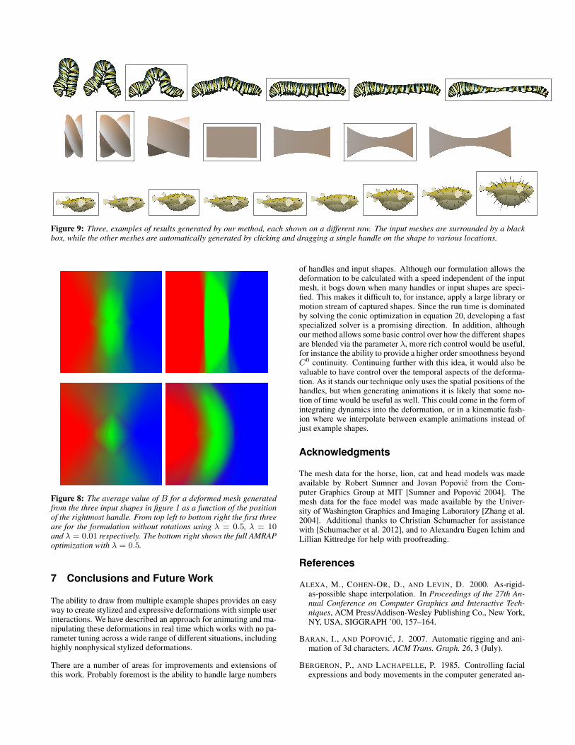
Figure 9: Three, examples of results generated by our method, each shown on a different row. The input meshes are surrounded by a blackbox, while the other meshes are automatically generated by clicking and dragging a single handle on the shape to various locations.

Figure 8: The average value of B for a deformed mesh generatedfrom the three input shapes in figure 1 as a function of the positionof the rightmost handle. From top left to bottom right the first threeare for the formulation without rotations using λ = 0.5, λ = 10and λ = 0.01 respectively. The bottom right shows the full AMRAPoptimization with λ = 0.5.

7 Conclusions and Future Work

The ability to draw from multiple example shapes provides an easyway to create stylized and expressive deformations with simple userinteractions. We have described an approach for animating and ma-nipulating these deformations in real time which works with no pa-rameter tuning across a wide range of different situations, includinghighly nonphysical stylized deformations.

There are a number of areas for improvements and extensions ofthis work. Probably foremost is the ability to handle large numbers

of handles and input shapes. Although our formulation allows thedeformation to be calculated with a speed independent of the inputmesh, it bogs down when many handles or input shapes are speci-fied. This makes it difficult to, for instance, apply a large library ormotion stream of captured shapes. Since the run time is dominatedby solving the conic optimization in equation 20, developing a fastspecialized solver is a promising direction. In addition, althoughour method allows some basic control over how the different shapesare blended via the parameter λ, more rich control would be useful,for instance the ability to provide a higher order smoothness beyondC0 continuity. Continuing further with this idea, it would also bevaluable to have control over the temporal aspects of the deforma-tion. As it stands our technique only uses the spatial positions of thehandles, but when generating animations it is likely that some no-tion of time would be useful as well. This could come in the form ofintegrating dynamics into the deformation, or in a kinematic fash-ion where we interpolate between example animations instead ofjust example shapes.

Acknowledgments

The mesh data for the horse, lion, cat and head models was madeavailable by Robert Sumner and Jovan Popovic from the Com-puter Graphics Group at MIT [Sumner and Popovic 2004]. Themesh data for the face model was made available by the Univer-sity of Washington Graphics and Imaging Laboratory [Zhang et al.2004]. Additional thanks to Christian Schumacher for assistancewith [Schumacher et al. 2012], and to Alexandru Eugen Ichim andLillian Kittredge for help with proofreading.

References

ALEXA, M., COHEN-OR, D., AND LEVIN, D. 2000. As-rigid-as-possible shape interpolation. In Proceedings of the 27th An-nual Conference on Computer Graphics and Interactive Tech-niques, ACM Press/Addison-Wesley Publishing Co., New York,NY, USA, SIGGRAPH ’00, 157–164.

BARAN, I., AND POPOVIC, J. 2007. Automatic rigging and ani-mation of 3d characters. ACM Trans. Graph. 26, 3 (July).

BERGERON, P., AND LACHAPELLE, P. 1985. Controlling facialexpressions and body movements in the computer generated an-

imated short ’Tony de Peltrie’. In SigGraph ’85 Tutorial Notes,Advanced Computer Animation Course.

BOTSCH, M., AND SORKINE, O. 2008. On linear variational sur-face deformation methods. IEEE Transactions on Visualizationand Computer Graphics 14, 1 (Jan.), 213–230.

BOYD, S., AND VANDENBERGHE, L. 2004. Convex Optimization.Cambridge University Press, New York, NY, USA.

CHAO, I., PINKALL, U., SANAN, P., AND SCHRODER, P. 2010.A simple geometric model for elastic deformations. ACM Trans.Graph. 29, 4 (July), 38:1–38:6.

DER, K. G., SUMNER, R. W., AND POPOVIC, J. 2006. In-verse kinematics for reduced deformable models. In ACM SIG-GRAPH 2006 Papers, ACM, New York, NY, USA, SIGGRAPH’06, 1174–1179.

FENG, W.-W., KIM, B.-U., AND YU, Y. 2008. Real-time datadriven deformation using kernel canonical correlation analysis.ACM Transactions on Graphics (TOG) 27, 3, 91.

FROHLICH, S., AND BOTSCH, M. 2011. Example-driven defor-mations based on discrete shells. Computer Graphics Forum 30,8, 2246–2257.

GAO, L., LAI, Y.-K., HUANG, Q.-X., AND HU, S.-M. 2013. Adata-driven approach to realistic shape morphing. In Computergraphics forum, vol. 32, Wiley Online Library, 449–457.

GILL, P. E., MURRAY, W., AND SAUNDERS, M. A. 1997. Snopt:An sqp algorithm for large-scale constrained optimization. SIAMJOURNAL ON OPTIMIZATION 12, 979–1006.

GROCHOW, K., MARTIN, S. L., HERTZMANN, A., ANDPOPOVIC, Z. 2004. Style-based inverse kinematics. ACM Trans.Graph. 23, 3 (Aug.), 522–531.

HAHN, F., THOMASZEWSKI, B., COROS, S., SUMNER, R. W.,COLE, F., MEYER, M., DEROSE, T., AND GROSS, M. 2014.Subspace clothing simulation using adaptive bases. ACM Trans.Graph. 33, 4 (July), 105:1–105:9.

HUANG, H., ZHAO, L., YIN, K., QI, Y., YU, Y., AND TONG,X. 2011. Controllable hand deformation from sparse ex-amples with rich details. In Proceedings of the 2011 ACMSIGGRAPH/Eurographics Symposium on Computer Animation,ACM, New York, NY, USA, SCA ’11, 73–82.

IGARASHI, T., MOSCOVICH, T., AND HUGHES, J. F. 2005. As-rigid-as-possible shape manipulation. ACM Trans. Graph. 24, 3(July), 1134–1141.

JACOBSON, A., BARAN, I., POPOVIC, J., AND SORKINE, O.2011. Bounded biharmonic weights for real-time deforma-tion. ACM Transactions on Graphics (proceedings of ACM SIG-GRAPH) 30, 4, 78:1–78:8.

JACOBSON, A., BARAN, I., KAVAN, L., POPOVIC, J., ANDSORKINE, O. 2012. Fast automatic skinning transforma-tions. ACM Transactions on Graphics (proceedings of ACM SIG-GRAPH) 31, 4, 77:1–77:10.

JACOBSON, A., WEINKAUF, T., AND SORKINE, O. 2012.Smooth shape-aware functions with controlled extrema. Com-puter Graphics Forum (proceedings of EUROGRAPHICS/ACMSIGGRAPH Symposium on Geometry Processing) 31, 5, 1577–1586.

JONES, B., POPOVIC, J., MCCANN, J., LI, W., AND BARGTEIL,A. 2013. Dynamic sprites. In Proceedings of Motion on Games,ACM, New York, NY, USA, MIG ’13, 17:39–17:46.

JONES, B., THUEREY, N., SHINAR, T., AND BARGTEIL, A. W.2016. Example-based plastic deformation of rigid bodies. ACMTrans. on Graphics 35, 4 (July).

KILIAN, M., MITRA, N. J., AND POTTMANN, H. 2007. Geomet-ric modeling in shape space. ACM Trans. Graph. 26, 3 (July).

KOYAMA, Y., TAKAYAMA, K., UMETANI, N., AND IGARASHI,T. 2012. Real-time example-based elastic deformation. In Pro-ceedings of the ACM SIGGRAPH/Eurographics Symposium onComputer Animation, Eurographics Association, Aire-la-Ville,Switzerland, Switzerland, SCA ’12, 19–24.

LEVI, Z., AND GOTSMAN, C. 2015. Smooth rotation enhancedas-rigid-as-possible mesh animation. 264–277.

LEWIS, J. P., AND ANJYO, K.-I. 2010. Direct manipulation blend-shapes. IEEE Comput. Graph. Appl. 30, 4 (July), 42–50.

LEWIS, J. P., CORDNER, M., AND FONG, N. 2000. Posespace deformation: a unified approach to shape interpolationand skeleton-driven deformation. In Proceedings of the 27thannual conference on Computer graphics and interactive tech-niques, ACM Press/Addison-Wesley Publishing Co., 165–172.

LIU, L., ZHANG, L., XU, Y., GOTSMAN, C., AND GORTLER,S. J. 2008. A local/global approach to mesh parameterization.In Proceedings of the Symposium on Geometry Processing, Eu-rographics Association, Aire-la-Ville, Switzerland, Switzerland,SGP ’08, 1495–1504.

MARTIN, S., THOMASZEWSKI, B., GRINSPUN, E., AND GROSS,M. 2011. Example-based elastic materials. ACM Trans. Graph.30, 4 (July), 72:1–72:8.

MILLIEZ, A., WAND, M., CANI, M.-P., AND SEIDEL, H.-P.2013. Mutable elastic models for sculpting structured shapes.In Computer Graphics Forum, vol. 32, Wiley Online Library,21–30.

NIETO, J., AND SUSN, A. 2013. Cage based deformations: A sur-vey. In Deformation Models, M. Gonzlez Hidalgo, A. Mir Tor-res, and J. Varona Gmez, Eds., vol. 7 of Lecture Notes in Compu-tational Vision and Biomechanics. Springer Netherlands, 75–99.

SCHUMACHER, C., THOMASZEWSKI, B., COROS, S., MARTIN,S., SUMNER, R., AND GROSS, M. 2012. Efficient simulationof example-based materials. In Proceedings of the ACM SIG-GRAPH/Eurographics Symposium on Computer Animation, Eu-rographics Association, Aire-la-Ville, Switzerland, Switzerland,SCA ’12, 1–8.

SEDERBERG, T. W., AND PARRY, S. R. 1986. Free-form defor-mation of solid geometric models. SIGGRAPH Comput. Graph.20, 4 (Aug.), 151–160.

SEO, J., IRVING, G., LEWIS, J. P., AND NOH, J. 2011. Com-pression and direct manipulation of complex blendshape models.ACM Trans. Graph. 30, 6 (Dec.), 164:1–164:10.

SHEFFER, A., AND KRAEVOY, V. 2004. Pyramid coordinatesfor morphing and deformation. In Proceedings of the 3D DataProcessing, Visualization, and Transmission, 2Nd InternationalSymposium, IEEE Computer Society, Washington, DC, USA,3DPVT ’04, 68–75.

SLOAN, P.-P. J., ROSE III, C. F., AND COHEN, M. F. 2001.Shape by example. In Proceedings of the 2001 symposium onInteractive 3D graphics, ACM, 135–143.

SONG, C., ZHANG, H., WANG, X., HAN, J., AND WANG, H.2014. Fast corotational simulation for example-driven deforma-tion. Computers & Graphics 40, 49–57.

SORKINE, O., AND ALEXA, M. 2007. As-rigid-as-possible sur-face modeling. In Proceedings of the Fifth Eurographics Sympo-sium on Geometry Processing, Eurographics Association, Aire-la-Ville, Switzerland, Switzerland, SGP ’07, 109–116.

SUMNER, R. W., AND POPOVIC, J. 2004. Deformation transferfor triangle meshes. ACM Trans. Graph. 23, 3 (Aug.), 399–405.

SUMNER, R. W., ZWICKER, M., GOTSMAN, C., AND POPOVIC,J. 2005. Mesh-based inverse kinematics. In ACM SIGGRAPH2005 Papers, ACM, New York, NY, USA, SIGGRAPH ’05,488–495.

TWIGG, C. D., AND KACIC-ALESIC, Z. 2010. Point cloud glue:Constraining simulations using the procrustes transform. In Pro-ceedings of the 2010 ACM SIGGRAPH/Eurographics Sympo-sium on Computer Animation, Eurographics Association, Aire-la-Ville, Switzerland, Switzerland, SCA ’10, 45–54.

WANG, Y., JACOBSON, A., BARBIC, J., AND KAVAN, L. 2015.Linear subspace design for real-time shape deformation. ACMTrans. Graph. 34, 4.

WAREHAM, R., AND LASENBY, J. 2008. Bone glow: An im-proved method for the assignment of weights for mesh deforma-tion. In AMDO, Springer, F. J. P. Lpez and R. B. Fisher, Eds.,vol. 5098 of Lecture Notes in Computer Science, 63–71.

WEBER, O., SORKINE, O., LIPMAN, Y., AND GOTSMAN, C.2007. Context-aware skeletal shape deformation. In ComputerGraphics Forum, vol. 26, Wiley Online Library, 265–274.

ZHANG, L., SNAVELY, N., CURLESS, B., AND SEITZ, S. M.2004. Spacetime faces: High resolution capture for modelingand animation. ACM Trans. Graph. 23, 3 (Aug.), 548–558.

ZHANG, W., ZHENG, J., AND THALMANN, N. M. 2015. Real-Time Subspace Integration for Example-Based Elastic Material.Computer Graphics Forum.

A Trust Region Optimization

Although it normally works well in practice, the alternating mini-mization is section 5 is not guaranteed to converge because the stepsolving for T and B and the step solving for R do so by minimiz-ing different energies. To guarantee convergence the nonlinearitiesintroduced by the solution for R can be incorporated into the solu-tion for T and B. As this adds a non-trivial additional complexityto the optimizer to cover relatively rare failure cases, we recom-mend that anyone implementing an AMRAP solver do so first asdescribed in section 5, and only implement the additions here if itappears necessary to do so.

As T and B are updated, the value of R changes according toequation 22. To account for this, we linearize the effect of Ron E(T, B,R,P ) and minimize equation 20 with a trust regionapproach. This linearization approximates E in the vicinity ofR ≈ R0 as:

E(T, B,R,P ) ≈E(T, B,R0,P ) + ∂RE (24)

Where ∂RE is the linearization of the effect the R has on E as T

and B vary and can be simplified as:

∂RE =1

2√

Ed(T, B,R,P )∂REd (25)

=1

4√

Ed(T, B,R,P )∂REd3 (26)

Where the last equality results from observing that Ed1 is indepen-dent of R and that the definition of R via equation 22 means that∂REd2 = 0. Letting x represent a single parameter of T and usingequation 18 gives:

∂REd3 =∑gs1s2

Bgs1Bgs2 tr (Hgs1s2dRgs1s2) (27)

with

dRgs1s2 =RTgs2 (∂xRgs1) + (∂xRgs2)

T Rgs1 (28)

where ∂xRgs is calculated as described as described by Twigg andKacic-Alesic [2010]:

∂xRgs = UΩVT (29)

where U and V come from the singular value decomposition ofKgs and Ω is a k × k matrix such that:

Ωij =

[UT

(∂xKgs

)V]ij−

[UT

(∂xKgs

)V]ji

Dii +Djj(30)

The term ∂xKgs in this equation represents the partial derivativeof Kgs with respect to x and is straightforward to compute by dif-ferentiating equation 23.

To complete the algorithm solving for T and B, we start withan initial guess T0, B0 and minimize equation 24 subject tothe constraints in equation 20 and the additional constraint that∥vec(T, B)− vec(T0, B0)∥ ≤ r. The scalar r is a trust radiusensuring that the optimization converges, and a sufficiently smallvalue of r guarantees a decrease in the optimization’s objectivefunction. This optimization is another SOCP which may solvedwith the same technique as equation 20.

The trust radius r starts at r = 1 and varies dynamically duringthe course of the optimization. If solving for T and B then recom-puting R yields a decrease in E, then we update r′ = max(ρr, 1)and proceed. Otherwise we set r′ = max(ρ−1r, 1) and re-solve.We use the relatively aggressive value ρ = 10 as a reflection ofthe empirical observation that the trust region is rarely necessary,but when it is r normally needs to be relatively small to ensure adecrease in E.