Fast and Flexible ADMM Algorithms for Trend Filtering

Aaditya Ramdas21

aramdas@cs.cmu.edu

Ryan J. Tibshirani12

ryantibs@stat.cmu.edu

1Department of Statistics and 2Machine Learning DepartmentCarnegie Mellon University

Abstract

This paper presents a fast and robust algorithm for trend filtering, a recently developednonparametric regression tool. It has been shown that, for estimating functions whose deriva-tives are of bounded variation, trend filtering achieves the minimax optimal error rate, whileother popular methods like smoothing splines and kernels do not. Standing in the way of amore widespread practical adoption, however, is a lack of scalable and numerically stable al-gorithms for fitting trend filtering estimates. This paper presents a highly efficient, specializedADMM routine for trend filtering. Our algorithm is competitive with the specialized interiorpoint methods that are currently in use, and yet is far more numerically robust. Furthermore,the proposed ADMM implementation is very simple, and importantly, it is flexible enough toextend to many interesting related problems, such as sparse trend filtering and isotonic trendfiltering. Software for our method is freely available, in both the C and R languages.

1 Introduction

Trend filtering is a relatively new method for nonparametric regression, proposed independently bySteidl et al. (2006), Kim et al. (2009). Suppose that we are given output points y = (y1, . . . yn) ∈ Rn,observed across evenly spaced input points x = (x1, . . . xn) ∈ Rn, say, x1 = 1, . . . xn = n forsimplicity. The trend filtering estimate β = (β1, . . . βn) ∈ Rn of a specified order k ≥ 0 is defined as

β = argminβ∈Rn

1

2‖y − β‖22 + λ‖D(k+1)β‖1. (1)

Here λ ≥ 0 is a tuning parameter, and D(k+1) ∈ R(n−k)×n is the discrete difference (or derivative)operator of order k + 1. We can define these operators recursively as

D(1) =

−1 1 0 . . . 0 0

0 −1 1 . . . 0 0...0 0 0 . . . −1 1

, (2)

andD(k+1) = D(1)D(k) for k = 1, 2, 3, . . . . (3)

(Note that, above, we write D(1) to mean the (n−k−1)× (n−k) version of the 1st order differencematrix in (2).) When k = 0, we can see from the definition of D(1) in (2) that the trend filteringproblem (1) is the same as the 1-dimensional fused lasso problem (Tibshirani et al. 2005), also called1-dimensional total variation denoising (Rudin et al. 1992), and hence the 0th order trend filteringestimate β is piecewise constant across the input points x1, . . . xn.

1

For a general k, the kth order trend filtering estimate has the structure of a kth order piecewisepolynomial function, evaluated across the inputs x1, . . . xn. The knots in this piecewise polynomialare selected adaptively among x1, . . . xn, with a higher value of the tuning parameter λ (generally)corresponding to fewer knots. To see examples, the reader can jump ahead to the next subsection,or to future sections. For arbitrary input points x1, . . . xn (i.e., these need not be evenly spaced), thedefined difference operators will have different nonzero entries, but their structure and the recursiverelationship between them is basically the same; see Section 4.

Broadly speaking, nonparametric regression is a well-studied field with many celebrated tools,and so one may wonder about the merits of trend filtering in particular. For detailed motivation,we refer the reader to Tibshirani (2014), where it is argued that trend filtering essentially balancesthe strengths of smoothing splines (de Boor 1978, Wahba 1990) and locally adaptive regressionsplines (Mammen & van de Geer 1997), which are two of the most common tools for piecewisepolynomial estimation. In short: smoothing splines are highly computationally efficient but arenot minimax optimal (for estimating functions whose derivatives are of bounded variation); locallyadaptive regression splines are minimax optimal but are relatively inefficient in terms of computation;trend filtering is both minimax optimal and computationally comparable to smoothing splines.Tibshirani (2014) focuses mainly on the statistical properties trend filtering estimates, and relies onexternally derived algorithms for comparisons of computational efficiency.

1.1 Overview of contributions

In this paper, we propose a new algorithm for trend filtering. We do not explicitly address theproblem of model selection, i.e., we do not discuss how to choose the tuning parameter λ in (1),which is a long-standing statistical issue with any regularized estimation method. Our concern iscomputational; if a practitioner wants to solve the trend filtering problem (1) at a given value of λ(or sequence of values), then we provide a scalable and efficient means of doing so. Of course, a fastalgorithm such as the one we provide can still be helpful for model selection, in that it can providespeedups for common techniques like cross-validation.

For 0th order trend filtering, i.e., the 1d fused lasso problem, two direct, linear time algorithmsalready exist: the first uses a taut string principle (Davies & Kovac 2001), and the second uses anentirely different dynamic programming approach (Johnson 2013). Both are extremely (and equally)fast in practice, and for this special 0th order problem, these two direct algorithms rise above all elsein terms of computational efficiency and numerical accuracy. As far as we know (and despite ourbest attempts), these algorithms cannot be directly extended to the higher order cases k = 1, 2, 3, . . ..However, our proposal indirectly extends these formidable algorithms to the higher order cases witha special implementation of the alternating direction method of multipliers (ADMM). In general,there can be multiple ways to reparametrize an unconstrained optimization problem so that ADMMcan be applied; for the trend filtering problem (1), we choose a particular parametrization suggestedby the recursive decomposition (3), leveraging the fast, exact algorithms that exist for the k = 0case. We find that this choice makes a big difference in terms of the convergence of the resultingADMM routine, compared to what may be considered the standard ADMM parametrization for (1).

Currently, the specialized primal-dual interior point (PDIP) method of Kim et al. (2009) seemsto be the preferred method for computing trend filtering estimates. The iterations of this algorithmare cheap because they reduce to solving banded linear systems (the discrete difference operators arethemselves banded). Our specialized ADMM implementation and the PDIP method have distinctstrengths. We summarize our main findings below.

• Our specialized ADMM implementation converges more reliably than the PDIP method, overa wide range of problems sizes n and tuning parameter values λ.

• In particular setups—namely, small problem sizes, and small values of λ for moderate andlarge problem sizes—the PDIP method converges to high accuracy solutions very rapidly. In

2

such situations, our specialized ADMM algorithm does not match the convergence rate of thissecond-order method.

• However, when plotting the function estimates, our specialized ADMM implementation pro-duces solutions of visually perfectly acceptable accuracy after a small number of iterations.This is true over a broad range of problem sizes n and parameter values λ, and covers the set-tings in which its achieved criterion value has not converged at the rate of the PDIP method.

• Furthermore, our specialized ADMM implementation displays a greatly improved convergencerate over what may be thought of as the “standard” ADMM implementation for problem (1).Loosely speaking, standard implementations of ADMM are generally considered to behavelike first-order methods (Boyd et al. 2011), whereas our specialized implementation exhibitsperformance somewhere in between that of a first- and second-order method.

• One iteration of our specialized ADMM implementation has linear complexity in the problemsize n; this is also true for PDIP. Empirically, an iteration of our ADMM routine runs about10 times faster than a PDIP iteration.

• Our specialized ADMM implementation is quite simple (considerably simpler than the spe-cialized primal-dual interior point method), and is flexible enough that it can be extended tocover many variants and extensions of the basic trend filtering problem (1), such as sparsetrend filtering, mixed trend filtering, and isotonic trend filtering.

• Finally, it is worth remarking that extensions beyond the univariate case are readily available aswell, as univariate nonparametric regression tools can be used as building blocks for estimationin broader model classes, e.g., in generalized additive models (Hastie & Tibshirani 1990).

Readers well-versed in optimization may wonder about alternative iterative (descent) methodsfor solving the trend filtering problem (1). Two natural candidates that have enjoyed much successin lasso regression problems are proximal gradient and coordinate descent algorithms. Next, wegive a motivating case study that illustrates the inferior performance of both of these methods fortrend filtering. In short, their performance is heavily affected by poor conditioning of the differenceoperator D(k+1), and their convergence is many orders of magnitude worse than the specializedprimal-dual interior point and ADMM approaches.

1.2 A motivating example

Conditioning is a subtle but ever-present issue faced by iterative (indirect) optimization methods.This issue affects some algorithms more than others; e.g., in a classical optimization context, itis well-understood that the convergence bounds for gradient descent depend on the smallest andlargest eigenvalues of the Hessian of the criterion function, while those for Newton’s method donot (Newton’s method being affine invariant). Unfortunately, conditioning is a very real issue whensolving the trend filtering problem in (1)—the discrete derivative operators D(k+1), k = 0, 1, 2, . . .are extremely ill-conditioned, and this only worsens as k increases.

This worry can be easily realized in examples, as we now demonstrate in a simple simulationwith a reasonable polynomial order, k = 1, and a modest problem size, n = 1000. For solving thetrend filtering problem (1), with λ = 1000, we compare proximal gradient descent and acceleratedproximal gradient method (performed on both the primal and the dual problems), coordinate descent,a standard ADMM approach, our specialized ADMM approach, and the specialized PDIP methodof Kim et al. (2009). Details of the simulation setup and these various algorithms are given inAppendix A.1, but the main message can be seen from Figure 1. Different variants of proximalgradient methods, as well as coordinate descent, and a standard ADMM approach, all perform quitepoorly in computing trend filtering estimate, but the second-order PDIP method and our specialized

3

ADMM implementation perform drastically better—these two reach in 20 iterations what the otherscould not reach in many thousands. Although the latter two techniques perform similarly in thisexample, we will see later that our specialized ADMM approach generally suffers from far lessconditioning and convergence issues than PDIP, especially in regimes of regularization (i.e., rangesof λ values) that are most interesting statistically.

The rest of this paper is organized as follows. In Section 2, we describe our specialized ADMMimplementation for trend filtering. In Section 3, we make extensive comparisons to PDIP. Section4 covers the case of general input points x1, . . . xn. Section 5 considers several extensions of thebasic trend filtering model, and the accompanying adaptions of our specialized ADMM algorithm.Section 6 concludes with a short discussion.

2 A specialized ADMM algorithm

We describe a specialized ADMM algorithm for trend filtering. This algorithm may appear to onlyslightly differ in its construction from a more standard ADMM algorithm for trend filtering, andboth approaches have virtually the same computational complexity, requiring O(n) operations periteration; however, as we have glimpsed in Figure 1, the difference in convergence between the twois drastic.

The standard ADMM approach (e.g., Boyd et al. (2011)) is based on rewriting problem (1) as

minβ∈Rn, α∈Rn−k−1

1

2‖y − β‖22 + λ‖α‖1 subject to α = D(k+1)β. (4)

The augmented Lagrangian can then be written as

L(β, α, u) =1

2‖y − β‖22 + λ‖α‖1 +

ρ

2‖α−D(k+1)β + u‖22 −

ρ

2‖u‖22,

from which we can derive the standard ADMM updates:

β ←(I + ρ(D(k+1))TD(k+1)

)−1(y + ρ(D(k+1))T (α+ u)

), (5)

α← Sλ/ρ(D(k+1)β − u), (6)

u← u+ α−D(k+1)β. (7)

The β-update is a banded linear system solve, with bandwidth k + 2, and can be implemented intime O(n(k+2)2) (actually, O(n(k+2)2) for the first solve, with a banded Cholesky, and O(n(k+2))for each subsequent solve). The α-update, where Sλ/ρ denotes coordinate-wise soft-thresholding atthe level λ/ρ, takes time O(n−k−1). The dual update uses a banded matrix multiplication, takingtime O(n(k+ 2)), and therefore one full iteration of standard ADMM updates can be done in lineartime (considering k as a constant).

Our specialized ADMM approach instead begins by rewriting (1) as

minβ∈Rn, α∈Rn−k

1

2‖y − β‖22 + λ‖D(1)α‖1 subject to α = D(k)β, (8)

where we have used the recursive property D(k+1) = D(1)D(k). The augmented Lagrangian is now

L(β, α, u) =1

2‖y − β‖22 + λ‖D(1)α‖1 +

ρ

2‖α−D(k)β + u‖22 −

ρ

2‖u‖22,

yielding the specialized ADMM updates:

β ←(I + ρ(D(k))TD(k)

)−1(y + ρ(D(k))T (α+ u)

), (9)

α← argminα∈Rn−k

1

2‖D(k)β − u− α‖22 + λ/ρ‖D(1)α‖1, (10)

u← u+ α−D(k)β. (11)

4

●

●

●●

●

●

●

●●

●

●

●●

●●●

●

●

●

●

●

●●

●

●

●

●

●

●

●●●●●

●

●●

●

●

●

●

●

●●●●●

●●

●

●

●

●

●

●●●

●

●

●

●●

●

●

●

●

●

●●●●●

●

●

●

●

●●

●

●

●

●●

●●●

●

●

●

●

●

●

●

●

●●●

●

●

●●

●●

●

●

●

●

●

●

●

●

●

●●

●

●

●

●●●●●

●●●

●●

●

●

●

●

●

●

●

●

●●●●●

●

●●

●●●●

●

●

●

●

●

●

●

●

●

●

●

●●

●

●

●

●

●●

●

●

●

●

●

●

●●●

●

●

●●

●

●●●

●●

●●

●

●

●

●●

●

●

●

●

●

●●●

●●

●

●●

●

●

●

●

●

●

●

●

●

●●

●

●

●

●

●

●

●

●

●

●

●

●

●

●

●

●●

●

●

●

●

●

●

●

●

●

●

●

●

●

●

●

●●

●

●●

●

●

●●

●

●

●●●

●

●

●

●

●

●

●

●

●

●

●

●

●

●

●

●

●

●

●

●

●●●

●

●

●

●●

●

●

●

●●●

●

●●●●

●

●

●

●

●

●●●●

●

●●

●●

●

●

●

●

●

●

●●●

●●

●

●

●

●

●●

●●

●

●●●●

●

●

●

●●●

●

●●●

●

●

●

●

●

●●

●

●

●

●

●

●●●

●

●

●

●

●

●

●

●

●●

●

●

●

●●●

●

●●●

●●●

●

●

●

●

●

●

●●

●●

●

●●●

●

●●

●

●

●

●

●

●

●●

●

●

●

●

●

●

●

●

●

●

●●

●

●

●

●

●

●

●●

●

●

●

●

●

●

●

●

●

●●●●

●

●

●

●

●

●

●

●

●

●

●

●

●

●

●

●

●

●

●

●●

●

●

●

●●

●

●●

●●

●

●

●●

●

●

●

●

●

●

●

●

●

●

●

●

●●●

●●

●

●

●●

●

●

●

●●●

●

●

●●

●●●

●

●

●

●

●

●

●●

●●●

●

●

●

●

●

●

●

●

●

●

●

●

●●

●

●●

●

●

●

●

●

●

●

●

●

●●

●

●●

●●●

●●●●●

●●

●

●

●

●

●●●

●

●

●●

●

●●

●●●●●●

●

●

●

●

●

●●

●

●

●

●

●

●

●

●

●●

●●

●●

●

●

●●

●

●

●

●

●

●

●

●

●

●

●

●

●

●

●●

●

●

●

●

●●

●

●

●●

●

●●

●

●●

●

●

●

●

●●●

●

●

●

●

●●●

●●

●

●

●

●

●

●

●●

●●

●

●●●●●

●

●

●●

●

●●

●

●●

●

●

●

●●

●●

●●

●

●

●

●

●

●

●●

●

●

●

●

●●●●●

●

●

●

●

●●

●●

●

●

●

●

●●

●

●

●

●

●

●

●●●

●

●

●

●

●●

●

●

●●

●

●

●

●●

●

●

●

●●

●●●

●

●●●

●

●

●●

●

●

●●

●●

●

●

●●

●

●

●

●

●

●●

●

●●

●

●

●

●

●

●●

●

●●●

●

●●

●

●●

●

●●

●

●●

●

●

●

●

●

●●

●

●

●

●

●

●

●

●●●

●

●

●

●●

●

●●

●

●

●

●

●

●

●

●

●

●●●●

●

●●

●

●

●

●●

●

●●●

●

●

●

●

●

●

●

●

●

●●

●

●

●

●

●

●

●

●

●

●

●

●

●●●●

●●●

●●

●●●

●●

●

●●●

●●●

●●

●

●●

●

●

●

●

●

●●●

●

●

●

●●

●

●

●

●

●

●●

●●

●

●

●

●

●

●●●

●

●●

●

●

●●●●

●

●

●

●

●

●

●

●

●

●●

●

●

●

●

●

●

●

●●

●●

●

●

●

●

●●

●

●●

●

●●

●

●

●●

●

●

●

●

●

●

●●

●●●

●

●

●●

●

0 200 400 600 800 1000

05

10

ExactDual PGDual APG

●

●

●●

●

●

●

●●

●

●

●●

●●●

●

●

●

●

●

●●

●

●

●

●

●

●

●●●●●

●

●●

●

●

●

●

●

●●●●●

●●

●

●

●

●

●

●●●

●

●

●

●●

●

●

●

●

●

●●●●●

●

●

●

●

●●

●

●

●

●●

●●●

●

●

●

●

●

●

●

●

●●●

●

●

●●

●●

●

●

●

●

●

●

●

●

●

●●

●

●

●

●●●●●

●●●

●●

●

●

●

●

●

●

●

●

●●●●●

●

●●

●●●●

●

●

●

●

●

●

●

●

●

●

●

●●

●

●

●

●

●●

●

●

●

●

●

●

●●●

●

●

●●

●

●●●

●●

●●

●

●

●

●●

●

●

●

●

●

●●●

●●

●

●●

●

●

●

●

●

●

●

●

●

●●

●

●

●

●

●

●

●

●

●

●

●

●

●

●

●

●●

●

●

●

●

●

●

●

●

●

●

●

●

●

●

●

●●

●

●●

●

●

●●

●

●

●●●

●

●

●

●

●

●

●

●

●

●

●

●

●

●

●

●

●

●

●

●

●●●

●

●

●

●●

●

●

●

●●●

●

●●●●

●

●

●

●

●

●●●●

●

●●

●●

●

●

●

●

●

●

●●●

●●

●

●

●

●

●●

●●

●

●●●●

●

●

●

●●●

●

●●●

●

●

●

●

●

●●

●

●

●

●

●

●●●

●

●

●

●

●

●

●

●

●●

●

●

●

●●●

●

●●●

●●●

●

●

●

●

●

●

●●

●●

●

●●●

●

●●

●

●

●

●

●

●

●●

●

●

●

●

●

●

●

●

●

●

●●

●

●

●

●

●

●

●●

●

●

●

●

●

●

●

●

●

●●●●

●

●

●

●

●

●

●

●

●

●

●

●

●

●

●

●

●

●

●

●●

●

●

●

●●

●

●●

●●

●

●

●●

●

●

●

●

●

●

●

●

●

●

●

●

●●●

●●

●

●

●●

●

●

●

●●●

●

●

●●

●●●

●

●

●

●

●

●

●●

●●●

●

●

●

●

●

●

●

●

●

●

●

●

●●

●

●●

●

●

●

●

●

●

●

●

●

●●

●

●●

●●●

●●●●●

●●

●

●

●

●

●●●

●

●

●●

●

●●

●●●●●●

●

●

●

●

●

●●

●

●

●

●

●

●

●

●

●●

●●

●●

●

●

●●

●

●

●

●

●

●

●

●

●

●

●

●

●

●

●●

●

●

●

●

●●

●

●

●●

●

●●

●

●●

●

●

●

●

●●●

●

●

●

●

●●●

●●

●

●

●

●

●

●

●●

●●

●

●●●●●

●

●

●●

●

●●

●

●●

●

●

●

●●

●●

●●

●

●

●

●

●

●

●●

●

●

●

●

●●●●●

●

●

●

●

●●

●●

●

●

●

●

●●

●

●

●

●

●

●

●●●

●

●

●

●

●●

●

●

●●

●

●

●

●●

●

●

●

●●

●●●

●

●●●

●

●

●●

●

●

●●

●●

●

●

●●

●

●

●

●

●

●●

●

●●

●

●

●

●

●

●●

●

●●●

●

●●

●

●●

●

●●

●

●●

●

●

●

●

●

●●

●

●

●

●

●

●

●

●●●

●

●

●

●●

●

●●

●

●

●

●

●

●

●

●

●

●●●●

●

●●

●

●

●

●●

●

●●●

●

●

●

●

●

●

●

●

●

●●

●

●

●

●

●

●

●

●

●

●

●

●

●●●●

●●●

●●

●●●

●●

●

●●●

●●●

●●

●

●●

●

●

●

●

●

●●●

●

●

●

●●

●

●

●

●

●

●●

●●

●

●

●

●

●

●●●

●

●●

●

●

●●●●

●

●

●

●

●

●

●

●

●

●●

●

●

●

●

●

●

●

●●

●●

●

●

●

●

●●

●

●●

●

●●

●

●

●●

●

●

●

●

●

●

●●

●●●

●

●

●●

●

0 200 400 600 800 10000

510

ExactLasso PGLasso APG

●

●

●●

●

●

●

●●

●

●

●●

●●●

●

●

●

●

●

●●

●

●

●

●

●

●

●●●●●

●

●●

●

●

●

●

●

●●●●●

●●

●

●

●

●

●

●●●

●

●

●

●●

●

●

●

●

●

●●●●●

●

●

●

●

●●

●

●

●

●●

●●●

●

●

●

●

●

●

●

●

●●●

●

●

●●

●●

●

●

●

●

●

●

●

●

●

●●

●

●

●

●●●●●

●●●

●●

●

●

●

●

●

●

●

●

●●●●●

●

●●

●●●●

●

●

●

●

●

●

●

●

●

●

●

●●

●

●

●

●

●●

●

●

●

●

●

●

●●●

●

●

●●

●

●●●

●●

●●

●

●

●

●●

●

●

●

●

●

●●●

●●

●

●●

●

●

●

●

●

●

●

●

●

●●

●

●

●

●

●

●

●

●

●

●

●

●

●

●

●

●●

●

●

●

●

●

●

●

●

●

●

●

●

●

●

●

●●

●

●●

●

●

●●

●

●

●●●

●

●

●

●

●

●

●

●

●

●

●

●

●

●

●

●

●

●

●

●

●●●

●

●

●

●●

●

●

●

●●●

●

●●●●

●

●

●

●

●

●●●●

●

●●

●●

●

●

●

●

●

●

●●●

●●

●

●

●

●

●●

●●

●

●●●●

●

●

●

●●●

●

●●●

●

●

●

●

●

●●

●

●

●

●

●

●●●

●

●

●

●

●

●

●

●

●●

●

●

●

●●●

●

●●●

●●●

●

●

●

●

●

●

●●

●●

●

●●●

●

●●

●

●

●

●

●

●

●●

●

●

●

●

●

●

●

●

●

●

●●

●

●

●

●

●

●

●●

●

●

●

●

●

●

●

●

●

●●●●

●

●

●

●

●

●

●

●

●

●

●

●

●

●

●

●

●

●

●

●●

●

●

●

●●

●

●●

●●

●

●

●●

●

●

●

●

●

●

●

●

●

●

●

●

●●●

●●

●

●

●●

●

●

●

●●●

●

●

●●

●●●

●

●

●

●

●

●

●●

●●●

●

●

●

●

●

●

●

●

●

●

●

●

●●

●

●●

●

●

●

●

●

●

●

●

●

●●

●

●●

●●●

●●●●●

●●

●

●

●

●

●●●

●

●

●●

●

●●

●●●●●●

●

●

●

●

●

●●

●

●

●

●

●

●

●

●

●●

●●

●●

●

●

●●

●

●

●

●

●

●

●

●

●

●

●

●

●

●

●●

●

●

●

●

●●

●

●

●●

●

●●

●

●●

●

●

●

●

●●●

●

●

●

●

●●●

●●

●

●

●

●

●

●

●●

●●

●

●●●●●

●

●

●●

●

●●

●

●●

●

●

●

●●

●●

●●

●

●

●

●

●

●

●●

●

●

●

●

●●●●●

●

●

●

●

●●

●●

●

●

●

●

●●

●

●

●

●

●

●

●●●

●

●

●

●

●●

●

●

●●

●

●

●

●●

●

●

●

●●

●●●

●

●●●

●

●

●●

●

●

●●

●●

●

●

●●

●

●

●

●

●

●●

●

●●

●

●

●

●

●

●●

●

●●●

●

●●

●

●●

●

●●

●

●●

●

●

●

●

●

●●

●

●

●

●

●

●

●

●●●

●

●

●

●●

●

●●

●

●

●

●

●

●

●

●

●

●●●●

●

●●

●

●

●

●●

●

●●●

●

●

●

●

●

●

●

●

●

●●

●

●

●

●

●

●

●

●

●

●

●

●

●●●●

●●●

●●

●●●

●●

●

●●●

●●●

●●

●

●●

●

●

●

●

●

●●●

●

●

●

●●

●

●

●

●

●

●●

●●

●

●

●

●

●

●●●

●

●●

●

●

●●●●

●

●

●

●

●

●

●

●

●

●●

●

●

●

●

●

●

●

●●

●●

●

●

●

●

●●

●

●●

●

●●

●

●

●●

●

●

●

●

●

●

●●

●●●

●

●

●●

●

0 200 400 600 800 1000

05

10

ExactCoordinate descStandard ADMM

●

●

●●

●

●

●

●●

●

●

●●

●●●

●

●

●

●

●

●●

●

●

●

●

●

●

●●●●●

●

●●

●

●

●

●

●

●●●●●

●●

●

●

●

●

●

●●●

●

●

●

●●

●

●

●

●

●

●●●●●

●

●

●

●

●●

●

●

●

●●

●●●

●

●

●

●

●

●

●

●

●●●

●

●

●●

●●

●

●

●

●

●

●

●

●

●

●●

●

●

●

●●●●●

●●●

●●

●

●

●

●

●

●

●

●

●●●●●

●

●●

●●●●

●

●

●

●

●

●

●

●

●

●

●

●●

●

●

●

●

●●

●

●

●

●

●

●

●●●

●

●

●●

●

●●●

●●

●●

●

●

●

●●

●

●

●

●

●

●●●

●●

●

●●

●

●

●

●

●

●

●

●

●

●●

●

●

●

●

●

●

●

●

●

●

●

●

●

●

●

●●

●

●

●

●

●

●

●

●

●

●

●

●

●

●

●

●●

●

●●

●

●

●●

●

●

●●●

●

●

●

●

●

●

●

●

●

●

●

●

●

●

●

●

●

●

●

●

●●●

●

●

●

●●

●

●

●

●●●

●

●●●●

●

●

●

●

●

●●●●

●

●●

●●

●

●

●

●

●

●

●●●

●●

●

●

●

●

●●

●●

●

●●●●

●

●

●

●●●

●

●●●

●

●

●

●

●

●●

●

●

●

●

●

●●●

●

●

●

●

●

●

●

●

●●

●

●

●

●●●

●

●●●

●●●

●

●

●

●

●

●

●●

●●

●

●●●

●

●●

●

●

●

●

●

●

●●

●

●

●

●

●

●

●

●

●

●

●●

●

●

●

●

●

●

●●

●

●

●

●

●

●

●

●

●

●●●●

●

●

●

●

●

●

●

●

●

●

●

●

●

●

●

●

●

●

●

●●

●

●

●

●●

●

●●

●●

●

●

●●

●

●

●

●

●

●

●

●

●

●

●

●

●●●

●●

●

●

●●

●

●

●

●●●

●

●

●●

●●●

●

●

●

●

●

●

●●

●●●

●

●

●

●

●

●

●

●

●

●

●

●

●●

●

●●

●

●

●

●

●

●

●

●

●

●●

●

●●

●●●

●●●●●

●●

●

●

●

●

●●●

●

●

●●

●

●●

●●●●●●

●

●

●

●

●

●●

●

●

●

●

●

●

●

●

●●

●●

●●

●

●

●●

●

●

●

●

●

●

●

●

●

●

●

●

●

●

●●

●

●

●

●

●●

●

●

●●

●

●●

●

●●

●

●

●

●

●●●

●

●

●

●

●●●

●●

●

●

●

●

●

●

●●

●●

●

●●●●●

●

●

●●

●

●●

●

●●

●

●

●

●●

●●

●●

●

●

●

●

●

●

●●

●

●

●

●

●●●●●

●

●

●

●

●●

●●

●

●

●

●

●●

●

●

●

●

●

●

●●●

●

●

●

●

●●

●

●

●●

●

●

●

●●

●

●

●

●●

●●●

●

●●●

●

●

●●

●

●

●●

●●

●

●

●●

●

●

●

●

●

●●

●

●●

●

●

●

●

●

●●

●

●●●

●

●●

●

●●

●

●●

●

●●

●

●

●

●

●

●●

●

●

●

●

●

●

●

●●●

●

●

●

●●

●

●●

●

●

●

●

●

●

●

●

●

●●●●

●

●●

●

●

●

●●

●

●●●

●

●

●

●

●

●

●

●

●

●●

●

●

●

●

●

●

●

●

●

●

●

●

●●●●

●●●

●●

●●●

●●

●

●●●

●●●

●●

●

●●

●

●

●

●

●

●●●

●

●

●

●●

●

●

●

●

●

●●

●●

●

●

●

●

●

●●●

●

●●

●

●

●●●●

●

●

●

●

●

●

●

●

●

●●

●

●

●

●

●

●

●

●●

●●

●

●

●

●

●●

●

●●

●

●●

●

●

●●

●

●

●

●

●

●

●●

●●●

●

●

●●

●

0 200 400 600 800 1000

05

10

ExactPDIPSpecial ADMM

Figure 1: All plots show n = 1000 simulated observations in gray and the exact trend filtering solution as ablack line, computed using the dual path algorithm of Tibshirani & Taylor (2011). The top left panel showsproximal gradient descent and its accelerated version applied to the dual problem, after 10,000 iterations.The top right show proximal gradient and its accelerated version after rewriting trend filtering in lasso form,again after 10,000 iterations. The bottom left shows coordinate descent applied to the lasso form, and astandard ADMM approach applied to the original problem, each using 5000 iterations (where one iterationfor coordinate descent is one full cycle of coordinate updates). The bottom right panel shows the specializedPDIP and ADMM algorithms, which only need 20 iterations, and match the exact solution to perfect visualaccuracy. Due to the special form of the problem, all algorithms here have O(n) complexity per iteration(except coordinate descent, which has a higher iteration cost).

5

The β- and u-updates are analogous to those from the standard ADMM, just of a smaller order k.But the α-update above is not; the α-update itself requires solving a constant order trend filteringproblem, i.e., a 1d fused lasso problem. Therefore, the specialized approach would not be efficient if itwere not for the extremely fast, direct solvers that exist for the 1d fused lasso. Two exact, linear time1d fused lasso solvers were given by Davies & Kovac (2001), Johnson (2013). The former is basedon taut strings, and the latter on dynamic programming. Both algorithms are very creative and area marvel in their own right; we are more familiar with the dynamic programming approach, and soin our specialized ADMM algorithm, we utilize (a custom-made, highly-optimized implementationof) this dynamic programming routine for the α-update, hence writing

α← DPλ/ρ(D(k)β − u). (12)

This uses O(n − k) operations, and thus a full round of specialized ADMM updates runs in lineartime, the same as the standard ADMM ones (the two approaches are also empirically very similarin terms of computational time; see Figure 4). As mentioned in the introduction, neither the tautstring nor dynamic programming approach can be directly extended beyond the k = 0 case, tothe best of our knowledge, for solving higher order trend filtering problems; however, they can bewrapped up in the special ADMM algorithm described above, and in this manner, they lend theirefficiency to the computation of higher order estimates.

2.1 Superiority of specialized over standard ADMM

We now provide further experimental evidence that our specialized ADMM implementation sig-nificantly outperforms the naive standard ADMM. We simulated noisy data from three differentunderlying signals: constant, sinusoidal, and Doppler wave signals (representing three broad classesof functions: trivial smoothness, homogeneous smoothness, and inhomogeneous smoothness). Weexamined 9 different problem sizes, spaced roughly logarithmically from n = 500 to n = 500, 000,and considered computation of the trend filtering solution in (1) for the orders k = 1, 2, 3. We alsoconsidered 20 values of λ, spaced logarithmically between λmax and 10−5λmax, where

λmax =∥∥((D(k+1)(D(k+1))T

)−1(D(k+1))T y

∥∥∞,

the smallest value of λ at which the penalty term ‖D(k+1)β‖1 is zero at the solution (and hencethe solution is exactly a kth order polynomial). In each problem instance—indexed by the choiceof underlying function, problem size, polynomial order k, and tuning parameter value λ—we rana large number of iterations of the ADMM algorithms, and recorded the achieved criterion valuesacross iterations.

The results from one particular instance, in which the underlying signal was the Doppler wave,n = 10, 000, and k = 2, are shown in Figure 2; this instance was chosen arbitrarily, and we havefound the same qualitative behavior to persist throughout the entire simulation suite. We can seeclearly that in each regime of regularization, the specialized routine dominates the standard one interms of convergence to optimum. Again, we reiterate that qualitatively the same conclusion holdsacross all simulation parameters, and the gap between the specialized and standard approachesgenerally widens as the polynomial order k increases.

2.2 Some intuition for specialized versus standard ADMM

One may wonder why the two algorithms, standard and specialized ADMM, differ so significantlyin terms of their performance. Here we provide some intuition with regard to this question. A first,very rough interpretation: the specialized algorithm utilizes a dynamic programming subroutine(12) in place of soft-thresholding (6), therefore solving a more “difficult” subproblem in the sameamount of time (linear in the input size), and likely making more progress towards minimizing the

6

0 50 100 150 200 250

5e+

035e

+04

5e+

055e

+06

Iteration

Crit

erio

nStandard ADMMSpecial ADMM

0 50 100 150 200 250

1e+

035e

+03

5e+

045e

+05

Iteration

Crit

erio

n

Standard ADMMSpecial ADMM

0 50 100 150 200 250

5e+

022e

+03

1e+

045e

+04

2e+

05

Iteration

Crit

erio

n

Standard ADMMSpecial ADMM

Figure 2: All plots show values of the trend filtering criterion versus iteration number in the two ADMMimplementations. The underlying signal here was the Doppler wave, with n = 10, 000, and k = 2. Theleft plot shows a large value of λ (near λmax), the middle a medium value (halfway in between λmax and10−5λmax, on a log scale), and the right a small value (equal to 10−5λmax). The specialized ADMM approacheasily outperforms the standard one in all cases.

overall criterion. In other words, this reasoning follows the underlying intuitive principle that fora given optimization task, an ADMM parametrization with “harder” subproblems will enjoy fasterconvergence.

While the above explanation was fairly vague, a second, more concrete explanation comes fromviewing the two ADMM routines in “basis” form, i.e., from essentially inverting D(k+1) to yield anequivalent lasso form of trend filtering, as explained in (21) of Appendix A.1, where H(k) is a basismatrix. From this equivalent perspective, the standard ADMM algorithm reparametrizes (21) as in

minθ∈Rn, w∈Rn

1

2‖y −H(k)w‖22 + λ · k!

n∑j=k+2

|θj | subject to w = θ, (13)

and the specialized ADMM algorithm reparametrizes (21) as in

minθ∈Rn, w∈Rn

1

2‖y −H(k−1)w‖22 + λ · k!

n∑j=k+2

|θj | subject to w = Lθ, (14)

where we have used the recursion H(k) = H(k−1)L (Wang et al. 2014), analogous (equivalent) toD(k+1) = D(1)D(k). The matrix L ∈ Rn×n is block diagonal with the first k × k block being theidentity, and the last (n − k) × (n − k) block being the lower triangular matrix of 1s. What is sodifferent between applying ADMM to (14) instead of (13)? Loosely speaking, if we ignore the roleof the dual variable, the ADMM steps can be thought of as performing alternating minimizationover θ and w. The joint criterion being minimized, i.e., the augmented Lagrangian (again hidingthe dual variable) is of the form

1

2

∥∥∥∥z − [ H(k) 0√ρI −√ρI

] [θw

]∥∥∥∥22

+ λ · k!

n∑j=k+2

|θj | (15)

for the standard parametrization (13), and

1

2

∥∥∥∥z − [ H(k−1) 0√ρI −√ρL

] [θw

]∥∥∥∥22

+ λ · k!

n∑j=k+2

|θj | (16)

7

for the special parametrization (14). The key difference between (15) and (16) is that the left andright blocks of the regression matrix in (15) are highly (negatively) correlated (the bottom left andright blocks are each scalar multiples of the identity), but the blocks of the regression matrix in (16)are not (the bottom blocks are the identity and the lower triangular matrix of 1s). Hence, in thecontext of an alternating minimization scheme, an update step in (16) should make more progressthan an update step in (15), because the descent directions for θ and w are not as adversely aligned(think of coordinatewise minimization over a function whose contours are tilted ellipses, and overone whose contours are spherical). Using the equivalence between the basis form and the original(difference-penalized) form of trend filtering, therefore, we may view the special ADMM updates(9)–(11) as decorrelated versions of the original ADMM updates (5)–(7). This allows each updatestep to make greater progress in descending on the overall criterion.

2.3 Superiority of warm over cold starts

In the above numerical comparison between special and standard ADMM, we ran both methods withcold starts, meaning that the problems over the sequence of λ values were solved independently, with-out sharing information. Warm starting refers to a strategy in which we solve the problem for thelargest value of λ first, use this solution to initialize the algorithm at the second largest value of λ,etc. With warm starts, the relative performance of the two ADMM approaches does not change.However, the performance of both algorithms does improve in an absolute sense, illustrated for thespecialized ADMM algorithm in Figure 3.

5 10 15 20

010

020

030

040

050

0

Lambda number (big to small)

Num

ber

of it

erat

ions

nee

ded

●

● ● ● ● ●

●

●

●

●

●

●

●

●●

● ● ● ● ●●

● ● ● ●

●

●

●

●

●

●

●●

● ● ● ● ● ● ●

ColdWarm

5 10 15 20

010

020

030

040

050

0

Lambda number (big to small)

Num

ber

of it

erat

ions

nee

ded

●

● ● ● ● ● ● ● ● ●

●

●

●

●

●

●

●●

● ●●

● ● ● ● ● ● ●

●

●

●

●

●

●●

● ● ● ● ●

ColdWarm

Figure 3: The x-axis in both panels represents 20 values of λ, log-spaced between λmax and 10−5λmax, andthe y-axis the number of iterations needed by specialized ADMM to reach a prespecified level of accuracy, forn = 10, 000 noisy points from the Doppler curve for k = 2 (left) and k = 3 (right). Warm starts (red) havean advantage over cold starts (black), especially in the statistically reasonable (middle) range for λ.

This example is again representative of the experiments across the full simulation suite. There-fore, from this point forward, we use warm starts for all experiments.

8

2.4 Choice of the augmented Lagrangian parameter ρ

A point worth discussing is the choice of augmented Lagrangian parameter ρ used in the aboveexperiments. Recall that ρ is not a statistical parameter associated with the trend filtering problem(1); it is rather an optimization parameter introduced during the formation of the agumented La-grangian in ADMM. It is known that under very general conditions, the ADMM algorithm convergesto optimum for any fixed value of ρ (Boyd et al. 2011); however, in practice, the rate of convergenceof the algorithm, as well as its numerical stability, can both depend strongly on the choice of ρ.

We found the choice of setting ρ = λ to be numerically stable across all setups. Note that in theADMM updates (5)–(7) or (9)–(11), the only appearance of λ is in the α-update, where we applySλ/ρ or DPλ/ρ, soft-thresholding or dynamic programming (to solve the 1d fused lasso problem)at the level λ/ρ. Choosing ρ to be proportional to λ controls the amount of change enacted bythese subroutines (intuitively making it neither too large nor too small at each step). We also triedadaptively varying ρ, a heuristic suggested by Boyd et al. (2011), but found this strategy to be lessstable overall; it did not yield consistent benefits for either algorithm.

Recall that this paper is not concerned with the model selection problem of how to choose λ,but just with the optimization problem of how to solve (1) when given λ. All results in the rest ofthis paper reflect the default choice ρ = λ, unless stated otherwise.

3 Comparison of specialized ADMM and PDIP

Here we compare our specialized ADMM algorithm and the PDIP algorithm of (Kim et al. 2009).We used the C++/LAPACK implementation of the PDIP method (written for the case k = 1) thatis provided freely by these authors, and generalized it to work for an arbitrary order k ≥ 1. To putthe methods on equal footing, we also wrote our own efficient C implementation of the specializedADMM algorithm. This code has been interfaced to R via the trendfilter function in the Rpackage glmgen, available at https://github.com/statsmaths/glmgen.

A note on the PDIP implementation: this algorithm is actually applied to the dual of (1), asgiven in (20) in Appendix A.1, and its iterations solve linear systems in the banded matrix D inO(n) time. The number of constraints, and hence the number of log barrier terms, is 2(n− k − 1).We used 10 for the log barrier update factor (i.e., at each iteration, the weight of log barrier termis scaled by 1/10). We used backtracking line search to choose the step size in each iteration, withparameters 0.01 and 0.5 (the former being the fraction of improvement over the gradient required toexit, and the latter the step size shrinkage factor). These specific parameter values are the defaultssuggested by Boyd & Vandenberghe (2004) for interior point methods, and are very close to thedefaults in the original PDIP linear trend filtering code from Kim et al. (2009). In the settings inwhich PDIP struggled (to be seen in what follows), we tried varying these parameter values, but nosingle choice led to consistently improved performance.

3.1 Comparison of cost per iteration

Per iteration, both ADMM and PDIP take O(n) time, as explained earlier. Figure 4 reveals thatthe constant hidden in the O(·) notation is about 10 times larger for PDIP than ADMM. Thoughthe comparisons that follow are based on achieved criterion value versus iteration, it may be kept inmind that convergence plots for the criterion values versus time would be stretched by a factor of10 for PDIP.

9

5e+02 2e+03 1e+04 5e+04 2e+05

0.00

10.

005

0.05

00.

500

5.00

0

Problem size

Tim

e pe

r ite

ratio

n (s

econ

ds)

●

●

●

●

●

●

●●

●

●

●

●

●

●

●

●●

●

●

●

●

●

●

●

● ●

●

Standard ADMMSpecial ADMMPrimal−dual IP

Figure 4: A log-log plot of time per iteration of ADMM and PDIP routines against problem size n (20values from 500 up to 500,000). The times per iteration of the algorithms were averaged over 3 choices ofunderlying function (constant, sinusoidal, and Doppler), 3 orders of trends (k = 1, 2, 3), 20 values of λ (log-spaced between λmax and 10−5λmax), and 10 repetitions for each combination (except the two largest problemsizes, for which we performed 3 repetitions). This validates the theoretical O(n) iteration complexities of thealgorithms, and the larger offset (on the log-log scale) for PDIP versus ADMM implies a larger constant inthe linear scaling: an ADMM iteration is about 10 times faster than a PDIP iteration.

3.2 Comparison for k = 1 (piecewise linear fitting)

In general, for k = 1 (piecewise linear fitting), both the specialized ADMM and PDIP algorithmsperform similarly, as displayed in Figure 5. The PDIP algorithm displays a relative advantage as λbecomes small, but the convergence of ADMM is still strong in absolute terms. Also, it is importantto note that these small values of λ correspond to solutions that overfit the underlying trend inthe problem context, and hence PDIP outperforms ADMM in a statistically uninteresting regime ofregularization.

3.3 Comparison for k = 2 (piecewise quadratic fitting)

For k = 2 (piecewise quadratic fitting), the PDIP routine struggles for moderate to large values of λ,increasingly so as the problem size grows, as shown in Figure 6. These convergence issues remain aswe vary its internal optimization parameters (i.e., its log barrier update parameter, and backtrackingparameters). Meanwhile, our specialized ADMM approach is much more stable, exhibiting strongconvergence behavior across all λ values, even for large problem sizes in the hundreds of thousands.

The convergence issues encountered by PDIP here, when k = 2, are only amplified when k = 3,as the issues begin to show at much smaller problem sizes; still, the specialized ADMM steadilyconverges, and is a clear winner in terms of robustness. Analysis of this case is deferred untilAppendix A.2 for brevity.

10

0 20 40 60 80 100

1000

1500

2000

Iteration

Crit

erio

n

Primal−dual IPSpecial ADMM

0 20 40 60 80 100

600

800

1000

1400

1800

IterationC

riter

ion

Primal−dual IPSpecial ADMM

0 20 40 60 80 100

43.0

43.5

44.0

Iteration

Crit

erio

n

Primal−dual IPSpecial ADMM

0 20 40 60 80 100

1000

015

000

2000

030

000

Iteration

Crit

erio

n

Primal−dual IPSpecial ADMM

0 20 40 60 80 100

5000

1000

015

000

2500

0

Iteration

Crit

erio

n

Primal−dual IPSpecial ADMM

0 20 40 60 80 100

4000

6000

8000

1000

0

IterationC

riter

ion

Primal−dual IPSpecial ADMM

(a) Convergence plots for k = 1: achieved criterion values across iterations of ADMM and PDIP. The firstrow concerns n = 10, 000 points, and the second row n = 100, 000 points, both generated around a sinusoidalcurve. The columns (from left to right) display high to low values of λ: near λmax, halfway in between (on alog scale) λmax and 10−5λmax, and equal to 10−5λmax, respectively. Both algorithms exhibit good convergence.

0 20 40 60 80 100

1e−

031e

−01

1e+

011e

+03

1e+

05

Iteration

Crit

erio

n ga

p

Primal−dual IPSpecial ADMM

0 20 40 60 80 100

1e−

011e

+02

1e+

051e

+08

Iteration

Crit

erio

n ga

p

Primal−dual IPSpecial ADMM

0 20 40 60 80 100

1e−

051e

−03

1e−

01

Iteration

Crit

erio

n ga

p

Primal−dual IPSpecial ADMM

0 20 40 60 80 100

1e−

051e

−03

1e−

011e

+01

1e+

03

Iteration

Crit

erio

n ga

p

Primal−dual IPSpecial ADMM

(b) Convergence gaps for k = 1: achieved criterion value minus the optimum value across iterations ofADMM and PDIP. Here the optimum value was defined as smallest achieved criterion value over 5000iterations of either algorithm. The first two plots are for λ near λmax, with n = 10, 000 and n = 100, 000points, respectively. In this high regularization regime, ADMM fares better for large n. The last two plots arefor λ = 10−5λmax, with n = 10, 000 and n = 100, 000, respectively. Now in this low regularization regime,PDIP converges at what appears to be a second-order rate, and ADMM does not. However, these smallvalues of λ are not statistically interesting in the context of the example, as they yield grossly overfit trendestimates of the underlying sinusoidal curve.

Figure 5: Convergence plots and gaps (k = 1), for specialized ADMM and PDIP.

11

0 50 100 150 200

5e+

032e

+04

1e+

055e

+05

Iteration

Crit

erio

n

Primal−dual IPSpecial ADMM

0 50 100 150 200

1000

2000

3000

Iteration

Crit

erio

n

Primal−dual IPSpecial ADMM

0 50 100 150 200

500

1000

1500

2000

Iteration

Crit

erio

n

Primal−dual IPSpecial ADMM

0 50 100 150 200

1e+

051e

+07

1e+

091e

+11

Iteration

Crit

erio

n

Primal−dual IPSpecial ADMM

0 50 100 150 200

1e+

041e

+06

1e+

081e

+10

Iteration

Crit

erio

n

Primal−dual IPSpecial ADMM

0 50 100 150 200

5000

1000

020

000

5000

0Iteration

Crit

erio

n

Primal−dual IPSpecial ADMM

(a) Convergence plots for k = 2: achieved criterion values across iterations of ADMM and PDIP, with thesame layout as in Figure 5a. The specialized ADMM routine has fast convergence in all cases. For all butthe smallest λ values, PDIP does not come close to convergence. These values of λ are so small that thecorresponding trend filtering solutions are not statistically desirable in the first place; see below.

●

●●

●●

●●

●

●

●

●

●

●

●●

●

●

●

●●●

●

●●●●

●●

●

●

●

●

●●●●●

●●●

●

●●

●

●

●

●

●

●

●

●●

●●●

●

●

●

●

●

●●

●●

●

●

●

●

●

●

●●

●

●

●

●

●

●

●

●

●

●●

●●

●

●

●

●●●

●

●

●

●

●

●

●

●●

●

●

●●

●●

●●

●

●

●

●

●

●

●

●

●

●

●

●

●

●●

●

●

●

●

●

●

●

●●●

●●

●

●

●

●

●

●

●

●●

●

●●

●

●●

●●

●●●

●

●

●

●

●●●●●●

●

●

●

●

●

●

●

●●

●

●

●

●

●

●●

●

●

●

●

●

●

●

●

●

●

●

●●

●

●

●

●

●

●

●

●

●●

●

●

●

●

●

●

●●●●●

●

●

●●

●

●

●

●

●

●●

●

●●●●●

●

●

●

●●

●

●

●

●

●●●●●●●●

●

●●●●

●

●●

●

●

●●

●●

●

●

●●

●

●

●

●

●

●●

●●

●

●

●●

●

●

●

●

●●

●

●

●●

●

●

●

●●

●

●

●

●

●

●●●

●

●

●

●

●

●

●

●●

●

●

●

●

●

●

●●

●

●●

●

●

●

●

●

●

●

●●

●

●

●●●

●

●

●

●

●

●●●

●

●

●

●

●

●

●

●

●

●

●

●

●

●

●

●

●

●

●●

●

●

●

●

●

●

●

●●

●

●●

●

●●

●

●

●

●

●●

●

●●

●

●

●

●●

●●●

●

●

●

●

●

●

●

●

●

●

●

●

●

●●

●●●

●

●

●

●●

●

●●●●

●

●

●

●

●

●

●

●●

●

●

●

●

●●

●●

●

●

●●

●

●●

●

●●

●

●

●●

●

●

●

●

●

●●●●

●

●●

●

●●●

●

●

●

●

●

●●

●

●

●●

●

●

●

●●

●●

●

●●●●

●

●●●

●

●●

●●

●

●

●

●

●

●

●

●

●

●●●

●●

●

●

●

●

●●

●●

●●●

●●

●

●

●

●

●

●

●

●

●

●

●

●

●

●

●

●

●

●

●●

●

●

●

●

●

●●

●

●●

●

●

●

●

●

●

●

●

●

●

●●●

●●

●

●

●

●●

●

●

●

●

●

●

●

●●

●

●

●●

●

●

●●

●

●

●

●

●●

●

●

●

●●

●

●

●

●

●

●

●

●●●●●

●

●

●

●

●

●

●

●

●●

●

●

●●

●

●

●●

●

●●

●

●●

●

●

●●●

●

●●

●

●

●

●

●

●

●

●

●●

●

●

●

●

●

●●

●

●

●

●

●

●

●

●

●

●

●●

●

●

●

●

●

●

●

●

●●

●

●

●

●

●

●●

●

●

●●

●

●●

●●

●

●

●

●

●●

●

●

●

●

●

●

●

●●●

●

●●●

●●

●

●

●

●

●

●

●

●●

●

●

●●

●●

●

●

●

●

●

●●●

●●

●

●

●

●

●

●

●

●

●●

●●●●

●

●

●

●

●●

●

●

●

●

●

●

●

●●

●

●

●

●

●

●

●●

●

●

●

●

●

●●

●

●

●

●

●

●

●

●

●

●

●

●

●

●

●

●

●●●

●

●●

●

●

●

●

●

●

●

●●●

●

●

●

●

●●

●

●

●

●

●●

●

●

●●●

●

●

●

●●

●

●

●●

●

●●

●●

●

●

●

●

●●

●

●

●

●

●

●

●

●

●

●●

●

●

●●

●●

●

●

●●●●

●

●

●

●●

●

●●

●

●

●

●

●

●

●

●

●

●

●●

●

●●

●

●

●

●●

●

●

●

●

●●

●●

●

●

●

●

●

●●

●

●

●

●●

●

●

●●●

●

●

●

●●●

●

●

●●●

●●

●●

●

●

●

●

●

●●●

●

●●

●

●●

●

●

●

●●●●●

●●

●

●

●

●

●

●

●

●

●

●

●

●

●

●

●

●

●

0 2000 4000 6000 8000 10000

−1.

5−

1.0

−0.

50.

00.

51.

01.

5

●

●●

●●

●●

●

●

●

●

●

●

●●

●

●

●

●●●

●

●●●●

●●

●

●

●

●

●●●●●

●●●

●

●●

●

●

●

●

●

●

●

●●

●●●

●

●

●

●

●

●●

●●

●

●

●

●

●

●

●●

●

●

●

●

●

●

●

●

●

●●

●●

●

●

●

●●●

●

●

●

●

●

●

●

●●

●

●

●●

●●

●●

●

●

●

●

●

●

●

●

●

●

●

●

●

●●

●

●

●

●

●

●

●

●●●

●●

●

●

●

●

●

●

●

●●

●

●●

●

●●

●●

●●●

●

●

●

●

●●●●●●

●

●

●

●

●

●

●

●●

●

●

●

●

●

●●

●

●

●

●

●

●

●

●

●

●

●

●●

●

●

●

●

●

●

●

●

●●

●

●

●

●

●

●

●●●●●

●

●

●●

●

●

●

●

●

●●

●

●●●●●

●

●

●

●●

●

●

●

●

●●●●●●●●

●

●●●●

●

●●

●

●

●●

●●

●

●

●●

●

●

●

●

●

●●

●●

●

●

●●

●

●

●

●

●●

●

●

●●

●

●

●

●●

●

●

●

●

●

●●●

●

●

●

●

●

●

●

●●

●

●

●

●

●

●

●●

●

●●

●

●

●

●

●

●

●

●●

●

●

●●●

●

●

●

●

●

●●●

●

●

●

●

●

●

●

●

●

●

●

●

●

●

●

●

●

●

●●

●

●

●

●

●

●

●

●●

●

●●

●

●●

●

●

●

●

●●

●

●●

●

●

●

●●

●●●

●

●

●

●

●

●

●

●

●

●

●

●

●

●●

●●●

●

●

●

●●

●

●●●●

●

●

●

●

●

●

●

●●

●

●

●

●

●●

●●

●

●

●●

●

●●

●

●●

●

●

●●

●

●

●

●

●

●●●●

●

●●

●

●●●

●

●

●

●

●

●●

●

●

●●

●

●

●

●●

●●

●

●●●●

●

●●●

●

●●

●●

●

●

●

●

●

●

●

●

●

●●●

●●

●

●

●

●

●●

●●

●●●

●●

●

●

●

●

●

●

●

●

●

●

●

●

●

●

●

●

●

●

●●

●

●

●

●

●

●●

●

●●

●

●

●

●

●

●

●

●

●

●

●●●

●●

●

●

●

●●

●

●

●

●

●

●

●

●●

●

●

●●

●

●

●●

●

●

●

●

●●

●

●

●

●●

●

●

●

●

●

●

●

●●●●●

●

●

●

●

●

●

●

●

●●

●

●

●●

●

●

●●

●

●●

●

●●

●

●

●●●

●

●●

●

●

●

●

●

●

●

●

●●

●

●

●

●

●

●●

●

●

●

●

●

●

●

●

●

●

●●

●

●

●

●

●

●

●

●

●●

●

●

●

●

●

●●

●

●

●●

●

●●

●●

●

●

●

●

●●

●

●

●

●

●

●

●

●●●

●

●●●

●●

●

●

●

●

●

●

●

●●

●

●

●●

●●

●

●

●

●

●

●●●

●●

●

●

●

●

●

●

●

●

●●

●●●●

●

●

●

●

●●

●

●

●

●

●

●

●

●●

●

●

●

●

●

●

●●

●

●

●

●

●

●●

●

●

●

●

●

●

●

●

●

●

●

●

●

●

●

●

●●●

●

●●

●

●

●

●

●

●

●

●●●

●

●

●

●

●●

●

●

●

●

●●

●

●

●●●

●

●

●

●●

●

●

●●

●

●●

●●

●

●

●

●

●●

●

●

●

●

●

●

●

●

●

●●

●

●

●●

●●

●

●

●●●●

●

●

●

●●

●

●●

●

●

●

●

●

●

●

●

●

●

●●

●

●●

●

●

●

●●

●

●

●

●

●●

●●

●

●

●

●

●

●●

●

●

●

●●

●

●

●●●

●

●

●

●●●

●

●

●●●

●●

●●

●

●

●

●

●

●●●

●

●●

●

●●

●

●

●

●●●●●

●●

●

●

●

●

●

●

●

●

●

●

●

●

●

●

●

●

●

0 2000 4000 6000 8000 10000

−1.

5−

1.0

−0.

50.

00.

51.

01.

5

●

●●

●●

●●

●

●

●

●

●

●

●●

●

●

●

●●●

●

●●●●

●●

●

●

●

●

●●●●●

●●●

●

●●

●

●

●

●

●

●

●

●●

●●●

●

●

●

●

●

●●

●●

●

●

●

●

●

●

●●

●

●

●

●

●

●

●

●

●

●●

●●

●

●

●

●●●

●

●

●

●

●

●

●

●●

●

●

●●

●●

●●

●

●

●

●

●

●

●

●

●

●

●

●

●

●●

●

●

●

●

●

●

●

●●●

●●

●

●

●

●

●

●

●

●●

●

●●

●

●●

●●

●●●

●

●

●

●

●●●●●●

●

●

●

●

●

●

●

●●

●

●

●

●

●

●●

●

●

●

●

●

●

●

●

●

●

●

●●

●

●

●

●

●

●

●

●

●●

●

●

●

●

●

●

●●●●●

●

●

●●

●

●

●

●

●

●●

●

●●●●●

●

●

●

●●

●

●

●

●

●●●●●●●●

●

●●●●

●

●●

●

●

●●

●●

●

●

●●

●

●

●

●

●

●●

●●

●

●

●●

●

●

●

●

●●

●

●

●●

●

●

●

●●

●

●

●

●

●

●●●

●

●

●

●

●

●

●

●●

●

●

●

●

●

●

●●

●

●●

●

●

●

●

●

●

●

●●

●

●

●●●

●

●

●

●

●

●●●

●

●

●

●

●

●

●

●

●

●

●

●

●

●

●

●

●

●

●●

●

●

●

●

●

●

●

●●

●

●●

●

●●

●

●

●

●

●●

●

●●

●

●

●

●●

●●●

●

●

●

●

●

●

●

●

●

●

●

●

●

●●

●●●

●

●

●

●●

●

●●●●

●

●

●

●

●

●

●

●●

●

●

●

●

●●

●●

●

●

●●

●

●●

●

●●

●

●

●●

●

●

●

●

●

●●●●

●

●●

●

●●●

●

●

●

●

●

●●

●

●

●●

●

●

●

●●

●●

●

●●●●

●

●●●

●

●●

●●

●

●

●

●

●

●

●

●

●

●●●

●●

●

●

●

●

●●

●●

●●●

●●

●

●

●

●

●

●

●

●

●

●

●

●

●

●

●

●

●

●

●●

●

●

●

●

●

●●

●

●●

●

●

●

●

●

●

●

●

●

●

●●●

●●

●

●

●

●●

●

●

●

●

●

●

●

●●

●

●

●●

●

●

●●

●

●

●

●

●●

●

●

●

●●

●

●

●

●

●

●

●

●●●●●

●

●

●

●

●

●

●

●

●●

●

●

●●

●

●

●●

●

●●

●

●●

●

●

●●●

●

●●

●

●

●

●

●

●

●

●

●●

●

●

●

●

●

●●

●

●

●

●

●

●

●

●

●

●

●●

●

●

●

●

●

●

●

●

●●

●

●

●

●

●

●●

●

●

●●

●

●●

●●

●

●

●

●

●●

●

●

●

●

●

●

●

●●●

●

●●●

●●

●

●

●

●

●

●

●

●●

●

●

●●

●●

●

●

●

●

●

●●●

●●

●

●

●

●

●

●

●

●

●●

●●●●

●

●

●

●

●●

●

●

●

●

●

●

●

●●

●

●

●

●

●

●

●●

●

●

●

●

●

●●

●

●

●

●

●

●

●

●

●

●

●

●

●

●

●

●

●●●

●

●●

●

●

●

●

●

●

●

●●●

●

●

●

●

●●

●

●

●

●

●●

●

●

●●●

●

●

●

●●

●

●

●●

●

●●

●●

●

●

●

●

●●

●

●

●

●

●

●

●

●

●

●●

●

●

●●

●●

●

●

●●●●

●

●

●

●●

●

●●

●

●

●

●

●

●

●

●

●

●

●●

●

●●

●

●

●

●●

●

●

●

●

●●

●●

●

●

●

●

●

●●

●

●

●

●●

●

●

●●●

●

●

●

●●●

●

●

●●●

●●

●●

●

●

●

●

●

●●●

●

●●

●

●●

●

●

●

●●●●●

●●

●

●

●

●

●

●

●

●

●

●

●

●

●

●

●

●

●

0 2000 4000 6000 8000 10000

−1.

5−

1.0

−0.

50.

00.

51.

01.

5

●

●●

●●

●●

●

●

●

●

●

●

●●

●

●

●

●●●

●

●●●●

●●

●

●

●

●

●●●●●

●●●

●

●●

●

●

●

●

●

●

●

●●

●●●

●

●

●

●

●

●●

●●

●

●

●

●

●

●

●●

●

●

●

●

●

●

●

●

●

●●

●●

●

●

●

●●●

●

●

●

●

●

●

●

●●

●

●

●●

●●

●●

●

●

●

●

●

●

●

●

●

●

●

●

●

●●

●

●

●

●

●

●

●

●●●

●●

●

●

●

●

●

●

●

●●

●

●●

●

●●

●●

●●●

●

●

●

●

●●●●●●

●

●

●

●

●

●

●

●●

●

●

●

●

●

●●

●

●

●

●

●

●

●

●

●

●

●

●●

●

●

●

●

●

●

●

●

●●

●

●

●

●

●

●

●●●●●

●

●

●●

●

●

●

●

●

●●

●

●●●●●

●

●

●

●●

●

●

●

●

●●●●●●●●

●

●●●●

●

●●

●

●

●●

●●

●

●

●●

●

●

●

●

●

●●

●●

●

●

●●

●

●

●

●

●●

●

●

●●

●

●

●

●●

●

●

●

●

●

●●●

●

●

●

●

●

●

●

●●

●

●

●

●

●

●

●●

●

●●

●

●

●

●

●

●

●

●●

●

●

●●●

●

●

●

●

●

●●●

●

●

●

●

●

●

●

●

●

●

●

●

●

●

●

●

●

●

●●

●

●

●

●

●

●

●

●●

●

●●

●

●●

●

●

●

●

●●

●

●●

●

●

●

●●

●●●

●

●

●

●

●

●

●

●

●

●

●

●

●

●●

●●●

●

●

●

●●

●

●●●●

●

●

●

●

●

●

●

●●

●

●

●

●

●●

●●

●

●

●●

●

●●

●

●●

●

●

●●

●

●

●

●

●

●●●●

●

●●

●

●●●

●

●

●

●

●

●●

●

●

●●

●

●

●

●●

●●

●

●●●●

●

●●●

●

●●

●●

●

●

●

●

●

●

●

●

●

●●●

●●

●

●

●

●

●●

●●

●●●

●●

●

●

●

●

●

●

●

●

●

●

●

●

●

●

●

●

●

●

●●

●

●

●

●

●

●●

●

●●

●

●

●

●

●

●

●

●

●

●

●●●

●●

●

●

●

●●

●

●

●

●

●

●

●

●●

●

●

●●

●

●

●●

●

●

●

●

●●

●

●

●

●●

●

●

●

●

●

●

●

●●●●●

●

●

●

●

●

●

●

●

●●

●

●

●●

●

●

●●

●

●●

●

●●

●

●

●●●

●

●●

●

●

●

●

●

●

●

●

●●

●

●

●

●

●

●●

●

●

●

●

●

●

●

●

●

●

●●

●

●

●

●

●

●

●

●

●●

●

●

●

●

●

●●

●

●

●●

●

●●

●●

●

●

●

●

●●

●

●

●

●

●

●

●

●●●

●

●●●

●●

●

●

●

●

●

●

●

●●

●

●

●●

●●

●

●

●

●

●

●●●

●●

●

●

●

●

●

●

●

●

●●

●●●●

●

●

●

●

●●

●

●

●

●

●

●

●

●●

●

●

●

●

●

●

●●

●

●

●

●

●

●●

●

●

●

●

●

●

●

●

●

●

●

●

●

●

●

●

●●●

●

●●

●

●

●

●

●

●

●

●●●

●

●

●

●

●●

●

●

●

●

●●

●

●

●●●

●

●

●

●●

●

●

●●

●

●●

●●

●

●

●

●

●●

●

●

●

●

●

●

●

●

●

●●

●

●

●●

●●

●

●

●●●●

●

●

●

●●

●

●●

●

●

●

●

●

●

●

●

●

●

●●

●

●●

●

●

●

●●

●

●

●

●

●●

●●

●

●

●

●

●

●●

●

●

●

●●

●

●

●●●

●

●

●

●●●

●

●

●●●

●●

●●

●

●

●

●

●

●●●

●

●●

●

●●

●

●

●

●●●●●

●●

●

●

●

●

●

●

●

●

●

●

●

●

●

●

●

●

●

0 2000 4000 6000 8000 10000

−1.

5−

1.0

−0.

50.

00.

51.

01.

5

(b) Visualization of trend filtering estimates for the experiments in Figures 5, 6. The estimates were trainedon n = 10, 000 points from an underlying sinusoidal curve (but the above plots have been downsampled to 1000points for visibility). The two left panels show the fits for k = 1, 2, respectively, in the high regularizationregime, where λ is near λmax. The specialized ADMM approach outperforms PDIP (and shown are theADMM fits). The two right panels show the fits for k = 1, 2, respectively, in the low regularization regime,with λ = 10−5λmax. PDIP converges faster than ADMM (and shown are the PDIP fits), but this is not astatistically reasonable regime for trend estimation.

Figure 6: Convergence plots and estimated fits (k = 2) for special ADMM and PDIP.

12

3.4 Some intuition on specialized ADMM versus PDIP

We now discuss some intuition for the observed differences between the specialized ADMM andPDIP. This experiments in this section showed that PDIP will often diverge for large problem sizesand moderate values of the trend order (k = 2, 3), regardless of the choices of the log barrier andbacktracking line search parameters. That such behavior presents itself for large n and k suggeststhat PDIP is affected by poor conditioning of the difference operator D(k+1) in these cases. SincePDIP is affine invariant, in theory it should not be affected by issues of conditioning at all. Butwhen D(k+1) is poorly conditioned, it is difficult to solve the linear systems in D(k+1) that lie at thecore of a PDIP iteration, and this leads PDIP to take a noisy update step (like taking a majorizationstep using a perturbed version of the Hessian). If the computed update directions are noisy enough,then PDIP can surely diverge.

Why does specialized ADMM not suffer the same fate, since it too solves linear systems in eachiteration (albeit in D(k) instead of D(k+1))? There is an important difference in the form of theselinear systems. Disregarding the order of the difference operator and denoting it simply by D, aPDIP iteration solves linear systems (in x) of the form

(DDT + J)x = b (17)

where J is a diagonal matrix, and an ADMM iteration solves systems of the form

(ρDTD + I)x = b (18)

The identity matrix I provides an important eigenvalue “buffer” for the linear system in (18): theeigenvalues of ρDTD + I are all bounded away from zero (by 1), which helps make up for the poorconditioning inherent to D. Meanwhile, the diagonal elements of J in (17) can be driven to zeroacross iterations of the PDIP method; in fact, at optimality, complementary slackness implies thatJii is zero whenever the ith dual variable lies strictly inside the interval [−λ, λ]. Thus, the matrixJ does not always provide the needed buffer for the linear system in (17), so DDT + J can remainpoorly conditioned, causing numerical instability issues when solving (17) in PDIP iterations. Inparticular, when λ is large, many dual coordinates will lie strictly inside [−λ, λ] at optimality, whichmeans that many diagonal elements of J will be pushed towards zero over PDIP iterations. Thisexplains why PDIP experiences particular difficulty in the large λ regime, as seen in our experiments.

4 Arbitrary input points

Up until now, we have assumed that the input locations are implicitly x1 = 1, . . . xn = n; inthis section, we discuss the algorithmic extension of our specialized ADMM algorithm to the case ofarbitrary input points x1, . . . xn. Such an extension is highly important, because, as a nonparametricregression tool, trend filtering is much more likely to be used in a setting with generic inputs than onein which these are evenly spaced. Fortuitously, there is little that needs to be changed with the trendfiltering problem (1) when we move from unit spaced inputs 1, . . . n to arbitrary ones x1, . . . xn; theonly difference is that the operator D(k+1) is replaced by D(x,k+1), which is adjusted for the unevenspacings present in x1, . . . xn. These adjusted difference operators are still banded with the samestructure, and are still defined recursively. We begin with D(x,1) = D(1), the usual first differenceoperator in (2), and then for k ≥ 1, we define, assuming unique sorted points x1 < . . . < xn,

D(x,k+1) = D(1) · diag

(k

xk+1 − x1, . . .

k

xn − xn−k

)·D(x,k),

where diag(a1, . . . am) denotes a diagonal matrix with elements a1, . . . am; see Tibshirani (2014),Wang et al. (2014). Abbreviating this as D(x,k+1) = D(1)D(x,k), we see that we only need to replaceD(k) by D(x,k) in our special ADMM updates, replacing one (k + 1)-banded matrix with another.

13

0 20 40 60 80 100

12

34

56

Iteration number

Crit

erio

n (s

cale

d)

●

●

●●

●

●

●

●●

●

●

●●

●●●

●

●

●

●

●

●●

●

●

●

●

●

●

●●●●●

●

●●

●

●

●

●

●

●●●●

●

●●

●

●

●

●

●

●●●

●

●

●

●●

●

●

●

●

●

●●●●●

●

●

●

●

●●

●

●

●

●

●

●●●

●

●

●

●

●

●

●

●

●

●●

●

●

●●

●●

●

●

●

●

●

●

●

●

●

●●

●

●

●

●●●●●

●●●

●●

●

●

●

●

●

●

●

●

●●●●●

●

●●

●●●●

●

●

●

●

●

●

●

●

●

●

●

●●

●

●

●

●

●●

●

●

●

●

●

●

●●●

●

●

●●

●

●●●

●

●

●●

●

●

●

●●

●

●

●

●

●

●●●

●●

●

●●

●

●

●

●

●

●

●

●

●

●●

●

●

●

●

●

●

●

●

●

●

●

●

●

●

●

●●

●

●

●

●

●

●

●

●

●

●

●

●

●

●

●

●●

●

●●

●

●

●●

●

●

●●●

●

●

●

●

●

●

●

●

●

●

●

●

●

●

●

●

●

●

●

●

●●●

●

●

●

●●

●

●

●

●●

●

●

●●

●●

●

●

●

●

●

●

●●●

●

●●

●●

●

●

●

●

●

●

●●●

●

●

●

●

●

●

●●

●●

●

●●●●

●

●

●

●●●

●

●●●

●

●

●

●

●

●

●

●

●

●

●

●

●●

●

●

●

●

●

●

●

●

●

●●

●

●

●

●●●

●

●●●

●●●

●

●

●

●

●

●

●●

●●

●

●●

●

●

●●

●

●

●

●

●

●

●

●

●

●

●

●

●

●

●

●

●

●

●●

●

●

●

●

●

●

●●

●

●

●

●

●

●

●

●

●

●●

●●

●

●

●

●

●

●

●

●

●

●

●

●

●

●

●

●

●

●

●

●●

●

●

●

●●

●

●●

●●

●

●

●●

●

●

●

●

●

●

●

●

●

●

●

●

●●●

●●

●

●

●●

●

●

●

●●●

●

●

●●

●●●

●

●

●

●

●

●

●●

●●●

●

●

●

●

●

●

●

●

●

●

●

●

●●

●

●●

●

●

●

●

●

●

●

●

●

●

●

●

●●

●●

●

●●●●●

●●

●

●

●

●

●●●

●

●

●●

●

●●

●●●●●

●

●

●

●

●

●

●●

●

●

●

●

●

●

●

●

●●

●●

●●

●

●

●●

●

●

●

●

●

●

●

●

●

●

●

●

●

●

●●

●

●

●

●

●●

●

●

●●

●

●

●

●

●

●

●

●

●

●

●●●

●

●

●

●

●●●

●●

●

●

●

●

●

●

●●

●●

●

●●●●●

●

●

●

●

●

●●

●

●●

●

●

●

●●

●●

●●

●

●

●

●

●

●

●●

●

●

●

●

●

●●●●

●

●

●

●

●●

●●

●

●

●

●

●●

●

●

●

●

●

●

●●●

●

●

●

●

●●

●

●

●●

●

●

●

●●

●

●

●

●●

●●●

●

●●●

●

●

●●

●

●

●●

●●

●

●

●●

●

●

●

●

●

●●

●

●●

●

●

●

●

●

●●

●

●

●●

●

●●

●

●●

●

●

●

●

●●

●

●

●

●

●

●●

●

●

●

●

●

●

●

●●●

●

●

●

●●

●

●●

●

●

●

●

●

●

●

●

●

●●●●

●

●●

●

●

●

●●

●

●●●

●

●

●

●

●

●

●

●

●

●●

●

●

●

●

●

●

●

●

●

●

●

●

●●●●

●●

●

●●

●●●

●●

●

●●●

●●●

●●

●

●

●

●

●

●

●

●

●●●

●

●

●

●●

●

●

●

●

●

●●

●●

●

●

●

●

●

●●●

●

●●

●

●

●●●●

●

●

●

●

●

●

●

●

●

●●

●

●

●

●

●

●

●

●●

●●

●

●

●

●

●●

●

●●

●

●●

●

●

●●

●

●

●

●

●

●

●

●

●●●

●

●

●●

●

0.0 0.2 0.4 0.6 0.8 1.0

−1

01

x

Est

imat

e

0 20 40 60 80 100

510

1520

Iteration number

Crit

erio

n (s

cale

d)

●

●

●

●

●●●

●

●

●●

●●●

●

●

●

●

●

●

●●

●●●

●

●

●

●

●

●

●

●

●

●

●

●

●●

●

●●

●

●

●

●

●

●

●

●

●

●

●

●

●●

●●

●

●●●●●

●●

●

●

●

●

●●●

●

●

●●

●

●●

●●●●●

●

●

●

●

●

●

●●

●

●

●

●

●

●

●

●

●●

●●

●●

●

●

●●

●

●

●

●

●

●

●

●

●

●

●

●

●

●

●●

●

●

●

●

●●

●

●

●●

●

●●

●

●●

●

●

●

●

●●●

●

●

●

●

●●●

●●

●

●

●

●

●

●

●●

●●

●

●●●●●

●

●

●

●

●

●●

●

●●

●

●

●

●●

●●

●●

●

●

●

●

●

●

●●

●

●

●

●

●●●●●

●

●

●

●

●●

●●

●

●

●

●

●●

●

●

●

●

●

●

●●●

●

●

●

●

●●

●

●

●●

●

●

●

●●

●

●

●

●

●

●●●

●

●●●

●

●

●●

●

●

●●

●●

●

●

●●●

●

●

●

●

●●

●

●●

●

●

●

●

●

●●

●

●

●●

●

●●

●

●●

●

●●

●

●●

●

●

●

●

●

●●

●

●

●

●

●

●

●

●●●

●

●

●

●●

●

●●

●

●

●

●

●

●

●

●

●

●●●●

●

●●

●

●

●

●●

●

●●●

●

●

●

●

●

●

●

●

●

●●

●

●

●

●

●

●

●

●

●

●

●

●

●●●●

●●

●

●●

●●●

●●

●

●●●

●●●

●●

●

●

●

●

●

●

●

●

●●●

●

●

●

●●

●

●

●

●

●

●●

●●

●

●

●

●

●

●●●

●

●●

●

●

●●●●

●

●

●

●

●

●

●

●

●

●●

●

●

●

●

●

●

●

●●

●●

●

●

●

●

●●

●

●●

●

●●

●

●

●●

●

●

●

●

●

●

●●

●●●

●

●

●●

●●

●

●

●●

●●●

●

●

●

●

●

●

●

●

●

●

●

●

●●●●

●

●

●

●

●

●●

●

●

●●

●

●●

●

●

●

●

●

●

●●●

●

●

●

●●

●

●

●

●

●

●

●

●●

●

●

●

●

●●●

●

●

●

●

●

●●

●●

●●●●

●

●

●

●

●●

●

●

●●

●

●

●

●●

●●

●

●

●

●

●●●

●

●

●

●

●●

●

●

●●

●

●●

●

●

●

●

●

●●

●●

●

●

●

●

●

●

●

●

●

●

●

●

●

●●

●

●

●

●

●●●●

●

●

●

●

●

●

●●●●

●

●

●

●

●

●

●

●

●

●

●

●

●

●

●●●●

●

●

●

●

●

●●●

●

●

●

●

●

●●

●

●

●

●

●

●●

●

●

●

●

●

●

●

●

●

●●●●●●

●

●

●

●

●

●

●●

●●

●

●●

●

●

●●●

●

●

●●

●

●

●

●●

●

●●●

●

●

●

●

●

●

●●

●

●●

●

●

●

●

●●

●

●●

●

●

●●

●

●

●

●

●

●●

●●●

●

●

●

●

●

●●●

●●

●

●●●●

●

●

●

●

●

●

●

●●●

●

●

●

●

●

●

●

●

●

●●

●

●●●

●

●

●

●

●

●●

●

●

●

●

●●

●

●

●

●

●

●

●●

●

●

●

●

●

●

●

●

●

●

●●

●

●

●●

●●

●

●

●

●

●

●●●

●●

●

●

●

●●●

●

●

●

●

●

●

●●

●●

●●●

●

●

●

●

●●

●●

●

●

●

●

●●

●

●

●

●

●

●

●

●

●●

●

●

●

●

●

●

●

●

●

●●

●

●●

●

●

●

●●●

●

●

●

●

●

●●●

●

●●

●

●

●

●

●

●

●

●

●

●

●

●●

●

●

●

●●

●

●●

●●

●

●●

●

●

●

●

●

●●●●

●

●

●

●●

●

●●●

●●

●

●

●

●

●

●

●

●●

●●

0.0 0.2 0.4 0.6 0.8 1.0

−2.

0−

1.5

−1.

0−

0.5

0.0

0.5

1.0

1.5

x

Est

imat

e

0 20 40 60 80 100

510

1520

Iteration number

Crit

erio

n (s

cale

d)

●

●

●

●●

●●●

●

●

●

●

●

●

●

●

●

●

●

●

●●●●

●

●

●

●

●

●●

●

●

●●

●

●●

●

●

●

●

●

●

●●●

●

●

●

●●

●

●

●

●

●

●

●

●●

●

●

●

●

●●●

●

●

●

●

●

●●

●●

●●●●

●

●

●

●

●●

●

●

●●●

●

●

●●

●●

●

●

●

●

●●●

●

●

●

●

●●

●

●

●●

●

●●

●

●

●

●

●

●●

●●

●

●

●

●

●

●

●

●

●

●

●

●

●

●●

●

●

●

●

●●●●

●

●

●

●

●

●

●●●●

●

●

●

●

●

●

●

●

●

●

●

●

●

●

●●●●

●

●

●

●

●

●●●

●

●

●

●

●

●●

●

●

●

●

●

●

●

●

●

●

●

●

●

●

●

●

●●●●●●

●

●

●

●

●

●

●●

●●

●

●●

●

●

●●●

●

●

●●

●

●

●●●

●

●●●

●

●

●

●

●

●

●●

●

●●

●

●

●

●

●●

●

●●

●

●

●●

●

●

●

●

●

●●

●●●

●

●

●

●

●

●●

●

●●

●

●●●●

●

●

●

●

●

●

●

●●

●

●

●

●

●

●

●

●

●

●

●●

●

●●●

●

●

●

●

●

●●

●

●

●

●

●●

●

●

●

●

●

●

●●

●

●

●

●

●

●

●

●

●

●

●●

●

●

●●

●●

●

●

●

●

●

●●●

●●

●

●

●

●●●

●

●

●

●

●

●

●●

●●

●●●

●

●

●

●

●●

●●

●

●

●

●

●●

●

●

●●

●

●

●

●

●●

●●

●

●

●

●

●

●

●

●●

●

●●

●

●

●

●●●

●

●

●

●

●

●●●

●

●●

●

●

●

●

●

●

●

●

●

●

●

●●

●●

●

●●

●

●●

●●

●

●●

●

●

●

●

●

●●●●

●

●

●

●●

●

●●●

●●

●

●

●

●

●

●

●

●●●●

●

●●

●

●

●

●

●●

●

●

●●

●

●

●●

●●

●

●●●

●

●

●

●●

●

●

●

●●

●

●

●

●

●●●●

●

●

●

●

●

●

●

●

●

●

●

●

●●

●

●

●●

●●

●

●●

●

●

●

●

●

●●

●

●

●

●

●●

●

●

●

●●

●

●

●

●

●

●

●

●

●●

●●●

●

●●

●●

●

●

●

●

●

●

●●

●

●

●●

●

●

●

●

●

●

●●●●

●

●●

●

●●●●

●●

●

●

●●

●

●

●

●

●●

●●●

●

●

●

●●●

●

●

●

●

●

●

●

●●●●

●

●

●

●

●

●●

●

●●●

●

●

●

●

●

●

●

●

●●●

●

●

●●●

●●●

●

●

●●

●

●

●●

●

●

●●

●

●

●

●

●

●

●

●

●

●

●●

●

●

●●

●

●

●

●

●

●

●

●

●●

●

●

●

●●

●

●

●●

●

●

●

●●●

●

●

●

●

●

●

●

●

●

●

●

●●●

●

●●

●

●

●

●

●

●

●

●

●

●

●●

●●

●

●

●●●

●

●

●●

●

●

●

●

●

●

●

●

●●

●

●

●

●

●●●

●

●

●●●

●

●

●●

●

●

●

●

●

●

●

●

●

●

●●

●

●

●

●

●

●

●

●

●

●

●

●

●

●

●

●

●

●

●●

●

●●●

●

●

●

●

●

●

●

●

●

●

●●●

●

●

●

●

●

●

●

●●

●●●

●

●

●

●●●●

●

●

●

●●

●

●

●

●●

●

●

●

●

●

●

●

●

●

●

●●

●

●

●

●

●

●

●

●

●

●

●

●

●

●

●

●

●

●●

●

●●●

●

●●

●

●

●

●●

●

●

●

●

●●●

●

●

●

●

●

●

●

●

●

●

●●

●

●

●

●

●●

●

●

●

●●●

●●

●

●

●

●

●

●

●

●

●

●●

●

●●

●

●

●

●

●

●

●

●

●

●

●

●

●

●

●●

●●●

● ●

−2 −1 0 1 2

−2

−1

01

x

Est

imat

e

Figure 7: Each row considers a different design for the inputs. Top row: evenly spaced over [0, 1]; middlerow: uniformly at random over [0, 1]; bottom row: mixture of Gaussians. In each case, we drew n = 1000points from a noisy sinusoidal curve at the prescribed inputs. The left panels show the achieved criterionvalues versus iterations of the specialized ADMM implementation, with k = 2, the different colored linesshow convergence plots at different λ values (we used 20 values log-spaced between λmax and 10−5λmax). Thecurves are all scaled to end at the same point for visibility. The ADMM algorithm experiences more difficultyas the input spacings become more irregular, due to poorer conditioning of the difference operator. The rightpanels plot the fitted estimates, with the ticks on the x-axis marking the input locations.

14

The more uneven the spacings among x1, . . . xn, the worse the conditioning of D(x,k), and hencethe slower to converge our specialized ADMM algorithm (indeed, the slower to converge any of thealternative algorithms suggested in Section 1.2.) As shown in Figure 7, however, our special ADMMapproach is still fairly robust even with considerably irregular design points x1, . . . xn.

4.1 Choice of the augmented Lagrangian parameter ρ

Aside from the change from D(k) to D(x,k), another key change in the extension of our specialADMM routine to general inputs x1, . . . xn lies in the choice of the augmented Lagrangian parameterρ. Recall that for unit spacings, we argued for the choice ρ = λ. For arbitrary inputs x1 < . . . < xn,we advocate the use of

ρ = λ

(xn − x1

n

)k. (19)

Note that this (essentially) reduces to ρ = λ when x1 = 1, . . . xn = n. To motivate the above choiceof ρ, consider running two parallel ADMM routines on the same outputs y1, . . . yn, but with differentinputs: 1, . . . n in one case, and arbitrary but evenly spaced x1, . . . xn in the other. Then, settingρ = λ in the first routine, we choose ρ in the second routine to try to match the first round ofADMM updates as best as possible, and this leads to ρ as in (19). In practice, this input-adjustedchoice of ρ makes a important difference in terms of the progress of the algorithm.

5 ADMM algorithms for trend filtering extensions

One of the real strengths of the ADMM framework for solving (1) is that it can be readily adaptedto fit modifications of the basic trend filtering model. Here we very briefly inspect some extensionsof trend filtering—some of these extensions were suggested by Tibshirani (2014), some by Kim et al.(2009), and some are novel to this manuscript. Our intention is not to deliver an exhaustive list ofsuch extensions (as many more can be conjured), or to study their statistical properties, but ratherto show that the ADMM framework is a flexible stage for such creative modeling tasks.

5.1 Sparse trend filtering

In this sparse variant of trend filtering, we aim to estimate a trend that can be exactly zero in someregions of its domain, and can depart from zero in a smooth (piecewise polynomial) fashion. Thismay be a useful modeling tool when the observations y1, . . . yn represent a difference of signals acrosscommon input locations. We solve, as suggested by Tibshirani (2014),

β = argminβ∈Rn

1

2‖y − β‖22 + λ1‖D(k+1)β‖1 + λ2‖β‖1,

where both λ1, λ2 are tuning parameters. A short calculation yields the specialized ADMM updates:

β ←((1 + ρ2)I + ρ1(D(k))TD(k)

)−1(y + ρ1(D(k))T (α+ u) + ρ2(γ + v)

),

α← DPλ1/ρ1(D(k)β − u),

γ ← Sλ2/ρ2(β − v),

u← u+ α−D(k)β, v ← v + γ − β.

This is still highly efficient, using O(n) operations per iteration. An example is shown in Figure 8.

15

●

●

●●

●

●

●

●●

●

●

●●

●●●

●

●

●

●

●

●●

●

●

●

●

●

●

●●●●●

●●●

●

●

●

●

●

●●●●●

●●

●●

●

●

●

●●●

●

●

●

●●

●

●

●

●

●

●●●●●

●

●

●●

●●

●

●

●

●●

●●●

●

●

●

●

●

●

●

●

●●●

●

●

●●

●●

●

●

●

●

●

●

●

●

●

●●

●

●

●

●●●●●

●●●

●●

●

●

●

●

●

●

●

●

●●●●●

●

●●

●●●●

●

●

●

●

●

●

●

●

●

●

●

●●

●

●

●

●

●●

●

●

●

●

●

●

●●●

●

●

●●

●

●●●

●●

●●

●

●

●

●●

●

●

●

●

●

●●●

●●

●

●●

●

●

●

●●

●

●

●

●

●●

●

●

●

●

●

●

●●

●

●

●

●

●

●

●

●●

●

●

●

●

●●

●

●

●

●

●

●

●

●

●

●●

●

●●

●

●

●●

●

●

●●●

●

●

●

●

●

●

●

●

●

●

●

●

●

●●

●

●

●

●

●

●●●

●

●

●

●●

●

●

●

●●●

●

●●●●

●

●

●

●

●

●●●●

●

●●

●●

●

●

●

●

●

●

●

●●

●●

●

●

●

●

●

●

●●

●

●

●●●

●●

●

●●●

●

●●●

●

●

●

●

●

●

●

●

●

●

●

●●●

●

●

●

●

●

●

●

●

●●

●

●●

●

●

●●

●●

●●

●●

●

●

●

●

●

●●

●

●

●●

●

●●●

●

●●

●

●

●

●

●

●

●●

●

●

●

●

●

●

●

●

●

●

●●●

●

●

●

●

●

●●

●

●●

●

●

●

●

●

●

●●

●●

●

●

●

●

●

●

●

●

●●

●

●

●

●

●

●

●

●

●

●●

●

●

●

●●

●

●●

●●

●

●

●●

●

●●

●

●

●●

●

●

●

●

●

●●●

●●

●

●

●

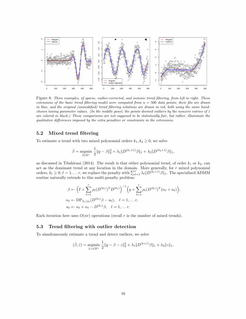
0 100 200 300 400 500

−2

−1

01

2 RegularSparse

●

●

●

●

●

●

●●●

●

●

●

●

●

●

●●

●●●

●●

●

●

●

●●

●

●

●

●

●

●

●

●

●●●

●●

●●

●●

●●

●

●

●

●

●

●

●

●

●

●

●

●

●

●

●

●

●

●

●

●

●

●

●

●

●

●

●

●

●

●

●●●

●●●

●

●

●

●

●

●

●●

●

●●

●

●

●

●

●

●

●●

●

●

●

●

●

●●

●

●

●●

●

●

●●●●

●

●●

●

●●●

●

●●

●

●

●

●

●

●

●

●

●●●

●

●

●

●

●

●

●

●

●

●●

●●●

●

●

●

●

●

●

●

●

●

●●

●

●

●

●

●

●

●

●

●

●●

●

●

●

●●

●

●

●

●

●

●

●

●

●

●

●

●

●

●

●●

●

●

●

●

●

●●

●

●

●

●●

●

●

●

●

●

●

●

●

●

●

●

●

●

●

●●

●

●

●

●

●●

●

●

●

●

●●

●

●

●

●

●●

●

●

●

●

●●●

●

●●

●●

●●

●

●●

●

●

●●

●

●

●

●

●

●

●

●

●

●

●

●

●

●

●

●

●

●

●

●

●●

●●

●

●

●

●

●●

●

●

●

●●

●●

●

●

●

●

●●

●

●

●

●

●

●

●●

●

●

●

●

●

●

●●

●

●

●●

●

●

●

●

●

●

●

●

●

●●

●●●

●

●

●

●

●

●

●

●

●

●●

●●

●

●

●

●

●

●

●

●

●

●●●

●●●

●

●

●

●

●

●

●

●●●●

●

●●

●

●

●

●

●

●

●

●

●

●

●

●

●

●

●

●

●

●●

●

●●●●●●

●

●●

●●

●●

●●

●

●

●

●

●

●

●

●

●

●

●●●

●

●

●

●

●

●

●

●

●

●

●

●

●

●

●

●

●

●

●

●

●

●●

●●

●

●

●

●

●

●

●

●

●

●●

●

●

●

●

●

●

●

●

●

●

●●

●

●

●

●

●●

●●

●

●

●

●

●

●

●

●

●

●

●

●

●

●

0 100 200 300 400 500

−1.

5−

1.0

−0.

50.

00.

51.

01.

5

●● ●●

●

RegularOutlier adjusted

●

●

●●

●

●

●

●●

●

●

●●

●●●

●

●

●

●

●

●●

●

●

●

●

●

●

●●●●●

●

●●

●

●

●

●

●

●●●●

●

●●

●

●

●

●

●

●●

●

●

●

●

●●

●

●

●

●

●

●●●●●

●

●

●

●

●●

●

●

●

●

●

●●●

●

●

●

●

●

●

●

●

●

●

●

●

●

●●

●●

●

●

●

●

●

●

●

●

●

●●

●

●

●

●●●●●

●●●

●●

●

●

●

●

●

●

●

●

●●●●●

●

●

●

●●●●

●

●

●

●

●

●

●

●

●

●

●

●

●

●

●

●

●

●●

●

●

●

●

●

●

●●●

●

●

●

●

●

●

●●

●

●

●●

●

●

●

●●

●

●

●

●

●

●

●●

●●

●

●●

●

●

●

●

●

●

●

●

●

●●

●

●

●

●

●

●

●

●

●

●

●

●

●

●

●

●●

●

●

●

●

●

●

●

●

●

●

●

●

●

●

●

●●

●

●●

●

●

●●

●

●

●●●

●

●

●

●

●

●

●

●

●

●

●

●

●

●

●

●

●

●

●

●

●●●

●

●

●

●●

●

●

●

●●

●

●

●●

●●

●

●

●

●

●

●

●●●

●

●●

●●

●

●

●

●

●

●

●●●

●

●

●

●

●

●

●●

●●

●

●

●●●

●

●

●

●●●

●

●●●

●

●

●

●

●

●

●

●

●

●

●

●

●●

●

●

●

●

●

●

●

●

●

●●

●

●

●

●●●

●

●●●

●●

●

●

●

●

●

●

●

●

●

●●

●

●●

●

●

●●

●

●

●

●

●

●

●

●

●

●

●

●

●

●

●

●

●

●

●●

●

●

●

●

●

●

●●

●

●

●

●

●

●

●

●

●

●●

●●

●

●

●

●

●

●

●

●

●

●

●

●

●

●

●

●

●

●

●

●

●

●

●

●

●●

●

●●

●●

●

●

●●

●

●

●

●

●

●

●

●

●

●

●

●

●●●

●●

●

●

●

0 100 200 300 400 500

−1

01

23

4

RegularIsotonic

Figure 8: Three examples, of sparse, outlier-corrected, and isotonic trend filtering, from left to right. Theseextensions of the basic trend filtering model were computed from n = 500 data points; their fits are drawnin blue, and the original (unmodified) trend filtering solutions are drawn in red, both using the same hand-chosen tuning parameter values. (In the middle panel, the points deemed outliers by the nonzero entries of zare colored in black.) These comparisons are not supposed to be statistically fair, but rather, illuminate thequalitative differences imposed by the extra penalties or constraints in the extensions.

5.2 Mixed trend filtering

To estimate a trend with two mixed polynomial orders k1, k2 ≥ 0, we solve

β = argminβ∈Rn

1

2‖y − β‖22 + λ1‖D(k1+1)β‖1 + λ2‖D(k2+1)β‖1,

as discussed in Tibshirani (2014). The result is that either polynomial trend, of order k1 or k2, canact as the dominant trend at any location in the domain. More generally, for r mixed polynomialorders, k` ≥ 0, ` = 1, . . . r, we replace the penalty with

∑r`=1 λ`‖D(k`+1)β‖1. The specialized ADMM

routine naturally extends to this multi-penalty problem:

β ←(I +

r∑`=1

ρ`(D(k`))TD(k`)

)−1(y +

r∑`=1

ρ`(D(k`))T (α` + u`)

),

α` ← DPλ`/ρ`(D(k`)β − u`), ` = 1, . . . r,

u` ← u` + α` −D(k`)β, ` = 1, . . . r.

Each iteration here uses O(nr) operations (recall r is the number of mixed trends).

5.3 Trend filtering with outlier detection

To simultaneously estimate a trend and detect outliers, we solve

(β, z) = argminβ,z∈Rn

1

2‖y − β − z‖22 + λ1‖D(k+1)β‖1 + λ2‖z‖1,

16

as in Kim et al. (2009), She & Owen (2011), where the nonzero components of z correspond toadaptively detected outliers. A short derivation leads to the updates:(

βz

)←(I + ρ1(D(k))TD(k) I

I (1 + ρ2)I

)−1(y + ρ1(D(k))T (α+ u)

y + ρ2(γ + v)

),

α← DPλ1/ρ1(D(k)β − u),

γ ← Sλ2/ρ2(z − v),

u← u+ α−D(k)β, v ← v + γ − z.

Again, this routine uses O(n) operations per iteration. See Figure 8 for an example.

5.4 Isotonic trend filtering

A monotonicity constraint in the estimated trend is straightforward to encode:

β = argminβ∈Rn

1

2‖y − β‖22 + λ‖D(k+1)β‖1 subject to β1 ≤ β2 ≤ . . . ≤ βn,

as suggested by Kim et al. (2009). The specialized ADMM updates are easy to derive:

β ←((1 + ρ2)I + ρ1(D(k))TD(k)

)−1(y + ρ1(D(k))T (α+ u) + ρ2(γ + v)

),

α← DPλ/ρ(D(k)β − u),

γ ← IR(β − v),

u← u+ α−D(k)β, v ← v + γ − β.

where IR(z) denotes an isotonic regression fit on z; since this takes O(n) time (e.g., Stout (2008)),a round of updates also takes O(n) time. Figure 8 gives an example.

5.5 Nearly-isotonic trend filtering

Instead of enforcing strict monotonicity in the fitted values, we can penalize the pointwise nonmon-tonicities with a separate penalty, following Tibshirani et al. (2011):

β = argminβ∈Rn

1

2‖y − β‖22 + λ1‖D(k+1)β‖1 + λ2

n−1∑i=1

(βi − βi+1)+.

This results in a “nearly-isotonic” fit β. Above, we use x+ = max{x, 0} to denote the positive partof x. The specialized ADMM updates are:

β ←((1 + ρ2)I + ρ1(D(k))TD(k)

)−1(y + ρ1(D(k))T (α+ u) + ρ2(γ + v)

),

α← DPλ1/ρ1(D(k)β − u),

γ ← DP+λ2/ρ2

(β − v),

u← u+ α−D(k)β, v ← v + γ − β.

where DP+t (z) denotes a nearly-isotonic regression fit to z, with penalty parameter t. It can be

computed in O(n) time by modifying the dynamic programming algorithm of Johnson (2013) forthe 1d fused lasso, so one round of updates still takes O(n) time.

17

6 Conclusion

We proposed a specialized but simple ADMM approach for trend filtering, leveraging the strength ofextremely fast, exact solvers for the special case k = 0 (the 1d fused lasso problem) in order to solvehigher order problems with k ≥ 1. The algorithm is fast and robust over a wide range of problemsizes and regimes of regularization parameters (unlike primal-dual interior point methods, the currentstate-of-the-art). Our specialized ADMM algorithm converges at a far superior rate to (accelerated)first-order methods, coordinate descent, and (what may be considered as) the standard ADMMapproach for trend filtering. Finally, a major strength of our proposed algorithm is that it can bemodified to solve many extensions of the basic trend filtering problem. Software for our specializedADMM algorithm is accessible through the trendfilter function in the R package glmgen, builtaround a lower level C package, both freely available at https://github.com/statsmaths/glmgen.

Acknowledgements. Taylor Arnold and Veeranjaneyulu Sadhanala contributed tremendouslyto the development of the new glmgen package. We thank the anonymous Associate Editor andReferees for their very helpful reading of our manuscript. This work was supported by NSF GrantDMS-1309174.

References

Arnold, T. & Tibshirani, R. J. (2014), Efficient implementations of the generalized lasso dual pathalgorithm. arXiv: 1405.3222.

Boyd, S., Parikh, N., Chu, E., Peleato, B. & Eckstein, J. (2011), ‘Distributed optimization andstatistical learning via the alternative direction method of multipliers’, Foundations and Trendsin Machine Learning 3(1), 1–122.

Boyd, S. & Vandenberghe, L. (2004), Convex Optimization, Cambridge University Press, Cambridge.

Davies, P. L. & Kovac, A. (2001), ‘Local extremes, runs, strings and multiresolution’, Annals ofStatistics 29(1), 1–65.

de Boor, C. (1978), A Practical Guide to Splines, Springer, New York.

Hastie, T. & Tibshirani, R. (1990), Generalized additive models, Chapman and Hall, London.

Johnson, N. (2013), ‘A dynamic programming algorithm for the fused lasso and L0-segmentation’,Journal of Computational and Graphical Statistics 22(2), 246–260.

Kim, S.-J., Koh, K., Boyd, S. & Gorinevsky, D. (2009), ‘`1 trend filtering’, SIAM Review 51(2), 339–360.

Mammen, E. & van de Geer, S. (1997), ‘Locally apadtive regression splines’, Annals of Statistics25(1), 387–413.

Rudin, L. I., Osher, S. & Faterni, E. (1992), ‘Nonlinear total variation based noise removal algo-rithms’, Physica D: Nonlinear Phenomena 60, 259–268.

She, Y. & Owen, A. B. (2011), ‘Outlier detection using nonconvex penalized regression’, Journal ofthe American Statistical Association: Theory and Methods 106(494), 626–639.

Steidl, G., Didas, S. & Neumann, J. (2006), ‘Splines in higher order TV regularization’, InternationalJournal of Computer Vision 70(3), 214–255.

18

Stout, Q. (2008), ‘Unimodal regression via prefix isotonic regression’, Computational Statistics andData Analysis 53(2), 289–297.

Tibshirani, R. J. (2014), ‘Adaptive piecewise polynomial estimation via trend filtering’, Annals ofStatistics 42(1), 285–323.

Tibshirani, R. J., Hoefling, H. & Tibshirani, R. (2011), ‘Nearly-isotonic regression’, Technometrics53(1), 54–61.

Tibshirani, R. J. & Taylor, J. (2011), ‘The solution path of the generalized lasso’, Annals of Statistics39(3), 1335–1371.

Tibshirani, R., Saunders, M., Rosset, S., Zhu, J. & Knight, K. (2005), ‘Sparsity and smoothness viathe fused lasso’, Journal of the Royal Statistical Society: Series B 67(1), 91–108.

Wahba, G. (1990), Spline Models for Observational Data, Society for Industrial and Applied Math-ematics, Philadelphia.

Wang, Y., Smola, A. & Tibshirani, R. J. (2014), ‘The falling factorial basis and its statisticalproperties’, International Conference on Machine Learning 31.

A Appendix: further details and simulations

A.1 Algorithm details for the motivating example

First, we examine in Figure 9 the condition numbers of the discrete difference operators D(k+1) ∈R(n−k−1)×n, for varying problem sizes n, and k = 0, 1, 2. Since the plot uses a log-log scale, thestraight lines indicate that the condition numbers grow polynomially with n (with a larger exponentfor larger k). The sheer size of the condition numbers (which can reach 1010 or larger, even fora moderate problem size of n = 5000) is worrisome from an optimization point of view; roughlyspeaking, we would expect the criterion in these cases to be very flat around its optimum.

●

●

●

●

●

100 200 500 1000 2000 5000

1e+

031e

+05

1e+

071e

+09

1e+

11

n

Con

ditio

n nu

mbe

r of

(k+

1)st

ope

rato

r

●

●

●

●

●

●

●

●

●

●

k=0k=1k=2

Figure 9: A log-log plot of the condition number of D(k+1) versus the problem size n, for k = 0, 1, 2,where the condition numbers scale roughly like nk.

19

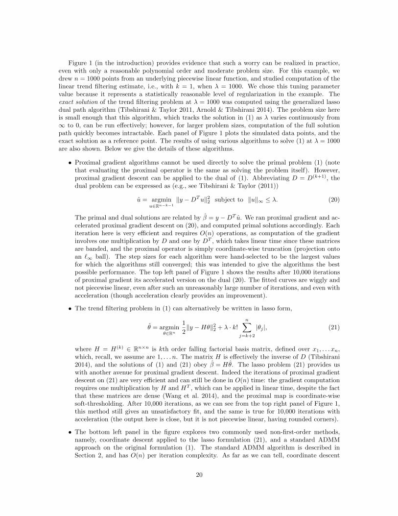
Figure 1 (in the introduction) provides evidence that such a worry can be realized in practice,even with only a reasonable polynomial order and moderate problem size. For this example, wedrew n = 1000 points from an underlying piecewise linear function, and studied computation of thelinear trend filtering estimate, i.e., with k = 1, when λ = 1000. We chose this tuning parametervalue because it represents a statistically reasonable level of regularization in the example. Theexact solution of the trend filtering problem at λ = 1000 was computed using the generalized lassodual path algorithm (Tibshirani & Taylor 2011, Arnold & Tibshirani 2014). The problem size hereis small enough that this algorithm, which tracks the solution in (1) as λ varies continuously from∞ to 0, can be run effectively; however, for larger problem sizes, computation of the full solutionpath quickly becomes intractable. Each panel of Figure 1 plots the simulated data points, and theexact solution as a reference point. The results of using various algorithms to solve (1) at λ = 1000are also shown. Below we give the details of these algorithms.

• Proximal gradient algorithms cannot be used directly to solve the primal problem (1) (notethat evaluating the proximal operator is the same as solving the problem itself). However,proximal gradient descent can be applied to the dual of (1). Abbreviating D = D(k+1), thedual problem can be expressed as (e.g., see Tibshirani & Taylor (2011))

u = argminu∈Rn−k−1

‖y −DTu‖22 subject to ‖u‖∞ ≤ λ. (20)

The primal and dual solutions are related by β = y −DT u. We ran proximal gradient and ac-celerated proximal gradient descent on (20), and computed primal solutions accordingly. Eachiteration here is very efficient and requires O(n) operations, as computation of the gradientinvolves one multiplication by D and one by DT , which takes linear time since these matricesare banded, and the proximal operator is simply coordinate-wise truncation (projection ontoan `∞ ball). The step sizes for each algorithm were hand-selected to be the largest valuesfor which the algorithms still converged; this was intended to give the algorithms the bestpossible performance. The top left panel of Figure 1 shows the results after 10,000 iterationsof proximal gradient its accelerated version on the dual (20). The fitted curves are wiggly andnot piecewise linear, even after such an unreasonably large number of iterations, and even withacceleration (though acceleration clearly provides an improvement).

• The trend filtering problem in (1) can alternatively be written in lasso form,

θ = argminθ∈Rn

1

2‖y −Hθ‖22 + λ · k!

n∑j=k+2

|θj |, (21)

where H = H(k) ∈ Rn×n is kth order falling factorial basis matrix, defined over x1, . . . xn,which, recall, we assume are 1, . . . n. The matrix H is effectively the inverse of D (Tibshirani2014), and the solutions of (1) and (21) obey β = Hθ. The lasso problem (21) provides uswith another avenue for proximal gradient descent. Indeed the iterations of proximal gradientdescent on (21) are very efficient and can still be done in O(n) time: the gradient computationrequires one multiplication by H and HT , which can be applied in linear time, despite the factthat these matrices are dense (Wang et al. 2014), and the proximal map is coordinate-wisesoft-thresholding. After 10,000 iterations, as we can see from the top right panel of Figure 1,this method still gives an unsatisfactory fit, and the same is true for 10,000 iterations withacceleration (the output here is close, but it is not piecewise linear, having rounded corners).

• The bottom left panel in the figure explores two commonly used non-first-order methods,namely, coordinate descent applied to the lasso formulation (21), and a standard ADMMapproach on the original formulation (1). The standard ADMM algorithm is described inSection 2, and has O(n) per iteration complexity. As far as we can tell, coordinate descent

20

requires O(n2) operations per iteration (one iteration being a full cycle of coordinate-wiseminimizations), because the update rules involve multiplication by individual columns of H,and not H in its entirety. The plot shows the results of these two algorithms after 5000iterations each. After such a large number of iterations, the standard ADMM result is fairlyclose to the exact solution in some parts of the domain, but overall fails to capture the piecewiselinear structure. Coordinate descent, on the other hand, is quite far off (although we note thatit does deliver a visually perfect piecewise linear fit after nearly 100,000 iterations).

• The bottom right panel in the figure justifies the perusal of this paper, and should generateexcitement in the curious reader. It illustrates that after just 20 iterations, both the PDIPmethod of Kim et al. (2009), and our special ADMM implementation deliver results that arevisually indistinguishable from the exact solution. In fact, after only 5 iterations, the special-ized ADMM fit (not shown) is visually passable. Both algorithms use O(n) operations periteration: the PDIP algorithm is actually applied to the dual problem (20), and its iterationsreduce to solving linear systems in the banded matrix D; the special ADMM algorithm indescribed in Section 2.

A.2 ADMM versus PDIP for k = 3 (piecewise cubic fitting)

For the case k = 3 (piecewise cubic fitting), the behavior of PDIP mirrors that in the k = 2 case,yet the convergence issues begin to show at problem sizes smaller by an order of magnitude. Thespecialized ADMM approach is slightly slower to converge, but overall still quite fast and robust.Figure 10 supports this point.

A.3 Prediction at arbitrary points

Continuing within the nonparametric regression context, an important task to consider is that offunction prediction at arbitrary locations in the domain. We discuss how to make such predictionsusing trend filtering. This topic is not directly relevant to our particular algorithmic proposal, butour R software package that implements this algorithm also features the function prediction task,and hence we describe it here for completeness. The trend filtering estimate, as defined in (1),produces fitted values β1, . . . βn at the given input points x1, . . . xn. We may think of these fittedvalues as the evaluations of an underlying fitted function f , as in

(f(x1), . . . f(xn)

)= (β1, . . . βn).

Tibshirani (2014), Wang et al. (2014) argue that the appropriate extension of f to the continuousdomain is given by

f(x) =

k+1∑j=1

φj · hj(x) +

n−k−1∑j=1

θj · hk+1+j(x), (22)

where h1, . . . hn are the falling factorial basis functions, defined as

hj(x) =

j−1∏`=1

(x− x`), j = 1, . . . k + 1,

hk+1+j(x) =

k∏`=1

(x− xj+`) · 1{x ≥ xj+k}, j = 1, . . . n− k − 1,

and φ ∈ Rk+1, θ ∈ Rn−k−1 are inverse coefficients to β. The first k + 1 coefficients index the poly-nomial functions h1, . . . hk+1, and defined by φ1 = β1, and

φj =1

(j − 1)!·[diag

(1

xj − x1, . . .

1

xn − xn−j+1

)·D(x,j−1)

]1

· β, j = 2, . . . k + 1. (23)

21

0 20 40 60 80 100

5e+

025e

+03

5e+

045e

+05

Iteration

Crit

erio

nPrimal−dual IPSpecial ADMM

0 20 40 60 80 100

5020

050

020

0010

000

5000

0

Iteration

Crit

erio

n

Primal−dual IPSpecial ADMM

0 20 40 60 80 100

5010

020

0

Iteration

Crit

erio

n

Primal−dual IPSpecial ADMM

0 50 100 150 200

1e+

031e

+05

1e+

071e

+09

1e+

11

Iteration

Crit

erio

n

Primal−dual IPSpecial ADMM

0 50 100 150 200

1e+

031e

+05

1e+

071e

+09

Iteration

Crit

erio

nPrimal−dual IPSpecial ADMM

0 50 100 150 200

500

1000

2000

5000

1000

0

Iteration

Crit

erio

n

Primal−dual IPSpecial ADMM

Figure 10: Convergence plots for (k = 3): achieved criterion values across iterations of ADMM and PDIP,with the same layout as in Figures 5a and 6a, except that the first row uses n = 1000 points, and the secondrow n = 10, 000 points. Both algorithms comfortably converge when n = 1000. However, PDIP encountersserious difficulties when n = 10, 000, reminiscent of its behavior for k = 2 but when n = 100, 000 (see Figure6a). In all cases, the specialized ADMM algorithm demonstrates a strong and steady convergence behavior.

Above, we use A1 to denote the first row of a matrix A. Note that φ1, . . . φk+1 are generally nonzeroat the trend filtering solution β. The last n− k − 1 coefficients index the knot-producing functionshk+2, . . . hn, and are defined by

θ = D(x,k+1)β/k!. (24)

Unlike φ, it is apparent that many of θ1, . . . θn−k−1 will be zero at the trend filtering solution, moreso for large λ. Given a trend filtering estimate β, we can precompute the coefficients φ, θ as in (23).Then, to produce evaluations of the underlying estimated function f at arbitrary points x′1, . . . x

′m,

we calculate the linear combinations of falling factorial basis functions according to (22). Fromthe precomputed coefficients φ, θ, this requires only O(mr) operations, where r = ‖D(x,k+1)β‖0, thenumber of nonzero (k + 1)st order differences at the solution (we are taking k to be a constant).

22