Fast and Efﬁcient Dynamic WDM Semiconductor … OF LIGHTWAVE TECHNOLOGY, VOL. 24, NO. 11, NOVEMBER...

JOURNAL OF LIGHTWAVE TECHNOLOGY, VOL. 24, NO. 11, NOVEMBER 2006 4353

Fast and Efficient Dynamic WDM SemiconductorOptical Amplifier Model

Walid Mathlouthi, Pascal Lemieux, Massimiliano Salsi, Armando Vannucci, Member, IEEE,Alberto Bononi, and Leslie A. Rusch, Senior Member, IEEE

Abstract—A novel state-variable model for semiconductoroptical amplifiers (SOAs) that is amenable to block diagramimplementation of wavelength division multiplexed (WDM) sig-nals and fast execution times is presented. The novel modelis called the reservoir model, in analogy with similar block-oriented models for Raman and erbium-doped fiber amplifiers(EDFAs). A procedure is proposed to extract the needed reservoirmodel parameters from the parameters of a detailed and accuratespace-resolved SOA model due to Connelly, which was extendedto cope with the time-resolved gain transient analysis. Severalvariations of the reservoir model are considered with increasingcomplexity, which allow the accurate inclusion of scattering lossesand gain saturation induced by amplified spontaneous emission.It is shown that at comparable accuracy, the reservoir modelcan be 20 times faster than the Connelly model in single-channeloperation; much more significant time savings are expected forWDM operation. The model neglects intraband SOA phenomenaand is thus limited to modulation rates per channel not exceeding10 Gb/s. The SOA reservoir model provides a unique tool withreasonably short computation times for a reliable analysis of gaintransients in WDM optical networks with complex topologies.

Index Terms—Optical pulse amplification, semiconductoroptical amplifier (SOA).

I. INTRODUCTION

S EMICONDUCTOR optical amplifiers (SOAs) are becom-ing key devices for future optical networks. SOAs are used

in a wealth of applications to achieve highly varied functions.For example, optical switching and wavelength conversioncan be accomplished using cross-gain modulation (XGM),four-wave mixing (FWM), or cross-phase modulation (XPM)[1]–[3]. Signal reshaping and noise cleaning of ON–OFF keying(OOK) signals are also feasible using saturated SOAs [4],with particularly effective application in spectrum slicedwavelength-division multiplexing (WDM) [5] and incoherentoptical code-division multiple access [6].

Manuscript received March 15, 2006; revised July 18, 2006. This work wassupported in part by FQRNT under Grant PADCO FT076892, the CanadianInstitute for Photonic Innovation under Grant CG082485, and the ItalianMinistry under Project WONDER.

W. Mathlouthi, P. Lemieux, and L. A. Rusch are with the Center of Optics,Photonics and Lasers, Département de Génie Électrique et Informatique, Uni-versité Laval, Ste-Foy, QC G1K 7P4, Canada (e-mail: [email protected];[email protected]; [email protected]).

M. Salsi, A. Vannucci, and A. Bononi are with the Dipartimento di Ingegne-ria dell’Informazione, Universitá di Parma, 43100 Parma, Italy (e-mail: [email protected]; [email protected]).

Color versions of Figs. 2–4, 6–9, and 11–16 are available online athttp://ieeexplore.ieee.org.

Digital Object Identifier 10.1109/JLT.2006.884217

In this paper, we are interested in analyzing the responseof SOAs to optical signals that are modulated at bit rates notexceeding 10 Gb/s, such as those planned for next-generationmetropolitan area networks. Therefore, ultrafast intraband phe-nomena such as carrier heating (CH) and spectral hole burning(SHB) (see, e.g., [7]–[9]) can be neglected, and only carrier-induced gain dynamics need to be included, as was donein several SOA models developed in the past. Such modelscan be divided into two broad categories: 1) space-resolvednumerically intensive models, which take into account facet re-flectivity as well as forward and backward propagating signalsand amplified spontaneous emission (ASE) and offer a goodfit to experimental data [10]–[12], and 2) simplified analyticalmodels with a coarser fit to experimental data but developed tofacilitate conceptual understanding and performance analysis[2], [13]–[16]. For the purpose of carrying out extensive MonteCarlo simulations for statistical signal analysis and bit-error-rate (BER) estimation, the accurate space-resolved models areruled out because of their prohibitively long simulation times.However, a simplified model with a satisfactory fit to experi-mental results would be highly desirable. Most simplified mod-els can be derived from the work of Agrawal and Olsson [13].Under suitable assumptions, Agrawal and Olsson managed toreduce the coupled propagation and rate equations into a singleordinary differential equation (ODE) for the integrated gain[13, eq. (3.4)]. The simplicity of the solution is due to the factthat waveguide scattering losses and ASE were neglected. ASEhas an important effect on the spatial distribution of carrierdensity and saturation, and it may significantly affect the SOAsteady-state and dynamic responses [17], [18]. Scattering lossesalso have an impact on the dynamic response of the SOA [3].Moreover, Agrawal and Olsson’s model was originally cast forsingle-wavelength-channel amplification, although it can be ex-tended to multiwavelength operation by assuming that the chan-nels are spaced far enough apart to neglect FWM beating in thecopropagating case [3]. Saleh [14] arrived independently at thesame model as Agrawal and Olsson’s ([14, eq. (4a)] coincideswith [13, eq. (3.4)]) and then introduced further simplifyingapproximations to get to a very simple block diagram of thesingle-channel SOA, which was exploited for a mathematicallyelegant stochastic performance analysis of single-channel sat-urated SOAs [15]. The loss of accuracy due to Saleh’s extraapproximations with respect to Agrawal’s model was quantifiedin [19]. Saleh’s model was later extended to cope with injectioncurrent modulation, scattering losses, and ASE [16]. In addi-tion, Agrawal’s model was extended to include ASE [20]. Inboth [16] and [20], ASE was added phenomenologically at the

0733-8724/$20.00 © 2006 IEEE

4354 JOURNAL OF LIGHTWAVE TECHNOLOGY, VOL. 24, NO. 11, NOVEMBER 2006

Fig. 1. Block diagram of the reservoir model. ASE contribution not shown forease of drawing.

output of the SOA and did not influence the gain dynamics,thereby limiting the application to very small saturation levels.

In this paper, we first develop a dynamic version of thesteady-state wideband SOA Connelly model [12], which isshown to fit quite well with our dynamic SOA experimentswith OOK channels. The Connelly model was selected becauseit derives the SOA material gain coefficient from quantummechanical principles without the assumption of linear de-pendence on carrier density that was made in [10] and [11].Our dynamic Connelly model serves then as a benchmark totest the accuracy and computational-speed improvement of anovel state-variable SOA dynamic model, which represents themost important contribution of this paper. The novel modelis an extension of Agrawal’s model, as provided in [3], withthe inclusion of approximations for scattering loss and ASEto better fit the experimental results and the dynamic Con-nelly model predictions. In such a model, the SOA dynamicbehavior is reduced to the solution of a single ODE for thesingle state variable of the system, which is proportional tothe integrated carrier density [3], which, for WDM operation,is a more appropriate variable than the integrated gain used in[13]. Once the state-variable dynamic behavior is found, thebehavior of all the output WDM channels is also obtained. Thestate variable is called “reservoir” since it plays the same roleas the reservoir of excited erbium ions in an erbium-dopedfiber amplifier (EDFA) [21], [22]. Quite interestingly, then,the SOA for WDM operation admits almost the same blockdiagram description as that of an EDFA suggested by [21,eq. (5)]. Such a novel SOA block diagram is shown in Fig. 1(without ASE for ease of drawing) and will be derived in thenext sections. Note that this model treats the intensity of theelectrical field, but the field phase can be indirectly obtainedsince it is a deterministic function of the reservoir [13]. In theSOA, the role of the optical pump for EDFAs is played bythe injected current I . The most striking difference betweenthe two kinds of amplifiers is the fluorescence time τ , whichis of the order of milliseconds in EDFAs and of a fractionof nanosecond in SOAs. Such a huge difference accounts formost of the disparity in the dynamic behavior between the twokinds of amplifiers and explains why SOAs have not been usedfor WDM applications for a long time [23]. However, recentcheap gain-clamped SOAs [24] are likely to promote the use ofSOAs for WDM metro applications. As already mentioned, thereservoir model requires the (copropagating) WDM channelsto have minimum channel spacing in excess of a few tens of

gigahertz, in order to neglect the carrier-induced FWM fieldsgenerated in the SOA. This should not be a problem for chan-nels allocated on the International Telecommunications Uniongrid with 50 GHz spacing or more. However, an intrinsic limitof the reservoir model is its neglecting SHB and CH, whichgenerate FWM and XPM interactions among WDM channelseven when the minimum channel spacing is large enough torule out any carrier-induced interaction [9]. The predictionsof the reservoir model will be accurate whenever the carrier-induced XGM mechanism dominates over FWM and XPM. It isworth mentioning that state-variable amplifier block diagramsare very important simulation tools that enable the reliablepower propagation of WDM signals in optical networks withcomplex topologies; therefore, the present reservoir SOA modelprovides a new entry aside from the already known models forEDFAs [21], [25] and for Raman amplifiers [26]. A challengein our reservoir model, as in all simplified SOA models, isto correctly choose the values of the wavelength-dependentcoefficients that give the best fit to the experimental results. Wepropose and describe here a methodology to extract the neededwavelength-dependent coefficients from the parameters of thedynamic Connelly model.

This paper is organized as follows. In Section II, the dynamicConnelly model is introduced, and a procedure to derive itsparameters from experiments is described. In Section III, theSOA reservoir model is derived first without ASE and thenwith ASE that is resolved over a large number of wavelengthbins. Simulations show good accordance between the reservoirmodel predictions and experiments, and good improvement incalculation time with respect to the Connelly model. However,inclusion of many ASE wavelength channels makes even thereservoir model too slow for the BER estimations we havein mind. Hence, in order to further simplify the model, weintroduce the reservoir model with a single equivalent ASEchannel. The ASE can be seen as an independent input-signalchannel (with proper input power and wavelength) that depletesthe reservoir of a noiseless SOA. Results show that this lastmodel is the most efficient one since it can be made to accu-rately predict experimental results with an execution time that is20 times faster than that of the dynamic Connelly model forsingle-channel operation, with the savings increasing with thenumber of WDM signal channels. In Section III-C, we examinea model that was obtained by dividing the SOA into severalsections, each characterized by its own reservoir. Here again,the ASE can be modeled as a single channel that propagatesthrough the different reservoir stages. Results show better pre-cision, although the increase in precision is not worth, in mostcases, the loss in execution time. Most of the numerical resultsare reported in Section IV. Finally, Section V summarizes themain findings of this paper.

II. DYNAMIC CONNELLY MODEL

A. Theory

In this paper, we adopt the wideband model for a bulk SOAproposed in [12], which is based on the numerical solutionof the coupled equations for carrier-density rate and photon-flux propagation for both the forward and backward signals

MATHLOUTHI et al.: FAST AND EFFICIENT DYNAMIC WDM SOA MODEL 4355

and the spectral components of ASE. At a specified time tand position z in the SOA, the propagation equation of photonflux Q±

k [photons/s] of the kth forward (+) or backward (−)signal is

dQ±k (z, t)dz

= {± [Γgk(N) − α(N)]}Q±k (z, t) (1)

where Γ is the fundamental mode confinement factor, gk is thematerial gain coefficient at the optical frequency νk of the kthsignal, α is the material-loss coefficient, and both are functionsof carrier density N(z, t). The power of the propagating signalis related to its photon flux as P±

k = hνkQ±k (in watts), where h

is Planck’s constant. The ASE photon flux on each ASE wave-length channel obeys a similar propagation equation given by

dQ±j (z, t)dz

= ± [Γgj(N) − α(N)]Q±j (z, t) +Rsp,j(N) (2)

where Rsp,j(N) is the spontaneous emission rate coupled intothe ASE channel at frequency νj . The expression of Rsp,j(N)is given in [12, eq. (40)]. This expression will be used inSection III-B to develop a reservoir model equation that takesASE into account. The carrier density at coordinate z evolvesas [12]

dN(z, t)dt

=I

qdLW−R (N(z, t))

− ΓdW

{nsig∑k=1

gk(N)(Q+

k (z, t) +Q−k (z, t)

)}

− 2ΓdW

nASE∑j=1

gj(N)Kj

(Q+

j (z, t) +Q−j (z, t)

)(3)

where I is the bias current; q is the electron charge; d, L, and Ware the active-region thickness, length, and width, respectively,and R(N) is the recombination rate. An expression for R(N)is given in [12, eq. (49)]; the reservoir model of Section III usesa linear approximation for R(N) in (9); nsig is the number ofWDM signals; nASE is the number of spectral components ofthe ASE; and Kj is an ASE multiplying factor, which equals1 for zero facet reflectivity [12]. The factor 2 in (3) accountsfor two ASE polarizations. Note that (3) contains an importantapproximation: it is the sum of the signals and ASE powers(fluxes), instead of—more correctly—the power of the sumof the signals and ASE fields, that depletes carrier density N .Therefore, (3) neglects the carrier-density pulsations due tobeating among WDM channels that generate FWM and XPMin SOAs [9]. Although such an approximation is inappropriatefor extremely dense or high-power WDM channels, it isaccurate for typical wavelength spacings of 0.4 nm or more.

The material gain gk(N) ≡ g(νk, N) is calculated as in[12, eq. (14)]. Fig. 2 plots the material gain N versus wave-length λk = c/νk (with c being the speed of light) using theSOA parameters discussed in the next section.

Fig. 2. Gain coefficient g(λ, N) versus wavelength and carrier density calcu-lated from ([12, eq. (14)]) with the parameters in Table I.

The time-varying solution of the coupled differential equa-tions (1)–(3) is based on the assumption that the carrier densityremains constant during a time step and is achieved by firstperforming a spatial integration with the carrier density fixedduring each time step, followed by a time integration. Steady-state solutions are used as an initial condition for the subsequenttime evolution.

We note in closing that the Connelly model also neglectsultrafast phenomena such as CH and SHB.

B. Parametrization

In order to fit the experimental results that we obtained with acommercial Optospeed SOA model 1550MRI X1500, we usedthe SOA parameters provided in [12, Table I], except for asubset of different values reported in Table I in this paper; themost critical of such parameters were determined as follows.

1) The active-region length L was determined by measuringthe frequency spacing between two maxima of the gainspectrum ripples: L = λ2

0/2nr∆λ, where λ0 is the cen-tral wavelength (1550 nm), nr is the average semicon-ductor refractive index, and ∆λ is the ripple wavelengthspacing.

2) The bandgap energy Eg0 was set so that the experimentalcutoff wavelength of the gain spectrum (which was about1605 nm) matched the simulated one.

3) The parameters of the carrier-dependent material-losscoefficient [12], i.e.,

α (N(z)) = K0 + ΓK1N (4)

were chosen so that the maximum simulated gainmatched the measured one.

4) The active-region thickness and width were set so as tomatch the experimental and simulated curves of gain as afunction of the injection current.


TABLE IVALUES OF PARAMETERS USED IN THE CONNELLY MODEL, WHICH DIFFER FROM THOSE IN [12]

Fig. 3. Fiber to fiber unsaturated gain versus wavelength. Measured (dashed)and simulation (solid) results using Connelly model.

5) The bandgap shrinkage coefficient Kg was set so thatthe peak gain wavelength equals the measured value of1560 nm at an injection current of 500 mA.

The aforementioned SOA parameter values were used in allsimulations hereafter.

C. Simulations With Connelly Model

We present simulation results obtained with the Connellymodel and compare them against experimental measurements.The experiment consisted in amplifying a tunable continuouswave (CW) laser whose wavelength was varied around theOptospeed SOA peak gain wavelength. Laser polarization wascontrolled so as to obtain maximum gain.1) Unsaturated Gain Spectrum: Fig. 3 shows the simulated

and measured unsaturated gain spectra at a signal input powerof −30 dBm and an injection current of 500 mA.

A good match between the simulations and experiments wasobtained when using the values of Table I. In the ensuing

Fig. 4. Fiber to fiber gain versus input optical power. Measured (dashed) andConnelly model (solid).

experiments and simulations, the input signal will be fixed atthe gain peak wavelength of 1560 nm.2) Gain Saturation: Fig. 4 shows the fiber-to-fiber gain as a

function of the input power. The wavelength of the input laserwas 1560 nm, and the injection current was 500 mA.3) Dynamic Response: The experimental setup is depicted

in Fig. 5. The input laser at 1560 nm was externally modulatedat 1 Gb/s. The laser power was varied from −25 to −10 dBmin steps of 5 dB. The measured photoreceiver responsivity was400 mV/mW. The injection current was 500 mA. Since we areinterested in testing the action of the SOA on the propagatingsignal power in this paper, no optical filter was inserted beforedetection.1

1The phase response of optical filters can vary nonlinearly with frequency.Signals not precisely centered in the filter passband have the chirp acquiredwithin the SOA transformed into an undesired amplitude modulation, leadingto unpredictable pulse shapes that mask the SOA gain dynamics.


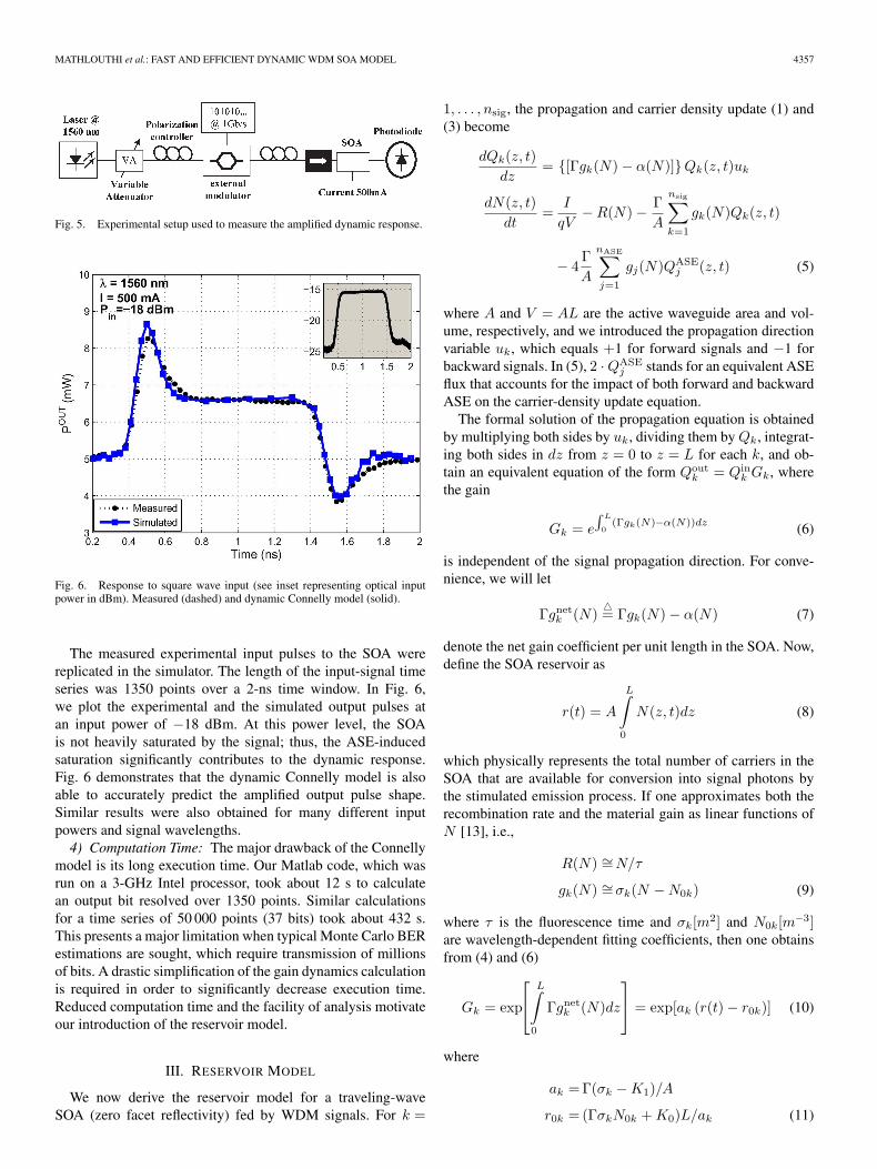
Fig. 5. Experimental setup used to measure the amplified dynamic response.

Fig. 6. Response to square wave input (see inset representing optical inputpower in dBm). Measured (dashed) and dynamic Connelly model (solid).

The measured experimental input pulses to the SOA werereplicated in the simulator. The length of the input-signal timeseries was 1350 points over a 2-ns time window. In Fig. 6,we plot the experimental and the simulated output pulses atan input power of −18 dBm. At this power level, the SOAis not heavily saturated by the signal; thus, the ASE-inducedsaturation significantly contributes to the dynamic response.Fig. 6 demonstrates that the dynamic Connelly model is alsoable to accurately predict the amplified output pulse shape.Similar results were also obtained for many different inputpowers and signal wavelengths.4) Computation Time: The major drawback of the Connelly

model is its long execution time. Our Matlab code, which wasrun on a 3-GHz Intel processor, took about 12 s to calculatean output bit resolved over 1350 points. Similar calculationsfor a time series of 50 000 points (37 bits) took about 432 s.This presents a major limitation when typical Monte Carlo BERestimations are sought, which require transmission of millionsof bits. A drastic simplification of the gain dynamics calculationis required in order to significantly decrease execution time.Reduced computation time and the facility of analysis motivateour introduction of the reservoir model.

III. RESERVOIR MODEL

We now derive the reservoir model for a traveling-waveSOA (zero facet reflectivity) fed by WDM signals. For k =

1, . . . , nsig, the propagation and carrier density update (1) and(3) become

dQk(z, t)dz

= {[Γgk(N) − α(N)]}Qk(z, t)uk

dN(z, t)dt

=I

qV−R(N) − Γ

A

nsig∑k=1

gk(N)Qk(z, t)

− 4ΓA

nASE∑j=1

gj(N)QASEj (z, t) (5)

where A and V = AL are the active waveguide area and vol-ume, respectively, and we introduced the propagation directionvariable uk, which equals +1 for forward signals and −1 forbackward signals. In (5), 2 ·QASE

j stands for an equivalent ASEflux that accounts for the impact of both forward and backwardASE on the carrier-density update equation.

The formal solution of the propagation equation is obtainedby multiplying both sides by uk, dividing them by Qk, integrat-ing both sides in dz from z = 0 to z = L for each k, and ob-tain an equivalent equation of the form Qout

k = Qink Gk, where

the gain

Gk = e

∫ L

0(Γgk(N)−α(N))dz (6)

is independent of the signal propagation direction. For conve-nience, we will let

Γgnetk (N)

�= Γgk(N) − α(N) (7)

denote the net gain coefficient per unit length in the SOA. Now,define the SOA reservoir as

r(t) = A

L∫0

N(z, t)dz (8)

which physically represents the total number of carriers in theSOA that are available for conversion into signal photons bythe stimulated emission process. If one approximates both therecombination rate and the material gain as linear functions ofN [13], i.e.,

R(N) ∼=N/τ

gk(N) ∼=σk(N −N0k) (9)

where τ is the fluorescence time and σk[m2] and N0k[m−3]are wavelength-dependent fitting coefficients, then one obtainsfrom (4) and (6)

Gk = exp

L∫

0

Γgnetk (N)dz

= exp[ak (r(t) − r0k)] (10)

where

ak = Γ(σk −K1)/A

r0k = (ΓσkN0k +K0)L/ak (11)


are two dimensionless parameters. In addition, one can multiplyboth sides of the second equation in (5) by A and integrate indz to obtain

dr(t)dt

=I

q− r(t)

τ−

nsig∑k=1

L∫0

Γgk (N(z))Qk(z) dz

− 4nASE∑j=1

L∫0

Γgj (N(z))QASEj (z) dz. (12)

For the time being, the contribution of ASE will be neglected.It will be tackled in Section III-B. Now, integrating in dz bothsides of the first equation in (5) gives

L∫0

Γgk(N)Qk dz =(Qout

k −Qink

)+

L∫0

α(N)Qk dz. (13)

The Appendix discusses the approximation involved in drop-ping the second term on the right-hand side of (13), whichphysically represents the signal photons lost through scatteringwithin the SOA. If such a scattering loss term can be dropped,then substituting in (12), one gets the “reservoir dynamic equa-tion” given by

dr(t)dt

=I

q− r(t)

τ−

nsig∑k=1

Qink

(eak(r(t)−r0k) − 1

)(14)

where gain Gk (10) takes the scattering losses into account.Since the scattering loss term is positive, the reservoir result-ing from (14) is an overestimation of the actual reservoir, asquantified in the Appendix.

Note that the reservoir dynamic equation is quite similar tothe EDFA reservoir equation [21] and, together with gain (10),builds the block diagram shown in Fig. 1.

As discussed in [13], one can easily show that once reservoirr(t) is known, the cumulated phase of the kth propagatingsignal at the output of the SOA can be obtained as

φoutk (t) = −1

2αH

Γσk

A(r(t) −N0kV ) (15)

where αH is the “linewidth enhancement factor.” Therefore,it is possible to correctly take into account chirp-related dis-tortions that are induced by dispersive optical components thatfollow the SOA.

A. Extraction of Reservoir Parameters From Connelly Model

We next explain how to extract the fitting parameters of thegain linearization in (9) from the Connelly gain g(λ,N), whoseplot versus wavelength and carrier density was already given inFig. 2 for our Optospeed SOA. A plot of gnet

k (λ,N) would havea similar form; in particular, a rigid shift downward would resultif K1 = 0, i.e., if α did not depend on N .

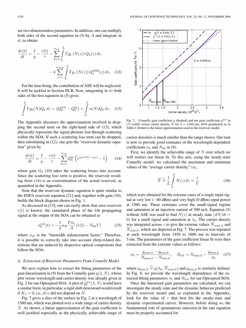
Fig. 7 gives a slice of the surface in Fig. 2 at a wavelength of1560 nm, which was plotted over a wide range of carrier densityN . As shown, a linear approximation of the gain coefficient iswell justified especially as the physically achievable range of

Fig. 7. Connelly gain coefficient g (dashed) and net gain coefficient gnet in(7) (solid) versus carrier density N for λ = 1560 nm. SOA parameters as inTable I. Dotted is the linear approximation used in the reservoir model.

carrier densities is much smaller than the range shown. Our taskis now to provide good estimates of the wavelength-dependentcoefficients σk and N0k in (9).

First, we identify the achievable range of N over which wewill restrict our linear fit. To this aim, using the steady-stateConnelly model, we calculated the maximum and minimumvalues of the “average carrier density,” i.e.,

N�=

1L

L∫0

N(z) dz =r

V(16)

which were obtained for the extreme cases of a single input sig-nal at very low (−40 dBm) and very high (0 dBm) input powerat 1560 nm. These extremes cover the small-signal regimeand saturation at an injection current of 500 mA. Equation (5)without ASE was used to find N(z) at steady state (dN/dt =0) for a small signal and saturation at λk. The carrier densitywas integrated across z to give the extreme values Nmax,k andNmin,k, which are depicted in Fig. 7. The process was repeatedat each wavelength from 1450 to 1600 nm in intervals of5 nm. The parameters of the gain coefficient linear fit were thenextracted from the extreme values as follows:

σk =gmax,k − gmin,k

Nmax,k −Nmin,k, N0,k = Nmax,k − gmax,k

σk(17)

where gmax,k�= g(λk, Nmax,k) and gmin,k is similarly defined.

In Fig. 8, we provide the wavelength dependence of the ex-tracted fitting parameters σk and N0,k for our Optospeed SOA.

Once the linearized gain parameters are calculated, we caninvestigate the steady state and the dynamic behavior predictedby the reservoir model and, as explained in the Appendix,look for the value of τ that best fits the steady-state anddynamic experimental curves. However, before doing so, thefundamental role of spontaneous emission in the rate equationmust be properly accounted for.


Fig. 8. Coefficients σk (squares solid) and N0,k (triangle solid) of thelinearization of the gain coefficient g versus wavelength for our OptospeedSOA. Also shown are the coefficients γk and N1,k of the linearization of theemission gain coefficient g′ (see Section III-B).

B. Including ASE

We now take into account the ASE-induced saturation termin (5) that was neglected in the previous section. The ASE fluxat z is obtained by solving the propagation (2) with zero initialcondition [27]:

QASEj (z) = Gj(z)

z∫0

Rsp,j (N(s))Gj(s)

ds (18)

where Gj(z) = exp[∫ z

0 Γgnetj (N(z′))dz′] is the gain from 0

to z. If, for this calculation, we assume that the carrier density isconstant along z at the average carrier density N = r/V , thenthe preceding equation simplifies to

QASEj (z) ∼= Rsp,j(N)

Γgnetj (N)

(eΓgnet

j (N)z − 1). (19)

Such an expression can now be used to evaluate the ASEintegrals neglected in (12) in the previous section, i.e.,

L∫0

Γgj(N)QASEj (z) dz ∼= gj(N)

gnetj (N)

· Rsp,j(N)Γgnet

j (N)

· (G(r) − 1 − lnG(r)) (20)

where G(r) = exp{Γgnetj (N)L} is the gain and is a function of

the reservoir only. Note that the fraction gj/gnetj on the right-

hand side of (20) also appeared in the treatment of the signalsin the Appendix. It approaches one when the scattering-losscoefficient is small compared with the gain coefficient, and inthe following, it will be considered equal to one in the sameway we dealt with the signals in the previous section.

The fraction in (19) represents the spontaneous emissionfactor nsp,j at the jth wavelength of the SOA multiplied bythe resolution bandwidth of the ASE channels ∆νASE. Con-nelly [12, eq. (40)] points out that Rsp,j(N) = Γg′j(N)∆νASE,where g′j > gj is the emission gain coefficient [12, eq. (16)],

which may significantly differ from the gain coefficient gj

at shorter wavelengths. If we linearize g′j(N) ∼= γj(N −N1j)and use the linearization (9) of gj , then we get

nsp,j =Rsp,j(N)/∆νASE

Γgnetj (N)

∼= Γγj(r − r1j)Aaj(r − r0j)

(21)

where r1j�= N1jV . As a dimensional check, γj and A are

measured in [m2], while aj is dimensionless so as to correctlyobtain a dimensionless nsp,j .

Fig. 8 also shows the values of the wavelength-dependentcoefficients γj and N1j in the linearization of g′, which wereobtained using exactly the same procedure that yields thelinearization coefficients of g detailed in Section III-A.

Finally, using (12), (20), and (21), the reservoir dynamicequation including ASE becomes

dr(t)dt

=I

q− r(t)

τ−

nsig∑k=1

Qink

(eak(r(t)−r0k) − 1

)

− 4∆νASE

nASE∑j=1

nsp,j(r) (Gj(r) − 1 − lnGj(r)) . (22)

It is worth noting that a similar equation is found for the caseof EDFAs in [29, eq. (13)]. The received ASE flux QASE

j (L),finally, is calculated from (19) and (21).

Since this equation still partly neglects some contributions ofthe effect of scattering loss, as discussed in the Appendix, wefound it convenient to tune the value of the fluorescence timeτ in the reservoir model so as to best match the dynamic andstatic behaviors of the Optospeed SOA used in the experiments.A value close to τ = 310 ps was found to give an excellent fitin the cases that we analyzed.

As a first example of the validity of (22), we calculatedboth with the Connelly model and with the reservoir modelthe total received ASE power when a single nonreturn-to-zero modulated channel at 1560 nm, with a 0101 modulatingsequence at 1 Gb/s, was fed to the SOA with an input powerof −18 dBm. Fig. 9 shows the total received ASE power as afunction of time for both models, with a satisfactory agreement.Extensive comparisons will be presented in Section IV.

C. Multistage Reservoir Model

The multistage reservoir model consists of subdividingthe SOA into several cascaded sections or “stages,” eachcharacterized by its own reservoir (Fig. 10). Let ns be thenumber of stages. Then, the reservoir equation for eachstage i is

dri

dt=I

q− ri

τ−

nsig∑k=1

Qink,i(Gk(ri)−1)−

nASE∑j=1

QASE,inj,i (Gj(ri)−1)

− 4∆νASE

nASE∑j=1

nsp,j(ri) (Gj(ri) − 1 − ln (Gj(ri))) (23)

where ri is the reservoir of the ith stage with length Li = L/ns

and Gk(ri) is its gain given in (10) and (11) (where Li is


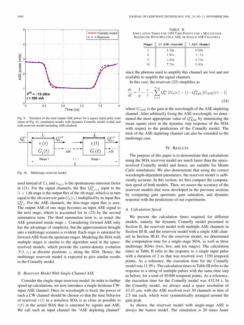
Fig. 9. Variation of the total output ASE power for a square input pulse train(inset of Fig. 6); simulation results with dynamic Connelly model (solid) andwith reservoir model including ASE (dashed).

Fig. 10. Multistage reservoir model.

used instead of L), and nsp,j is the spontaneous emission factorin (21). For the signal channels, the flux Qin

k,i+1 input to the(i+ 1)th stage is the output flux of the ith stage, which is in turnequal to the ith reservoir gainGk(ri) multiplied by its input fluxQin

k,i. For the ASE channels, the first-stage input flux is zero.The output ASE of one stage becomes an input ASE signal tothe next stage, which is accounted for in (23) by the secondsummation term. The third summation term is, as usual, theASE generated inside stage i. Considering forward ASE onlyhas the advantage of simplicity, but the approximation broughtinto a multistage scenario is evident: Each stage is saturated byforward ASE from the upstream stages. Modeling the SOA withmultiple stages is similar to the algorithm used in the space-resolved models, which provide the carrier-density evolutionN(t, zi) at discrete positions zi along the SOA. Hence, themultistage reservoir model is expected to give similar resultsto the Connelly model.

D. Reservoir Model With Single-Channel ASE

Consider the single-stage reservoir model. In order to furtherspeed up calculations, we now introduce a single fictitious CW-input ASE channel. Once its wavelength is fixed, the power ofsuch a CW channel should be chosen so that the time behaviorof reservoir r(t) in a noiseless SOA is as close as possible tor(t) in the actual SOA that is saturated by signals and ASE.We call such an input channel the “ASE depleting channel”

TABLE IISIMULATION TIMES FOR 1350 TIME POINTS FOR A MULTISTAGE

RESERVOIR WITH MULTIPLE ASE OR SINGLE ASE CHANNELS

since the photons used to amplify this channel are lost and notavailable to amplify the signal channels.

In this case, the reservoir (22) simplifies as

dr

dt=

I

q− r

τ−

nsig∑k=1

Qink (Gk(r) − 1)−Qin

ASE [GASE(r) − 1]

(24)

where GASE is the gain at the wavelength of the ASE depletingchannel. After arbitrarily fixing the ASE wavelength, we deter-mined the most appropriate value of Qin

ASE by minimizing themean square error in the dynamic step response of the SOAwith respect to the predictions of the Connelly model. Thetrick of the ASE depleting channel can also be extended to themultistage case.

IV. RESULTS

The purpose of this paper is to demonstrate that calculationsusing the SOA reservoir model are much faster than the space-resolved Connelly model and hence, are suitable for MonteCarlo simulations. We also demonstrate that using the correctwavelength-dependent parameters, the reservoir model is suffi-ciently accurate. In this section, we first compare the computa-tion speed of both models. Then, we assess the accuracy of thereservoir models that were developed in the previous sectionsby comparing gain spectrum, gain saturation, and dynamicresponse with the predictions of our experiments.

A. Calculation Speed

We present the calculation times required for differentmodels, namely, the dynamic Connelly model presented inSection II, the reservoir model with multiple ASE channels inSection III-B, and the reservoir model with a single ASE chan-nel in Section III-D. For the reservoir model, we determinedthe computation time for a single-stage SOA, as well as threemultistage SOAs (two, five, and ten stages). The calculationtimes in Table II refer to the response to a single input pulsewith a duration of 2 ns that was resolved over 1350 temporalpoints. As a reference, the execution time for the Connellymodel was 11.95 s. The calculation times in Table III refer to theresponse to a string of multiple pulses with the same time stepas before, for a total of 50 000 temporal points. As a reference,the execution time for the Connelly model was 432.54 s. Inthe Connelly model, we always used a space resolution of43.33 µm, with the ASE resolved over 30 channels in bins of2.5 nm each, which were symmetrically arranged around thegain peak.

As shown, the reservoir model with single-stage ASE isalways the fastest model. The simulation is 20 times faster


TABLE IIISIMULATION TIMES FOR 50 000 TIME POINTS FOR A MULTISTAGE

RESERVOIR WITH MULTIPLE ASE OR SINGLE ASE CHANNELS

Fig. 11. Fiber to fiber gain spectrum versus wavelength. Measured (dashed)and simulation (solid) results using the single (squares) and five-stage (circles)reservoir with 20 ASE channels.

than the Connelly model when a single ASE channel is used.However, when several reservoir stages are used, the calculationspeed of the single-ASE model becomes of the same order asthat of the multiple-ASE case. In this case, the use of multipleASE channels is better for accuracy.

The improvement in computation time in all reservoir modelswith respect to the Connelly model is predicted to significantlyincrease when increasing the number of propagated WDMsignal channels.

B. Single-Stage Reservoir With ASE

1) Gain Spectrum: Fig. 11 shows both simulated (solidlines with markers) and experimental fiber-to-fiber (dashed-dotted line) gain versus wavelength. The input laser power was−25 dBm. We can see a reasonable match between simula-tions and experiments. A slight gap between simulation andexperiment is observed at shorter wavelengths. The peak gainwavelength was the same in both simulations and experiment.We also see that the five-stage reservoir model is slightly moreaccurate than the single-stage reservoir one.2) Gain Saturation: Fig. 12 shows both simulated and ex-

perimental fiber-to-fiber gains versus input power at a signalwavelength of 1560 nm. We see that the simulations reasonablypredict the small-signal gain. A slight discrepancy is observedwhen saturation sets in. This is attributed to the fact that theratio gk/g

netk is larger than one in deep saturation since the

denominator tends to zero. In such cases, it is preferable toinclude the term gk(r)/gnet

k (r) in the reservoir equation rather

Fig. 12. Fiber to fiber gain versus input optical power. Measured (dashed)and simulation (solid) results using the single (squares) and five-stage (circles)reservoir with 20 ASE channels.

Fig. 13. Response to square wave input. Measured (dashed) and simulation(solid) results using the single (squares) and five-stage (circles) reservoir with20 ASE channels.

than set it to 1 and play with the fitting parameter τ , as we didin this paper. Here again, we see that the five-stage reservoir iscloser to the experimental data.3) Dynamic Response: Fig. 13 shows the simulated (solid

with squared markers) and experimental (dashed) response inmilliwatts to a square-wave input (see inset in Fig. 6). Sim-ulations include the ASE total detected power, which plays afundamental role in the reservoir equation, since it partiallysaturates the amplifier, hence reducing the amplifier gain. Wesee that the CW levels (zero and one levels) are well predictedin Fig. 13. This suggests that the approximation that we usedto calculate the ASE power is valid, although the simulated andexperimental output pulses are slightly different. We see thatthe pulse’s overshoot and undershoot are better predicted by thefive-stage reservoir model.


Fig. 14. Fiber to fiber gain versus optical input power. Measured (dashed) andsimulated (solid) results using a three-stage reservoir with single channel ASE.

C. Multistage Reservoir With ASE

Figs. 11–13 show the gain spectrum, gain saturation at1560 nm, and the output pulse power for the five-stage (solidwith circle markers) reservoir with ASE, respectively. The para-meters used in the simulations are the same as those consideredin the single-stage reservoir model. Increasing the stage numberbeyond five does not increase the accuracy, which might beattributed to the neglect of ASE that propagates backwardacross the stages. In these figures, we see that the dynamicand steady-state fits are more accurate than those in the singlestage. Particularly, the simulated gain spectrum shape (Fig. 11)is closer to the experimental one compared with the single-stagereservoir. Moreover, the overshoot and undershoot of the outputpulse are much closer to the experimental one. However, thisprecision comes at the price of simulation speed: The larger thenumber of stages, the longer the execution time (see Tables IIand III). An advantage of the multistage model is that it allowstrading execution time for precision, eventually reaching acomparable precision (and a comparable computational burden)as the space-resolved Connelly model.

D. Multistage Reservoir With ASE Depleting Channel

In order to fit the experimental results, we arbitrarily fixedthe ASE-depleting-channel wavelength at 1520 nm and thenfound the value of its input flux, which gave the minimum meansquare error fit with the prediction of the Connelly model.

As shown in Figs. 14 and 15, the simulation results arenot far from the experimental ones, but they are less accuratethan those in the multichannel ASE case. To investigate thedynamic response, we cascaded three reservoir stages andpropagated both the signal and the ASE depleting channel.We note from the figures that simulations fit measurementsin a way comparable to the multistage reservoir with ASE,which proves the effectiveness of the ASE-depleting-channelapproach. Moreover, the advantage of this approach is thecomputation speed. In fact, ASE-depleting-channel simulations

Fig. 15. Response to a square wave input. Measured (dashed) and simulated(solid) results using a three-stage reservoir with ASE depleting channel.

are twice as fast as those for the multichannel ASE case (seeTables II and III). The use of more than three stages does notimprove accuracy.

E. WDM Amplification

In order to verify the efficiency of our model for a widerrange of simulation scenarios, we investigated the case ofWDM-signal amplification. We recall that both the Connellyand the reservoir models are not able to reproduce carrier-induced nonlinear effects such as FWM and XPM and canonly model the effects of carrier-induced self-gain modulationand XGM.

Fig. 16 shows the measured power at the output of our Op-tospeed SOA as well as simulation results using the Connellymodel and (a) a one-stage reservoir model and (b) a three-stagemodel, in which the fluorescence τ was set at the value of360 ps to best match the measurements. The SOA was fedwith four synchronously OOK-modulated WDM signals witha wavelength spacing of 3 nm (λ1 = 1550 nm, λ2 = 1553 nm,λ3 = 1556 nm, and λ4 = 1559 nm). The SOA output isoptically filtered so that the ASE is eliminated, and the desiredchannel is selected. The optical filter is 1.2 nm wide, so its effecton the pulse shape is negligible at an experimental bit rate of1 Gb/s. The average input power of each channel is −20 dBm(experimentally, lower input power showed noisy pulses).Under such conditions, we observe a good match betweenthe measurements and the Connelly model predictions. Areasonable match is also obtained between the experimentand the reservoir models. However, we verified that atlower input powers, the simulations give a less exact fit.The lack of accuracy during the transients is due to thelinear approximations of the gain and recombination rate.Note the different slopes of measured and simulated pulsesafter the overshoot in Fig. 15. We believe the reason forthis to lie in the linear approximation of R(N) is when thesignal reaches a maximum (and the carrier density reaches


Fig. 16. Response of four WDM channels (with a spacing of 3 nm) to a squarewave input (see inset showing input optical powers in dBm). (a) Measured(dashed) and dynamic Connelly model (solid). (b) Measured (dashed), one-stage reservoir with single channel ASE (solid with squares) and three-stagereservoir with single channel ASE(solid with circles).

a minimum), the actual time constant of the SOA is largerthan that employed in (9). Moreover, ultrafast phenomena(neglected in this paper) will have an increasing impactfor overshoots and undershoots on the order of a fewpicoseconds.

V. CONCLUSION

A novel state-variable SOA model that is amenable to blockdiagram implementation for WDM applications and with fast

execution times was presented and discussed. We called thenovel model the reservoir model, in analogy with similar block-oriented models for EDFAs and Raman amplifiers. While ASEself-saturation can be simply included in the EDFA reservoirmodel [28], an added complexity in SOAs with respect toEDFAs is that scattering losses cannot be neglected. This in-creases the difficulty in developing a reservoir model for SOAs,and we proposed innovative solutions to tackle the problem.A critical step in the SOA reservoir model is the appropriateselection of the values of its wavelength-dependent parametersthat provide a good fit with the experiments. We proposed anddescribed at length a procedure to extract such parameters fromthe parameters of a detailed and accurate space-resolved SOAmodel due to Connelly, which we extended to cope with thetime-resolved gain transient analysis. It is important to notethat our reservoir model is not entirely dependent on the space-resolved simulator. The key wavelength-dependent parameterfor the reservoir model is the material gain as a function ofboth wavelength and inversion. A detailed knowledge of thisdependence allows accurate linearization around the workingpoint and hence, more accuracy for the reservoir model. Aprocedure to extract the model parameters directly from themeasurements would be of great practical value.

A number of other issues remain to be explored and deservefurther research. The presence of nonzero facet reflectivity wasnot considered and would be important for modeling reflectiveSOAs with the reservoir. In addition, a different approximationfor the recombination rate, accounting for a reservoir-dependenttime constant, could increase the reliability of the model. In thispaper, we assumed a linear dependence of this parameter onthe inversion. A better approximation (R(r) = a1(r) + a2r

2 +a3r

3 + . . .) could be obtained if we assume a constant inversionN = r/V over the SOA length (as we did for ASE calculationsin Section III-B). However, the accuracy obtained with suchapproximations will be at the cost of slower execution time.

The raison d’être of the reservoir model is to find a tradeoffbetween accuracy and calculation speed. To achieve this goal,we considered several variations of the model, with increasingcomplexity, which allow the accurate inclusion of both scat-tering losses and gain saturation induced by ASE. To speedup the emulation of transmission of long bit sequences in thereservoir model, we introduced a single equivalent input ASEchannel with appropriate power and gain parameters, whichfeeds a noiseless reservoir model to give equivalent dynamics.We showed that at a comparable accuracy, the reservoir modelwith the single ASE channel can be 20 times faster than theConnelly model in single-channel operation, and much moresignificant time savings are expected for WDM operation. Theaccuracy of the model is limited to modulation rates per channelnot exceeding 10 Gb/s since ultrafast phenomena such as CHand SHB are neglected. However, such rates are of interestfor next-generation metropolitan optical networks. In addition,beating-induced carrier gratings that generate FWM and XPMin SOAs are not captured by the reservoir model, which thenis reliable whenever XGM dominates over such effects. Thetrue value of the SOA reservoir model is that together withblock diagram descriptions of EDFA and Raman amplifiers, itprovides a unique tool with reasonably short computation times


for reliable analysis of gain transients in WDM optical networkswith complex topologies.

APPENDIX

RESERVOIR EQUATION EXTENDED TO

SCATTERING LOSSES

In this Appendix, we take into account the scattering lossterm that was neglected in (13) in the derivation of the reservoirdynamic (14) in order to assess the approximation that weintroduced. If one assumes the carrier density along the SOAequals its average value N = r/V (16), then

Qk(z) ∼= Qink e

(Γgk(N)−α(N))z

and the term neglected in (13) can be approximated as

L∫0

α(N)Qkdz ∼= α(N)Qink

e(Γgk(N)−α(N))L − 1Γgk(N) − α(N)

.

Since (Γgk(N) − α(N))L = ak(r − r0k), we obtain the “ex-tended reservoir equation with scattering losses” as

dr(t)dt

=I

q− r(t)

τ−

nsig∑k=1

Qink

(eak(r(t)−r0k) − 1

)

×(

1 +α(

rV

)Γgk

(rV

)− α(

rV

)).

Since we can write

1 +α(N)

Γgk(N) − α(N)=

gk(N)gnet

k (N)

it is now evident that the reservoir (14) is accurate whenevergnet

k (N) ∼= gk(N). However, this is not always guaranteed tohold, especially for deeply saturated SOAs, as one can seefor instance in Fig. 7. While in principle one can solve thepreceding extended reservoir equation, in this paper, we found iteasier to solve the standard reservoir (14) and look for the valueof the fluorescence time τ that gave the best fit to both staticand dynamic measurements. In essence, a slightly “decreased”value of τ has the effect of extra depletion of the reservoir,which has the same qualitative effect of the extra depletioncaused by the neglected scattering loss term. Although it is clearthat the carrier lifetime has a conceptually different impact onsteady-state and transient responses, we chose, by numericaloptimization, the value of τ that leads to the best fit of themeasured gain spectrum to that predicted by the steady-stateConnelly model. We also show that it is possible to achieve anaccurate estimation of the step response at the same time.

ACKNOWLEDGMENT

A. Bononi would like to thank Dr. Y. Sun for the earlydiscussions about the existence of a reservoir model for SOAs.

REFERENCES

[1] T. Durhuus, B. Mikkelsen, C. Joergensen, S. L. Danielsen, andK. E. Stubkjaer, “All-optical wavelength conversion by semiconductoroptical amplifiers,” J. Lightw. Technol., vol. 14, no. 6, pp. 942–954,Jun. 1996.

[2] K. Obermann, S. Kindt, D. Breuer, and K. Petermann, “Performanceanalysis of wavelength converters based on cross-gain modulation insemiconductor optical amplifiers,” J. Lightw. Technol., vol. 16, no. 1,pp. 78–85, Jan. 1998.

[3] D. Marcenac and A. Mecozzi, “Switches and frequency converters basedon cross-gain modulation in semiconductor laser amplifiers,” IEEE Pho-ton. Technol. Lett., vol. 9, no. 6, pp. 749–751, Jun. 1997.

[4] F. Öhman, S. Bishoff, B. Tromborg, and J. Mørk, “Noise and regenerationin semiconductor waveguides with saturable gain and absorption,” IEEEJ. Quantum Electron., vol. 40, no. 3, pp. 245–255, Mar. 2004.

[5] M. Zhao, G. Morthier, and R. Baets, “Analysis and optimization of inten-sity noise reduction in spectrum-sliced WDM systems using a saturatedsemiconductor optical amplifier,” IEEE Photon. Technol. Lett., vol. 14,no. 3, pp. 390–392, Mar. 2002.

[6] M. Menif, W. Mathlouthi, P. Lemieux, L. A. Rusch, and M. Roy, “Error-free transmission for incoherent broadband optical communications sys-tems using incoherent-to-coherent wavelength conversion,” J. Lightw.Technol., vol. 23, no. 1, pp. 287–294, Jan. 2005.

[7] A. Uskov, J. Mork, and J. Mark, “Theory of short-pulse gain saturationin semiconductor laser amplifiers,” IEEE Photon. Technol. Lett., vol. 4,no. 5, pp. 443–446, May 1992.

[8] J. Mork and A. Mecozzi, “Theory of the ultrafast response of activesemiconductor waveguides,” J. Opt. Soc. Amer. B, Opt. Phys., vol. 13,no. 8, pp. 1803–1816, Aug. 1996.

[9] A. Mecozzi, S. Scotti, A. D’Ottavi, E. Iannone, and P. Spano, “Four-wavemixing in traveling-wave semiconductor amplifiers,” IEEE J. QuantumElectron., vol. 31, no. 4, pp. 689–699, Apr. 1995.

[10] D. Marcuse, “Computer model of an injection laser amplifier,” IEEE J.Quantum Electron., vol. QE-19, no. 1, pp. 63–73, Jan. 1983.

[11] T. Durhuus, B. Mikkelsen, and K. E. Stubkjaer, “Detailed dynamic modelfor semiconductor optical amplifiers and their crosstalk and intermodula-tion distortion,” J. Lightw. Technol., vol. 10, no. 8, pp. 1056–1065, Aug.1992.

[12] M. J. Connelly, “Wideband semiconductor optical amplifier steady-state numerical model,” IEEE J. Quantum Electron., vol. 37, no. 3,pp. 439–447, Mar. 2001.

[13] G. P. Agrawal and N. A. Olsson, “Self phase modulation and spectralbroadening of optical pulses in semiconductor laser amplifier,” IEEEJ. Quantum Electron., vol. 25, no. 11, pp. 2297–2306, Nov. 1989.

[14] A. A. M. Saleh, “Non linear models of travelling wave optical amplifiers,”Electron. Lett., vol. 24, no. 14, pp. 835–837, Jul. 1988.

[15] A. A. M. Saleh and I. M. I. Habbab, “Effects of semiconductor opti-cal amplifier nonlinearity on the performance of high-speed intensity-modulation lightwave systems,” IEEE Trans. Commun., vol. 38, no. 6,pp. 839–846, Jun. 1990.

[16] C. Tai and W. I. Way, “Dynamic range and switching speed limitations ofan N × N optical packet switch based on low-gain semiconductor opticalamplifiers,” J. Lightw. Technol., vol. 14, no. 4, pp. 962–967, Apr. 1992.

[17] T. Liu, K. Obermann, K. Petermann, F. Girardin, and G. Guekos, “Effectof saturation caused by amplified spontaneous emission on semicon-ductor optical amplifier performance,” Electron. Lett., vol. 33, no. 24,pp. 2042–2043, Nov. 1997.

[18] G. Talli and M. J. Adams, “Gain dynamics of semiconductor opticalamplifiers and three-wavelength devices,” IEEE J. Quantum Electron.,vol. 39, no. 10, pp. 1305–1313, Oct. 2003.

[19] M. M. Freire and H. J. A da Silva, “Performance implications of par-tial chirp compensation in a semiconductor optical booster amplifier fordispersion supported transmission at 10 Gb/s,” in Proc. ICT, Jun. 1998,vol. 1, pp. 76–80.

[20] M. Settembre, F. Matera, V. Hägele, I. Gabitov, A. W. Mattheus, andS. K. Turitsyn, “Cascaded optical communication systems with in-linesemiconductor optical amplifier,” J. Lightw. Technol., vol. 15, no. 6,pp. 962–967, Jun. 1997.

[21] A. Bononi and L. A. Rusch, “Doped-fiber amplifier dynamics: A systemperspective,” J. Lightw. Technol., vol. 16, no. 5, pp. 945–956, May 1998.


[22] Y. Sun, J. L. Zyskind, and A. K. Srivastava, “Average inversion level,modeling, and physics of erbium-doped fiber amplifiers,” IEEE J. Sel.Topics Quantum Electron., vol. 3, no. 4, pp. 991–1007, Aug. 1997.

[23] R. Ramaswami and P. A. Humblet, “Amplifier induced crosstalk inmultichannel optical networks,” J. Lightw. Technol., vol. 8, no. 12,pp. 1882–1896, Dec. 1990.

[24] E. Tangdiongga, J. J. J. Crijns, L. H. Spiekman, G. N. Van den Hoven,and H. de Waardt, “Performance analysis of linear optical amplifiers indynamic WDM systems,” IEEE Photon. Technol. Lett., vol. 14, no. 8,pp. 1196–1198, Aug. 2002.

[25] S. Novak and A. Moesle, “Simulink model for EDFA dynamics appliedto gain modulation,” J. Lightw. Technol., vol. 20, no. 6, pp. 986–992,Jun. 2002.

[26] A. Bononi, M. Papararo, and M. Fuochi, “Transient gain dynamicsin saturated Raman amplifiers,” Opt. Fiber Technol., vol. 10, no. 1,pp. 91–123, Jan. 2004.

[27] E. Kreyszig, Advanced Engineering Mathematics, 7th ed. New York:Wiley, 1993.

[28] L. Tancevski, A. Bononi, and L. A. Rusch, “Output power and SNRswings in cascades of EDFAs for circuit- and packet-switched op-tical networks,” J. Lightw. Technol., vol. 17, no. 5, pp. 733–742,May 1999.

[29] A. A. Rieznik and H. L. Fragnito, “Analytical solution for the dynamicbehavior of erbium-doped fiber amplifiers with constant population inver-sion along the fiber,” J. Opt. Soc. Amer. B, Opt. Phys., vol. 21, no. 10,pp. 1732–1739, Oct. 2004.

Walid Mathlouthi received the B.S.E.E. degreefrom École Nationale d’Ingénieurs de Tunis, Tunis,Tunisia, and the M.S.E.E degree from UniversitéLaval, Québec City, QC, Canada. He is currentlyworking toward the Ph.D. degree in electrical en-gineering at the Center of Optics, Photonics andLasers, Département de Génie Électrique et Informa-tique, Université Laval.

His research interests include semiconductor opti-cal amplifiers, spectrum-sliced wavelength-divisionmultiplexing, fiber Bragg gratings, optical code-

division multiple access, and wireless optical communications.

Pascal Lemieux received the B.S. degree (with hon-ors) in engineering physics from Université Laval,Québec City, QC, Canada, in 2004. He is currentlyworking toward the M.S. degree in optical telecom-munications at the Centre d’Optique, Photonique etLaser, Département de Génie Électrique et Informa-tique, Université Laval.

His research interests include semiconductor opti-cal amplifiers, spectrum-sliced wavelength-divisionmultiplexing, statistical properties of optical lightsources, optical code-division multiple access, andwireless optical communications.

Massimiliano Salsi was born in Parma, Italy, in1979. He received the Laurea degree (cum laude) intelecommunications engineering from the Universityof Parma, Parma, in 2004. He is currently workingtoward the Ph.D. degree in information technologyat the Department of Information Engineering, Uni-versity of Parma.

His current research interests include saturation,stabilization, and nonlinear effects in optical ampli-fiers for wavelength-division-multiplexing long-hauland metropolitan-networks applications.

Armando Vannucci (S’95–M’01) was born inFrosinone, Italy, in 1968. He received the Laureadegree (cum laude) in electronics engineering fromthe University of Roma “La Sapienza,” Rome, Italy,and the Ph.D. degree in information engineeringfrom the University of Parma, Parma, Italy, in 1993and 1998, respectively.

Until 1995, he was with the INFO-COM Depart-ment, University of Roma. Since 1995, he has beenwith the Department of Information Engineering,University of Parma, where he is currently an As-

sistant Professor of telecommunications. His current research interests includeoptical communication systems and polarization mode dispersion, nonlinearwavelength-division-multiplexing fiber transmission, system performance eval-uation, and optical amplifiers.

Alberto Bononi received the Laurea degree (cumlaude) in electronics engineering from the Univer-sity of Pisa, Pisa, Italy, in 1988 and the M.A.and Ph.D. degrees in electrical engineering fromPrinceton University, Princeton, NJ, in 1992, and1994, respectively.

He is currently an Associate Professor of telecom-munications with the Department of InformationEngineering, School of Engineering, University ofParma, Parma, Italy, where he teaches courses inprobability theory and stochastic processes, telecom-

munications networks, and optical communications. In 1990, he was withGEC-Marconi Hirst Research Centre, Wembley, U.K., where he worked on aMarconi S.p.A. project on coherent optical systems. From 1994 to 1996, hewas an Assistant Professor with the Department of Electrical and ComputerEngineering, State University of New York, Buffalo, where he taught courses inelectric circuits and optical networks. In summers 1997 and 1999, he was a Vis-iting Faculty with the Département de Genie Électrique, Université Laval, QC,Canada, where he did research on fiber amplifiers. His current research interestsinclude system design and performance analysis of high-speed all-opticalnetworks, nonlinear fiber transmission for wavelength-division-multiplexingsystems, linear and nonlinear polarization mode dispersion, and transient gaindynamics in optical amplifiers.

Leslie A. Rusch (S’91–M’94–SM’00) received theB.S.E.E. degree (with honors) from California In-stitute of Technology, Pasadena, in 1980 and theM.A. and Ph.D. degrees in electrical engineeringfrom Princeton University, Princeton, NJ, in 1992and 1994, respectively.

From 2001 to 2002, she was with Intel Corpora-tion as the Manager of a group that researches newwireless technologies. She is currently a Full Profes-sor with the Department of Electrical and ComputerEngineering, Université Laval, Québec City, QC,

Canada, performing research in wireless and optical communications. Herresearch interests include optical code-division multiple access using nonco-herent sources for metropolitan area networks, semiconductor and erbium-doped optical amplifiers and their dynamics, and wireless-communicationshigh-performance reduced-complexity receivers for ultrawideband systemsemploying code-division multiple access.

Fast and Efﬁcient Dynamic WDM Semiconductor … OF LIGHTWAVE TECHNOLOGY, VOL. 24, NO. 11, NOVEMBER...

Documents

Transcript of Fast and Efﬁcient Dynamic WDM Semiconductor … OF LIGHTWAVE TECHNOLOGY, VOL. 24, NO. 11, NOVEMBER...