Fast and accurate localization of multiple RF … · Fast and accurate localization of multiple RF...

RESEARCH ARTICLE

Fast and accurate localization of multiple RF markersfor tracking in MRI-guided interventions

Francesca Galassi • Djordje Brujic • Marc Rea •

Nicholas Lambert • Nandita Desouza • Mihailo Ristic

Received: 24 July 2013 / Revised: 7 April 2014 / Accepted: 7 April 2014 / Published online: 7 May 2014

� The Author(s) 2014. This article is published with open access at Springerlink.com

Abstract

Object A new method for 3D localization of N fiducial

markers from 1D projections is presented and analysed. It

applies to semi-active markers and active markers using a

single receiver channel.

Materials and methods The novel algorithm computes

candidate points using peaks in three optimally selected

projections and removes fictitious points by verifying detec-

ted peaks in additional projections. Computational com-

plexity was significantly reduced by avoiding cluster

analysis, while higher accuracy was achieved by using opti-

mal projections and by applying Gaussian interpolation in

peak detection. Computational time, accuracy and robustness

were analysed through Monte Carlo simulations and experi-

ments. The method was employed in a prototype MRI guided

prostate biopsy system and used in preclinical experiments.

Results The computational time for 6 markers was better

than 2 ms, an improvement of up to 100 times, compared

to the method by Flask et al. (J Magn Reson Imaging

14(5):617–627, 2001). Experimental maximum localiza-

tion error was lower than 0.3 mm; standard deviation was

0.06 mm. Targeting error was about 1 mm. Tracking

update rate was about 10 Hz.

Conclusion The proposed method is particularly suitable in

systems requiring any of the following: high frame rate,

tracking of three or more markers, data filtering or interleaving.

Keywords Magnetic resonance imaging � Tracking �MRI-guided intervention � 1D projections � RF markers

Introduction

Magnetic resonance imaging is increasingly being applied

to perform interventional procedures such as biopsies, laser

induced interstitial thermotherapy, high-intensity focused

ultrasound and endoscopy [2–8]. In many procedures it is

essential to be able to track the position of a device within

the imaging volume of the scanner and to communicate this

information in the form of an image feedback to the

interventional staff. As the instrument is not visible in the

MR image, fiducial markers mounted on the instrument are

often used for its localization. Fast and robust localization

of the fiducial markers is very important as it enables

higher frame update rate that, in turn, makes imaging more

consistent and, as such, improves hand–eye coordination.

In this manner the errors introduced by the movement of

both the patient and the interventional device are reduced

[9]. Importantly, more accurate and faster targeting enables

faster interventional procedures and decreases the cost of

intervention [10].

Fiducial markers may be classified as active, semi-active

or passive, each involving different localization techniques

[11–14]. An active fiducial marker is a microcoil receiver,

which provides the MR signal to a dedicated channel of the

MRI system [11]. As the received signal is highly local-

ized, this has the advantage of avoiding problems due to

background noise. Multiple markers may be easily distin-

guished if each is assigned to a dedicated receive channel.

A semi-active marker may be constructed as a resonant

microcircuit, which is inductively coupled to a receiver coil

of the MRI system [15]. Finally, a passive marker consists

of an encapsulated volume of material chosen to provide

good contrast in the acquired slices.

Both active and semi-active markers may be localized

using 1D projections, by determining the location of the

F. Galassi (&) � D. Brujic � M. Rea � N. Lambert �N. Desouza � M. Ristic

Mechanical Engineering Department, Imperial College London,

London, UK

e-mail: [email protected]

123

Magn Reson Mater Phy (2015) 28:33–48

DOI 10.1007/s10334-014-0446-3

signal peak, while passive markers demand the use of

image processing techniques, for example, template

matching [13]. The use of 1D projections lends itself to

much faster high-resolution data acquisition and processing

than image processing of multiple slices [1]. Flask et al. [1]

proposed a method for tracking N semi-active markers in

3D using 1D projections in two orthogonal planes and

cluster analysis. Their algorithm requires at least five 1D

projections per plane. However, projections with less than

N peaks are rejected, so new projections are acquired

instead. This results in an acquisition time of about 170 ms.

We propose a novel method for fast and accurate locali-

zation of N markers using 1D projections [16]. The method

may be applied to localize either semi-active markers or

active ones when only one receiver channel is used. By using

more than three markers, higher accuracy in localizing an

instrument may be achieved with no compromise in the

update rate. The complexity of the post-processing algorithm

was significantly reduced by avoiding cluster analysis [1],

while high accuracy was achieved by using optimal projec-

tions to compute the points and by applying Gaussian

interpolation in peak detection. The algorithm does not reject

projections with coincident peaks, resulting in reduced

scanning time, while the number of projections may be tra-

ded against robustness and accuracy, for optimized results in

a specific situation. Performance has been characterized

through a combination of extensive experimental studies and

Monte Carlo simulations. The experiments involved wire-

less markers, a customized GRE sequence, and an MR-

compatible moving platform. Preclinical volunteer studies

were conducted to verify the method under patient loading

and in the presence of physiological movements.

The proposed localization method was implemented

within a custom made system for image guided prostate

biopsy [17]. The application that integrates the tracking

algorithm with a novel visualization method, specific for

prostate biopsy, was implemented using Matlab and runs on a

dedicated navigation workstation located in the control room

and connected to the scanner via a local area network. The

image reconstruction pipeline was programmed to stream 1D

projections from the scanner to the navigation workstation just

after the Inverse Fourier Transformation has been completed.

Materials and methods

Algorithm for localizing N markers from multiple 1D

projections

Problem statement

The N markers generate N or fewer peaks along a 1D

projection. The problem is to compute the 3D coordinates

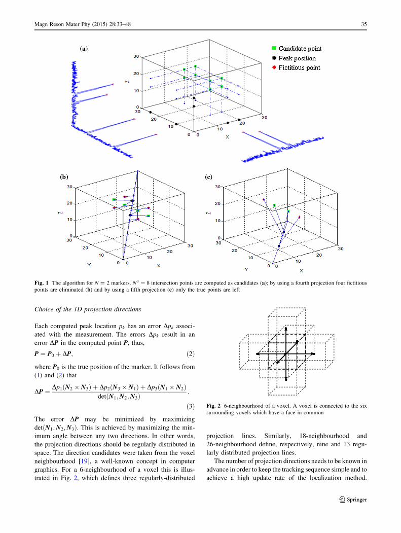
of N markers by using n 1D-projections. Each detected

peak defines a plane perpendicular to the corresponding

projection direction. In general, three 1D projections of

N points define three N planes which intersect at

N3 points. As a result N3 – N points are fictitious and

must be discarded. This can be done by using addi-

tional projections (Fig. 1). Each candidate marker posi-

tion is defined by the intersection of three planes,

whose normals are not co-planar and intersect at a point

P [18]:

P ¼ p1 N2 � N3ð Þ þ p2 N3 � N1ð Þ þ p3 N1 � N2ð Þdet N1;N2;N3ð Þ ; ð1Þ

where Nk (k = 1, 2, 3) is the unit vector of the direction of

a projection and pk is the position of the peak along this

direction.

Tracking algorithm

The method for tracking N markers consists of a number of

steps, which are summarized below and further details are

provided in the subsequent sections.

1. The process starts with the acquisition of a predefined

set of 1D projections, involving excitation of the whole

imaging volume. The number and directions of these

1D projections have been optimized, as presented

below.

2. Peak detection is performed for each projection, the

position of each peak is then determined with sub-pixel

resolution.

Three reference projections are selected, as explained

below, and N3 candidate marker positions are calculated

(Fig. 1a). The remaining projections are sorted according

to the decreasing minimal distance between the peaks they

contain. Projections with fewer than N peaks are placed at

the bottom of the list and used last. In this way projections

that may lose a peak have lower probability of being used

and affecting the result. Note that projections with a

smaller number of peaks, due to peak merging, will not

eliminate any of the correct points.

The fictitious (N3 – N) candidates are eliminated by

using, in turn, the remaining test projections. For each test

projection, the projected value of the each candidate point

is calculated and the distances between this and the iden-

tified peak locations are computed (Fig. 1b, c). The can-

didate is removed if the projected point does not have an

identified peak in its vicinity, i.e., if the minimum com-

puted distance is larger than an experimentally determined

tolerance e. If the number of computed points is different

from the known number of markers, then the entire solution

is discarded.

34 Magn Reson Mater Phy (2015) 28:33–48

123

Choice of the 1D projection directions

Each computed peak location pk has an error Dpk associ-

ated with the measurement. The errors Dpk result in an

error DP in the computed point P, thus,

P ¼ P0 þ DP; ð2Þ

where P0 is the true position of the marker. It follows from

(1) and (2) that

DP ¼ Dp1 N2 � N3ð Þ þ Dp2 N3 � N1ð Þ þ Dp3 N1 � N2ð Þdet N1;N2;N3ð Þ :

ð3Þ

The error DP may be minimized by maximizing

det N1;N2;N3ð Þ. This is achieved by maximizing the min-

imum angle between any two directions. In other words,

the projection directions should be regularly distributed in

space. The direction candidates were taken from the voxel

neighbourhood [19], a well-known concept in computer

graphics. For a 6-neighbourhood of a voxel this is illus-

trated in Fig. 2, which defines three regularly-distributed

projection lines. Similarly, 18-neighbourhood and

26-neighbourhood define, respectively, nine and 13 regu-

larly distributed projection lines.

The number of projection directions needs to be known in

advance in order to keep the tracking sequence simple and to

achieve a high update rate of the localization method.

Fig. 1 The algorithm for N = 2 markers. N3 ¼ 8 intersection points are computed as candidates (a); by using a fourth projection four fictitious

points are eliminated (b) and by using a fifth projection (c) only the true points are left

Fig. 2 6-neighbourhood of a voxel. A voxel is connected to the six

surrounding voxels which have a face in common

Magn Reson Mater Phy (2015) 28:33–48 35

123

Simulations were used in order to test the performance of the

algorithm in relation to the number of projections. As a

result, 13 projections were acquired and their directions

defined in accordance with the 26-neighbourhood.

Selection of the reference projections

Following the acquisition, peak detection and peak locali-

zation, three reference projections need to be selected from

the acquired set. For the case of 13 acquired projections

there are 13!= 13� 3ð Þ!3! ¼ 286 subsets of three directions

Ni;Nj;Nk. The subsets are ordered according to the

decreasing value of the determinant det N1;N2;N3ð Þ: The

first subset with N distinct peaks and a minimum distance

between two peaks greater than a prescribed value d is

selected as the reference subset. The latter condition

ensures that the candidate points are well distributed in the

volume so that the corresponding computed projected

values are well distributed along a projection direction,

which improves the success rate in the subsequent removal

of fictitious points.

Fiducial markers and tracking sequence

Fiducial markers

Fiducial markers were constructed similarly to [20], con-

sisting of 3 mm diameter wireless micro-coils tuned to the

Larmor frequency of the scanner and filled with high 1H

density, water-gel material (vinyl plastisol gel, Spenco

Healthcare, Horsham, UK) (Fig. 3).

A Vector Network Analyzer (Anritsu MS 2026A VNA

Master) was used to fine tune the RF marker to fr ¼123:5 MHz by using inductively coupled test coils

connected to the reflection and the transmission channel,

respectively. By measuring the bandwidth Df at -3 dB

between lower and upper cut-off frequency, the quality

factor was calculated as fr=Df .

Tracking sequence

A 2D spoiled GRE sequence was modified in order to

acquire a predefined set of 1D-projections, each projection

including a dephasing gradient to spoil the transverse

component of the magnetization prior to the next acquisi-

tion. The following parameters were made adjustable from

the user interface of the MR host computer: (1) flip-angle,

(2) magnitude of the dephaser gradient and (3) time

interval between individual projections. Other relevant

sequence parameters were TR = 5.6 ms, TE = 3.5 ms,

FOV 300 mm, 320 phase encode points.

Safety assessment

The potential local heating due to electromagnetic coupling

to the RF transmitter is an important issue to be considered

when using RF semi-active markers in the clinical envi-

ronment [21]. In order to verify the thermal safety of the

markers, an optic fibre thermometer (Luxtron 812, Luma-

Sense) with the accuracy of 0.1 �C was used. Similarly to

[21], the optic fibre sensor was taped directly onto a marker

which was, in turn, placed on top of a large water phantom.

The test was performed in a 1.5T MR Siemens scanner.

The temperature was recorded over 11 min, with no RF

excitation during the first minute (base line) and RF exci-

tation present during the subsequent 10 min. The test was

performed for a T2-weighted turbo spin echo (TSE)

sequence (whole body specific absorption rate

SAR = 0.7 W/kg), which is the imaging sequence rou-

tinely used in prostate imaging, and for the developed

tracking sequence (SAR \ 0.001 W/kg). The SAR values

were reported by the scanner. In both experiments the body

loading was represented by two 2 l phantoms placed

adjacently near the scanner’s isocentre. TSE imaging

sequence parameters (TR = 3,670, TE = 121 ms, flip

angle = 137�, slice thickness 3 mm, distance factor 10 %,

base resolution 320, phase resolution 70 %, turbo fac-

tor = 23) were set according to the protocol for prostate

imaging at Royal Marsden Hospital (Sutton, London, UK).

Signal analysis

Signal amplitude under repeated excitation

The micro-coil locally amplifies the excitation field. For an

applied flip angle aapp it results in an effective flip angle

Fig. 3 Wireless RF markers. Circuit (a) and marker (b), tuned to the

frequency (123.5 ± 0.05) MHz. The marker comprises two non-

magnetic capacitors and a 3 mm diameter inductor, filled with water–

gel (relaxation times T1 = 160 ms and T2 = 14 ms) and soldered on

two copper tape strips. The inductor was sealed with glue to avoid

contamination of the water–gel and for mechanical rigidity


123

aeff ¼ Q� aapp; where Q is the Q-factor of the micro-coil

[15]. With TR� T1, the magnetisation is expected to

approach the steady state over a set of projections [22]. The

aim is to maximize the amplitude of the received MR

signal for each projection, therefore to maximize the

transverse magnetization component at the echo time TE.

Similarly to Hargreaves et al. [23], the magnetization

vector was derived as:

MTE ¼ AMi þ B; ð4Þ

where Mi is the magnetization vector just before the RF

pulse, A and B are matrices representing the RF nutation

about the x-axis, the precession about z-axis and the T1 and

T2 relaxation processes. The transverse component

MTEXYwas then computed as MTEXY

¼ffiffiffiffiffiffiffiffiffiffiffiffiffiffiffiffiffiffiffiffiffiffiffiffiffiffiffi

M2TEXþM2

TEY

q

and

simulated (T1 = 160 ms, T2 = 14 ms, TE = 3.5 ms,

TR = 5.6 ms) for a marker under repeated excitation and

for flip angles 0:1�\aapp\0:5�. The flip angle aapp, which

gives higher amplitude of the received signal, was thus

estimated. Experimentally, 1D projections were acquired in

the presence of the large water phantoms.

Marker orientation to the main magnetic field

Orientation of the marker to the main field is an important

factor to be considered when designing interventional

devices [15]. At some angles the amplitude of the signal

might be comparable with the background signal and;

hence, peak detection may become unreliable. This was

investigated experimentally using a custom made rotary

holder to position the marker’s axis at various known

angles to the main field. The induced RF flux is dependent

on the angle between the axis of the coil and B1 field. The

signal is in turn dependent on induced RF flux and its

orientation with respect to the main field. These depen-

dencies tend to reduce the signal as the coil axis rotates

from B1 to B0. In our experiment a marker was placed at

the scanner’s isocentre, on top of the water phantom and

rotated in steps of 10� in the xz plane. At each step, 20

measurements were acquired and the average amplitude of

a peak was calculated and compared to the background

signal.

Peak detection and sub-pixel localization

Inverse Fourier transform of a 1D projection produces a

signal with peaks that correspond to the positions of the

markers. Correctly identifying the peak is essential for the

success of the algorithm. The presence of background noise

in the acquired MR signal makes simple thresholding

inadequate for robust peak detection. Following the method

suggested in [1], peak detection starts with a search through

the sequence of values in 1D projection to identify local

maxima using discrete differentiation. The N largest peaks

are checked against an experimentally determined signal to

noise threshold, k. The value of SNR is calculated by

dividing the magnitude of each peak by the standard

deviation of the background noise [1] computed after

removing each of the N peaks and their adjacent four points

on either side. Only the peaks satisfying the threshold are

accepted.

The location of the peak is corrected by applying an

algorithm for sub-pixel peak detection. In order to achieve

sub-pixel accuracy we have used Gaussian interpolation as

suggested in [24]. Gaussian interpolation uses signal

amplitude value b at the location of the highest signal

value, x, and the signal values a and c at the adjacent

positions on the left and on the right side of it, respectively

[24]:

X ¼ x� 1

2

ln cð Þ � ln að Þln að Þ þ ln cð Þ � 2 ln bð Þ

� �

: ð5Þ

The variation in the location of a peak over repeated

acquisitions, with the marker in the same position, was

explored experimentally. This was considered essential for

the assessment of the accuracy of the localization. A

marker was placed at eight different distances from the

isocentre, and for each position 20 repeated sets of 1D-

projections were acquired. Peak localization was per-

formed using the sub-pixel peak detection algorithm. For

each projection, the mean position of a peak and the

deviations from the mean were computed.

A Chi square goodness-of-fit test of the null hypothesis

that these variations are from a normal distribution was

performed over repeated acquisitions of 1D projections of a

marker. The hypothesis was verified and, consequently, a

normally distributed variation in the position of a peak was

implemented in Monte Carlo simulations of the algorithm.

The influence of the SNR on the accuracy of the sub-

pixel estimation was explored through simulations. Three

points that define the maximum were obtained from the

experimental data. Realistic noise was added to the

amplitude of all three points and its effect on the estimated

peak position was studied.

Peak merging

Two markers which have the same coordinate along a

gradient direction induce signals at a similar frequency

[25]. In this situation, the normally separate multiple peaks

may be at the limit of the spectral resolution of the system,

and; hence, their peaks may merge in some acquisitions

and not in others. This was investigated and the results

were used to determine the tolerance e.


123

Performance assessment

A large number of simulations and experiments were per-

formed in order to verify the localization method, to

determine the required number of projections and to assess

the performance in terms of markers localization accuracy,

targeting accuracy, robustness and computational time.

In addition, the localization method was tested as an

integral part of the MRI-guided prostate biopsy system that

is currently under development in our research group [17,

26, 27]. Preclinical tests involving healthy volunteer sub-

jects were conducted in order to verify successful locali-

zation by the proposed method under normal loading

conditions and in the presence of physiological movement.

Simulations

Configurations of up to six markers used for the probe

localisation were studied. Monte Carlo simulations were

performed in order to establish the required number of pro-

jections, to assess the accuracy and robustness of 3D local-

ization and to estimate the computational time. For each

number of markers N, 105 sets of N points in 3D were gen-

erated with the only constraint that they were as least 30 mm

apart. Each set of N markers positions was projected onto all

projection directions and noise derived from the Gaussian

distribution was added to the projections. These values

provided the input to the tracking algorithm. The statistical

analysis was performed by varying the number of simulated

fiducial markers from three to six and the number of pro-

jection directions employed from five to 13.

The proposed localization method was compared to the

method proposed by Flask et al. [1], which we also

implemented in Matlab and tested on the same computer

(Windows PC, i7 processor 2.13 GHz, 4 Gb RAM).

In addition to the marker localisation error, we have

analysed the targeting error in a situation when multiple

markers are used to track an interventional device within

the scanner imaging volume. Targeting error was defined

as the distance between corresponding points other than the

fiducial points [28]. Figure 5a indicates positions of three

markers on an endorectal prostate biopsy probe. For ana-

lysis purposes, realistic marker configurations involving

three, four, five and six markers were chosen. Monte Carlo

simulation was performed for each configuration, involving

105 random probe rotations in the range 30�–80� in the

sagittal plane and ±25� in the coronal plane. For each

probe orientation, the positions of the markers and their

projections were computed. Noise derived from the

Gaussian distribution was added to the projections. The

markers were reconstructed from projections, assigned to

the model markers and aligned in least squares fashion with

the corresponding nominal points. The position of the

biopsy needle tip was computed from known geometry and

targeting error was computed as the distance between the

computed and the nominal needle tip position.

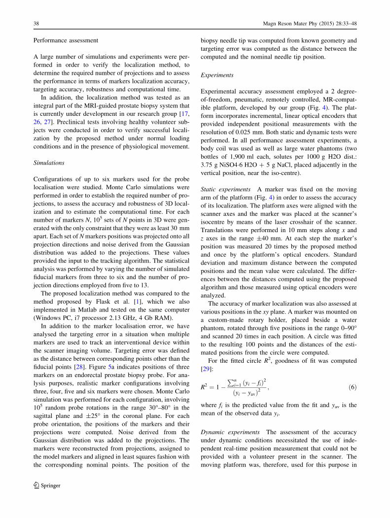
Experiments

Experimental accuracy assessment employed a 2 degree-

of-freedom, pneumatic, remotely controlled, MR-compat-

ible platform, developed by our group (Fig. 4). The plat-

form incorporates incremental, linear optical encoders that

provided independent positional measurements with the

resolution of 0.025 mm. Both static and dynamic tests were

performed. In all performance assessment experiments, a

body coil was used as well as large water phantoms (two

bottles of 1,900 ml each, solutes per 1000 g H2O dist.:

3.75 g NiSO4�6 H2O ? 5 g NaCl, placed adjacently in the

vertical position, near the iso-centre).

Static experiments A marker was fixed on the moving

arm of the platform (Fig. 4) in order to assess the accuracy

of its localization. The platform axes were aligned with the

scanner axes and the marker was placed at the scanner’s

isocentre by means of the laser crosshair of the scanner.

Translations were performed in 10 mm steps along x and

z axes in the range ±40 mm. At each step the marker’s

position was measured 20 times by the proposed method

and once by the platform’s optical encoders. Standard

deviation and maximum distance between the computed

positions and the mean value were calculated. The differ-

ences between the distances computed using the proposed

algorithm and those measured using optical encoders were

analyzed.

The accuracy of marker localization was also assessed at

various positions in the xy plane. A marker was mounted on

a custom-made rotary holder, placed beside a water

phantom, rotated through five positions in the range 0–90�and scanned 20 times in each position. A circle was fitted

to the resulting 100 points and the distances of the esti-

mated positions from the circle were computed.

For the fitted circle R2, goodness of fit was computed

[29]:

R2 ¼ 1�Pn

i¼1 yi � fið Þ2

yi � yavð Þ2; ð6Þ

where fi is the predicted value from the fit and yav is the

mean of the observed data yi.

Dynamic experiments The assessment of the accuracy

under dynamic conditions necessitated the use of inde-

pendent real-time position measurement that could not be

provided with a volunteer present in the scanner. The

moving platform was, therefore, used for this purpose in


123

combination with a large water phantom. Dynamic tests

involved moving a fiducial marker along predefined tra-

jectories in x and z directions at various speeds, while

simultaneously recording the encoder readings and the

estimated fiducial positions.

Application: MRI guided prostate biopsy

The MRI-guided prostate biopsy system employs a remo-

tely operated MRI-compatible manipulator used to position

a detachable endorectal probe that serves as the biopsy

needle guide. Figure 5a shows the set-up in the MR scan-

ner. For the purposes of preclinical testing, we have also

constructed an MRI-visible pelvic model made from sili-

con rubber, which realistically represents the male pelvic

anatomy, both internally and externally, of a person

weighing approximately 70 kg. The overall dimensions of

the model were 50, 50, 20 cm. The model houses anus,

rectum and an empty cavity for placement of a gelatine

assembly which did possess the density and elasticity

properties that mimic the resistance of normal prostate

tissue and have a number of simulated lesions in it. The

model provides realistic displacements of the lesion that

are caused by the probe movement. In addition, the model

accommodates the two large water phantoms described

previously, which provided the loading. This setup was

primarily used to assess the suitability of the manipulator

for use in a limited space and to assess the clinician’s

perception of the situation in a scanner.

The procedure starts by positioning the pelvic phantom

onto the scanner bed and by inserting the probe. The

manipulator is then fixed in place on the scanner bed and

the probe is attached to it. A preoperative set of images is

acquired and the scene is constructed using the transversal

and interpolated coronal cross section through the lesion.

The clinician identifies the lesion to be targeted, interac-

tively selects the target point and starts the targeting.

During the targeting, the scanner streams 1D projections to

the navigation workstation, which computes the probe

position. The 3D synthetic model of the probe is inserted

into the scene in real time and the scene is visualized on the

screen in the scanner room (Fig. 5b). To improve the cli-

nician’s comprehension of the current situation in the

scanner, the oblique cross section, passing through the

markers, is interpolated through the scanned volume every

time new marker positions are obtained. Note that the

scanned volume, the scene and the probe positions are all

computed in the scanner’s coordinate system. To make

targeting easier, the needle is visualized in a position where

it would be if fired. Based on the current position of the

needle in relation to the selected target position, the clini-

cian remotely controls the manipulator and moves the

probe towards a correct firing position.

Before releasing the needle, a verification scan is per-

formed in the same way as the preoperative one. The

position of the targeted lesion is assessed and, if significant

movement is detected, then the whole procedure is repe-

ated until satisfactory targeting is achieved. At that point an

automatic biopsy gun incorporating an extended, MRI

compatible, biopsy needle (InVivo, Germany) is introduced

into the device using an elongated handle. The needle is

fired and the sample is acquired.

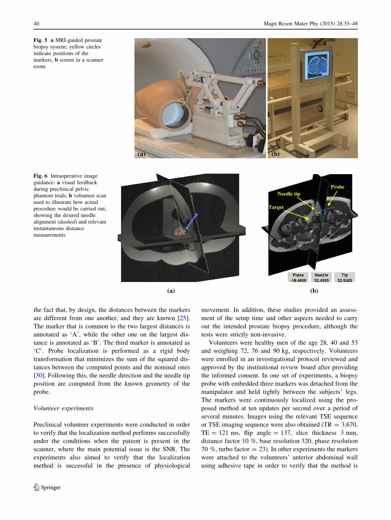
Figure 6a shows the display during the preclinical

phantom trials, while Fig. 6b overlays a 3D model of the

probe onto the volunteer’s scan to show how this may look

in a real situation.

Probe localization during the procedure is performed

using markers built into the probe, Fig. 5a. Importantly, the

manipulator mechanism was designed such that the axes of

the markers are always kept perpendicular to the main

field. In order to compute position and orientation of the

needle, it is necessary to assign the points computed by the

localization method to the corresponding ones on the

nominal model of the probe. The assignment is based on

Fig. 4 MRI-compatible pneumatic moving platform controlled remotely from control room


123

the fact that, by design, the distances between the markers

are different from one another, and they are known [25].

The marker that is common to the two largest distances is

annotated as ‘A’, while the other one on the largest dis-

tance is annotated as ‘B’. The third marker is annotated as

‘C’. Probe localization is performed as a rigid body

transformation that minimizes the sum of the squared dis-

tances between the computed points and the nominal ones

[30]. Following this, the needle direction and the needle tip

position are computed from the known geometry of the

probe.

Volunteer experiments

Preclinical volunteer experiments were conducted in order

to verify that the localization method performs successfully

under the conditions when the patient is present in the

scanner, where the main potential issue is the SNR. The

experiments also aimed to verify that the localization

method is successful in the presence of physiological

movement. In addition, these studies provided an assess-

ment of the setup time and other aspects needed to carry

out the intended prostate biopsy procedure, although the

tests were strictly non-invasive.

Volunteers were healthy men of the age 28, 40 and 53

and weighing 72, 76 and 90 kg, respectively. Volunteers

were enrolled in an investigational protocol reviewed and

approved by the institutional review board after providing

the informed consent. In one set of experiments, a biopsy

probe with embedded three markers was detached from the

manipulator and held tightly between the subjects’ legs.

The markers were continuously localized using the pro-

posed method at ten updates per second over a period of

several minutes. Images using the relevant TSE sequence

or TSE imaging sequence were also obtained (TR = 3,670,

TE = 121 ms, flip angle = 137, slice thickness 3 mm,

distance factor 10 %, base resolution 320, phase resolution

70 %, turbo factor = 23). In other experiments the markers

were attached to the volunteers’ anterior abdominal wall

using adhesive tape in order to verify that the method is

Fig. 5 a MRI-guided prostate

biopsy system; yellow circles

indicate positions of the

markers, b screen in a scanner

room

(b)(a)

Needle tip

Target

Probe

Fig. 6 Intraoperative image

guidance: a visual feedback

during preclinical pelvic

phantom trials; b volunteer scan

used to illustrate how actual

procedure would be carried out,

showing the desired needle

alignment (dashed) and relevant

instantaneous distance

measurements


123

successful in the presence of respiratory movement. Con-

tinuous localization was performed at ten updates per

second over a period of several minutes.

Results

Microcoil characteristics and safety

The Q-factor of the microcoil was found to be around 130

without loading, while when loaded by placing it on top of

a water phantom the Q-factor was found to be around 120.

No measurable temperature change was observed during

the experiments with tracking sequence. For the imaging

sequence a temperature rise of about 0.2 �C was recorded.

Signal analysis

Signal amplitude under repeated excitations

Figure 7 shows simulated and experimentally received

signals, generated by the marker when acquiring a set of 13

projections at different applied flip angles aapp. Simulations

and experiments show that for higher flip angles aapp, the

amplitude of the acquired MR signal is initially larger;

however, for the subsequent acquisitions, the amplitude

drops faster than for smaller flip angles and reaches values

comparable with the measured background signal. The flip

angles aapp for which the signal showed higher minimum

amplitude of signal over the whole set were 0.2� and 0.3�,

the effective flip angle was Q� aapp.

The experimental signal shows an oscillating trend

(Fig. 7b). This was found to be highly repeatable and

dependent on the direction of projection, therefore, it was

attributed to an asymmetry of the markers.

Marker orientation to the main magnetic field

Measured results in Fig. 8 show that for angles up to

50� peaks were always correctly detected for all the

projections. At 60� the amplitude of the peak was com-

parable with the amplitude of the background signal and

the peak was correctly detected in about 60 % of the cases.

Peak detection and sub-pixel localization

Using the position of the pixel with the highest intensity for

peak localization, would lead to a maximum error of 0.5

pixel, or 0.6 mm in this work. By using Gaussian inter-

polation, the maximum peak localization error was reduced

to 0.283 mm (Table 4). The Chi square goodness-of-fit test

showed that the deviation of the peak positions

over repeated acquisition is normally distributed (Fig. 9).

The standard deviation rpeak varied between 0.03 and

0.075 mm. In the experiments with a volunteer in the

scanner the standard deviation reached 0.08 mm.

Peak merging

A situation involving two close peaks is illustrated in

Fig. 10, where the same projection was acquired twice

while the markers were static. In Fig. 10a two high inten-

sity peaks are evident while in Fig. 10b these peaks have

merged into one. It was found that peak merging may

0

0.2

0.4

0.6

0.8

1

1 2 3 4 5 6 7 8 9 10 11 12 13Si

gnal

(a.

u.)

Projection

α=0.1

α=0.2

α=0.3

α=0.4

α=0.5

0

0.2

0.4

0.6

0.8

1

1 2 3 4 5 6 7 8 9 10 11 12 13

Sign

al (

a.u.

)

Projection

α=0.1α=0.2α=0.3α=0.4α=0.5background signal

(b)(a)Fig. 7 Signal variation under

multiple excitations.

a Simulated and

b experimentally acquired

signal for different flip angles

0.000

0.005

0.010

0.015

0.020

0 10 20 30 40 50 60

Sign

al (

a.u.

)

Angle (Degrees)

backgroundsignalpeak amplitude

Fig. 8 The amplitude of a peak decreases for increasing angles to the

main magnetic field


123

happen when peaks are within two pixels from one another

and that the position of the identified peak is not affected

by merging. This phenomenon, however, does not affect

the accuracy in determining the candidate points, and,

therefore, the accuracy of localization, because projections

with less than N peaks are not used in their computation.

The only consequence is that in situations with less than

N peaks along some direction the tolerance needs to be

enlarged to the size of two pixels.

It was also noted that a single marker may cause the

occurrence of two distinct peaks in a single projection. In

all such cases the distance between these two peaks was

exactly one pixel. This can potentially cause serious

problems as a fictitious peak may be higher than some real

peak and, therefore, lead to entirely inaccurate conclusions.

However, this was solved by a simple remedy: if two peaks

are exactly one pixel apart, then the smaller of the two is

neglected. In this way the problem becomes the same as the

one explained above and, as such, it does not affect the

accuracy.

One more effect has been identified that needs attention.

If the density of the material within the coil is non-uniform,

or, if the shape of the material within a coil is not spherical,

the maximum signal intensity may not appear at the centre

of the coil, depending on the orientation of the coil. This

may affect the accuracy of localization—so every effort

has been made to make the shape symmetric and the

homogeneity of the material in the coil uniform, as much as

possible.

Performance assessment

Simulation studies

Robustness and Accuracy The robustness of the proposed

method was expressed in terms of a percentage of suc-

cessful localizations of N markers in a set of experiments.

Table 1 summarizes the results of 106 simulations of

N markers, with N = 3, 4, 5, 6. The number of 1D pro-

jections was increased from five up to 13. These results

show that robustness is improved with an increased number

of projections and that more projections are needed with an

increased number of markers. In all cases simulated vari-

ation in peak localization was rpeak = 0.08 mm.

However, the results in Table 1 should be considered in

relation to the accuracy of results in Fig. 11, showing the

variation of the maximum error as a function of the number

of projections.

Two aspects can be observed. Firstly, although the

algorithm robustness may be already high, the maximum

error may be significantly reduced by increasing the

0

20

40

60

80

100

120

-0.15 -0.1 -0.05 0 0.05 0.1 0.15

Fre

quen

cy

Bin centre (mm)

Observed

Expected

Fig. 9 A number of events from the known distribution expected in

each bin and a number of events observed in each bin

Fig. 10 Identification of close peaks. a Two distinct peaks detected, b single peak detected


123

number of projections, and this is particularly evident for

N [ 3 markers. Secondly, in all cases the results appear to

converge at n ¼ 13, leading to the conclusion that using 13

projections is an optimal choice when up to six markers are

used.

The influence of background noise on the accuracy of

peak detection in 1D projections was explored through

simulations. It was found that the background noise does

influence the accuracy of the sub-pixel peak localization, as

illustrated in Fig. 12.

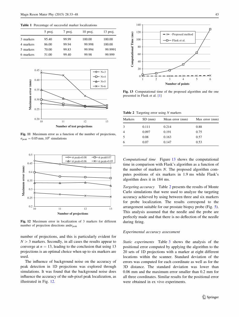
Computational time Figure 13 shows the computational

time in comparison with Flask’s algorithm as a function of

the number of markers N. The proposed algorithm com-

putes positions of six markers in 1.9 ms while Flask’s

algorithm does it in 184 ms.

Targeting accuracy Table 2 presents the results of Monte

Carlo simulations that were used to analyze the targeting

accuracy achieved by using between three and six markers

for probe localization. The results correspond to the

arrangement suitable for our prostate biopsy probe (Fig. 5).

This analysis assumed that the needle and the probe are

perfectly made and that there is no deflection of the needle

during firing.

Experimental accuracy assessment

Static experiments Table 3 shows the analysis of the

positional error computed by applying the algorithm to the

20 sets of 1D projections with a marker at eight different

locations within the scanner. Standard deviation of the

errors was computed for each coordinate as well as for the

3D distance. The standard deviation was lower than

0.06 mm and the maximum error smaller than 0.2 mm for

all three coordinates. Similar results for the positional error

were obtained in ex vivo experiments.

Table 1 Percentage of successful marker localizations

5 proj. 7 proj. 10 proj. 13 proj.

3 markers 95.40 99.99 100.00 100.00

4 markers 86.00 99.94 99.998 100.00

5 markers 70.00 99.83 99.994 99.9991

6 markers 51.00 99.40 99.98 99.999

0.20

0.25

0.30

0.35

0.40

0.45

10 11 12 13

Max

imum

err

or (

mm

)

Number of test projections

N=3

N=4

N=5

N=6

Fig. 11 Maximum error as a function of the number of projections,

rpeak ¼ 0:05 mm; 106 simulations

0.2

0.25

0.3

0.35

0.4

0.45

0.5

10 11 12 13

Max

imum

err

or (

mm

)

Number of projections

σ peak=0.08 σ peak0.07σ peak=0.06 σ peak=0.05

Fig. 12 Maximum error in localization of 3 markers for different

number of projection directions andrpeak

0

20

40

60

80

100

120

140

1 2 3 4 5 6

Com

puta

tion

al T

ime

(ms)

Number of points

Proposed method

Flask et al.

Fig. 13 Computational time of the proposed algorithm and the one

presented in Flask et al. [1]

Table 2 Targeting error using N markers

Markers SD (mm) Mean error (mm) Max error (mm)

3 0.111 0.214 0.88

4 0.097 0.191 0.75

5 0.08 0.163 0.57

6 0.07 0.147 0.53


123

Figure 14 shows a representative subset of the distance

errors computed as the difference between distances cal-

culated using marker tracking and those obtained by optical

encoders. Error contribution due to an imperfect alignment

of the platform with the scanner axes was assumed to be

negligible.

The corresponding statistics for independent translations

in the x and z directions are presented in Table 4. The

average translational error was 0.056 mm while the max-

imum error was smaller than 0.3 mm. These experiments

indicate that sub-millimetre accuracy in tracking can be

achieved using the proposed method. It can also be

observed that the standard deviation of the distance error is

larger than that of the position error shown in Table 3. This

is in agreement with the theory which states that, for

independent random variables x and y, the variance of their

sum or of their difference is the sum of individual vari-

ances, (i.e.,r2XþYð Þ ¼ r2

X�Yð Þ ¼ r2X þ r2

Y ).

Figure 15 illustrates the results of the localization where a

fiducial marker was positioned in five different positions (20

times in each) on a circle in the xy plane. High accuracy of

localization is proved by computing the goodness of fit of the

100 measured points to the ideal circle R2 = 0.9979.

Dynamic experiments The results of dynamic tests,

involving controlled movement of the platform carrying

the marker at different speeds are shown in Fig. 16. While

the platform was moving, sets of 13 1D projections were

repeatedly acquired at regular intervals of 500 ms. The

instantaneous position was measured by the encoders after

the acquisition of the 6th projection, in order to reduce the

time delay between the locations obtained in the two ways.

Table 5 reports the mean and maximum error at the

different speeds of the platform. The reported speed is the

maximum speed achieved using the s-shaped velocity

profile and was controlled by the platform controller. At

40 mm/s the error is lower than 1 mm; at higher speeds, the

error increases up to a few mm.

Application: MRI guided prostate biopsy

The MRI guided biopsy procedure was carried out in five

trials, involving the integrated system and the use of the

pelvic model and the prostate phantoms described previ-

ously. A trial was considered to be successful if the target

sample was acquired, which was evident from its colour,

and this was achieved in all trials. Figure 17a presents a

sagittal MR image scanned after firing. Figure 17b presents

the prostate gland phantom incorporating a 4 mm diameter

spherical lesion with the needle track clearly visible.

During targeting, the displayed images of the needle

appeared somewhat jittery due to the noise, so a moving

average filter that averages five samples was implemented.

The stability of the images was improved noticeably, but at

the expense of introducing an error due to the delay in the

Table 3 Positional error

x Y z 3D

Standard deviation (mm) 0.024 0.040 0.058 0.037

Maximum error (mm) 0.105 0.090 0.148 0.208

-0.25

-0.2

-0.15

-0.1

-0.05

0

0.05

0.1

0.15

0.2

0.25

1 16 31 46 61 76 91 106 121 136

Dis

tanc

e er

ror

(mm

)

Measurement number

Fig. 14 Distance error for a subset of 140 measurements along x.

Each point is computed as the difference between distances calculated

with marker tracking and those measured with optical encoders

Table 4 Distance error statistic: mean error, standard deviation and

maximum error

x translation z translation

Mean error (mm) 0.049 -0.063

Standard deviation (mm) 0.098 0.168

Maximum error (mm) 0.216 0.283

Fig. 15 Estimated marker positions and fitted circle. Each position is

measured 20 times


123

computed positions. Conveniently, this error diminishes as

the movement becomes slower in the final phase of the

targeting.

Volunteer experiments

In all experiments involving volunteers the localization

method was found to perform successfully, without fail-

ures, i.e., correct peaks were always identified under pro-

longed operation lasting several minutes. Experiments

involving the biopsy probe taped and held tightly between

the subject’s legs showed that the SNR of the marker signal

was sufficiently high under coil loading and noise condi-

tions similar to that during the intervention. When the

markers were taped to the subject’s anterior abdominal

wall, where maximum motion artefacts might be expected

due to the respiratory motion, the results did not indicate

any signal smearing and the localization performed equally

successfully over periods of several minutes.

Discussion

The localization method described here has been shown to

be both accurate and fast, while being able to track

N markers simultaneously.

Accuracy and robustness

Using a set of 13 pre-defined 1D projections was shown to

be optimal in terms of minimizing the localization error

and maximizing the robustness, while the penalty in terms

of computational time was minimal. The number of pro-

jections can be traded against robustness and accuracy for

0

20

40

60

80

100

500 1500 2500 3500 4500 5500

Pos

itio

n (m

m)

Time (ms)

40mm/s

EncodersMarker

0

20

40

60

80

100

500 1500 2500 3500

Pos

itio

n (m

m)

Time (ms)

60mm/s

(a)

(b)

0

20

40

60

80

100

500 1000 1500 2000 2500

Pos

itio

n (m

m)

Time (ms)

120mm/s(c)

Fig. 16 Dynamic tracking at different speeds. Estimated marker

positions and measured by encoders

Table 5 Distance error for increasing speed

40 mm/s 60 mm/s 120 mm/s

Mean error (mm) 0.39 1.17 3.07

Max error (mm) 0.72 3.65 7.81

Fig. 17 Targeting results: a sagittal MR image after firing; b photo of the actual target used in the experiment, with the needle track visible


123

optimized results in a specific situation. Furthermore, by

using the Gaussian interpolation the accuracy of the posi-

tion of the peak estimation was significantly improved

compared to using the Maximum Pixel Intensity method.

The algorithm is heuristic and two failure modes were

identified. First, the algorithm fails if any two markers are

positioned too close to each other in relation to the toler-

ance e. In practice this problem is unlikely and it may be

readily solved by adequately placing the markers on the

instrument. The second failure mode is related to a situa-

tion where symmetries exhibited by the arrangement of the

markers and the chosen directions of the projections gen-

erate too many coincident peaks, such that the remaining

projections cannot remove all of the fictitious points. This

may be solved by choosing a more suitable marker

arrangement for the given application or by changing the

projection directions in a way that would break the

symmetries.

Determination of the tolerance

Optimizing the value of the tolerance e is an important but

complex problem to address. Too small a value for e will

remove too many candidate points whereas too large e will

keep some fictitious points in. Our experiments and simu-

lations indicated that the main factors to be considered

when determining the tolerance value are the stochastic

nature of the peak position and the identification of peaks

that are very close to each other.

By setting the tolerance to ten standard deviations, the

stochastic nature was resolved. However, the situation is

different when the two peaks are close to each other. It was

found that peak merging may occur when peaks are within

two pixels from one another and that the position of the

identified peak is not affected by merging. In order to

accommodate peak merging, the tolerance was automati-

cally enlarged to two pixels size in situations where fewer

than N peaks are detected. In this way, merged peaks were

represented by the identified one. This solution did not affect

the accuracy nor robustness of our localization method, since

the candidate points are computed by making use only of the

projections that do have N distinct peaks.

It is well known [31] that positional errors may result

from resonance offset errors, such as those when the

markers are in a region of an inhomogeneous field near the

edges of the imaging volume, or in regions with magnetic

distortions caused by differences in magnetic susceptibility.

This positional error may affect the robustness of our

method, because in the test projections it may change the

distance between a projected candidate point and its cor-

responding peak. If this causes the tolerance to be exceeded,

then some of the correct points may be wrongly removed.

One way to remedy this problem is to increase the tolerance.

Application in MRI-guided interventional procedures

The proposed method may be applied to localize either

semi-active or active markers, when only one receiver

channel is used. However, we have focused on the use of

semi-active markers, as it simplifies the instrument design,

manufacturing and testing, and avoids cabling issues and

the associated safety hazards [32]. We have experienced no

significant heating at the relatively low RF exposure levels

used in our experiments. The dimensions and the flexibility

of use of the semi-active markers make them particularly

suitable for MRI-guided interventions involving small

devices.

It was observed that, when a human subject is present in

the scanner, the peak amplitude of the marker signal may

decrease, but it was still sufficiently high for the peak

detection method to function correctly and consistently. In

practice, obtaining a sufficiently strong signal from the

markers can always be expected to be a concern, so the

interventional system should be designed such that this is not

compromised. Marker orientation to the main field is a key

aspect and it is preferable to adopt a manipulator configu-

ration that ensures that markers are always kept perpendic-

ular to B0, as was the case in the prostate biopsy system.

The dynamic tracking test proved the reliability of the

method in the presence of motion, with accuracy depending

on the speed. For the anticipated speeds of tool movement

in interventional procedures, the marker positional error

was estimated to be within 1 mm.

In preclinical trials the targeting time for prostate biopsy

was found to be of the order of 5 min. The proposed

prostate biopsy MR-guided method was considered by the

clinical staff to offer significant advantages in terms of

being able to target previously identified lesions, avoiding

the need for extensive random sampling and increasing the

accuracy of the biopsies.

Targeting errors such as those due to mechanical deflec-

tion of the needle during firing have not been assessed and are

potentially significant. Under these conditions, pre-clinical

trials were conducted to investigate the ability to success-

fully sample small targets, of the size specified by the cli-

nician as being clinically relevant. Although these trials were

successful, a detailed accuracy of the interventional system

needs to be carried out as part of future work, in order to fully

assess the errors and influence of factors such as needle firing

speed and tissue properties.

In the proposed prostate biopsy procedure, the anatom-

ical MR images are only acquired near the start of the

intervention, just before the targeting begins, and imme-

diately before a possible needle release. In the latter case

the images are used for the verification of the targeting

before the needle is released. Both stages involve obtaining

multiple images across the volume of interest, in which the


123

clinician recognizes and identifies the target lesion. In this

situation the main benefit of the high update rate of the

probe tracking is an improved control of the probe position.

In other applications it may be required to update specific

MR images simultaneously with tracking, so the faster

localization method will help improve the overall image

acquisition speed.

Preclinical trials have also revealed that the noise in the

system may result in a noticeable jitter in the estimated

position of the probe, which may prove distracting to the

clinician, especially when performing fine adjustments of

the manipulator during targeting. This was easily overcome

by implementing a simple moving average filter, resulting

in a much steadier display. As a consequence of the fast

sampling time (10 Hz), averaging of the last five positions

and the slow movement of the probe in the final phase of a

targeting, the lag introduced by filtering was not noticeable

and it did not impede operator’s actions in any way. The

use of the Kalman filter would be an optimal solution for

this problem and it will be considered in the next stages of

system development.

Conclusion

A method for localization of N markers in 3D based on a

novel algorithm for processing 1D projections was presented

and proved to be considerably faster than previously pro-

posed methods. Computational time for up to six markers

required less than 2 ms. High accuracy was achieved by

using optimal reference projections to compute candidate

points and by applying Gaussian interpolation in peak

detection. An update rate of 10 Hz was achieved with

localization error lower than 0.3 mm. The reliability of the

method when markers move while performing an interven-

tion was demonstrated and resulted in maximum error

0.7 mm for a speed anticipated by interventional procedures.

Experimental targeting error was estimated to be about

1 mm and, we predict a reduction of up to two times by

employing up to six markers. An important aspect of the

manipulator design is that its remote-centre mechanism

maintains the orientation of the markers perpendicular to the

main field in all positions, maximizing the peak amplitudes

during tracking. Accurate marker localization leads to

accurate accurate and consistent targeting in MR guided

interventions, while the speed of the method enables high

frame-rate display that is comfortable for the clinician and

enhances the overall performance.

Acknowledgments This work has been conducted under funding

from the Translation Award of The Wellcome Trust, for which we are

grateful. Special thanks to Pedro Ferreira (Imperial College London,

Medicine, London, UK) for the technical support.

Open Access This article is distributed under the terms of the

Creative Commons Attribution License which permits any use, dis-

tribution, and reproduction in any medium, provided the original

author(s) and the source are credited.

References

1. Flask C, Elgort D, Wong E, Shankaranarayanan A, Lewin J,

Wendt M, Duerk JL (2001) A method for fast 3D tracking using

tuned fiducial markers and a limited projection reconstruction

FISP (LPR-FISP) sequence. J Magn Reson Imaging 14(5):

617–627

2. Reither K, Wacker F, Ritz JP, Isbert C, Germer CT, Roggan A,

Wendt M, Wolf KJ (2000) Laser-induced thermotherapy (LITT)

for liver metastasis in an open 0.2T MRI. Abteilung fur Radiol-

ogie und. Nuklearmedizin 172(2):175–178

3. Moore P (2005) MRI-guided congenital cardiac catheterization

and intervention: the future? Catheterization and cardiovascular

interventions. J Soc Card Angiogr Interv 66(1):1–8

4. Mortele KJ, Tuncali K, Cantisani V, Shankar S, vanSonnenberg

E, Tempany C, Silverman SG (2003) MRI-guided abdominal

intervention. Abdom Imaging 28(6):756–774

5. Damianou C, Ioannides K, Mylonas N, Hadjisavas V, Couppis A,

Iosif D (2009) Liver ablation using a high intensity focused

ultrasound system and MRI guidance. In: Proceedings of the 9th

international conference on information technology and applica-

tions in biomedicine, Larnaca, Cyprus, p 490–493

6. Breen MS, Butts K, Chen L, Saidel GM, Wilson DL (2004) MRI-

guided laser thermal ablation: Model to predict cell death from

MR thermometry images for real-time therapy monitoring. In:

Proceedings of the 26th international conference of the IEEE,

p 1028–1031

7. Larson BT, Tsekos NV, Erdman AG (2003) A robotic device for

minimally invasive breast interventions with real-time MRI

guidance. In: Proceedings of the 3rd scientific meeting, IEEE

symposium on bioinformatics and bioengineering, p 190–197

8. Krieger A, Susil RC, Menard C, Coleman JA, Fichtinger G, At-

alar E, Whitcomb LL (2005) Design of a novel MRI compatible

manipulator for image guided prostate interventions. IEEE Trans

Biomed Eng 52(2):306–313

9. Tadayyon H, Lasso A, Kaushal A, Guion P, Fichtinger G (2011)

Target motion tracking in MRI-guided transrectal robotic prostate

biopsy. IEEE Trans Biomed Eng 58(11):3135–3142

10. Xu H, Lasso A, Vikal S, Guion P, Krieger A, Kaushal A,

Whitcomb LL, Fichtinger G (2010) MRI-guided robotic prostate

biopsy: a clinical accuracy validation. Med Image Comput

Comput Assist Interv 13(Pt 3):383–391

11. Dumoulin CL, Souza SP, Darrow RD (1993) Real-Time position

monitoring of invasive devices using magnetic-resonance. Magn

Reson Med 29(3):411–415

12. Krieger A, Metzger G, Fichtinger G, Atalar E, Whitcomb LL

(2006) A hybrid method for 6-DOF tracking of MRI-compatible

robotic interventional devices. In: Proceedings of the IEEE

international conference robotics and automation, Orlando,

Florida, pp 3844–3849

13. de Oliveira A, Rauschenberg J, Beyersdorff D, Semmler W, Bock

M (2008) Automatic passive tracking of an endorectal prostate

biopsy device using phase-only cross-correlation. Magn Reson

Med 59(5):1043–1050

14. DiMaio S, Samset E, Fischer G, Lordachita I, Fichtinger G,

Jolesz F, Tempany CM (2007) Dynamic MRI scan plane control

for passive tracking of instruments and devices. Med Image

Comput Comput Assisted Interv MICCAI 10(2):50–58


123

15. Burl M, Coutts GA, Young IR (1996) Tuned fiducial markers to

identify body locations with minimal perturbation of tissue

magnetization. Magn Reson Med 36(3):491–493

16. Brujic D, Galassi F, Rea M, Ristic M (2012) A novel algorithm

for fast 3D localization of N fiducial markers from 1D projec-

tions. In: Proceedings of 20th scientific meeting, international

society for magnetic resonance in medicine, Melbourne, p 2946

17. Brujic D, Galassi F, Rea M, DeSouza N, Rristic M (2013) Novel

surgical assistance system for MRI-guided prostate biopsy. In:

Proceedings of the Interventional oncology sans frontieres con-

gress, Cernobbio, Italy, p 90

18. Glassner S (1990) Graphic gems. Academic Press, New York

19. Toriwaki J, Yoshida H (2009) Fundamentals of three-dimensional

digital image processing. Springer, London, New York

20. Rea M, McRobbie D, Elhawary H, Tse Z, Lamperth M, Young I

(2009) Sub-pixel localization of passive micro-coil fiducial

markers in interventional MRI. Magn Reson Mater Phy

22(2):71–76

21. Garnov N, Thormer G, Trampel R, Grunder W, Kahn T, Moche

M, Busse H (2011) Suitability of miniature inductively coupled

RF coils as MR-visible markers for clinical purposes. Med Phys

38(11):6327–6335

22. Bernstein MA, King KF, Zhou ZJ (2004) Handbook of MRI pulse

sequences. Academic Press, Amsterdam, Boston

23. Hargreaves BA, Vasanawala SS, Pauly JM, Nishimura DG

(2001) Characterization and reduction of the transient response in

steady-state MR imaging. Magn Reson Med 46(1):149–158

24. R. B. Fisher D K Naidu (1996) A comparison of Algorithms for

subpixel peak detection. In: Sanz J (ed) Image technology,

advances in image process, multim and machine vision. Springer,

New York, pp 385–404

25. Zhang Q, Wendt M, Aschoff AJ, Lewin JS, Duerk JL (2001) A

multielement RF coil for MRI guidance of interventional devices.

J Magn Reson Imaging 14(1):56–62

26. Lambert N, Ristic M, Desouza N (2012) Design of a novel device

for MRI guided transrectal prostate biopsy. In: Proceeding of the

9th international MRI symposium, Boston, MA, p 58

27. Galassi F, McGinley J, Ristic M, Desouza N, Brujic D (2013)

Design of a receiver array for MRI-guided transrectal prostate

biopsy. In: Proceedings of 21st scientific meeting, international

society for magnetic resonance in medicine, Salt lake City,

p 2730

28. Fitzpatrick M, West B (2001) The distribution of target regis-

tration error in rigid-body point-based registration. IEEE Trans

Med Imaging 20(9):917–927

29. Utts JM, Heckard RF (2006) Statistical ideas and methods.

Thomson-Brooks/Cole, Belmont

30. Arun KS, Huang TS, Blostein SD (1987) Least-squares fitting of

two 3-d point sets. IEEE Trans Pattern Anal Mach Intell

9(5):698–700

31. Wang D, Strugnell W, Cowin G, Doddrell DM, Slaughter R (2004)

Geometric distortion in clinical MRI systems part I: evaluation

using 3D phantom. Magn Reson Imaging 22:1211–1221

32. Nitz WR, Oppelt A, Renz W, Manke C, Lenhart M, Link J (2001)

On the heating of linear conductive structures as guide wires and

catheters in interventional MRI. J Magn Reson Imaging

13(1):105–114


123

Fast and accurate localization of multiple RF … · Fast and accurate localization of multiple RF...

Documents

Transcript of Fast and accurate localization of multiple RF … · Fast and accurate localization of multiple RF...