1

FAST AND ACCURATE CALCULATION OF OWEN’S T-FUNCTION

MIKE PATEFIELD

Department of Applied StatisticsThe University of Reading, UK

and

DAVID TANDY

Millward BrownWarwick, UK

Address for Correspondence: Department of Applied Statistics,The University of Reading, PO Box 240,Earley Gate, Reading RG6 6FN, UK

e-mail: w.m.patefield@reading.ac.uk and david.tandy@uk.millwardbrown.com

Keywords: T-function; Bivariate normal probabilities

DESCRIPTION AND PURPOSE

Given values of h and a, the function T calculates

2 211 2

2 0

exp{ (1 )}( ) (2 ) ( , )

1− − +

= − ∞ < < +∞+∫

a h xT h,a dx h a

xπ (1)

Owen (1956, equation 3.4 and Figure 1) gives an alternative formulation of T(h,a) in terms of

an integral over an area of the standardized bivariate normal distribution with zero

correlation. Cooper (1968b) has provided an algorithm FUNC for calculating T(h,a) using an

approximation due to Nicholson (1943) and a series expansion based on equation (3.9) of

Owen (1956). This algorithm is unsatisfactory for large values of h. Young and Minder

(1974) and Thomas (1986) use 10 point Gaussian quadrature in their functions TFN and

2

TFNX. The accuracy of these is limited by the accuracy of the quadrature points and weights

used.

The function T listed here uses six methods of evaluation, selecting the appropriate method

for the given values of h and a. A relative error of less than 75 times the machine precision is

attained on a machine working up to at least 16 figure accuracy.

The T-function is used to calculate bivariate normal probabilities, (Sowden and Ashford,

1969; Donelly, 1973) which in turn are used to calculate multivariate normal probabilities,

(Schervish, 1984). A wide variety of uses of bivariate normal probabilities including

applications to measurement errors, calibration and quality control are described by Owen

(1959). A further use of the T-function is in evaluating the non-central t-distribution (Cooper,

1968c).

Maximizing likelihood functions which are in turn functions of bivariate normal probabilities

is made considerably easier when such probabilities are evaluated to high accuracy,

especially when this can be done efficiently.

METHOD

The required range of evaluation of T(h,a) is reduced from (− ∞ < h, a < ∞) to (h ≥ 0,

0 ≤ a ≤ 1) by utilising in turn the following results given by Owen (1956)

T(h, −a) = −T(h, a)

T(−h, a) = T(h, a) (2)

T(h, a) = 12 Φ(h) + 1

2 Φ(ah) − Φ(h) Φ(ah) − T(ah, 1/a),

where Φ(.) denotes the cumulative distribution function of the standard normal distribution.

3

The six methods of calculation of T(h, a) over h ≥ 0, 0 ≤ a ≤ 1 are:-

T1: Evaluation of the first term m terms of the series expansion given by Owen (1956,

equation (3.9)) i.e.

( ) 1 1 2 -1

1( ) 2 tan ( ) /(2 -1)− − = +

∑m

jj

j=

T1 h,a,m a d a jπ

where

( ) ( ) ( )1

2 21 12 2

01 1 exp h /

−

=

= − − −

∑j ij

ji

d h i! (3)

T2: Approximating ( ) 121−

+ x by terms up to order 2m in a power series expansion, i.e.

( ) ( )1112 2

11

−+−

=+ ≈ −∑

im

i

x x

and integrating (1) gives

( ) ( ) ( ) ( )+11/ 2 121

21

2 exp 1−

== − −∑

m i-

ii

T2 h,a,m h zπ

where

( ) ( )1/ 2 2( 1) 2 2120

2 exp ; 1− −= − ≥∫a

iiz x h x dx i π (4)

and hence

{ }11 2( ) /= −z ah hΦ

( ){ }1/ 2 2 1 2 2 211 2(2 1) (2 exp / ; 1− −

+ = − − ) − ≥ii iz i z a a h h iπ .

T3: Approximating ( ) 121+−

x by the polynomial of degree 2m in x which minimizes the

maximum absolute error over [−1, 1], Hornecker (1958) i.e.

( ) 112 2( 1)2

11

+− −

=+ ≈ ∑

mi

ii

x C x .

The coefficients {C2i} are obtained from the coefficients of Chebyshev polynomials as

detailed by Borth (1973). Note the minor change in notation in that Borth denotes C2i above

by C2(i−1). Integrating (1) gives

4

( ) ( ) 11/ 2 2122

1( , , ) 2 exp

+−

== − ∑

m

i ii

T3 h a m h C zπ (5)

where zi is given by (4).

T4: The expression for zi given by (4) may be re-arranged as

( ) ( )1/ 2 (2 1) 2 2 2 111,2

12 exp ( ) ; 1

∞− − − +−

= −= − ≥∑i k

i i kk i

z h a h ah iπ γ (6)

where

1(2 1)−

== +∏

!

!k

jkj

γ (0 ≤ j ≤ k < ∞).

Using

( ) ( )12 2

01

∞−

=+ = −∑

i

i

x x 2 < 1x

and integrating (1) gives

( ) ( ) ( )1/ 2 2112

0( , ) 2 exp 1

∞−+

== − −∑ i

ii

T h a h zπ 1.<a

Substituting for 1z +i using (6) and re-arranging results in

( ) ( ){ } ( ) ( )1 2 2 2 212

0 =0( , ) 2 exp 1 -

∞ −−

== − + −∑ ∑

ii i j

jii j

T h a a h a a hπ γ

which is approximated to order 2m + 1 in a by

( ) ( ){ } ( )1 2 2 212

0( , , ) 2 exp 1−

== − + −∑

m i

ii

T4 h a m a h a a yπ

where

( )2

0

−

== −∑

i i j

i jij

y hγ i ≥ 0

i.e. ( )20 11; 1 /(2 1);−= = − +i iy y h y i i ≥ 1.

T5: Gauss’ 2m-point quadrature formula for approximating the integral of an arbitrary

function f(x) over [−1, 1] is

1

1( )

−≈∫ f x dx { }

1 =1( ) ( ) ( )

== + −∑ ∑

2m m

i i i i ii i

w f x w f x f x (7)

5

where values of the abcissas, xi, and weights, wi are given, for example by Abramowitz and

Stegun (1965). For f(x) = ( ){ } ( )2 2 212exp 1 / 1− + +h x x

( ) ( ) { }11 1

0 1( , ) 2 ( ) 2 ( / 2) (1 ) / 2− −

−= π = π +∫ ∫

a

T h a f x dx a f a x dx .

Using (7) this is approximated by

( ) { } { }1

12 ( / 2) (1 ) / 2 (1 ) / 2−

= + + − ∑

m

i i ii

a w f a x f a xπ (8)

which is the expression utilised by Young and Minder (1974) and Thomas (1986). However,

as f(x) is an even function a computationally simpler approximation is obtained using

( ) ( )11 1

0 1( , ) 2 ( ) 2 ( / 2) ( )− −

−= π = π∫ ∫

a

T h a f x dx a f ax dx .

Using (7) to approximate this integral results in

( ){ } ( )2 2 2 2 212

1( , , ) ( / 2 )exp 1 1

== − + +∑

m

i i ii

T5 h a m a w h a x a xπ .

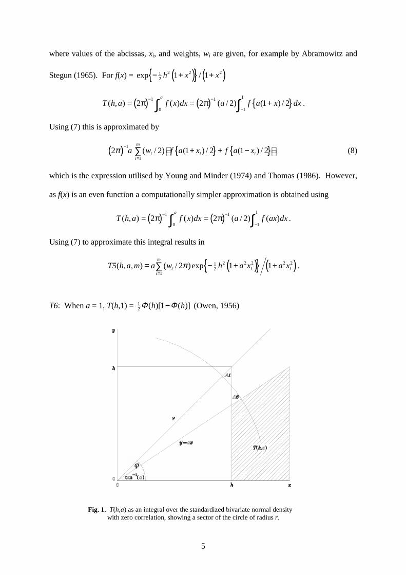
T6: When a = 1, T(h,1) = 12 ( )[1 ( )]−h hΦ Φ (Owen, 1956)

φ

Fig. 1. T(h,a) as an integral over the standardized bivariate normal densitywith zero correlation, showing a sector of the circle of radius r.

6

When a is near one a geometrical argument similar to that of Cadwell (1951) is used. For X,

Y independent standard normal variables, from Owen (1956)

T(h,a) = P(X ≥ h, 0 ≤ Y ≤ aX); 0 ≤ a < 1

Hence

T(h,a) = T(h,1) − P(X ≥ h, aX ≤ Y ≤ X).

Transforming X,Y to independent variables 2 2 1/ 2 1( ) , = tan ( / )−= +R X Y Y Xθ

T(h,a) = T(h,1) − P(R2 ≥ r2 , tan−1(a) ≤ θ ≤ π/4)

+ P(X,Y ε A1) − P(X,Y ε A2)

Figure 1 illustrates the regions A1 and A2 and an arc of the circle of radius r for which A1 and

A2 are of equal area, i.e.

r2 = h2(1 − a)/φ

where φ = π/4 − tan−1(a) = tan−1{(1 − a)/(1 + a)}.

As 2 22~ ,χR θ ~ U(0,2π) and the bivariate normal density of X and Y is smaller throughout A1

than at any point in A2,

( ) ( )1 212( , ) ( ,1) 2 exp−< − −T h a T h rπ φ .

This upper bound on T(h,a) is used as an approximation for a near 1, i.e.

( ) 1 1 2 11 12 2

1 1( , ) ( )[1 ( )] 2 tan exp (1 ) tan1 1

− − − − − = − − − − + a a

T6 h a h h a h+ a a

Φ Φ π .

T7: In addition the following expression for T(h,a) is useful in evaluating T(h,a) accurately.

Substituting equation (6) for zi into (5)

( ) { }min( , ) 11 2 2 1 2( 1)1

2 1,20 1

( ) 2 exp (1 )+∞− − +

−= =

− + ∑ ∑k m

2k+ k ii i k

k i

T7 h,a,m = h a a C hπ γ (9)

i.e.0

( , , ) =∞

=∑ k kk

T7 h a m u v

7

where ( ) { }1 2 2 210 122 exp (1 ) ; , 1−

−= − + = ≥k ku a h a u a u kπ

and 0 21=v C

21 2, 1

k 21

[ ] /(2 1) = 1,...,/(2 1)

− +

−

+ += +

k k

k

h v C k k mv

h v k k > m

This computational procedure for T(h,a) is not incorporated into the code for the function T,

but was used in high precision calculations for validation purposes.

Fig. 2. Method used for computing T(h,a), (h ≥ 0, a ≥0).Key: 1 = (Method 1, Order 2); 2 = (1,3); 3 = (1,4); 4 = (1,5); 5 = (1,7); 6 = (1,10);

7 = (1,12); 8 = (1,18); 9 = (2,10); 10 = (2, 20); 11 = (2,30); 12 = (3,20);13 = (4,4); 14 = (4,7); 15 = (4, 8); 16 = (4, 20); 17 = (5,13); 18 = (6,0).

8

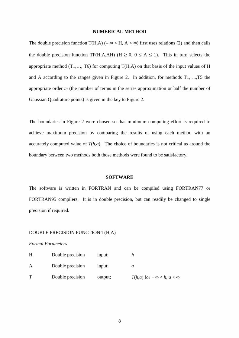
NUMERICAL METHOD

The double precision function T(H,A) (– ∞ < H, A < ∞) first uses relations (2) and then calls

the double precision function TF(H,A,AH) (H ≥ 0, 0 ≤ A ≤ 1). This in turn selects the

appropriate method (T1,…, T6) for computing T(H,A) on that basis of the input values of H

and A according to the ranges given in Figure 2. In addition, for methods T1, ...,T5 the

appropriate order m (the number of terms in the series approximation or half the number of

Gaussian Quadrature points) is given in the key to Figure 2.

The boundaries in Figure 2 were chosen so that minimum computing effort is required to

achieve maximum precision by comparing the results of using each method with an

accurately computed value of T(h,a). The choice of boundaries is not critical as around the

boundary between two methods both those methods were found to be satisfactory.

SOFTWARE

The software is written in FORTRAN and can be compiled using FORTRAN77 or

FORTRAN95 compilers. It is in double precision, but can readily be changed to single

precision if required.

DOUBLE PRECISION FUNCTION T(H,A)

Formal Parameters

H Double precision input; h

A Double precision input; a

T Double precision output; T(h,a) for − ∞ < h, a < ∞

9

DOUBLE PRECISION FUNCTION TF(H,A,AH)

Formal Parameters

H Double precision input; h (h ≥ 0)

A Double precision input; a (0 ≤ a ≤ 1)

AH Double precision input; a × h

TF Double precision output; T(h,a) for h ≥ 0, 0 ≤ a ≤ 1

Failure indications: None. Function TF does not check that h and a are in the required

ranges or that AH is equal to a × h as these are unnecessary when called from T.

Auxiliary algorithms: Functions T and TF require algorithms for calculating the standard

normal integrals

ZNORM1(x) = P(0 ≤ Z ≤ x); ZNORM2(x) = P(x ≤ Z < ∞)

where Z is standard normal. These have been given in the statement functions

ZNORM1(x) = 1 12 2erf ( / 2); ZNORM2( ) = erfc( / 2)√ √x x x

using N.A.G. (1997) library routines S15AEF and S15ADF respectively and can readily be

replaced by the built-in functions ERF and ERFC if available or by routines, for example

function ALNORM of Algorithm AS66, Hill (1973), for calculating the normal integral.

However, using

ZNORM1(x) = ALNORM(x,.FALSE.) − 0.5; ZNORM2(x) = ALNORM(x,.TRUE.)

will at best achieve 12 figure accuracy and also incur additional errors in ZNORM1(x) for x

small. Other methods of calculating the normal integral are given by Cooper (1968a), Adams

(1969), Hill and Joyce (1967) and Kerridge and Cook (1976). Double precision versions of

the functions ERF and ERFC are in the DCDFLIB library of routines for Cumulative

10

Distribution Functions which contains source in FORTRAN77 and documentation. It is

downloadable from the website http://odin.mdacc.tmc.edu/anonftp/page_2.html

The built-in routines DABS (used by T) and DEXP, DATAN and DFLOAT (used by TF) are

declared in statement functions prior to the executable commands in order that they may

readily be changed from double precision.

Constants: All double precision constants are declared in DATA statements so that they may

easily be changed to single precision. These include

RTWOPI = ( ) 12 −π ; RRTPI = ( ) 1/ 22 −π ; RROOT2 = 2−1/2;

the array C2 of 21 coefficients required for T3(h,a,20) and the length 13 arrays PTS and WTS

given by PTS(i) = 2ix , WTS(i) = / 2iw π required for T5(h,a,13). All double precision

constants are given to 20 figures accuracy.

RESTRICTIONS

The input values of h and a should be such that overflow does not occur when calculating h2,

ah, or a2. A value of zero (underflow) is returned for values of h and a for which |T(h,a)| is

less than the smallest double precision number that can be stored.

PRECISION

The software has been developed and tested on a VAX 750 in double precision using 64 bit

real arithmetic (the N.A.G Library being implemented in double precision). Single precision

should be used on machines that achieve this accuracy without resorting to double precision.

If S15AEF and S15ADF are required the N.A.G Library will generally be implemented in

single precision on such machines.

11

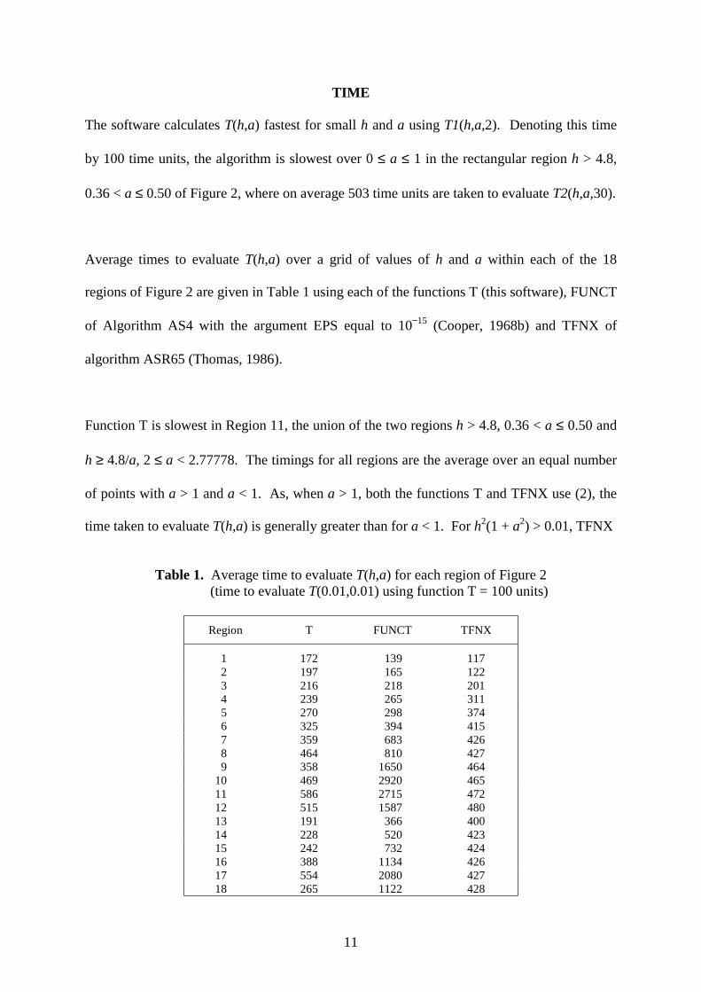
TIME

The software calculates T(h,a) fastest for small h and a using T1(h,a,2). Denoting this time

by 100 time units, the algorithm is slowest over 0 ≤ a ≤ 1 in the rectangular region h > 4.8,

0.36 < a ≤ 0.50 of Figure 2, where on average 503 time units are taken to evaluate T2(h,a,30).

Average times to evaluate T(h,a) over a grid of values of h and a within each of the 18

regions of Figure 2 are given in Table 1 using each of the functions T (this software), FUNCT

of Algorithm AS4 with the argument EPS equal to 10−15 (Cooper, 1968b) and TFNX of

algorithm ASR65 (Thomas, 1986).

Function T is slowest in Region 11, the union of the two regions h > 4.8, 0.36 < a ≤ 0.50 and

h ≥ 4.8/a, 2 ≤ a < 2.77778. The timings for all regions are the average over an equal number

of points with a > 1 and a < 1. As, when a > 1, both the functions T and TFNX use (2), the

time taken to evaluate T(h,a) is generally greater than for a < 1. For h2(1 + a2) > 0.01, TFNX

Table 1. Average time to evaluate T(h,a) for each region of Figure 2(time to evaluate T(0.01,0.01) using function T = 100 units)

Region T FUNCT TFNX

1 172 139 1172 197 165 1223 216 218 2014 239 265 3115 270 298 3746 325 394 4157 359 683 4268 464 810 4279 358 1650 464

10 469 2920 46511 586 2715 47212 515 1587 48013 191 366 40014 228 520 42315 242 732 42416 388 1134 42617 554 2080 42718 265 1122 428

12

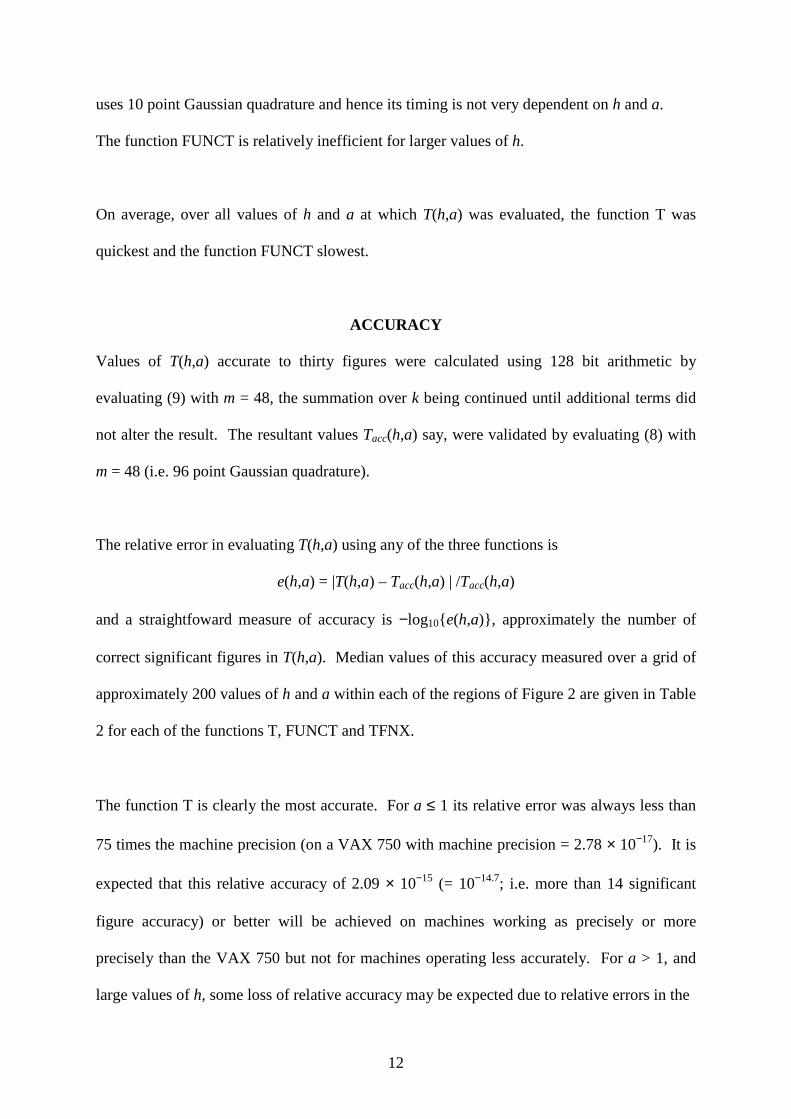
uses 10 point Gaussian quadrature and hence its timing is not very dependent on h and a.

The function FUNCT is relatively inefficient for larger values of h.

On average, over all values of h and a at which T(h,a) was evaluated, the function T was

quickest and the function FUNCT slowest.

ACCURACY

Values of T(h,a) accurate to thirty figures were calculated using 128 bit arithmetic by

evaluating (9) with m = 48, the summation over k being continued until additional terms did

not alter the result. The resultant values Tacc(h,a) say, were validated by evaluating (8) with

m = 48 (i.e. 96 point Gaussian quadrature).

The relative error in evaluating T(h,a) using any of the three functions is

e(h,a) = |T(h,a) – Tacc(h,a) | /Tacc(h,a)

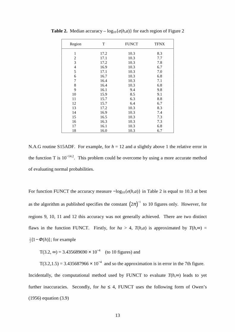
and a straightfoward measure of accuracy is −log10{e(h,a)}, approximately the number of

correct significant figures in T(h,a). Median values of this accuracy measured over a grid of

approximately 200 values of h and a within each of the regions of Figure 2 are given in Table

2 for each of the functions T, FUNCT and TFNX.

The function T is clearly the most accurate. For a ≤ 1 its relative error was always less than

75 times the machine precision (on a VAX 750 with machine precision = 2.78 × 10−17). It is

expected that this relative accuracy of 2.09 × 10−15 (= 10−14.7; i.e. more than 14 significant

figure accuracy) or better will be achieved on machines working as precisely or more

precisely than the VAX 750 but not for machines operating less accurately. For a > 1, and

large values of h, some loss of relative accuracy may be expected due to relative errors in the

13

Table 2. Median accuracy – log10{e(h,a)} for each region of Figure 2

Region T FUNCT TFNX

1 17.2 10.3 8.32 17.1 10.3 7.73 17.2 10.3 7.84 16.9 10.3 6.75 17.1 10.3 7.06 16.7 10.3 6.87 16.4 10.3 7.18 16.4 10.3 6.89 16.1 9.4 9.8

10 15.9 8.5 9.111 15.7 6.3 8.812 15.7 6.4 6.713 17.2 10.3 8.314 16.9 10.3 7.415 16.5 10.3 7.316 16.3 10.3 7.317 16.1 10.3 6.818 16.0 10.3 6.7

N.A.G routine S15ADF. For example, for h = 12 and a slightly above 1 the relative error in

the function T is 10−14.2. This problem could be overcome by using a more accurate method

of evaluating normal probabilities.

For function FUNCT the accuracy measure −log10{e(h,a)} in Table 2 is equal to 10.3 at best

as the algorithm as published specifies the constant ( ) 12 −π to 10 figures only. However, for

regions 9, 10, 11 and 12 this accuracy was not generally achieved. There are two distinct

flaws in the function FUNCT. Firstly, for ha > 4, T(h,a) is approximated by T(h,∞) =

12 [1 ( )]− hΦ ; for example

T(3.2, ∞) = 3.435689690 × 10−4 (to 10 figures) and

T(3.2,1.5) = 3.435687966 × 10−4 and so the approximation is in error in the 7th figure.

Incidentally, the computational method used by FUNCT to evaluate T(h,∞) leads to yet

further inaccuracies. Secondly, for ha ≤ 4, FUNCT uses the following form of Owen’s

(1956) equation (3.9)

14

( ) 1 1( , ) = 2 {tan ( ) ( , )}− − −T h a a S h aπ

with

( )212

2 121

20 1

( 1)( , ) e /2 1

+∞ ∞−

= = +

−=+

∑ ∑j j

ih

j i j

aS h a h i!

j

The term S(h,a) is calculated within FUNCT to the relative accuracy specified by EPS but the

subtraction from tan−1(a) leads to high relative errors in T(h,a) when the relative difference

between tan−1(a) and S(h,a) is small, i.e. when h is large. For example, FUNCT calculates

T(6,0.5) to only seven figure accuracy and T(8.2,0.4) results in purely machine rounding error

on a VAX 750.

For a ≤ 1 and h2(1 + a2) > 0.01, TFNX uses Gaussian quadrature with points and weights

accurate to 7 decimal places and generally achieves a relative accuracy of about 7 significant

figures. For a > 1, equation (2) is implemented with the result that in regions 9, 10 and 11

T(h,a) is evaluated to about 11 figure accuracy and hence the median accuracy over equal

numbers of points with a < 1 and a > 1 given in Table 2 is about 9 figures. As noted by

Young and Minder (1974) more quadrature points will lead to more accuracy (if the points

and weights are specified accurately). This would be the effect of implementing (8) but it

was found that the implementation of T5 with m = 13 (26 point quadrature) in the function T

was computationally more efficient.

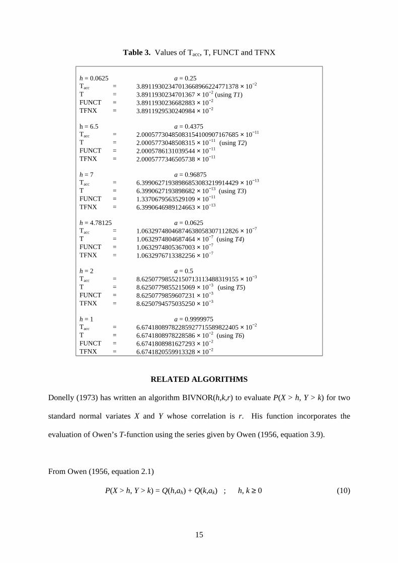
TEST DATA

For six values of h and a, each arising using a different method as determined by Figure 2,

the ‘correct’ value Tacc(h,a) of T(h,a) to 30 figures and the values calculated by the three

functions T, FUNCT and TFNX are given in Table 3.

15

Table 3. Values of Tacc, T, FUNCT and TFNX

h = 0.0625 a = 0.25Tacc = 3.89119302347013668966224771378 × 10−2

T = 3.8911930234701367 × 10−2 (using T1)FUNCT = 3.8911930236682883 × 10−2

TFNX = 3.8911929530240984 × 10−2

h = 6.5 a = 0.4375Tacc = 2.00057730485083154100907167685 × 10−11

T = 2.0005773048508315 × 10−11 (using T2)FUNCT = 2.0005786131039544 × 10−11

TFNX = 2.0005777346505738 × 10−11

h = 7 a = 0.96875Tacc = 6.39906271938986853083219914429 × 10−13

T = 6.3990627193898682 × 10−13 (using T3)FUNCT = 1.3370679563529109 × 10−11

TFNX = 6.3990646989124663 × 10−13

h = 4.78125 a = 0.0625Tacc = 1.06329748046874638058307112826 × 10−7

T = 1.0632974804687464 × 10−7 (using T4)FUNCT = 1.0632974805367003 × 10−7

TFNX = 1.0632976713382256 × 10−7

h = 2 a = 0.5Tacc = 8.62507798552150713113488319155 × 10−3

T = 8.6250779855215069 × 10−3 (using T5)FUNCT = 8.6250779859607231 × 10−3

TFNX = 8.6250794575035250 × 10−3

h = 1 a = 0.9999975Tacc = 6.67418089782285927715589822405 × 10−2

T = 6.6741808978228586 × 10−2 (using T6)FUNCT = 6.6741808981627293 × 10−2

TFNX = 6.6741820559913328 × 10−2

RELATED ALGORITHMS

Donelly (1973) has written an algorithm BIVNOR(h,k,r) to evaluate P(X > h, Y > k) for two

standard normal variates X and Y whose correlation is r. His function incorporates the

evaluation of Owen’s T-function using the series given by Owen (1956, equation 3.9).

From Owen (1956, equation 2.1)

P(X > h, Y > k) = Q(h,ah) + Q(k,ak) ; h, k ≥ 0 (10)

16

where

[ ]12 1 ( ) ( , ) ; 0, 0

( , )0 ; = 0, >0

− − ≥=

h

h

h T h a h > kQ h a

h k

Φ(11)

and

( ) ( )122/ 1= − −ha k h r r ; h > 0.

For h = k = 0,

P(X > 0, Y > 0) = 11 1 sin4 2

−+π

(r).

Care should be taken when computing (11) as, although the function T is accurate to at least

14 significant figures, the subtraction can lead to a loss of relative accuracy in computing Q

and hence in the resultant bivariate normal probability. If, for instance, 1>ha , then using (2),

(11) may be computed as

[ ] [ ]12( , ) ( ,1/ ) ( ) 1 ( )= − − −h h h hQ h a T a h a h a hΦ Φ

where the last term is the product of the two error functions ZNORM1 and ZNORM2. Code

for the functions BIVPRB and Q which evaluate (10) and (11) respectively, is listed after the

code for functions T and TF.

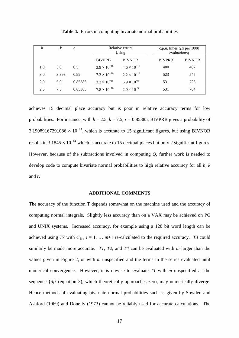
P(X > h, Y > k) was calculated for selected values of h, k (both > 0) and the correlation r

using the function BIVPRB and also using Donelly’s algorithm BIVNOR, both results being

compared with accurate values of the probability calculated to 30 figure accuracy and

presented in Table 4.

Using equation (10) is generally more accurate and slightly faster than BIVNOR, which

17

Table 4. Errors in computing bivariate normal probabilities

h k r Relative errorsUsing

c.p.u. times (µs per 1000evaluations)

BIVPRB BIVNOR BIVPRB BIVNOR

1.0 3.0 0.5 2.9 × 10−18 4.6 × 10−15 400 407

3.0 3.393 0.99 7.3 × 10−16 2.2 × 10−13 523 545

2.0 6.0 0.85385 3.2 × 10−16 6.9 × 10−8 531 725

2.5 7.5 0.85385 7.8 × 10−16 2.0 × 10−3 531 784

achieves 15 decimal place accuracy but is poor in relative accuracy terms for low

probabilities. For instance, with h = 2.5, k = 7.5, r = 0.85385, BIVPRB gives a probability of

3.19089167291086 × 10−14, which is accurate to 15 significant figures, but using BIVNOR

results in 3.1845 × 10−14 which is accurate to 15 decimal places but only 2 significant figures.

However, because of the subtractions involved in computing Q, further work is needed to

develop code to compute bivariate normal probabilities to high relative accuracy for all h, k

and r.

ADDITIONAL COMMENTS

The accuracy of the function T depends somewhat on the machine used and the accuracy of

computing normal integrals. Slightly less accuracy than on a VAX may be achieved on PC

and UNIX systems. Increased accuracy, for example using a 128 bit word length can be

achieved using T7 with C2i , i = 1, … m+1 re-calculated to the required accuracy. T3 could

similarly be made more accurate. T1, T2, and T4 can be evaluated with m larger than the

values given in Figure 2, or with m unspecified and the terms in the series evaluated until

numerical convergence. However, it is unwise to evaluate T1 with m unspecified as the

sequence {dj} (equation 3), which theoretically approaches zero, may numerically diverge.

Hence methods of evaluating bivariate normal probabilities such as given by Sowden and

Ashford (1969) and Donelly (1973) cannot be reliably used for accurate calculations. The

18

problem is overcome at the expense of more computing time by Cooper (1968b) who, in

effect, evaluates 2 jd by

( )212 21

2 22

e /∞−

== ∑

ihj

i j

d h i!

and

( )212

2 1212 1 2 2e /(2 1)

−−− = − − −

jhj jd d h j !

Similarly care should be taken evaluating T2 and T3 as although, for |a| < 1, zi should

approach zero as i increases, numerically the sequence {zi} decreases to near zero and then

diverges for i large.

Increased accuracy can be attained using T5 with large m and the quadrature points and

weights re-calculated to the required accuracy. Accuracy to 30 figures is generally possible

with m = 48. For T2, T3 and T6 and all methods with |a| > 1, standard normal integrals (or

error functions) need to be evaluated with at least the accuracy required in T(h,a).

ACKNOWLEDGEMENT

The authors would like to thank Wolfgang M Hartman for his comments on an earlier version

of this paper.

19

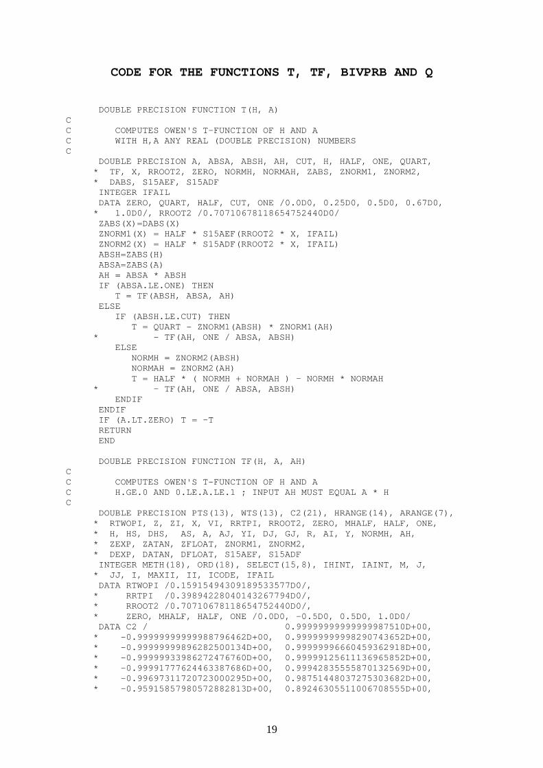
CODE FOR THE FUNCTIONS T, TF, BIVPRB AND Q

DOUBLE PRECISION FUNCTION T(H, A)CC COMPUTES OWEN'S T-FUNCTION OF H AND AC WITH H,A ANY REAL (DOUBLE PRECISION) NUMBERSC DOUBLE PRECISION A, ABSA, ABSH, AH, CUT, H, HALF, ONE, QUART, * TF, X, RROOT2, ZERO, NORMH, NORMAH, ZABS, ZNORM1, ZNORM2, * DABS, S15AEF, S15ADF INTEGER IFAIL DATA ZERO, QUART, HALF, CUT, ONE /0.0D0, 0.25D0, 0.5D0, 0.67D0, * 1.0D0/, RROOT2 /0.70710678118654752440D0/ ZABS(X)=DABS(X) ZNORM1(X) = HALF * S15AEF(RROOT2 * X, IFAIL) ZNORM2(X) = HALF * S15ADF(RROOT2 * X, IFAIL) ABSH=ZABS(H) ABSA=ZABS(A) AH = ABSA * ABSH IF (ABSA.LE.ONE) THEN T = TF(ABSH, ABSA, AH) ELSE IF (ABSH.LE.CUT) THEN T = QUART - ZNORM1(ABSH) * ZNORM1(AH) * - TF(AH, ONE / ABSA, ABSH) ELSE NORMH = ZNORM2(ABSH) NORMAH = ZNORM2(AH) T = HALF * ( NORMH + NORMAH ) - NORMH * NORMAH * - TF(AH, ONE / ABSA, ABSH) ENDIF ENDIF IF (A.LT.ZERO) T = -T RETURN END

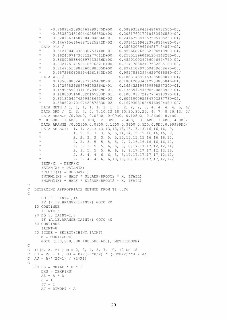
DOUBLE PRECISION FUNCTION TF(H, A, AH)CC COMPUTES OWEN'S T-FUNCTION OF H AND AC H.GE.0 AND 0.LE.A.LE.1 ; INPUT AH MUST EQUAL A * HC DOUBLE PRECISION PTS(13), WTS(13), C2(21), HRANGE(14), ARANGE(7), * RTWOPI, Z, ZI, X, VI, RRTPI, RROOT2, ZERO, MHALF, HALF, ONE, * H, HS, DHS, AS, A, AJ, YI, DJ, GJ, R, AI, Y, NORMH, AH, * ZEXP, ZATAN, ZFLOAT, ZNORM1, ZNORM2, * DEXP, DATAN, DFLOAT, S15AEF, S15ADF INTEGER METH(18), ORD(18), SELECT(15,8), IHINT, IAINT, M, J, * JJ, I, MAXII, II, ICODE, IFAIL DATA RTWOPI /0.15915494309189533577D0/, * RRTPI /0.39894228040143267794D0/, * RROOT2 /0.70710678118654752440D0/, * ZERO, MHALF, HALF, ONE /0.0D0, -0.5D0, 0.5D0, 1.0D0/ DATA C2 / 0.99999999999999987510D+00, * -0.99999999999988796462D+00, 0.99999999998290743652D+00, * -0.99999999896282500134D+00, 0.99999996660459362918D+00, * -0.99999933986272476760D+00, 0.99999125611136965852D+00, * -0.99991777624463387686D+00, 0.99942835555870132569D+00, * -0.99697311720723000295D+00, 0.98751448037275303682D+00, * -0.95915857980572882813D+00, 0.89246305511006708555D+00,

20

* -0.76893425990463999675D+00, 0.58893528468484693250D+00, * -0.38380345160440256652D+00, 0.20317601701045299653D+00, * -0.82813631607004984866D-01, 0.24167984735759576523D-01, * -0.44676566663971825242D-02, 0.39141169402373836468D-03/ DATA PTS / 0.35082039676451715489D-02, * 0.31279042338030753740D-01, 0.85266826283219451090D-01, * 0.16245071730812277011D+00, 0.25851196049125434828D+00, * 0.36807553840697533536D+00, 0.48501092905604697475D+00, * 0.60277514152618576821D+00, 0.71477884217753226516D+00, * 0.81475510988760098605D+00, 0.89711029755948965867D+00, * 0.95723808085944261843D+00, 0.99178832974629703586D+00/ DATA WTS / 0.18831438115323502887D-01, * 0.18567086243977649478D-01, 0.18042093461223385584D-01, * 0.17263829606398753364D-01, 0.16243219975989856730D-01, * 0.14994592034116704829D-01, 0.13535474469662088392D-01, * 0.11886351605820165233D-01, 0.10070377242777431897D-01, * 0.81130545742299586629D-02, 0.60419009528470238773D-02, * 0.38862217010742057883D-02, 0.16793031084546090448D-02/ DATA METH / 1, 1, 1, 1, 1, 1, 1, 1, 2, 2, 2, 3, 4, 4, 4, 4, 5, 6/ DATA ORD / 2, 3, 4, 5, 7,10,12,18,10,20,30,20, 4, 7, 8,20,13, 0/ DATA HRANGE /0.02D0, 0.06D0, 0.09D0, 0.125D0, 0.26D0, 0.4D0, * 0.6D0, 1.6D0, 1.7D0, 2.33D0, 2.4D0, 3.36D0, 3.4D0, 4.8D0/ DATA ARANGE /0.025D0,0.09D0,0.15D0,0.36D0,0.5D0,0.9D0,0.99999D0/ DATA SELECT/ 1, 1, 2,13,13,13,13,13,13,13,13,16,16,16, 9, * 1, 2, 2, 3, 3, 5, 5,14,14,15,15,16,16,16, 9, * 2, 2, 3, 3, 3, 5, 5,15,15,15,15,16,16,16,10, * 2, 2, 3, 5, 5, 5, 5, 7, 7,16,16,16,16,16,10, * 2, 3, 3, 5, 5, 6, 6, 8, 8,17,17,17,12,12,11, * 2, 3, 5, 5, 5, 6, 6, 8, 8,17,17,17,12,12,12, * 2, 3, 4, 4, 6, 6, 8, 8,17,17,17,17,17,12,12, * 2, 3, 4, 4, 6, 6,18,18,18,18,17,17,17,12,12/ ZEXP(X) = DEXP(X) ZATAN(X) = DATAN(X) ZFLOAT(I) = DFLOAT(I) ZNORM1(X) = HALF * S15AEF(RROOT2 * X, IFAIL) ZNORM2(X) = HALF * S15ADF(RROOT2 * X, IFAIL)CC DETERMINE APPROPRIATE METHOD FROM T1...T6C DO 10 IHINT=1,14 IF (H.LE.HRANGE(IHINT)) GOTO 20 10 CONTINUE IHINT=15 20 DO 30 IAINT=1,7 IF (A.LE.ARANGE(IAINT)) GOTO 40 30 CONTINUE IAINT=8 40 ICODE = SELECT(IHINT,IAINT) M = ORD(ICODE) GOTO (100,200,300,400,500,600), METH(ICODE)CC T1(H, A, M) ; M = 2, 3, 4, 5, 7, 10, 12 OR 18C JJ = 2J - 1 ; GJ = EXP(-H*H/2) * (-H*H/2)**J / J!C AJ = A**(2J-1) / (2*PI)C 100 HS = MHALF * H * H DHS = ZEXP(HS) AS = A * A J = 1 JJ = 1 AJ = RTWOPI * A

21

TF = RTWOPI * ZATAN(A) DJ = DHS - ONE GJ = HS * DHS 110 TF = TF + DJ * AJ / ZFLOAT(JJ) IF (J.GE.M) RETURN J = J + 1 JJ = JJ + 2 AJ = AJ * AS DJ = GJ - DJ GJ = GJ * HS / ZFLOAT(J) GOTO 110CC T2(H, A, M) ; M = 10, 20 OR 30C Z = (-1)**(I-1) * ZI ; II = 2I - 1C VI = (-1)**(I-1) * A**(2I-1) * EXP[-(A*H)**2/2] / SQRT(2*PI)C 200 MAXII = M + M + 1 II = 1 TF = ZERO HS = H * H AS = -A * A VI = RRTPI * A * ZEXP(MHALF * AH * AH) Z = ZNORM1(AH) / H Y = ONE / HS 210 TF = TF + Z IF (II.GE.MAXII) GOTO 220 Z = Y * (VI - ZFLOAT(II) * Z) VI = AS * VI II = II + 2 GOTO 210 220 TF = TF * RRTPI * ZEXP (MHALF * HS) RETURNCC T3(H, A, M) ; M = 20C II = 2I - 1C VI = A**(2I-1) * EXP[-(A*H)**2/2] / SQRT(2*PI)C 300 I = 1 II = 1 TF = ZERO HS = H * H AS = A * A VI = RRTPI * A * ZEXP(MHALF * AH * AH) ZI = ZNORM1(AH) / H Y = ONE / HS 310 TF = TF + ZI * C2(I) IF (I.GT.M) GOTO 320 ZI = Y * (ZFLOAT(II) * ZI - VI) VI = AS * VI I = I + 1 II = II + 2 GOTO 310 320 TF = TF * RRTPI * ZEXP(MHALF * HS) RETURNCC T4(H, A, M) ; M = 4, 7, 8 OR 20; II = 2I + 1C AI = A * EXP[-H*H*(1+A*A)/2] * (-A*A)**I / (2*PI)C 400 MAXII = M + M + 1 II = 1 HS = H * H

22

AS = -A * A TF = ZERO AI = RTWOPI * A * ZEXP(MHALF * HS * (ONE - AS)) YI = ONE 410 TF = TF + AI * YI IF (II.GE.MAXII) RETURN II = II + 2 YI = (ONE - HS * YI) / ZFLOAT(II) AI = AI * AS GOTO 410CC T5(H, A, M) ; M = 13C 2M - POINT GAUSSIAN QUADRATUREC 500 TF = ZERO AS = A * A HS = MHALF * H * H DO 510 I = 1 , M R = ONE + AS * PTS(I) 510 TF = TF + WTS(I) * ZEXP(HS * R) / R TF = A * TF RETURNCC T6(H, A); APPROXIMATION FOR A NEAR 1, (A.LE.1)C 600 NORMH = ZNORM2(H) TF = HALF * NORMH * (ONE - NORMH) Y = ONE - A R = ZATAN(Y / (ONE + A)) IF (R.NE.ZERO) TF = TF - RTWOPI * R * ZEXP(MHALF * Y * H * H / R) RETURN END

DOUBLE PRECISION FUNCTION BIVPRB( H, K, R )CC COMPUTES P( X.GT.H, Y.GT.K ) FOR X,Y STANDARD NORMAL WITHC CORRELATION R. H.GE.0 K.GE.0C DOUBLE PRECISION H, K, R, RR, RI, QUART, ZERO, HALF, ONE, X, * Q, RROOT2, RTWOPI, ZNORM2, ZSQRT, ZASIN, DSQRT, DASIN, S15ADF INTEGER IFAIL DATA ZERO, QUART, HALF, ONE /0.0D0, 0.25D0, 0.5D0, 1.0D0/, * RROOT2 /0.70710678118654752440D0/, * RTWOPI /0.15915494309189533577D0/ ZSQRT(X)=DSQRT(X) ZNORM2(X) = HALF * S15ADF(RROOT2 * X, IFAIL) ZASIN(X)=DASIN(X) IF (R.EQ.ZERO) THEN BIVPRB = ZNORM2(H) * ZNORM2(K) ELSE

RR = ONE - R * R IF (RR.GT.ZERO) THEN RI = ONE / ZSQRT(RR) IF (H.GT.ZERO.AND.K.GT.ZERO) THEN BIVPRB = Q (H, (K/H - R) * RI ) + Q (K, (H/K - R) * RI ) ELSEIF (H.GT.ZERO) THEN BIVPRB = Q (H, - R * RI ) ELSEIF (K.GT.ZERO) THEN BIVPRB = Q (K, - R * RI ) ELSE BIVPRB = QUART + RTWOPI * ZASIN(R)

23

ENDIF ELSEIF (R.GE.ONE) THEN IF (H.GE.K) THEN

BIVPRB = ZNORM2(H) ELSE BIVPRB = ZNORM2(K) ENDIF

ELSE BIVPRB = ZERO ENDIF

ENDIF RETURN END

DOUBLE PRECISION FUNCTION Q( H, AH )CC COMPUTES Q = (1/2) * P( Z.GT.H ) - T ( H, AH ) ; H.GT.0C THE RESULT FOR Q IS NON-NEGATIVE.C WARNING : Q IS COMPUTED AS THE DIFFERENCE BETWEEN TWO TERMS;C WHEN THE TWO TERMS ARE OF SIMILAR VALUE THIS MAY PRODUCEC ERROR IN Q.C DOUBLE PRECISION H, AH, AHH, ONE, MINONE, HALF, RROOT2, * X, T, TF, ZNORM1, ZNORM2, S15AEF, S15ADF INTEGER IFAIL DATA HALF, ONE, MINONE /0.5D0, 1.0D0, -1.0D0/, * RROOT2 /0.70710678118654752440D0/ ZNORM1(X) = HALF * S15AEF(RROOT2 * X, IFAIL) ZNORM2(X) = HALF * S15ADF(RROOT2 * X, IFAIL) IF (AH.GT.ONE) THEN

AHH = AH * H Q = TF (AHH, ONE / AH, H) - ZNORM2( AHH ) * ZNORM1 ( H )

ELSE Q = HALF * ZNORM2 ( H ) - T ( H, AH )

ENDIF RETURN END

24

REFERENCES

Abramowitz, M and Stegun, I A (1965). Handbook of mathematical functions. New York:Dover.

Adams, A G (1969). Algorithm 39. Areas under the normal curve. Computer J., 12,197-198.

Borth, D M (1973). A modification of Owen’s method for computing the bi-variate normalintegral. Appl. Statist., 22, 82-85.

Cadwell, J H (1951). The bivariate normal integral. Biometrika, 38, 475-479.

Cooper, B E (1968a). Algorithm AS2. The normal integral. Appl. Statist., 17, 186-187.

Cooper, B E(1968b). Algorithm AS4. An auxiliary function for distribution integrals. Appl.Statist., 17, 190-192. Corrigenda 1969, 18, 118 and 1970, 19, 204.

Cooper, B E (1968c). Algorithm AS5. The integral of the non-central t-distribution. Appl.Statist., 17, 193-194.

Donelly, T G (1973). Algorithm 462. Bivariate normal distribution. Commun. Ass. Comput.Mach., 16, 638.

Hill, I D (1973). Algorithm AS66. The normal integral. Appl. Statist., 22, 424-427.

Hill, I D and Joyce, S A (1967). Algorithm 304. Normal curve integral. Comm. ACM, 10,374-375.

Hornecker, G (1958). Évaluation approachée de la meilleure approximation polynomialed’ordre n de f(x) sur un segment fini (a,b). Chiffres, 1, 157-159.

Kerridge, D F and Cook, G W. (1976). Yet another series for normal integral. Biometrika,63, 401-403.

Numerical Algorithms Group (1997). N A G Fortran Library, Mark 18, Vol 12, Oxford:Numerical Algorithms Group Limited.

Nicholson, C (1943). The probability integral for two variables. Biometrika, 33, 59-72.

Owen, D B (1956). Tables for computing bivariate normal probabilities. Ann. Math. Statist.,27, 1075-1090.

Owen, D B (1959). Tables of the bivariate normal distribution function and related functions,II. Applications of the tables. National Bureau of Standards, Washington D C. NBSAMS 50, XVII-XLII.

Schervish, M H (1984). Multivariate normal probabilities with error bound. Appl. Statist.,33, 81-94.

25

Sowden, R R and Ashford, J R (1969). Computation of the bivariate normal integral. Appl.Statist., 18, 169-180.

Thomas, G E (1986). Remark ASR65. A remark on algorithm AS76: An integral useful incalculating non-central t and bivariate normal probabilities. Appl. Statist., 35, 310-312.

Young, J C and Minder, Ch E (1974). Algorithm AS76. An integral useful in calculatingnon-central t and bivariate normal probabilities. Appl. Statist., 23, 455-457.