Farm work, home work and international productivity ...lanfiles.williams.edu/~dgollin/Papers/RED...

A

l ofaccount

the timeof thee then

rforms

variestimessasts

key1),

Review of Economic Dynamics 7 (2004) 827–850

www.elsevier.com/locate/red

Farm work, home work and internationalproductivity differences

Douglas Gollina, Stephen L. Parenteb, Richard Rogersonc,∗

a Fernald House, Williams College, Williamstown, MA 01267, USAb University of Illinois, 1407 W. Gregory Drive, Urbana, IL 61801, USA

c Department of Economics, College of Business, Arizona State University, Tempe, AZ 85287, US

Received 29 July 2002; revised 30 December 2003

Available online 8 July 2004

Abstract

Agriculture’s share of economic activity is known to vary inversely with a country’s levedevelopment. This paper examines whether extensions of the neoclassical growth model canfor some important sectoral patterns observed in a current cross section of countries and inseries data for currently rich countries. We find that a straightforward agricultural extensionneoclassical growth model fails to account for important aspects of the cross-country data. Wintroduce a version of the growth model with home production, and we show that this model pemuch better. 2004 Elsevier Inc. All rights reserved.

1. Introduction

Economists have long recognized that agriculture’s share of economic activityinversely with the level of output. This is true both across countries and overwithin a given country. Development economists have traditionally viewed the proceof structural transformation—including the relative decline of the agricultural sector—an important feature of the development process.1 In contrast, modern growth theoris

* Corresponding author.E-mail addresses:[email protected] (D. Gollin), [email protected] (S.L. Parente),

[email protected] (R. Rogerson).1 The relevant literature from development economics on structural change is too large to summarize, but

works dealing with the role of agriculture in the process of economic growth include: Johnston and Mellor (196

1094-2025/$ – see front matter 2004 Elsevier Inc. All rights reserved.doi:10.1016/j.red.2004.05.003

828 D. Gollin et al. / Review of Economic Dynamics 7 (2004) 827–850

comes of theeady-, 1994;rch istionalme is

for thes of thessicalationsovidesof theal

tholicymodel

smallsparitytsectors

rowthet al.

uragen.duce

uctionertheory1870–ryat theacrosseriod.

andin

wthral

have tended to abstract from sectoral issues in their examination of international indifferences. A major branch of recent research in this area uses one-sector versionneoclassical growth model to examine the impact of various policy distortions on ststate income levels. (Examples include: Chari et al., 1996; Parente and PrescottPrescott, 1998; and Restuccia and Urrutia, 2001.) A general finding of this reseathat such models can plausibly account for the huge observed disparity in internaincomes provided that the combined share of tangible and intangible capital in incoaround two-thirds.

The purpose of this paper is to determine whether such models can also accountsectoral patterns present in both the cross section of countries and the time seriecurrently rich countries. To accomplish this we consider an extension of the neoclagrowth model to include an agricultural sector and assess the quantitative implicof the theory for both aggregate and sectoral patterns. We believe that this pran additional check on these theories while also offering a careful investigationclaim—central to traditional development economics—that sectoral differences are criticto understanding international income disparities.

Our analysis begins with a straightforward extension of the neoclassical growmodel to include an agricultural sector. Following the literature, we then consider pdifferences across countries that serve to increase the cost of capital. We find that thefails to replicate a key feature of the data first documented by Kuznets (1971) for aset of countries and here for a larger set, namely, the enormous cross-country diin relative productivities of agricultural and non-agricultural sectors. This failure exiswhether we consider distortions that affect the agriculture and non-agriculture sequally or unequally.

This failure leads us to follow Parente et al. (2000) and extend the standard gmodel to incorporate Becker’s model of home production. We deviate from Parenteby incorporating spatial heterogeneity intoour model so that home production possibilitiesdiffer between rural and urban regions. As in Parente et al., distortions that discocapital accumulation move resources out of market activity and into household productioIn our model, however, there is an additional effect. Namely, these distortions inpeople to stay in the rural area, where they devote much of their time to home prodrelative to the urban area. As a result, marketed agricultural output per worker is lowin distorted (poor) economies than in undistorted (rich) economies. To assess ourwe restrict the model’s parameters to roughly match the US observations over the1990 period and then explore the consequences of policy differences for cross countdifferences in income, sectoral compositions, and sectoral productivity. We find thhome production model can account for most of the sectoral differences observedcountries as well as the secular changes in the United States over the 1870–1990 p

Fei and Ranis (1964), Schultz (1964), Lewis (1955), Kuznets (1966), Chenery and Syrquin (1975), JohnstonKilby (1975), Hayami and Ruttan (1985), Mellor (1986), Timmer (1988), and Syrquin (1988). A key debatethis literature is whether agriculture diminishes in importance because it has low inherent potential for gro(e.g., Fei and Ranis, 1964; Lewis, 1955) or because agricultural growth in some way stimulates non-agricultusectors of the economy (e.g., Mellor, 1986).

D. Gollin et al. / Review of Economic Dynamics 7 (2004) 827–850 829

s thatfared outputtill

cludemably be

Moresecularheseces inert pointsdata.ermottces in

mics ofulturalith thee

southern

esay ofes thection 5ction 6

e beginlturaluts or1990

sP

97

5097

As with the home production story told by Parente et al. (2000), our model predictmeasured output differences overstate true differences. For this reason, we compare welbetween distorted and undistorted economies. Despite there being more unmeasurein the distorted economy, the welfare difference between rich and poor countries is slarge.

We certainly are not the first to extend the neoclassical growth model to inan agricultural sector. An early literature dating to Uzawa (1961, 1963), Takaya(1963) and Inada (1963) explored two-sector growth models that could reasonainterpreted as representing an agricultural sector and a non-agricultural sector.recently, Echevarria (1995, 1997) and Kongsamut et al. (1997) have examined thedecline in agriculture’s importance in the currently rich, industrialized nations. Tpapers have not, however, sought to explain the current cross-country differenagriculture’s share of economic activity. In these papers, only initial capital stocks diffacross countries, so that all the cross-sectional observations correspond to differenalong the same equilibrium path. As we document, this view is inconsistent with the

There are a number of other dynamic generalequilibrium models that likewise includan agricultural sector. Glomm (1992), Matsuyama (1992), and Goodfriend and McDe(1995) all take an endogenous growth approach. Laitner (2000) focuses on differensavings patterns across countries. His model conforms to Engels’s Law, but the dynahis model are such that there are extended time periods during which only the agricsector is operating. Caselli and Coleman (2001) focus on a fixed cost associated wacquisition of human capital in order to account for the secular decline of agriculture in thUnited States and the associated convergence in incomes between northern andstates.

Our paper is organized as follows. Section 2 documents the current sectoral differencacross countries and within countries across points in time. Section 3, by wbackground, reviews the standard neoclassical growth model. Section 4 analyzstandard neoclassical growth model extended to include an agriculture sector. Seanalyzes the home production extension of this model with an agricultural sector. Seconcludes the paper.

2. Some development facts

This section documents some key sectoral aspects of the development process. Wwith two well-known facts. The first is that in a cross section of countries, the agricusector is relatively larger in poorer countries, whether measured in terms of outpinputs. Figure 1 plots agriculture’s share of GDP against real GDP per capita, usingdata from the World Bank’sSocial Indicators of Developmentand Penn World Table(PWT 5.6), while Fig. 2 plots agriculture’sshare of total employment against real GDper capita, using 1990 data from the United NationsHuman Development Report 19and PWT 5.6.2 The slope of the trend line fit through the scatter plot in Fig. 1 is−0.094

2 The World Bank’s Social Indicators of Development report agriculture’s share of GDP in 1990 for 1countries in the world. For six more countries, we were able to obtain data on agriculture’s share from the 19


th as 70

re

Fig. 1. Fraction of GPD in agriculture, 1990 cross section.

Fig. 2. Employment in agriculture as fraction of workforce, 1990 cross section.

while the slope of the trend line fit through the scatter plot in Fig. 2 is−0.20. The poorescountries have as much as 50 percent of GDP comprised of agriculture and as muc

United NationsHuman Development Report,and for the United States we used data from the 1997EconomicReport to the President.We then used all of these countries for which 1990 data on real per capita GDP weavailable in the Penn World Tables v. 5.6, leaving us with a total of 102 countries.


s than

henomyg back

Fig. 3. Employment in agriculture as fraction of workforce, time series data for 15 industrial countries.

Fig. 4. Agriculture share of GDP, time series data for 15 industrial countries.

percent of employment in this activity. In the rich countries, these two shares are les10 percent of the totals.

The second well-documented fact is from time series data: the relative size of tagriculture sector both in terms of output and employment declines as an ecodevelops. This is documented in Figs. 3 and 4 using pooled time series data goin


ut and85waslate asso thats

for aare ofultureottedrnlturaltio islture

elativein

),erre taken

Fig. 5. Relative productivity in non-agriculture, by real per capita GDP, 1990 cross section data.

over two centuries for a set of 15 currently rich countries. In these figures the outpemployment shares are plotted against eachcountry’s per capita GDP relative to the 19US level.3 Looking at Fig. 4, for example, agriculture’s share of total employmentabout 50 percent in France in the mid 19th century, and about 50 percent in Italy as1920. During the 20th century, however, these employment shares fell dramaticallyin 1990 they stood at no more than 10 percent in any currently rich country and as little a2 percent in some countries.

The third fact is not as well known, though it is documented in Kuznets (1971)smaller set of countries and an earlier time period. Using the data on agriculture’s shGDP and employment, we compute a measure of output per worker in non-agricrelative to agriculture. Figure 5 displays these relative productivity differences plagainst real GDP per capita for each of the countries in our sample. A striking patteemerges—non-agricultural productivity in poor countries is far higher than agricuproductivity, often by a factor of 10 or more. By contrast, in the rich countries this ratypically less than 2. A regression of relative productivity of non-agriculture to agricuon a constant and log of real GDP per capita yields a slope of−1.9.

It is important to note that these productivity measures are based on domestic rprices. A number of studies have attempted to determine the extent to which differences

3 Data on employment shares and GDP shares in agriculture are taken from Mitchell (1992, pp. 912–917Kurian (1994, pp. 93–94), Mitchell (1993, pp. 775–777), and Mitchell (1995, pp. 1027–1031). Data on real pcapita GDP are taken from Penn World Tables, v. 5.6, for the available years of coverage; historical data afrom Maddison (1995, pp. 194–206).


udies,lative

), anderbycross-asured

aminested inntries.s therelativeallerUnited

relativeivelly thetates,to 2,,ast byple of

ctivity’s richulturalreater

orker initytyes

aggregate

close to

om75)l per

alts fores

domestic relative prices explain these relative productivity differences. One set of stincluding Rao (1993) and Hayami and Ruttan (1985), finds the differences in reproductivities to be at least as large when PPP comparisons are made.4 Another set ofstudies, including Kuznets (1971), Krueger et al. (1992), Schiff and Valdés (1992Bautista and Valdés (1993), finds these differences in relative productivities to be smallon account of agricultural products being systematically under priced in poor countriesas much 40–50 percent. Whichever view we take of relative prices, it is clear that thecountry differences in relative productivity are at least as large as differences in meper capita output.

This striking difference between today’s rich and poor countries leads us to exthe time series data to see whether such large relative productivity differences exithe rich countries a century or so ago when they were as poor as today’s poor couAlthough we do not have time series data for currently rich countries that coverrange of GDP per capita in the cross section, the available data suggests thatproductivity differences in the time series for individual countries are significantly smthan differences in the 1990 cross section. Figure 6 plots the time series data for theStates, United Kingdom, and Canada, along with the 1990 cross section data onsectoral productivity against GDP per capita.5 For the United Kingdom and Canada relatproductivity has been nearly constant over time and close to one. This is essentiacase for almost all the currently rich countries. The one exception is the United Swhich experienced a fairly large drop in this ratio between 1870 and 1900 from 4.3but thereafter maintained a more or less constant ratio of 2.6 As the figure clearly showsa large number of today’s poor countries are far away from the path followed in the ptoday’s rich countries. A similar finding appears in Kuznets (1971) for a smaller samcountries.

The data analysis leads to several obvious questions. Why are relative produdifferences in today’s poor countries so much larger than was the case for todaycountries a century ago, when they had comparable incomes? Why are agricworkers in the poorest countries apparently so unproductive? And why is there not g

4 The Prasada Rao PPP-adjusted data (pp. 135–136, Table 7.3) show that agricultural output per wthe highest-productivity country (New Zealand) is greater than the comparable figure for the lowest-productivcountry (Mozambique) by a factor of 244. The ratio of average productivity in the five highest productivicountries to the average productivity in the five lowestis 139.3! Hayami and Ruttan (1985) also find differencin agricultural output per worker based on PPP measurements to be at least as large than differences inoutput per worker. In the 1960 cross section they find factordifferences in agricultural output per worker betweenthe top five and bottom five countries to be about 30, but in the 1980 cross section the factor difference is50.

5 Data on agriculture’s shares of employment and output for the United Kingdom and Canada are taken frMitchell (1992, 1993); those for the United States aretaken from the US Department of Commerce’s (19Historical Statistics of the United States, and from Kurian (1994) for more recent years. Estimates of reacapita GDP are taken from Maddison (1995) and PWT 5.6.

6 Alston and Hatton (1991) actually suggest that the ratioof 2 for the United States is an artifact of regionproductivity differences and agriculture being concentrated in the South. They show that once one correcnon-cash payments to agricultural workers, there are no differences in agricultural and manufacturing wagwithin US regions.


ss

aper

alnt

at serveerve to

ur

nfinitely

thatsent01)

Fig. 6. Non-agricultural productivityrelative to agricultural productivity—time series contrasted with 1990 crosection.

movement of labor out of agriculture in developing countries? The rest of the pattempts to answer these questions.

3. Background

Recent efforts to account for international income differences within the neoclassicgrowth model have examined the consequencesof cross-country differences in governmepolicies for steady-state income. Two classes of policies have been studied: those thto raise the cost of investment goods relative to consumption goods and those that sdecrease total factor productivity.7 A brief overview of these efforts is instructive for oanalysis.

The standard one-sector neoclassical growth model assumes a representative ilived household with preferences given by

∞∑

t=0

βt log(Ct )

7 Empirical evidence suggests that both of these channels are relevant. Jones (1994) presents evidencethe relative price of equipment is negatively correlated with GDP per capita, and Hall and Jones (1999) preevidence that measured TFP is positively correlated with GDP per capita. See also Restuccia and Urrutia (20and Collins and Williamson (1999) for evidence on the price of capital.


d.

tf the

est of

nmy

o this

priate998;meteresn and

licitlyctoraleraire

hem for

ove,t a

where 0< β < 1 is the discount factor andCt is consumption in periodt . The household isendowed with the economy’s initial capital stock,K0, and one unit of time in each perioA constant returns to scale technology produces output(Yt ) using capital(Kt) and labor(Nt ) according to:

Yt = AKθt

[(1+ γ )tNt

]1−θ,

whereγ is the rate of exogenous technological change andA is a TFP parameter thasummarizes the effects of government policies on a country’s output per unit ocomposite input. Feasibility requires thatCt +Xt � Yt , whereXt is investment in periodt .Capital evolves according toKt+1 = (1 − δ)Kt + Xt/π , whereδ is the depreciation ratand π � 1 summarizes the effect of country-specific policies that increase the coinvestment relative to consumption. Following this literature, we refer toπ as the barrierto capital accumulation.8

In assessing the consequences of differencesin TFP or barriers to capital accumulatiofor differences in output, values forA andπ can be normalized to one for the US econowithout loss of generality. If another country has policesthat yield TFP parameterA andbarrierπ it is easy to show that steady state output of the United States relative tcountry is given byA−1/(1−θ)πθ/(1−θ).

This theory can generate large differences in output per capita given approcombinations of values forA, π , andθ . A number of researchers (see e.g., Prescott, 1Parente and Prescott, 2000) have argued that a value of two thirds for the share paraθ

is reasonable. This argument is based on a broadinterpretation of capital that encompassboth tangible and intangible varieties. In what follows we adopt this parameterizatiointerpretation of capital.

4. The neoclassical growth model with agriculture

In this section we extend the standard neoclassical growth model to expincorporate an agricultural sector, and ask whether it can account for the sedevelopment facts described previously if policy distortions are present. The numfor this economy is the manufactured good.

4.1. Model economy

Instantaneous utility is now defined over two consumption goods. To account for tsecular decline in agriculture’s share of economic activity we adopt a functional forpreferences of the Stone–Geary variety. The discounted stream of utility is thus

∞∑

t=0

βt[log(Ct ) + φ log(at − a)

], (1)

8 While it is clearly important to understand how specific policies are mapped intoA andπ , we think thisreduced-form approach serves to better highlight the keyelements of our subsequent analysis. As noted abwe do not adhere to a literal interpretation ofπ as a policy distortion; the variable could equally well reflecvariety of institutional differences across economies.


ctionslwork.

nt the

ulturefor

arlier,we do

sr, and

or thelem is

ardless

heg

r main

tors.non-

where φ is a preference parameter,at is consumption of the agricultural good,Ct isconsumption of the manufactured good, anda > 0 is the subsistence term.9

The agricultural sector produces output (Yat ) using capital (Kat) and labor (Nat) asinputs according to theCobb–Douglastechnology:10

Yat = AaKθaat

[(1+ γ )tNat

]1−θa . (2)

The manufacturing sector produces output (Ymt ) using capital (Kmt) and labor (Nmt) asinputs according to theCobb–Douglastechnology:

Ymt = AmKθmmt

[(1+ γ )tNmt

]1−θm. (3)

As we note later in this section, the assumption of Cobb–Douglas production funhas important substantive consequences for our analysis.11 In addition to being a naturastarting point for an analysis of this sort, this assumption is supported by empirical(See, for example, the cross-country analysis of Hayami and Ruttan, 1985.)

Output from the manufacturing sector can be used for consumption or to augmetwo capital stocks. The manufacturing resource constraint is thus,Ct + Xmt + Xat � Ymt .Output from the agriculture sector can only be used for consumption so the agricresource constraint is simplyat � Yat . Capital is sector-specific, so the laws of motionthe two stocks of capital in the economy are:

Kmt+1 = (1− δ)Kmt + Xmt/πm, (4)

Kat+1 = (1− δ)Kat + Xat/πa. (5)

For simplicity we assume that both capital stocks depreciate at a common rate; thisrestriction is not important to our findings. Given the sectoral patterns documented eit seems potentially important to allow for policies that may differ across sectors, soallow policy to have differential effects on the accumulation of eachcapital stock throughsector specific barriersπa andπm.

The household is endowed with one unit oftime in each period, which it allocatebetween working in the manufacturing sector and working in the agricultural sectowith the economy’s initial capital stocks,Ka0 andKm0.

4.2. Quantitative findings

It is not necessary to calibrate the model to determine whether it can account frelative sectoral differences observed across countries. It cannot. The main probthat the model predicts that relative productivity is the same across countries reg

9 Following a longstanding convention in the literature, we refer to the non-agricultural sector as tmanufacturing sector, although in our empirical work we will interpret this sector to include manufacturinactivity as well as other industrial activities and services.

10 We abstract from land as a fixed factor in agriculture. Adding land to the model does not affect ouquantitative findings.

11 Note that we assume here that exogenous technologicalchange occurs at the same rate in the two secThis assumption is motivated by the lack of any discernible trend in the relative price of agriculture toagriculture goods in the United States over the last 100 years (see Kongsamut et al., 1997).


lrethat

mee

wardral

e suchpedeavily

nsiderivities

ant tovedpslative

or.blecapitalto ahere,weens), we

eenncludetioned

ultureectorality

es,d in the

of policy differences reflected in TFP or barriers to capital accumulation.12 The reasonfor this is as follows. Because labor is perfectlymobile between sectors, the agriculturawage rate and the non-agricultural real wagerate are equal in equilibrium. As factors apaid their marginal products, profit maximization by firms in both sectors impliesθa = waNa/paYa andθm = wmNm/pmYm. Sincewa = wm and capital shares are the saacross countries, it follows that relative productivity in each country is just the ratio of thcapital shares, i.e.,

paYa/Na

Ym/Nm= θm

θa. (6)

Policy distortions, therefore, have no effect on relative productivity. The straightforagricultural extension of the neo-classicalgrowth model cannot account for the sectorelative productivity differences observed across countries.

The failure of the model suggests a number of possible alternative theories. Onalternative in the spirit of Caselli and Coleman (2001) is to allow for factors that imthe movement of labor from agriculture into manufacturing. Some countries do herestrict movement out of rural areas. We do not follow this approach. Instead, we coan extension of the neoclassical growth model that allows for home production actthat differ between rural and urban sectors.

As noted earlier, the assumption of Cobb–Douglas production functions is importthis analytic result. This raises the issue of to what extent one could generate the obserdifferences in relative productivities by having a different production function. Perhanot surprisingly, it is possible to account for some of the observed differences in reproductivities by moving to a different specification of technology in the agricultural sectIntuitively, if a poor country has less capital and labor and capital are more substitutain agriculture than in non-agriculture, then as the amount of capital decreases theto labor ratio may fall more in agriculture than in non-agriculture, thereby leadinglower average product of labor in agriculture. While we do not present the detailscalculations that we performed showed that with an elasticity of substitution betcapital and labor in agriculture of two (rather than one for the case of Cobb–Douglacould plausibly account for one half of the differences in relative productivities betwthe richest and poorest countries given the observed differences in capital. We cothat theoretically there is scope for such an explanation to play a role, though as menearlier, empirical work supports the assumption of a unitary elasticity of substitution.

5. The model with agriculture and home production

In this section, we add a home production sector to the growth model with agricand examine whether it can account for the US secular growth facts and the sdevelopment facts. The key feature of our abstraction is to allow for spatial heterogene

12 To examine whether the model can account for the sectoral transformation undergone by the rich countrione would need to calibrate the model. The performance of this model along this dimension is discussenext section.


s thanleadr thanapping

ity byn then

tion

nuumilyal.of thernden the

arketital tome

arerences,

non-en

omertime

ruraln

kesns.

and have a rural region that is more conducive to home production opportunitiethe urban region. With no loss in generality, we focus on policy differences thatto differences in the cost of investment goods relative to consumption goods rathedifferences in TFP. As shown by Parente and Prescott (2000), there is a one-to-one mfrom this type of distortion to TFP.

5.1. Model economy

The critical aspect of our formulation is that we incorporate spatial heterogenehaving an urban region and a rural region. Agriculture takes place exclusively irural region, whereas manufacturing is assumed to take place exclusively in the urbaregion.13 Individuals living in both regions are assumed to have access to home productechnologies that differ across regions.

To simplify the analysis, we assume that the economy is populated with a contiof identical infinitely lived families, with each family consisting of a continuum of fammembers. Families, rather than individual family members, own the economy’s capitThis assumption buys us considerable simplicity since we do not have to keep trackheterogeneity in capital holdings associatedwith differences in location. A family membelives either in the rural area, in which case he divides his time between the home sector athe agricultural sector, or in the urban area, in which case he divides his time betwehome sector and the manufacturing sector. A family head makes all the family decisions—how many family members live in each region, how they allocate their time between mand home production, how much consumption each receives and how much capaccumulate. In keeping with the analysis of the previous section, we continue to assuperfect mobility of individuals across locations.

For reasons of space, we describe only those aspects of the model economy thatassociated with the introduction of home production and spatial heterogeneity. Prefeare the same as before and given by Eq. (1). However, non-agriculture consumptionCt , isnow a CES aggregator of the manufacturing goodcmt , and the home good,cht ,

Ct = [µc

ρmt + (1− µ)c

ρht

]1/ρ. (7)

In (7), the parameterµ reflects the relative importance of the home and marketagriculture goods and the parameterρ determines the elasticity of substitution betwehome-produced and market-produced goods.

With the introduction of home production, the capital endowment includes rural hcapital and urban home capital denoted byKR0, andKU0. Each individual family membeis still endowed with one unit of time each period. Individuals must divide theirbetween market and home production in each period. For workers located in theregion this constraint is writtennat + nRt = 1, while for workers located in the urbaregion it is writtennmt + nUt = 1.

13 Of course this is a stylization. In reality, a considerable amount of non-agricultural market production taplace in rural areas. Moreover, urban agriculture (e.g., poultry and swine) may be important in some locatioNonetheless, the stylization is convenient here.


. Withon

tiesbeuction

e that

oingtocks

pital, butt haveark.

ng

ose

anndeas.as, andia

The technologies for the manufacturing and agricultural sectors are as beforethe addition of home production in the spatial model, there are two home productitechnologies,

Yjt = AjKαjt

[(1+ γ )tNjt

]1−α, (8)

where Kjt is capital, andNjt is hours in home production in regionj = U,R. Animportant feature of our specification is that we assume that home production opportuniare “better” in the rural sector than in the urbansector. There are various ways this couldmodeled; we choose to incorporate this feature by assuming that the two home prodtechnologies are identical except for a difference in TFP. Specifically, we assumAR > AU .14

Investment in home capital, like investment in market capital, requires forgconsumption of the manufactured good. The laws of motion for the home capital sare:

KRt+1 = (1− δ)KRt + XRt , (9)

KUt+1 = (1− δ)KUt + XUt . (10)

As is apparent, home capital is assumed to depreciate at the same rate as market cathe policy distortions do not affect home capital. Relaxing these assumptions do noa large impact on our findings, but in any case we view this as a reasonable benchm

The family head’s objective is to maximize the discounted value of average utilityacross family members. Letλt denote the fraction of the representative family liviin the urban region at datet . Additionally, let U(c

jmt , c

jht , a

jt ) denote the period utility

of a family member who lives in regionj and receives the datet consumptionallocation(c

jmt , c

jht , a

jt ). The problem of the head of the representative family is to cho

a sequence{(ajt , c

jmt , c

jht )j=U,R,Kmt+1,Kat+1,KUt+1,KRt+1, nmt , nat , nUt , nRt , λt }∞t=0

that maximizes:∞∑

t=0

βt[λtU

(cUmt , c

Uht , a

Ut

) + (1− λt )U(cRmt , c

Rht , a

Rt

)](11)

subject to:

∞∑

t=0

Pt

[λt

(cUmt + pata

Ut

) + (1− λt )(cRmt + pata

Rt

) − πmKmt+1 − πaKat+1

− KUt+1 − KRt+1]

14 Alternatives include assuming that the rural home production function is less capital intensive than the urbhome production function, or that there are complementarities in time inputs between agricultural activities ahome production, or that there are better substitution possibilities between home and market goods in rural arFor example, child care may be more easily supplied while working in rural areas than in urban areservices such as food processing and distribution are accomplished via home production in rural areas, and vmarket production in urban areas.


int,teing infamilyegion.

fromturinge hometraded.

e.g.,this

amilyption

home

rmineacross

sothpolicy

regate

andard.seere is

isby the

�∞∑

t=0

Pt

[wmtλtnmt + rmtKmt + (1− λt )watnAt + ratKAt

+ (1− δ)(πmKmt + πaKat + KRt + KUt)], (12)

nat + nRt = 1, (13)

nmt + nUt = 1, (14)

λt cUht � AUK

αu

Ut

[(1+ γ )tλtnUt

]1−αu, (15)

(1− λt )cRht � ARK

αR

Rt

[(1+ γ )t (1− λt )nRt

]1−αR , (16)

given initial capital stocks.15 Equation (12) is the family’s intertemporal budget constrawhere Pt is the Arrow–Debreu date 0 price of the manufacturing good at dat .Equations (13) and (14) are the time use constraints of individual family members livthe rural and urban regions. Equation (15) states that home consumption of ruralmembers is less than or equal to the total home production produced in that rEquation (16) is the analogous constraint for the urban population.

In our abstraction there are two features that distinguish home productionmanufacturing sector output. First, capital can only be produced in the manufacsector. One possible variation is to assume that home capital can be produced in thsector, though we have not explored it. Second, home produced output cannot beIn some instances we think of this as a defining characteristic of home production—child care is home produced only if the family provides it for itself. In other cases,assumption is probably not appropriate—for example, clothing made at home by fmembers in the rural area may be sent to family members in the city. While our assumis extreme, what is important for our results is that a significant component ofproduction cannot easily be transferred across regions.

5.2. Quantitative findings

In this section we examine the quantitative properties of the model in order to detewhether it can account for the sectoral differences observed across countries andtime within a given country. We proceed by firstrestricting the model’s parametersthat its equilibrium path over a 120-year period roughly matches the US economy’s paover the 1870–1990 period. For this parameterized economy, we then examine howdistortions affect the model’s predictions for differences across countries in aggincome and sectoral patterns of production.

5.2.1. CalibrationThere are three aspects of the model that make the calibration procedure non-st

The first is that capital is interpreted broadly to include intangible capital. Becauinvestments in intangible capital are not measured in the national accounts, th

15 The fact that the family chooses the division of individuals between the urban and rural areas means that thproblem is not concave. However, it can still be shown that the solution to this problem is characterizedusual first order conditions. See Rogerson (1984) for a proof in a similar context.


tnt ofarente

is thewsectoronly

ecomesstant.estingof theecline.

equire

le this

Homeed as armineis lackome

tionson, the

seriesuction.xploithome

eholdlture,

Rupert

ent ins plusisof thelue of

nt,

tialinus

and 4).seholdtside

a discrepancy between output in the model and output in theNational Income and ProducAccounts(NIPA). This necessitates that we adjust output in the model by the amouthis unmeasured investment in order to make comparisons with the NIPA data. (See Pand Prescott, 2000 for an extended discussion.)

The second aspect of the model that makes the calibration non-standardsubsistence term in the utilityfunction. This term implies that we can no longer viethe US economy as if it were on a constant growth path, as is the case in the oneversion of the model described in Section 3. In this version, the economy willapproach a constant growth path equilibrium as the effect of the subsistence term binfinitesimally small, or equivalently, as agriculture’s share of GDP approaches a conIn reality, this share has declined rather substantially over the postwar period, suggthat the postwar period should not be viewed as a constant growth path. In termscalibration, this means that the parameter values must be restricted to match this dIt follows that we cannot assign the technology growth rate parameterγ to be the averaggrowth rate of US GDP per capita over the postwar period. However, we can still rethat the model match the growth rate of US GDP per capita over some interval. Whimatch is not solely determined by the value ofγ , it will be heavily influenced by it.

The third aspect that makes the calibration non-standard is home production.production is unmeasured in the NIPA. The stock of household durables can be usrough estimate for the total stock of home capital. However, there is no way to detehow much of this is allocated between rural households and urban households. Thof measurement implies that it will not be possible to restrict all the values of the hproduction preference and technology parameters with the use of data. Some assumpwill have to be made to restrict a number of these parameter values. For this reascalibration should be viewed as somewhat exploratory in nature.

The basic strategy of the calibration is to use observations from the US timeto restrict all the preference and technology parameters not related to home prodThe one exception is the value of the capital share in manufacturing. For this we ethe estimate of intangible capital’s share from Parente and Prescott (2000). For theproduction parameters, our strategy is to use information on the stock of housdurables in the United States, market hours data for individuals outside of agricuand estimates for the elasticity of substitution between market and home goods byet al. (1995) and McGrattan et al. (1997).

The empirical counterparts of the model are as follows. Total (measured) investmmarket capital is the sum of residential and non-residential investment expenditure25 percent of government expenditures. The remaining part of government expendituresconsidered to be consumption. The value of agricultural output is the value of outputfarm sector, and the value of (measured) nonagricultural output is GDP less the vafarm output. The source of these statistics is the1991 Economic Report of the PresideTables B1, B8, and B32 and the US Commerce Department’sHistorical Statistics ofthe United States(1975), Series F 251. Agricultural capital is simply non-residenfarm capital. Measured non-agricultural physical capital is simply total capital magricultural capital. The source of the capital stock data is Musgrave (1993, Tables 2The empirical counterparts relevant for home production are the 1990 stock of houdurables, and the fraction of discretionary time spent in market work for individuals ou


f bother than

thers so thehangesks forme

aswthrateath.very

nt toment,ltural

GDP,

erpartses fortions.odel

s about

itherr than

ceare ofent ofates

orkers

someyond a

this

is

the agricultural sector. We note that the empirical counterparts of the residences ofarmers and non-farmers are included as part of the manufactured capital stock, rathas part of household capital.

A final issue in the calibration is the choice of values for initial capital stocks. Rathan attempt to obtain estimates of capital stocks for 1870, we choose these valueimplied series for investment and sectoral labor shares do not display any abrupt cin the periods following 1870. Loosely speaking, the idea is to choose capital stoc1870 that would be consistent with the economy being on a transition path that began soyears earlier.16

Table 1 reports the parameter values and provides comments on how each value wchosen. Note thatγ = 0.0198, which is slightly lower than the 2 percent average grorate over 1960–1990 thatwe targeted in our calibration. This is because the growthduring this period is still slightly higher than its value on the constant growth pNonetheless, the behavior of the calibrated model in the post World War II period issimilar to a constant growth equilibrium; the capital to output ratios, the investmeoutput ratio, and the growth rate of real GDP are all nearly constant. As a final comour procedure for allocating the two-thirds share for total capital in the nonagricusector yields a split of 0.19 for tangible capital and 0.48 for intangible capital.17 Thisimplies that in 1990, investment in intangible capital is around one-half of measuredwhich is in line with the estimates suggested by Parente and Prescott (2000).18

5.2.2. Properties of the calibrated model5.2.2.1. The United States, 1870–1990.At this stage, it is informative to examine somof the long run properties of the calibrated model and compare them with their countein the data. As we calibrate the model to reproduce the beginning and ending valuagriculture’s share of GDP in the United States, we trivially match these observaHowever, with respect to the rate of decline in agriculture’s share of GDP, the mmatches the US experience reasonably well with the exception of some large swingtrend in the 1890–1930 period.

We did not explicitly calibrate to match agriculture’s share of employment, in e1870 or 1990. In the United States in 1870, agriculture’s share of employment is largeits share of output. The calibrated model also displays this property, though the differenis not as large as in the data. Specifically, the model predicts an employment sh36 percent in 1870 versus the value of 48 percent found in the data (US DepartmCommerce, 1975).19 The 48 percent share found in the data most surely overestimagriculture’s share of employment in 1870 as there are a large number of part time w

16 Given that our model is in discrete time, this procedure really only restricts initial capital stocks to lie ininterval. However, since the different values in this interval do not have any effect on the equilibrium befew periods this does not appear to be a serious issue.

17 This split is relevant because of the need to do the GNP accounts excluding intangible investments.18 Note that we assume intangible capital only in the manufacturing sector. We discuss the importance of

later in the paper.19 The calibrated non-home production model studiedin Section 4 actually performs worse along th

dimension.


000)le

ndver

ut

e

US

ock

6.5

e

less

and

and

and

rs inmodel

ctiv-ctivityis ratiocon-ts thatver theodel

is ac-ate of7.5 to

Table 1Parameter values

Parameters Value Comments

θm Capital share in manufacturing 0.667 Based on estimates from Parente and Prescott (2for market production with tangible and intangibcapital.

θa Capital share in agriculture 0.240 Consistent with 1990 agricultural capital stock aoutput, and average annual rate of interest opostwar period.

Am TFP in manufacturing 1.00 Normalization that only affects units in which outpis measured.

Aa TFP in agriculture 1.00 Normalization that only affects level of relativprices.

πm Barrier in manufacturing 1.00 Normalization for same reasons above.πa Barrier in agriculture 1.00 Normalization for same reasons above.γ Exogenous rate of technological

change0.198 Consistent with average annual growth rate of

over postwar period of 2 percentδ Depreciation rate 0.063 Consistent with 1990 investment and capital st

data.β Discount factor 0.960 Consistent with average annual interest rate of

percent over postwar period.φ Expenditure share 0.003 1990 agriculture’s share of output of 2.3 percent.a Subsistence term 0.393 1870 agriculture’s share of output of 22 percent.AR TFP in rural home production 1.00 Normalization that only affects units in which hom

good is measured.AU TFP in urban home production 0.900 Assumption that home production in urban area is

efficient compared to rural area by 10 percent.α Capital share in home production 0.110 Consistent with stock of household durables

market work outside of agriculture in 1990.µ Share parameter between market

and home goods0.362 Consistent with stock of household durables

market work outside of agriculture in 1990.ρ Elasticity of substitution between

market and home goods0.400 Based on micro estimates of Rupert et al. (1995)

McGrattan et al. (1997) for United States.

in US agriculture, and these workers are not distinguished from full time workeconstructing employment measures. In light of this, the discrepancy between theand the data along this dimension is not as bad as it appears.

Next we turn to the model’s predictions for the behavior of relative sectoral produities and prices over time. The model predicts that the ratio of average labor produin the two sectors is very nearly constant and equal to one. For the United States, thwas roughly constant only after 1920 and closer to two. This is not particularly discerting, since as documented earlier, the work by Alston and Hatton (1991) suggesthe data overstate the true differences in 1920. For relative prices, the changes o120-year period are quite small. In particular, the relative price of agriculture in the mis effectively constant, changing by roughly 1 percent over the 120-year period. Thcords well with the data (see, e.g., Kongsamut et al., 1997). Additionally, the real rreturn for the calibrated economy shows this same small decline, decreasing from6.5 percent over the 120-year period.


ourlrbant anek in0 andkweeklls byrk,

onoores ononomy

m

to bothvenlyat

rkt

e,

sharector,oss theivity isut per

ed

P perbarrierntries.ted

nomy,my itsectoralost

1990.

The model has rich predictions for time allocations. Not surprisingly, givenassumptions about home production possibilities, we find that individuals in the ruraregion devote more of their time to home production than do workers in the uregion. More interesting, our model predicts a decline in the fraction of time thaindividual spends in market work over the 120-year period. The decline in the workwemanufacturing is more than 10 percent, and virtually all of it takes place between 1871960. Hence, this model can account for a large part of the secular decline in the worin manufacturing. In the agricultural sector the decline is even larger: the workweek faalmost 25 percent. Coincident with this secular decrease in time devoted to market wothere is a large movement of workers from the rural to the urban region.

5.2.2.2. Cross-country comparisons.How does the introduction of home productipossibilities affect the model’s predictionsfor sectoral differences across rich and pcountries? We now use this model to examine the implications of distortionary policithe development process. To do this we contrast the behavior of our calibrated ecwith no distortions to another economy with barriers,πa � 1 andπm � 1. As above, weassume that initial capital stocks in the distorted economy are such that the equilibriupaths for other variables display no abrupt changes over the 120-year period.

We have studied three cases. The first assumes that the distortions apply equallycapital stocks and result in a fourfold increase in the cost of both types of capital relatito the undistorted economy (i.e.,πm = πa = 4). The second assumes that distortions oapply to the manufacturing capital stock (i.e.,πm = 4,πa = 1). The third case assumes thdistortions only apply to the agriculture capital stock (i.e.,πm = 1,πa = 4). Table 2 reportsour results. For expositional purposes, we report only the results from the benchmaeconomy, (i.e.,πm = πa = 1), and the case withπm = πa = 4. The reason for this is thathe results for theπm = 1 andπa = 4 case are practically identical to the benchmark casand the results for theπm = 4 andπa = 1 case are practically identical to theπm = πa = 4case.

Table 2 reports NIPA GDP per capita, agriculture’s share of GDP, agriculture’sof employment, relative productivity, time allocated to agriculture work in the rural seand time allocated to market work in the manufacturing sector at various dates acrundistorted and distorted economies. We note that our measure of relative productchosen to correspond to the concept used in the data. Specifically, it looks at outpworker and not output per unit of labor input. Additionally, we note that GDP is calculatby using a geometric average of the 1990 price of agriculture in the two economies.

As the table shows, the model with home production generates differences in GDcapita as observed in the data. The difference in GDP per capita associated with aof 4 is approximately the factor 30 observed across the richest and poorest couThe model also predicts sizeable differences in the share of employment accounfor by agriculture across rich and poor countries in 1990. In the undistorted ecoagriculture’s share of employment is 5 percent in 1990, while in the distorted econoshare is 63 percent. Third, the model generates large cross-country differences in srelative productivity. Relative productivity of the agricultural sector in the model is almsix times larger in the undistorted economy than it is in the distorted economy in


in the

is thate richy are

a richunced.to the

andchangecular

tortedgion,in the

g. Overglyotingrs inn overnt

over,

ather. The. Onere somall

ce oftionsonss

ws atplying

Table 2International comparisons

GDP paYa/GDP 1− λ ym/ya na nm

π = 1 π = 4 π = 1 π = 4 π = 1 π = 4 π = 1 π = 4 π = 1 π = 4 π = 1 π = 4

1870 1.00 0.12 0.22 0.68 0.36 0.83 1.90 2.32 0.58 0.68 0.64 0.701900 1.92 0.14 0.13 0.49 0.22 0.74 2.03 2.97 0.52 0.42 0.60 0.511930 3.91 0.18 0.07 0.32 0.14 0.67 2.13 4.36 0.48 0.26 0.57 0.431960 7.31 0.27 0.04 0.19 0.08 0.63 2.20 7.36 0.46 0.16 0.55 0.401990 13.4 0.41 0.02 0.12 0.05 0.63 2.26 12.9 0.44 0.09 0.55 0.39

This is also very close to the difference between the richest and poorest countries1990 cross section.

The reason the model generates these large differences in relative productivitythere are large differences in time allocations of rural workers in 1990 across th(undistorted) and poor (distorted) economies. Rural workers in the poor economworking only about 20 percent as much in market activity as their counterparts ineconomy. Differences in time allocations in the urban region are much less pronoThis asymmetry between the distortions on rural and urban time allocations is dueasymmetry of home production opportunities across rural and urban regions.

As can be seen in the table, relative productivity differentials across distortedundistorted countries increase over time. This phenomenon is driven by the secularin time allocations of workers in the two regions. In the distorted economy the sedecline in the (market) workweek in the rural region is much larger than in the undiseconomy. Initially, although the distorted economy has more workers in the rural reworkers in the distorted economy have roughly the same time allocations as workersundistorted economy. This is because the subsistence constraint is relatively bindintime, this constraint eases and the time allocation in the rural area becomes increasindistorted toward home production. Although the table stops in 1990 it is worth nthat the time allocation of rural workers to market production in subsequent yeathe distorted economy continues to show a decline, although at a slower rate thathe 1870–1990 period. In the undistorted economy, in contrast, there is no subsequedecline. As a result, the relative productivity differentials continue to widen. Morethese differentials begin to reflect real output differences in agriculture.

The one dimension of the data on which the performance of the model is rdisappointing is agriculture’s share of output across rich and poor countriesdifferences predicted by the model are small relative to what is found in the datareason why the differences in agriculture’s share of output implied by the model asmall is that individuals living in the rural region in the distorted economy allocate a sfraction of their time to market activities. A second reason is that the relative priagriculture is lower in the poorer country, by roughly 80 percent. Alternative specificafor preferences may give rise to smaller effects on relative prices and help the modelthis dimension. Accounting for the large difference in agriculture’s share of GDP acrorich and poor countries is a matter for future work.

A rather surprising result is that measured output in the distorted economy groa much slower rate than in the undistorted economy over the 120-year period, im


t untilrate ofatternrnritiesTheseneed totl withelying foralf of

an inercentre oflts tondmpute90

segelarge

es.eases.lsoectics ofwe are

that relative GDPs diverge for a long time. In fact, as the table documents, it is noroughly the end of the sample period that the distorted economy displays a growthreal GDP that is roughly equal to the exogenous growth rate of technology. This pis not generated in the other models studiedin this paper. It is, however, the patteobserved in the data. With the start of the Industrial Revolution in England, dispain living standards between the world’s rich and poor countries began to increase.disparities continued to increase until 1950. Our research shows that one does notassume differential rates of exogenous technological change or poverty traps to accounfor this pattern. Instead, a two-sector version of the neoclassical growth modehome production, a broad concept of capital,and a subsistence term can qualitativgenerate this pattern. We conclude that this model may be very useful in accountthe divergence in international incomes from the Industrial Revolution to the latter hthe twentieth century.

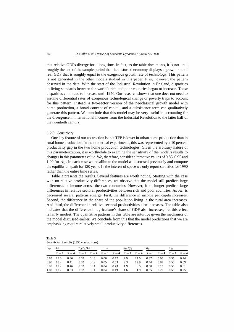
5.2.3. SensitivityOne key feature of our abstraction is that TFP is lower in urban home production th

rural home production. In the numerical experiments, this was represented by a 10 pproductivity gap in the two home production technologies. Given the arbitrary natuthis parameterization, it is worthwhile to examine the sensitivity of the model’s resuchanges in this parameter value. We, therefore, consider alternative values of 0.85, 0.95 a1.00 forAU . In each case we recalibrate the model as discussed previously and cothe equilibrium path for 120 years. In the interest of space we only report statistics for 19rather than the entire time series.

Table 3 presents the results. Several features are worth noting. Starting with the cawith no relative productivity differences, we observe that the model still predicts lardifferences in income across the two economies. However, it no longer predictsdifferences in relative sectoral productivities between rich and poor countries. AsAU isdecreased several patterns emerge. First, the difference in income per capita increasSecond, the difference in the share of the population living in the rural area incrAnd third, the difference in relative sectoralproductivities also increases. The table aindicates that the difference in agriculture’s share of GDP also increases, but this effis fairly modest. The qualitative patterns in this table are intuitive given the mechanthe model discussed earlier. We conclude from this that the model predictions thatemphasizing require relatively small productivity differences.

Table 3Sensitivity of results (1990 comparisons)

AU GDP paYa/GDP 1− λ ym/ya na nm

π = 1 π = 4 π = 1 π = 4 π = 1 π = 4 π = 1 π = 4 π = 1 π = 4 π = 1 π = 4

0.85 13.3 0.36 0.02 0.13 0.06 0.72 2.9 17.5 0.37 0.08 0.55 0.440.90 13.4 0.41 0.02 0.12 0.05 0.63 2.3 12.9 0.44 0.09 0.55 0.390.95 13.2 0.46 0.02 0.11 0.04 0.43 1.9 6.5 0.50 0.13 0.55 0.311.00 13.2 0.53 0.02 0.11 0.04 0.19 1.6 1.9 0.55 0.27 0.55 0.25


levantwelling inrencenalyzedsumefactorrencesrt,und ins

ly thatn well-sumestorted

mucheasuregrowthotone

ds withivein our

gerif

th thismy

eachtis our

tor ofmberhe twooutputs.tes

t matter

A second issue noted earlier was our assumption that intangible capital is only rein the manufacturing sector. This assumption is quantitatively significant. As isknown, the impact of a given barrier on cross-country income differences is increasthe capital share. Moreover, the impact of home production is increasing in the diffebetween the capital share in the home sector and the market sector. We have also aa version of the model in which we abstract from intangible capital completely and asa capital share of 0.30 in the manufacturing sector. Not surprisingly, in this case thedifference in aggregate output as of 1990 is 2.25 rather than 30, and the factor diffein relative productivities is 1.7 rather than 5. Obviously, as is true in all models of this sowith a smaller capital share one needs larger distortions to match the differences fothe data. The key point here is that we get a sizeable elasticity of relative productivitiewith respect to changes in aggregate income even with the smaller capital share.

5.2.4. Welfare comparisonAs discussed and analyzed in Parente et al. (2000), home production models imp

differences in measured income across countries overstate the true differences ibeing. For our calibrated model, we note that in 1990, the undistorted economy conroughly 33 times more of the manufactured consumption good than does the diseconomy, 1.1 times more of the agricultural good, but only about two-thirds ashome produced output. In what follows we use our model to give a more precise mof actual welfare differences and contrast them to those obtained in the standardmodel described in Section 3. We note that our measure is not affected by montransformations of the utility function.20

For the standard growth model, we assume a parameterization that roughly accorthe values used in Section 5. The barrierπ is selected so that the factor difference in relatsteady state incomes in this model equals the factor difference of 33 we obtainedbenchmark specification for 1990. Given a capital share equal to 2/3, the correspondinvalue of π is 5.75. We compute the welfare gain associated with removing the barrifor this economy as follows. First, we compute the equilibrium path that would resultan economy beginning in the steady state corresponding toπ = 5.75 were to eliminatethis barrier. Next, we compute the utility of the representative agent associated wiequilibrium path. We then compute the utilityof the representative agent if the econodoes not eliminate this barrier and it remains in the steady state corresponding toπ = 5.75.We then determine the factor by which we would have to increase consumption inperiod under this second scenario in order that the resulting lifetime utility equal thaachieved when the barrier were removed. This factor increase in consumptionwelfare measure.

The number we obtain is 2.8; i.e., if consumption were to be increased by a fac2.8 the individual would be indifferent about removing the barrier. Note that this nuis small in comparison to the differences in steady state consumptions. The ratio of tconsumptions across the two steady states is 33—the same as the ratio of the twoThe fact that our compensating differential is so much smaller than this factor indica

20 Note that we have also assumed that there is unmeasured investment in the economy. This will nofor our welfare calculations since they are based on consumption flows.


y

omenstor bytionrs is

of them this

poorlarge.

shareplieder, we

ationsensiond poorhome

areas.plusber of

section

r theirEUDCof theat the

rsityd ofwhilepport

the importance of allowing for the accumulation of capital needed toreach the new steadstate.

We now repeat this calculation in the context of our two-sector growth model with hproduction. Because there is no steady state for this economy, we take the 1990 allocatioin the distorted economy as our stating point in the exercise. In determining the facwhich consumption would have to be increased in each period, we assume the consumpof the home good, manufacturing good, and agricultural good of all family membeincreased proportionately. The number we obtain is 1.9, which is about two-thirdsnumber we obtained in the welfare calculation for standard model. We conclude frothat while home production does diminish the welfare differences between rich andcountries for a given difference in measured output, the reduction is not particularly

6. Conclusion

Development economists have long noted the importance of agriculture in theof economic activity in poor countries. Contemporary researchers working with apgeneral equilibrium models almost always abstract from sectoral issues. In this papintroduced agriculture into the neoclassical growth model and examined the implicfor international incomes and sectoral patterns. We found that a straightforward extof the model fails to account for key sectoral differences observed across rich ancountries. This failure led us to consider an extension of the model that incorporatesproduction. The key implication of this model is that distortions tocapital accumulationlead to a relative increase in the amount of unmeasured activity taking place in ruralA reduction of the distortions leads to an efficiency-enhancing reallocation of inputsan increase in measured economic activity. We found the model accounts for a numfeatures of the sectoral transformation observed in economic data, both in the crossand the time series.

Acknowledgments

We thank Lee Alston, Bob Evenson, Ed Prescott and an anonymous referee focomments. We have also benefitted from the comments of participants at the 1998 Nmeetings; the 1999 Econometric Society winter meetings; and the 1999 meetingsSociety for Economic Dynamics. Versions of this paper were presented at seminarsFederal Reserve Bank of Minneapolis, the University of California at Davis, Univeof Illinois, University of Pennsylvania, Yale University, Purdue University, the BoarGovernors, and Williams College. All errors are our own. Part of this work was doneGollin was visiting the Economic Growth Center at Yale. Rogerson acknowledges sufrom the NSF.

We thank Stephanie Sewell for helpful research assistance.


nal

ingte,

ion.

er

–1950.

of

ic

. Irwin,

.rs?

iv.

mic

nomic

te-

82.82.

am,

is.l of

old

nt

k.w

References

Alston, L., Hatton, T., 1991. The earnings gap between agricultural and manufacturing laborers, 1925–41. Jourof Economic History 51 (March), 83–99.

Bautista, R., Valdés, A., 1993. The Bias Against Agriculture: Trade and Macroeconomic Policies in DevelopCountries. International Center for Economic Growth and the International Food Policy Research InstituSan Francisco, with ICS Press.

Caselli, F., Coleman II, J.W., 2001. The US structural transformation and regional convergence: a reinterpretatJournal of Political Economy 109 (3), 584–616.

Chari, V.V., Kehoe, P., McGrattan, E. 1996. The poverty of nations: a quantitative exploration. Working pap5414. NBER.

Chenery, H.B., Syrquin, M., 1975. Patterns of Development, 1950–1970. Oxford Univ. Press, London.Collins, W., Williamson, J. 1999. Capital goods prices, global capital markets and accumulation: 1870

Working paper No. 7145. NBER.Echevvaria, C., 1995. Agricultural development vs. industrialization: effects of trade. Canadian Journal

Economics 28 (3), 631–647.Echevarria, C., 1997. Changes in sectoral composition associated with economic growth. International Econom

Review 38 (2), 431–452.Fei, J.C.H., Ranis, G., 1964. Development of the Labor Surplus Economy: Theory and Policy. Richard D

Homewood, IL. A publication of the Economic Growth Center, Yale University.Glomm, G., 1992. A model of growth and migration. Canadian Journal of Economics 42 (4), 901–922.Goodfriend, M., McDermott, J., 1995. Early development. American Economics Review 85 (1), 901–922Hall, R.E., Jones, C.I., 1999. Why do some countries produce so much more output per worker than othe

Quarterly Journal of Economics 114 (1), 83–116.Hayami, Y., Ruttan, V.W., 1985. Agricultural Development: An International Perspective. Johns Hopkins Un

Press, Baltimore.Inada, K., 1963. On a two-sector model of economic growth: comments and a generalization. Review of Econo

Studies 30 (June), 95–104.Johnston, B.F., Mellor, J.W., 1961. The role of agriculture in economic development. American Eco

Review 51 (4), 566–593.Johnston, B.F., Kilby, P., 1975. Agriculture and Structural Transformation: Economic Strategies in La

Developing Countries. Oxford Univ. Press, New York.Jones, C.I., 1994. Economic growth and the relative price of capital. Journal of Monetary Economics 34, 359–3Kongsamut, P., Rebelo, S., Xie, D., 1997. Beyond balanced growth. Review of Economic Studies 68 (4), 869–8Krueger, A.O., Schiff, M., Valdés, A., 1992. The PoliticalEconomy of Agricultural Pricing Policy, vols. I–III. A

World Bank, Baltimore. Comparative study. Published for the World Bank by Johns Hopkins Univ. Press.Kurian, G.T., 1994. Datapedia of the United States 1790–2000: America Year by Year. Bernan Press, Lanh

MD.Kuznets, S., 1966. Modern Economic Growth. Yale Univ. Press, New Haven.Kuznets, S., 1971. Economic Growth of Nations. Harvard Univ. Press, Cambridge, MA.Laitner, J., 2000. Structural change and economic growth. Review of Economic Studies 67, 545–561.Lewis, A., 1955. Theory of Economic Growth. Allen Unwin, London.Maddison, A., 1995. Monitoring the World Economy: 1820–1992. Development Centre of the OECD, ParMatsuyama, K., 1992. Agricultural productivity, comparative advantage, and economic growth. Journa

Economic Theory 58 (2), 317–334.McGrattan, E., Rogerson, R., Wright, R., 1997. An equilibrium model of the business cycle with househ

production and fiscal policy. International Economic Review 38, 267–290.Mellor, J.W., 1986. Agriculture on the road to industrialization. In: Lewis, J.P., Kallab, V. (Eds.), Developme

Studies Reconsidered. Overseas Development Council, Washington, DC.Mitchell, B.R., 1992. International Historical Statistics: Europe 1750–1988. Stockton Press, New York.Mitchell, B.R., 1993. International Historical Statistics: The Americas 1750–1988. Stockton Press, New YorMitchell, B.R., 1995. International Historical Statistics: Africa, Asia & Oceania1750–1988. Stockton Press, Ne

York.


and

cal

the

5–

nd

93–

ls.

f therld

k

view of

.),

eau

Musgrave, J., 1993. Fixed reproducible tangible wealth inthe United States: Revised estimates for 1990–92summary estimates for 1925–92. Survey of Current Business (September), 61–69.

Parente, S., Prescott, E.C., 1994. Barriers to technology adoption and development. Journal of PolitiEconomy 102 (2), 298–321.

Parente, S., Prescott, E.C., 2000. Barriers to Riches. MIT Press, Cambridge.Parente, S.L., Rogerson, R., Wright, R., 2000. Homeworkin development economics: home production and

wealth of nations. Journal of Political Economy 108, 680–687.Prescott, E.C., 1998. Needed: a theory of total factor productivity. International Economic Review 39 (3), 52

551.Rao, P., 1993. Intercountry comparisons of agricultural output and productivity. Paper 112. FAO Economic a

Social Development, Rome. Food and Agriculture Organization of the United Nations.Restuccia, D., Urrutia, C., 2001. Relative prices and investment rates. Journal of Monetary Economics 47,

122.Rogerson, R., 1984. Topics in the theory of labor markets. Unpublished PhD dissertation. Univ. of Minnesota.Rupert, P., Rogerson, R., Wright, R., 1995. Estimating substitution elasticities in household production mode

Economic Theory 6 (1), 179–193.Schiff, M., Valdés, A., 1992. The Political Economy of Agricultural Pricing Policy, vol. 4: A Synthesis o

Economics in Developing Countries. A World Bank, Baltimore. Comparative study. Published for the WoBank by Johns Hopkins Univ. Press.

Schultz, T.W., 1964. Transforming Traditional Agriculture. Yale Univ. Press, New Haven.Syrquin, M., 1988. Patterns of structural change. Chapter 7 in: Chenery, H., Srinivasan, T.N. (Eds.), Handboo

of Development Economics, vol. I. Elsevier Science, Amsterdam.Takayama, A., 1963. On a two-sector model of economic growth: a comparative static analysis. Re

Economic Studies 30, 95–104.Timmer, C.P., 1988. The agricultural transformation.Chapter 8 in: Chenery, H., Srinivasan, T.N. (Eds

Handbook of Development Economics, vol.I. Elsevier Science, Amsterdam.US Department of Commerce, 1975. Historical Statistics of the United States: Colonial Times to 1970. US Bur

of the Census, Washington, DC.Uzawa, H., 1961. On a two-sector model of economic growth: I. Review of Economic Studies 29, 40–47.Uzawa, H., 1963. On a two-sector model of economic growth: II. Review of Economic Studies 30, 105–118.

Farm work, home work and international productivity ...lanfiles.williams.edu/~dgollin/Papers/RED...

Documents

Transcript of Farm work, home work and international productivity ...lanfiles.williams.edu/~dgollin/Papers/RED...