Farfield Plume Measurement and Analysis on the NASA 300M and
28
The 33st International Electric Propulsion Conference, The George Washington University, USA October 6 – 10, 2013 1 Farfield Plume Measurement and Analysis on the NASA-300M and NASA-300MS IEPC-2013-057 Presented at the 33rd International Electric Propulsion Conference, The George Washington University • Washington, D.C. • USA October 6 – 10, 2013 Wensheng Huang * , Rohit Shastry † , George C. Soulas ‡ , and Hani Kamhawi § National Aeronautics and Space Administration Glenn Research Center, Cleveland, Ohio, 44135, USA NASA is developing a 10- to 15-kW Hall thruster system to support future NASA missions. This activity is funded under the Space Technology Mission Directorate Solar Electric Propulsion Technology Demonstration Mission project. As a part of the development process, the NASA-300M, a 20-kW Hall thruster, was modified to incorporate the magnetic shielding concept and named the NASA-300MS. This activity was undertaken to assess the viability of using the magnetic shielding concept on a high-power Hall thruster to greatly reduce discharge channel erosion. This paper reports on the study to characterize the far-field plumes of the NASA-300M and NASA-300MS. Diagnostics deployed included a polarly-swept Faraday probe, a Wien filter (ExB probe), a retarding potential analyzer, and a Langmuir probe. During the study, a new, more accurate, integration method for analyzing Wien filter probe data was implemented and effect of secondary electron emission on the Faraday probe data was treated. Comparison of the diagnostic results from the two thrusters showed that the magnetically shielded version performed with ~2% higher voltage utilization efficiency, ~2% lower plume divergence efficiency, and ~2% lower mass utilization efficiency compared to the baseline version. The net change in efficiency is within the aggregate measurement uncertainty so the overall performance is roughly equal for the two versions of the thruster. Anode efficiency calculated from thrust stand measurement corroborates this finding. Abbreviations and Nomenclature * Research Engineer, Propulsion and Propellants, [email protected]. † Research Engineer, Propulsion and Propellants, [email protected]. ‡ Research Engineer, Propulsion and Propellants, [email protected]. § Research Engineer, Propulsion and Propellants, [email protected]. GRC = Glenn Research Center HEFT = Human Exploration Framework Team STMD = Space Technology Mission Directorate AFRL = Air Force Research Laboratory LEO = Low Earth Orbit GEO = Geosynchronous Earth Orbit 300M = NASA-300M 300MS = NASA-300MS 300MS-2 = NASA-300MS configuration 2 RPA = Retarding Potential Analyzer CEX = Charge-exchange SEE = Secondary Electron Emission MCD = Mean Channel Diameter a = Anode efficiency v = Voltage utilization efficiency d = Divergence efficiency b = Current utilization efficiency m = Mass utilization efficiency q = Charge utilization efficiency
Transcript of Farfield Plume Measurement and Analysis on the NASA 300M and
The 33st International Electric Propulsion Conference, The George Washington University, USA
October 6 – 10, 2013
1
Farfield Plume Measurement and Analysis on
the NASA-300M and NASA-300MS
IEPC-2013-057
Presented at the 33rd International Electric Propulsion Conference,
The George Washington University • Washington, D.C. • USA
October 6 – 10, 2013
Wensheng Huang*, Rohit Shastry
†, George C. Soulas
‡, and Hani Kamhawi
§
National Aeronautics and Space Administration Glenn Research Center, Cleveland, Ohio, 44135, USA
NASA is developing a 10- to 15-kW Hall thruster system to support future NASA
missions. This activity is funded under the Space Technology Mission Directorate Solar
Electric Propulsion Technology Demonstration Mission project. As a part of the
development process, the NASA-300M, a 20-kW Hall thruster, was modified to incorporate
the magnetic shielding concept and named the NASA-300MS. This activity was undertaken
to assess the viability of using the magnetic shielding concept on a high-power Hall thruster
to greatly reduce discharge channel erosion. This paper reports on the study to characterize
the far-field plumes of the NASA-300M and NASA-300MS. Diagnostics deployed included a
polarly-swept Faraday probe, a Wien filter (ExB probe), a retarding potential analyzer, and
a Langmuir probe. During the study, a new, more accurate, integration method for
analyzing Wien filter probe data was implemented and effect of secondary electron emission
on the Faraday probe data was treated. Comparison of the diagnostic results from the two
thrusters showed that the magnetically shielded version performed with ~2% higher voltage
utilization efficiency, ~2% lower plume divergence efficiency, and ~2% lower mass
utilization efficiency compared to the baseline version. The net change in efficiency is within
the aggregate measurement uncertainty so the overall performance is roughly equal for the
two versions of the thruster. Anode efficiency calculated from thrust stand measurement
corroborates this finding.
Abbreviations and Nomenclature
* Research Engineer, Propulsion and Propellants, [email protected].
† Research Engineer, Propulsion and Propellants, [email protected].
‡ Research Engineer, Propulsion and Propellants, [email protected].
§ Research Engineer, Propulsion and Propellants, [email protected].
GRC = Glenn Research Center
HEFT = Human Exploration Framework
Team
STMD = Space Technology Mission Directorate
AFRL = Air Force Research Laboratory
LEO = Low Earth Orbit
GEO = Geosynchronous Earth Orbit
300M = NASA-300M
300MS = NASA-300MS
300MS-2 = NASA-300MS configuration 2
RPA = Retarding Potential Analyzer
CEX = Charge-exchange
SEE = Secondary Electron Emission
MCD = Mean Channel Diameter
a = Anode efficiency
v = Voltage utilization efficiency
d = Divergence efficiency
b = Current utilization efficiency
m = Mass utilization efficiency
q = Charge utilization efficiency
The 33st International Electric Propulsion Conference, The George Washington University, USA
October 6 – 10, 2013
2
I. Introduction
N 2010, NASA established the Human Exploration Framework Team (HEFT) to analyze exploration and
technology concepts and provided inputs to the agency's senior leadership on the key components of a safe,
sustainable, affordable, and credible future human space exploration endeavor for the nation.1 The team concluded,
in part, that the use of a high power (i.e. on the order of 300 kW) solar electric propulsion system could significantly
reduce the number of heavy lift launch vehicles required for a human mission to a near earth asteroid.1, 2
Hall
thrusters were found to be ideal for such applications because of their high power processing capabilities and their
efficient operation at moderate specific impulses, which leads to reduced trip times that are necessary for such
missions.2-4
Recent electric propulsion system model estimates that considered factors such as cost, mass, fault-
tolerance, cost uncertainty, complexity, ground test vacuum facility limitations, previously demonstrated power
capabilities, and possible technology limitations have shown that Hall thrusters operating at power levels of 20-50
kW are strong candidates for human exploration missions operating at total powers up to 500 kW.2, 5
As an intermediate step towards the aforementioned higher power Hall thruster system, the Space Technology
Mission Directorate (STMD) is investing in the development of a 10- to 15-kW Hall thruster. The NASA Glenn
Research Center (GRC) is partnering with the Jet Propulsion Laboratory (JPL) to carry out this development work.
The aforementioned thruster will serve as a stepping stone to higher power and provide a state-of-the-art propulsion
system for the Solar Electric Propulsion Technology Demonstration Mission (SEP TDM). SEP TDM, initially
announced in 2011, is aimed at demonstrating new cutting edge technology in flexible solar arrays, spacecraft bus,
and electric propulsion that will increase the maturity of these SEP technologies for future commercial and
government uses. Once these technologies have been demonstrated, they are expected to enable higher performance
LEO to GEO transfers as well as a number of other near-Earth orbit transfers and station-keeping maneuvers. These
technologies may also benefit a potential robotic mission to redirect an asteroid into cis-lunar orbit for crew
exploration. In longer terms, these technologies will reduce mission costs for NASA interplanetary robotic missions
in general, and will serve as a precursor to higher power systems for human interplanetary exploration.
The magnetic shielding (MS) concept, recently developed by JPL, has the potential to greatly reduce discharge
channel wall erosion, which is a dominant life-limiting mechanism for traditional Hall thrusters.6 This concept
greatly benefits Hall thruster technology development and was previously demonstrated on a 6-kW Hall thruster.7, 8
To mitigate possible risks of applying the MS concept to higher power thrusters, NASA GRC and JPL took a
combined experimental and modeling approach to study the application of the MS concept on the 20-kW NASA-
300M. The NASA-300M was developed from 2004 to 2005 for project Prometheus but was not tested until recently
due to project cancellation.9 With the recent renewal in interest towards high-power Hall thrusters, the performance
of the NASA-300M was characterized in 2010.9 The risk mitigation activities began with the modification of the
NASA-300M into a magnetically-shielded version of the same thruster, called the NASA-300MS. A series of
experiments and simulations were then performed to characterize the difference in behavior between the NASA-
300M and the NASA-300MS. For a general overview of the MS modification, the system performance, and the
simulation work, please see Kamhawi’s paper.10
For a description of the wall and interior Langmuir probe studies,
please see Shastry’s paper.11
This paper will focus on the plume characterization study and the accompanying
efficiency analysis.
The plume characterization study involved the use of a number of far-field diagnostics to study various plume
characteristics of the NASA-300M and NASA-300MS. Measurements from these diagnostics can then be used to
infer the effectiveness with which various performance-driving processes are carried out in the thrusters. Each of
these processes is assigned an efficiency factor in a phenomenological efficiency model. By comparing the trends in
the efficiency factors between the two thrusters, one can determine how applying the MS concept changes thruster
performance and which performance-driving processes are the drivers. For this study, a far-field Faraday probe was
swept in a polar fashion to map the ion current density. A Wien filter, also known as an ExB probe, a retarding
potential analyzer (RPA), and a Langmuir probe were mounted at a fixed location on the thruster axis in the far-field
plume. The ExB probe, so called because of the orthogonal electric and magnetic fields inside the probe, was used to
measure the species fractions of the various charged states of xenon. The RPA and the Langmuir probe were used to
measure the energy per charge of the exhaust plume.
The main focus of this paper will be on the comparison of the efficiency analyses between the NASA-300M and
NASA-300MS. This paper will also cover comparison between the NASA-300MS and NASA-300MS-2, which is
the same as the NASA-300MS except with a shortened discharge channel. Other topics that will be covered include
a new, more accurate, method of integration for analyzing ExB probe data and the effect of secondary electron
emission on Faraday probe data.
I

The 33st International Electric Propulsion Conference, The George Washington University, USA
October 6 – 10, 2013
3
The paper begins by describing the efficiency model used in the present study in Sec.II, followed by a
description of the experiments in Sec.III. Next, the paper will describe data analyses and individual probe results for
the RPA (Sec.IV), the ExB probe (Sec.V), and the Faraday probe (Sec.VI). Then, the paper presents the overall
efficiency analyses and comparison between the 300M and 300MS, as well as the 300MS and 300MS-2, in Sec. VII.
The paper ends with the conclusions in Sec.VIII. Appendices attached after Sec.VIII give the derivation of the new
integration method for analyzing ExB data.
II. Background
The purpose of the present study is to determine what effects the application of the MS concept has on the
performance of a high-power Hall thruster. The performance of a Hall thruster is typically measured by its anode
efficiency, defined in Eq. (1).
dda
2
aVIm2
Tη
(1)
In this equation, T is thrust, ma is anode mass flow rate, Id is discharge current, and Vd is discharge voltage.
However, the anode efficiency alone does not provide information about the plasma generation and acceleration
processes that drive the performance of the thruster.
A phenomenological efficiency model is a way of breaking down and describing various physical phenomena
that affect the overall efficiency of a Hall thruster. The purpose of a phenomenological efficiency model is to help
researchers quantify the trends in the processes that drive the overall thruster efficiency. Many efficiency models
have been proposed for the Hall thruster in the past. The complexity of these models depended on the operating
environment and the state of knowledge in the community at the time. The model used in this paper is the same as a
prior work by Shastry,12
which has evolved over time from a number of other studies.13-16
The model is shown in Eq.
(2) to (7).
qmbdva (2)
d
RPAv
V
V
(3)
2d )(cos
(4)
d
bb
I
I
(5)
k k
kmm
a
bXem
Z,
em
Im
(6)
k
kk
2
k
kk
qZ/
Z/
(7)
Where a, the anode efficiency, is the same as that calculated from Eq. (1), v is the voltage utilization efficiency, d
is the divergence efficiency, b is current utilization efficiency, m is the mass utilization efficiency, q is the charge
utilization efficiency, VRPA is the ion energy per charge, δ is the charged-weighted divergence angle, the Ib is the
total beam current, mXe is the mass of xenon, e is the elementary charge constant, m is the part of mass utilization
efficiency that depends on charge state information, Ωk is the current fraction of the k-th species, and Zk is the
charge of the k-th species.
The voltage utilization efficiency describes, on the average, how much of the voltage provided by the discharge
supply is actually used to accelerate the ions. This factor is typically measured by the RPA.
The divergence efficiency describes how much of the kinetic energy imparted to the ions is axial, thrust-
producing, kinetic energy. This factor is typically measured by the Faraday probe.
The 33st International Electric Propulsion Conference, The George Washington University, USA
October 6 – 10, 2013
4
The current utilization efficiency describes how much of the discharge current is carried by ions instead of
electrons. Electrons generate negligible thrust compared to the ions. This factor is typically measured by the Faraday
probe.
The mass utilization efficiency describes how much of the mass flow exiting the thruster channel is in the form
of ions. This factor typically requires data from the Faraday probe and the ExB probe.
The charge utilization efficiency is a number of terms representing the effects of having multiply-charged
species that are not already described by the other terms in the efficiency model.
III. Experimental Setup
For the sake of brevity and to simplify plot labeling, NASA-300M will sometimes be referred to as the 300M in
this paper. Similarly, 300MS is NASA-300MS and 300MS-2 is NASA-300MS-2. Operating conditions are labeled
as www V, yy kW, where www is the discharge voltage in volts and yy is the discharge power in kilowatts. Unless
otherwise noted, all spatial positions presented in this paper have been normalized by the mean channel diameter of
the thrusters, which is identical for all three variants. The mean channel diameter (MCD) is defined as the average of
the inner and outer discharge-channel wall diameters.
A. Thrusters and Test Matrices
The NASA-300M is a magnetic-layer Hall thruster. It was designed based on the principles outlined in
Manzella’s dissertation work.17
This thruster was originally developed for high-specific-impulse missions9 and has
lens-type magnetic field topology.18, 19
For this paper, the magnetic field settings of the 300M were optimized to
give a shape roughly symmetric about the channel centerline while maximizing the anode efficiency. The NASA-
300MS is a magnetically-shielded Hall thruster created from the NASA-300M. The magnetic circuit of the thruster
was modified to achieve the MS topology while retaining most of the original 300M thruster. As such, the physical
dimensions of the 300MS are nearly identical to that of the 300M. The biggest differences in the exterior of the two
thrusters are the presence of chamfers on the downstream edge of the discharge channel walls. The physics-based
modeling program Hall2De was used to validate the design of the magnetic field topology of the 300MS. For more
details about the modifications needed to apply the MS concept and the modeling work, see Kamhawi’s paper.10
Experimental verification of the plasma potentials and electron temperatures at the channel walls was also
performed and detailed in Shastry’s paper.11
For this paper, the magnetic field settings of the 300MS were set to
maintain the MS topology while maximizing the anode efficiency. Both thrusters were operated with the same
centrally-mounted hollow cathode, which was derived from the discharge cathode for NASA’s Evolutionary Xenon
Thruster (NEXT).9 The cathode flow fraction was 8%. Figures 1 and 2 show photographs of the NASA-300M and
NASA-300MS, respectively.
The NASA-300MS-2 is a second configuration of the NASA-300MS with a shortened discharge channel. The
modification was achieved by moving the anode downstream so that the channel length is roughly 20% shorter. This
configuration was made to investigate whether the thruster could be made more compact to decrease mass without
impacting the performance and magnetic shielding. The data will be used to guide the design of the 10- to 15-kW
thruster. Comparisons will be made between the 300M and the 300MS to study the effect of applying magnetic
shielding, and between the 300MS and the 300MS-2 to study the effect of shortening the discharge channel.
The nominal operating condition of NASA-300M and NASA-300MS is 500 V, 20 kW. For the purpose of
comparing the thruster versions, eight operating conditions have been identified as reference points. These eight
Figure 1. The NASA-300M on a thrust stand.
Figure 2. The NASA-300MS on a thrust stand.
The 33st International Electric Propulsion Conference, The George Washington University, USA
October 6 – 10, 2013
5
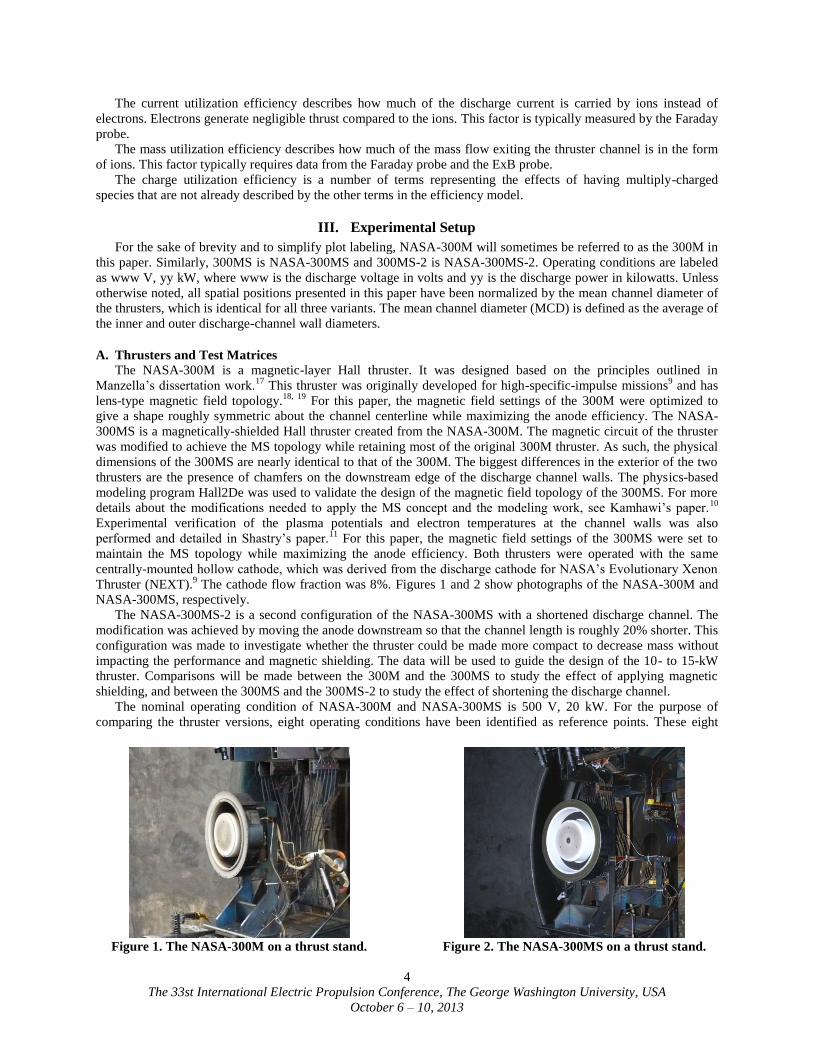
conditions span discharge voltages from 300 to 500 V,
discharge currents from 20 to 50 A, and discharge powers
from 10 to 20 kW. The thrusters operated with anode
efficiencies of 65 to 70% over these eight conditions. Figure
3 shows the combined test matrix for the thruster versions.
Reference points are highlighted by red circles and will be the
main focus of the paper. Data from non-reference conditions
will be used to supplement plots about trends within
individual thruster versions. The boron nitride channel walls
of the 300M have accumulated <110 hours of operation time
prior to the start of this study. The boron nitride channel walls
of the 300MS were freshly manufactured for this study.
The test campaign for the 300MS and 300MS-2 was
spread over three tests. Test 1 was the performance and
plume characterization test on the 300MS. Test 2 was the same but on the 300MS-2. Test 3 was the interior plasma
characterization test on the 300MS. At the end of test 1, the boron nitride channel has seen 49 hours of operation. At
the end of test 2, the channel has seen 82 hours of operation. At the end of test 3, the channel has seen 99 hours of
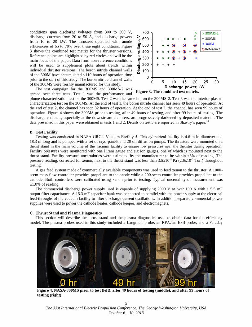
operation. Figure 4 shows the 300MS prior to testing, after 49 hours of testing, and after 99 hours of testing. The
discharge channels, especially at the downstream chamfers, are progressively darkened by deposited material. The
data presented in this paper were obtained in tests 1 and 2. Details on test 3 are reported in Shastry’s paper.11
B. Test Facility
Testing was conducted in NASA GRC’s Vacuum Facility 5. This cylindrical facility is 4.6 m in diameter and
18.3 m long and is pumped with a set of cryo-panels and 20 oil diffusion pumps. The thrusters were mounted on a
thrust stand in the main volume of the vacuum facility to ensure low pressures near the thruster during operation.
Facility pressures were monitored with one Pirani gauge and six ion gauges, one of which is mounted next to the
thrust stand. Facility pressure uncertainties were estimated by the manufacturer to be within ±6% of reading. The
pressure reading, corrected for xenon, next to the thrust stand was less than 3.5x10⁻³
Pa (2.6x10⁻⁵
Torr) throughout
testing.
A gas feed system made of commercially available components was used to feed xenon to the thruster. A 1000-
sccm mass flow controller provides propellant to the anode while a 200-sccm controller provides propellant to the
cathode. Both controllers were calibrated using xenon prior to testing. Typical uncertainty of measurement was
±1.0% of reading.
The commercial discharge power supply used is capable of supplying 2000 V at over 100 A with a 5.5 mF
output filter capacitance. A 15.3 mF capacitor bank was connected in parallel with the power supply at the electrical
feed-throughs of the vacuum facility to filter discharge current oscillations. In addition, separate commercial power
supplies were used to power the cathode heater, cathode keeper, and electromagnets.
C. Thrust Stand and Plasma Diagnostics
This section will describe the thrust stand and the plasma diagnostics used to obtain data for the efficiency
model. The plasma probes used in this study included a Langmuir probe, an RPA, an ExB probe, and a Faraday
Figure 3. The combined test matrix.
Figure 4. NASA-300MS prior to test (left), after 49 hours of testing (middle), and after 99 hours of
testing (right).

The 33st International Electric Propulsion Conference, The George Washington University, USA
October 6 – 10, 2013
6
probe. Unless otherwise stated, all probe biases were applied with commercial power supplies.
The thrust stand used in this study is an inverted pendulum thrust stand designed by Haag.20
It is actively cooled
during operation. The nominal accuracy of this thrust stand is ±2%.9 Long-term thermal drift is corrected by
measuring the thrust signal with all gas flow to the thruster off and then assuming a linear change in the zero-thrust
value over time. The maximum thermal drift was found to be ~10 mN.
A Langmuir probe, an RPA, and an ExB probe were mounted to a probe tower with accompanying shielding and
shutters protecting the RPA and the ExB probe. This farfield probe tower was attached to a vertical motion stage
located ~27 MCD downstream of the thruster exit plane and sitting behind a body shield. During the data acquisition
process, each probe was moved vertically to a point roughly along the central axis of the thruster before
measurements were taken. The probe tower retreated behind the shield once data acquisition was completed. Figure
5 shows a photograph of the diagnostics setup. Figure 6 shows a photograph of the farfield probe tower. A farfield
Faraday probe was mounted onto a commercially available three-axis belt-driven motion system. The motion system
provides 2D rectilinear motion and probe rotation. Positioning accuracy is ~1 mm and <0.1°, respectively.
For the test of the 300M, the Langmuir probe consists of a single tungsten wire protruding from an alumina tube.
This probe was used to obtain the plasma potential at the same location as the RPA so that the RPA data can be
corrected by this potential. For the tests of the 300MS, a disk probe was used to improve data fidelity. The Langmuir
probe was swept at 10 Hz for 1 second at each test point. The probe was connected to a custom circuit box where the
probe current was passed through a shunt and the signal fed to an isolation amplifier. The bias voltage was passed
through a voltage divider and fed to another isolation amplifier. Signal from the amplifiers were fed to a NI-9205
data acquisition module attached to a NI cDAQ-9178 unit.
For the test of the 300M, two four-grid RPAs were used to help validate a new RPA designed by the Air Force
Research Laboratory (AFRL), courtesy of Daniel L. Brown and Joseph Blakely. The other RPA (just below the
Langmuir probe in Fig. 6) was of GRC design and was known to not work well at closer than ~25 MCD for medium
to high power Hall thruster testing. Results from the 300M test show that the two RPAs agree with each other.
Furthermore, the AFRL RPA produced data with less noise and was more resistant against plasma-induced
breakdown. Only the AFRL RPA was used during the 300MS tests and all data presented in this paper are from the
AFRL RPA. During testing, the electron suppression and repelling grids of the RPA was biased to -30 V with
respect to facility ground while the ion retarding grid voltage was swept. The ion retarding grid was biased by a
Keithley 2410 sourcemeter while the collected current was measured by a Keithley 6485 picoammeter.
The ExB probe is a commercial product of Plasma Controls, LLC. It was used to measure charged species
current fraction. The ExB probe weights ~2 kg and is ~270 mm long. This ExB probe was the result of a Small
Business Innovation Research project and has a proven history of usage.15
Ions entering this ExB probe must first
travel through a collimator, which ensures that the ions enter the ExB filter section along the probe axis.
Perpendicular electric and magnetic fields in the filter section ensure that only charged particles of a given velocity
can pass through to the electron suppression plate. There is a drift section between the filter section and the electron
Figure 5. Photograph of the diagnostics setup.
Figure 6. Photograph of the farfield
probe tower.
The 33st International Electric Propulsion Conference, The George Washington University, USA
October 6 – 10, 2013
7
suppression plate which enhances probe resolution and makes sure bias on the suppression plate does not affect the
filter section. The electron suppression plate has a small orifice through which ions can pass through. It was biased
at -30 V with respect to facility ground to suppress secondary electron emission from the collector. Ions passing
through the suppression plate were collected by the collector. The collimator used in this study has an entrance and
exit orifice diameters of 0.76 mm. The bias plates that form the electric field in the filter section have a gap distance
of 3 mm. The electron suppression plate orifice diameter is ~1.5 mm. The collector is large enough to collect all ions
that pass through the electron suppression plate orifice. A thermocouple was attached to the case of this ExB probe
to make sure it did not overheat and de-magnetize. During testing, the main bias plate voltage was swept by a
Keithley 6487 picoammeter, which also measured the collector current.
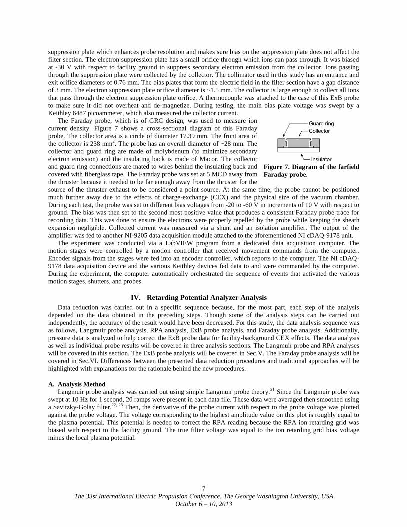
The Faraday probe, which is of GRC design, was used to measure ion
current density. Figure 7 shows a cross-sectional diagram of this Faraday
probe. The collector area is a circle of diameter 17.39 mm. The front area of
the collector is 238 mm2. The probe has an overall diameter of ~28 mm. The
collector and guard ring are made of molybdenum (to minimize secondary
electron emission) and the insulating back is made of Macor. The collector
and guard ring connections are mated to wires behind the insulating back and
covered with fiberglass tape. The Faraday probe was set at 5 MCD away from
the thruster because it needed to be far enough away from the thruster for the
source of the thruster exhaust to be considered a point source. At the same time, the probe cannot be positioned
much further away due to the effects of charge-exchange (CEX) and the physical size of the vacuum chamber.
During each test, the probe was set to different bias voltages from -20 to -60 V in increments of 10 V with respect to
ground. The bias was then set to the second most positive value that produces a consistent Faraday probe trace for
recording data. This was done to ensure the electrons were properly repelled by the probe while keeping the sheath
expansion negligible. Collected current was measured via a shunt and an isolation amplifier. The output of the
amplifier was fed to another NI-9205 data acquisition module attached to the aforementioned NI cDAQ-9178 unit.
The experiment was conducted via a LabVIEW program from a dedicated data acquisition computer. The
motion stages were controlled by a motion controller that received movement commands from the computer.
Encoder signals from the stages were fed into an encoder controller, which reports to the computer. The NI cDAQ-
9178 data acquisition device and the various Keithley devices fed data to and were commanded by the computer.
During the experiment, the computer automatically orchestrated the sequence of events that activated the various
motion stages, shutters, and probes.
IV. Retarding Potential Analyzer Analysis
Data reduction was carried out in a specific sequence because, for the most part, each step of the analysis
depended on the data obtained in the preceding steps. Though some of the analysis steps can be carried out
independently, the accuracy of the result would have been decreased. For this study, the data analysis sequence was
as follows, Langmuir probe analysis, RPA analysis, ExB probe analysis, and Faraday probe analysis. Additionally,
pressure data is analyzed to help correct the ExB probe data for facility-background CEX effects. The data analysis
as well as individual probe results will be covered in three analysis sections. The Langmuir probe and RPA analyses
will be covered in this section. The ExB probe analysis will be covered in Sec.V. The Faraday probe analysis will be
covered in Sec.VI. Differences between the presented data reduction procedures and traditional approaches will be
highlighted with explanations for the rationale behind the new procedures.
A. Analysis Method
Langmuir probe analysis was carried out using simple Langmuir probe theory.21
Since the Langmuir probe was
swept at 10 Hz for 1 second, 20 ramps were present in each data file. These data were averaged then smoothed using
a Savitzky-Golay filter.22, 23
Then, the derivative of the probe current with respect to the probe voltage was plotted
against the probe voltage. The voltage corresponding to the highest amplitude value on this plot is roughly equal to
the plasma potential. This potential is needed to correct the RPA reading because the RPA ion retarding grid was
biased with respect to the facility ground. The true filter voltage was equal to the ion retarding grid bias voltage
minus the local plasma potential.
Figure 7. Diagram of the farfield
Faraday probe.

The 33st International Electric Propulsion Conference, The George Washington University, USA
October 6 – 10, 2013
8
RPA analysis was carried out by first smoothing the
RPA trace then taking the negative of the derivative of the
collector current with respect to the bias voltage on the ion
retarding grid. The result, plotted against the bias voltage, is
proportional to the ion energy per charge distribution
function.24
Traditionally, the most probable voltage is taken
as the average ion energy per charge. The most probable
voltage is defined as the voltage where the amplitude of the
plot maximizes. However, due to a combination of noise
and broad ion distribution, the data can sometimes contain
small bumps on top of the main population that skewed the
location of the most probable voltage. To deal with this
issue, the average ion energy per charge was calculated via
ensemble-averaging using only the part of the trace where
the amplitude exceeded half of the maximum amplitude.
This averaging approach will be referred to as the
threshold-based averaging approach with a 50% threshold.
For clean traces, this approach yield values that are at most
3-4 V different from the most probable voltage. For noisy
traces, this approach yield values that are insensitive to
noise spikes. Figure 8 shows plots from applying the threshold-based averaging approach to a slightly noisy RPA
trace. The black dashed vertical line indicates the location of the most probable voltage, the red solid vertical line
indicates the result of using the threshold-based averaging approach with the 50% threshold, and the red dashed
horizontal line indicates the 50% of maximum threshold.
Note that in theory the most accurate result is obtained by ensemble-averaging the entire RPA trace. However,
doing so often produces unphysical results because the ion energy per charge distribution as measured by the RPA is
typically much broader than the real distribution due to the wide acceptance angle of the RPA. This is also the
reason the traditional approach relies on the most probable voltage. Using the 50% threshold-based ensemble-
averaging approach essentially strikes a balance between excluding broadened data and maintaining some degree of
noise insensitivity.
A full uncertainty analysis will not be carried out for every element of this study. Only uncertainties associated
with novel parts of the study and uncertainties that are dominant will be analyzed. The uncertainty in the voltage
utilization as calculated from Eq. (3) is ~1%. This uncertainty is a combination of the uncertainty in the RPA
analysis method and the Langmuir probe analysis method used to correct the RPA measurement.
B. RPA and Langmuir Probe Results and Comparisons
Figure 9 shows example RPA traces from the same
reference point (400 V, 20 kW) for the 300M and 300MS.
This figure illustrates a common trend seen in the RPA data;
the distributions appear to be wider with a longer and fatter
energy tail for the 300MS than for the 300M. Note that the
distributions derived from the RPA are broadened by the
somewhat poor resolution of the probe, which has a tendency
to wash out differences between the thrusters. Thus, the real
differences between the energy distribution functions of the
300M and 300MS are expected to be greater than indicated
by the RPA and are difficult to quantify.
Table 1 summarizes the results of the RPA and Langmuir
probe analyses for all three thruster versions across the eight
reference points. At the bottom of the table, the average and
standard deviation of the voltage utilization efficiency across
the eight reference points are shown. The averages show,
more clearly, the differences in values between the three
thruster versions. The standard deviations give indications of the spread in values across the eight reference points.
By comparing the standard deviations, one can get a sense of whether the spread changes with thruster versions,
which may indicate a change in thruster physics. A change in spread can also indicate a change in the noise
Figure 8. Sample RPA analysis plots.
Figure 9. Comparison of ion energy-per-charge
distributions for the 300M and 300MS at 400 V,
20 kW.

The 33st International Electric Propulsion Conference, The George Washington University, USA
October 6 – 10, 2013
9
environment of the probe. Thus, care should be taken when interpreting the standard deviation, especially if the
amplitude of the difference is lower than the uncertainty of the probe data. From Table 1, one can see that the three
thruster versions behave largely the same in terms of voltage utilization. Both versions of the 300MS perform
slightly better than the 300M.
Note that some values of energy per charge for the 300MS and 300MS-2 are very close to the discharge voltage
and seem physically impossible at first glance given that some ~10 volts of the discharge voltage must be used to
extract electrons from the cathode. However, one should keep in mind that the total possible voltage drop from
anode to cathode actually includes the drop across the anode sheath. Thus the true maximum total voltage drop is
slightly higher than the discharge voltage. While accounting for the anode sheath voltage is interesting, this quantity
is not easy to measure. The total discharge power is still easiest to calculate by using the discharge voltage with the
discharge current so the efficiency model presented here uses the discharge voltage to calculate voltage utilization.
V. ExB Probe Analysis
A. Analysis Method
The ExB probe is used as a velocity filter for charged species spectrometry. Since different charged species are
accelerated to different velocities by going through roughly the same potential drop, they will show up as different
peaks when interrogated by the ExB probe. For a scenario where the ExB probe velocity resolution is at least several
times smaller than the width of the ion velocity distribution function (VDF), the preferred method for analyzing ExB
probe data is via integration. In the past, most integration schemes involved fitting some general distribution
equation form to the ExB probe trace and calculating either by geometry or by numerical integration the area under
the curve.12, 25, 26
This is done because the ion distributions from different charged species tend to overlap in the
regions between peaks, making a direct integration of only one species at a time impossible without some kind of
assumption on the form of the distribution. The domain of the curve-fit for each species usually needs to be bounded
such that only the current signal generated by one species is being fitted at a time.
In the process of carrying out the present study, the area under the curve was discovered to not be exactly
proportional to the current associated with each species. A new set of integration formulas were derived from
scratch for the purpose of analyzing ExB probe data. The results of the new derivation closely matches the
derivation by Kim27
, though Kim did not publish the species fraction formulas and did not try to calculate the
current fraction (that was not his objective). As such, the new derivation continues where Kim’s work left off.
Note that Kim’s work27
is the first published instance where the ExB probe was used to study a Hall thruster and
strongly influenced all subsequent work in this area including all other cited work on ExB probe studies.
Full derivation of the new integration formulas for analyzing ExB probe data is presented in Appendix A.
Additional mathematical comparisons between the traditional and new integration formulas are shown in Appendix
B. The ExB probe data presented in this paper are analyzed using the following steps.
In the first step, one begins by selecting a form for the VDF. A number of different VDF forms were tried
including the triangle, similar to what was proposed by Beal,25
the Gaussian, first proposed by Linnell,26
and the
Table 1. Summary of voltage utilization analysis.
Plasma
potential, V
Energy per
charge, V
Voltage utilization
efficiency
Disch.
voltage,
V
Disch.
power,
kW 30
0M
30
0M
S
30
0M
S-2
30
0M
30
0M
S
30
0M
S-2
30
0M
30
0M
S
30
0M
S-2
300 10 6.3 7.6 7.2 278 285 288 0.926 0.947 0.957 300 15 6.3 6.4 7.0 281 281 291 0.934 0.935 0.969 400 10 6.9 7.7 8.0 377 389 395 0.942 0.972 0.984 400 15 7.4 7.7 8.1 377 385 391 0.940 0.961 0.978 400 20 6.9 7.2 7.2 378 390 396 0.943 0.974 0.987 500 10 6.9 8.1 7.6 481 473 484 0.962 0.946 0.968 500 15 7.9 8.1 8.1 472 491 491 0.942 0.980 0.982 500 20 7.9 8.1 7.8 480 491 496 0.959 0.981 0.992
Average: 0.944 0.962 0.977 Std. dev.: 0.012 0.017 0.012
The 33st International Electric Propulsion Conference, The George Washington University, USA
October 6 – 10, 2013
10
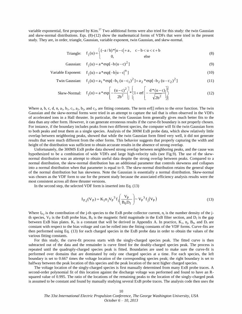
variable exponential, first proposed by Kim.27
Two additional forms were also tried for this study: the twin Gaussian
and skew-normal distributions. Eqs. (8)-(12) show the mathematical forms of VDFs that were tried in the present
study. They are, in order, triangle, Gaussian, variable exponent, twin Gaussian, and skew-normal.
Triangle:
else,0
bcubc,acu*)b/a()u(f j (8)
Gaussian: ])cu(bexp[*a)u(f 2j
(9)
Variable Exponent: ]cubexp[*a)u(fn
j
(10)
Twin Gaussian: ])cu(bexp[*a])cu(bexp[*a)u(f 2222
2111j
(11)
Skew-Normal:
22
2
j
b2
)cu(*derf1*
b2
)cu(exp*a)u(f (12)
Where a, b, c, d, n, a1, b1, c1, a2, b2, and c2, are fitting constants. The term erf[] refers to the error function. The twin
Gaussian and the skew-normal forms were tried in an attempt to capture the tail that is often observed in the VDFs
of accelerated ions in a Hall thruster. In particular, the twin Gaussian form generally gives much better fits to the
data than any other form. However, it can generate erroneous results if the curve-fit boundary is not properly chosen.
For instance, if the boundary includes peaks from two different species, the computer will fit the twin Gaussian form
to both peaks and treat them as a single species. Analysis of the 300M ExB probe data, which show relatively little
overlap between neighboring peaks, showed that while the twin Gaussian form fitted very well, it did not generate
results that were much different from the other forms. This behavior suggests that properly capturing the width and
height of the distribution was sufficient to obtain accurate results in the absence of strong overlap.
Unfortunately, the 300MS ExB probe data showed strong overlap between neighboring peaks, and the cause was
hypothesized to be a combination of wide VDFs and large high-velocity tails (see Fig.9). The use of the skew-
normal distribution was an attempt to obtain useful data despite the strong overlap between peaks. Compared to a
normal distribution, the skew-normal distribution has an additional parameter that controls skewness and collapses
into a normal distribution when that parameter is equal to 0. The skew-normal distribution retains the general shape
of the normal distribution but has skewness. Note the Gaussian is essentially a normal distribution. Skew-normal
was chosen as the VDF form to use for the present study because the associated efficiency analysis results were the
most consistent across all three thruster versions.
In the second step, the selected VDF form is inserted into Eq. (13)
Pj
3P
f0
Pj
3Pj1PjP, VfV~
DB
VfVnK)V(I
(13)
Where IP,j is the contribution of the j-th species to the ExB probe collector current, nj is the number density of the j-
th species, VP is the ExB probe bias, B0 is the magnetic field magnitude in the ExB filter section, and Df is the gap
between ExB bias plates. K1 is a constant that will be derived in Appendix A. In practice, K1, nj, B0, and Df are
constant with respect to the bias voltage and can be rolled into the fitting constants of the VDF forms. Curve-fits are
then performed using Eq. (13) for each charged species in the ExB probe data in order to obtain the values of the
various fitting constants.
For this study, the curve-fit process starts with the singly-charged species peak. The fitted curve is then
subtracted out of the data and the remainder is curve fitted for the doubly-charged species peak. The process is
repeated until the quadruply-charged species peak is fitted. Boundaries are used to make sure the curve-fit is
performed over domains that are dominated by only one charged species at a time. For each species, the left
boundary is set to 0.667 times the voltage location of the corresponding species peak; the right boundary is set to
halfway between the peak location of this species and the peak location of the next higher charged species.
The voltage location of the singly-charged species is first manually determined from many ExB probe traces. A
second-order polynomial fit of this location against the discharge voltage was performed and found to have an R-
squared value of 0.995. The ratio of the locations of the remaining peaks to the location of the singly-charged peak
is assumed to be constant and found by manually studying several ExB probe traces. The analysis code then uses the

The 33st International Electric Propulsion Conference, The George Washington University, USA
October 6 – 10, 2013
11
discharge voltage, the second-order polynomial fit, and the peak location ratios to predict the location where each
charged species should be located. For ExB probe traces with distinguishable peaks, visual inspection of the curve-
fit process shows the code accurately predicts the peak locations.
Figure 10 shows a set of analysis plots generated by the program that performs the ExB probe analysis. The
thruster is the 300M and the operating condition is 500 V, 20 kW. For convenience, the paper will refer to the six
subplots in order from left to right, top to bottom as (a) to (f). Subplot (a) shows the raw ExB probe data as black
data points with red dashed vertical lines showing the location of the first four peaks. Subplots (b), (c), (e), and (f)
show the four sub-steps in the curve-fitting process. The program fits the appropriate equation to the 1st peak,
subtracts the fitted data, then fits the 2nd
peak, and so on. The data prior to the fit at each curve-fit sub-step is shown
as black dots, the red solid line shows the curve-fit, the magenta dashed vertical lines show the curve-fit boundaries,
and the blue dashed line shows the leftover result after subtraction. Subplot (d) shows the raw data in black dots with
a red solid line that represents the sum of all four curve-fit sub-steps super-imposed on top. Figure 11 shows the
same for the 300MS.
In the third step, the IP,j of all the species are substituted into Eqs. (14) and (15) to calculate the species and
current fractions, respectively,
Figure 10. ExB probe analysis plots for the 300M operating at 500 V, 20 kW.
Figure 11. ExB probe analysis plots for the 300MS operating at 500 V, 20 kW.

The 33st International Electric Propulsion Conference, The George Washington University, USA
October 6 – 10, 2013
12
k
P0 3
P
Pk,P
P0 3
P
Pj,P
k
k
jj
dVV
)V(I
dVV
)V(I
n
n (14)
k
P0 2
P
Pk,Pk
P0 2
P
Pj,Pj
k
k
jj
dVV
)V(IZ
dVV
)V(IZ
I
I (15)
Where Ij is the current contributed by the j-th species at the entrance of the ExB probe collimator. Since the entrance
orifice area is a constant across all Ij’s, Ij and Ik can be replaced with the corresponding current densities. Note that Ij
is not the same as IP,j, which is current at the collector of the ExB probe. In this study, Xe4+
was not accounted for in
the current and species fraction calculation because those typically comprise less than 0.5% of the beam current.
In the fourth step, CEX interactions between beam ions and facility background neutrals were accounted for.
CEX depletes lower-charge-state species more than higher-charge-state species, causing the ExB probe to read more
higher-charge-state species than when in the vacuum of space. This effect is especially prominent for high-power
thruster tests. The CEX model used to correct the ExB probe data is described in Shastry’s work12
. The model
describes the effect of CEX as a set of attenuation factors that diminishes the detected current at the ExB collector.
Eqs. (16)-(18) show the equations used to calculate the attenuation factors.12
)Vlog(6.133.87),znexp()(J/J 1110Xe0
(16)
)V2log(9.87.45),znexp()(J/J 2220Xe0 2 (17)
)V3log(0.39.16),znexp()(J/J 3330Xe0 3
(18)
Where J is the recorded current density at distance z away from the thruster exit plane, J0 is the current density that
would have been recorded at the thruster exit plane, and n0 is the average background neutral density. The numerical
formulas for the CEX cross-sections, σ1, σ2, and σ3, are given in units of Å2 (10
-20 m
2). The ion energy per charge,
V1, V2, and V3 for Xe+, Xe
2+, and Xe
3+, respectively, are assumed to be equal to the average ion energy per charge as
measured by the RPA. The value of n0 is calculated by converting the average of the pressure measurement from
four ion gauges. Two of these gauges were located on the chamber wall at the same axial position as the farfield
probe tower, one of the gauges was next to the thrust stand, and the last of the gauges was on the chamber wall at an
axial location close to the thruster. Note that one can assume the ion energy per charge is equal to the discharge
voltage for the purpose of these calculations. Doing so removes the dependence of the ExB probe analysis on the
RPA, though with a small increase in uncertainty. See Shastry’s work for an estimate of this uncertainty.12
The uncertainty in the charge utilization as calculated from Eq. (7) is no more than 0.5%. This value is small
because the charge utilization is very insensitive to the values of the current fractions. For the 300M, the charge
utilization varied from 0.975 to 0.984. For the 300MS, the charge utilization varied from 0.965 to 0.973.
ExB probe data is also used to calculate the m term in the mass utilization. Total uncertainty of the mass
utilization will be discussed in Sec.VI; this paragraph will focus on the uncertainty in m. Based on the equations
derived in the appendix, the average velocity resolution of the ExB probe was 2.7%. This value is higher for ions
with higher energy per charge and is no more than 4.0% for the detectable ion populations with the highest energy
per charge. This resolution is sufficiently fine so that the aforementioned ExB probe analysis method is applicable.
The ExB probe resolution primarily affected broadening of the measured VDF and has minimal effect on the current
fractions. For the 300M, the uncertainty in the current fraction is expected to be dominated by the uncertainty in the
average background neutral density measured by the ion gauges. For the 300MS, additional uncertainty is
introduced by the strong overlap between charged species peaks. This added uncertainty arises from not being
certain about whether the analysis program really only captured contributions from one charged species at a time.
For now we will focus on the uncertainty in the ion gauge measurements. The ion gauges are nominally 6%
accurate. However, they only measured the neutral density in their immediate vicinity. Factors like conductance
losses and un-compensated temperature effects on the electronics are expected to raise the uncertainty of the neutral
The 33st International Electric Propulsion Conference, The George Washington University, USA
October 6 – 10, 2013
13
density measurement to ~15%. Substituting in a ±15% neutral
density uncertainty into the CEX correction formula yielded
average uncertainties of ±0.034, ±0.024, and ±0.011 for the
Xe+, Xe
2+, and Xe
3+ current fractions, respectively. The
corresponding average uncertainty for m is ~2%. Since
much is still not known about the strong overlap between
peaks found in the ExB probe traces of the 300MS, the
uncertainty in m for the 300MS will be tentatively set to
twice that of the 300M. Thus, the uncertainty in m is 2% for
the 300M and 4% for the 300MS.
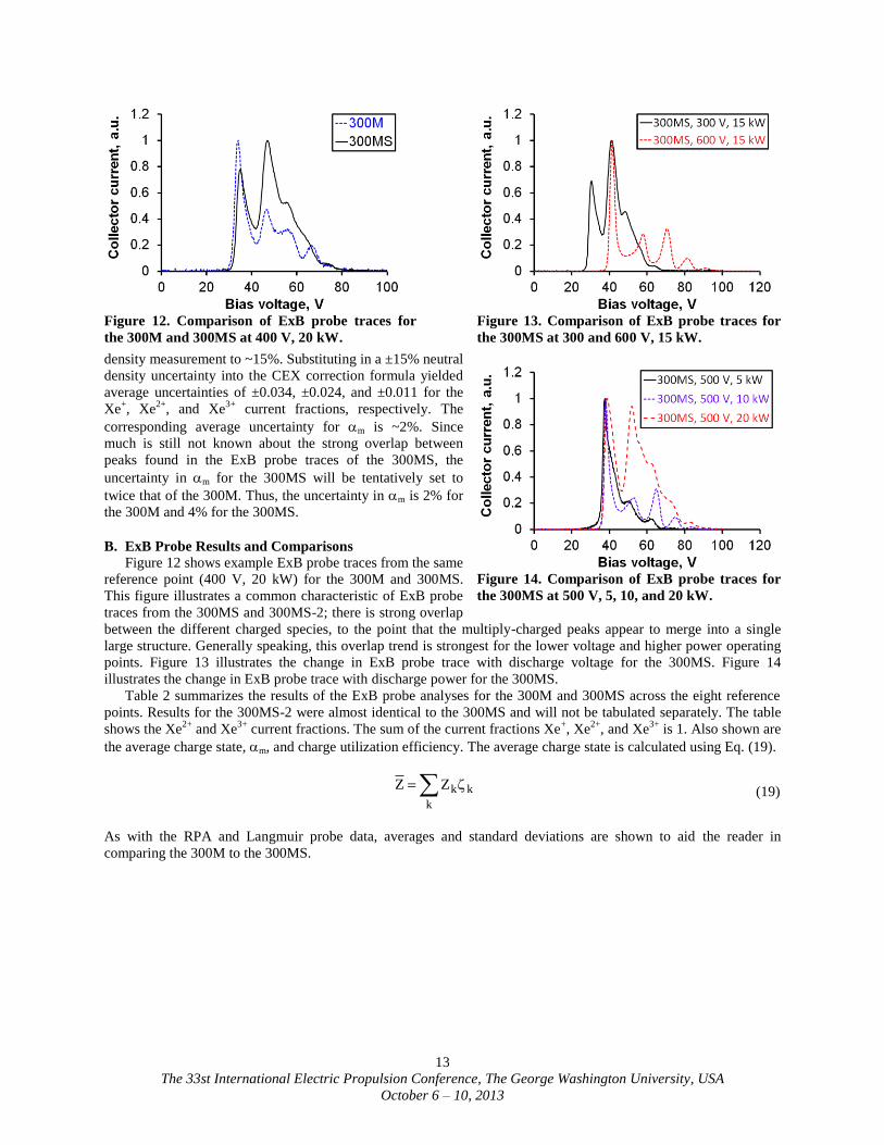
B. ExB Probe Results and Comparisons
Figure 12 shows example ExB probe traces from the same
reference point (400 V, 20 kW) for the 300M and 300MS.
This figure illustrates a common characteristic of ExB probe
traces from the 300MS and 300MS-2; there is strong overlap
between the different charged species, to the point that the multiply-charged peaks appear to merge into a single
large structure. Generally speaking, this overlap trend is strongest for the lower voltage and higher power operating
points. Figure 13 illustrates the change in ExB probe trace with discharge voltage for the 300MS. Figure 14
illustrates the change in ExB probe trace with discharge power for the 300MS.
Table 2 summarizes the results of the ExB probe analyses for the 300M and 300MS across the eight reference
points. Results for the 300MS-2 were almost identical to the 300MS and will not be tabulated separately. The table
shows the Xe2+
and Xe3+
current fractions. The sum of the current fractions Xe+, Xe
2+, and Xe
3+ is 1. Also shown are
the average charge state, m, and charge utilization efficiency. The average charge state is calculated using Eq. (19).
k
kkZZ (19)
As with the RPA and Langmuir probe data, averages and standard deviations are shown to aid the reader in
comparing the 300M to the 300MS.
Figure 12. Comparison of ExB probe traces for
the 300M and 300MS at 400 V, 20 kW.
Figure 13. Comparison of ExB probe traces for
the 300MS at 300 and 600 V, 15 kW.
Figure 14. Comparison of ExB probe traces for
the 300MS at 500 V, 5, 10, and 20 kW.

The 33st International Electric Propulsion Conference, The George Washington University, USA
October 6 – 10, 2013
14
Table 2 shows that the 300MS is producing ~70% more
multiply charged particles than the 300M on the average.
This rise in multiply charged species has a much more
prominent effect on the value of m than on the charge
utilization efficiency. The low magnitude of the standard
deviation shows that the difference in m between the 300M
and 300MS is not a statistical fluke. While Table 2 shows the
average trends across thrusters, detailed trends are difficult to
visualize from Table 2. Figure 15 shows a plot of the average
charge state as a function of the discharge current. Since the
channel cross section (upstream of the chamfers) was kept the
same between the 300M and 300MS, the discharge current is
proportional to the current density. Note that this figure is
augmented with data from operating points beyond the eight
reference points. A rather interesting trend can be seen in this
figure. Whereas the average charged state of the 300M remained comparatively constant (to within ±0.03), the same
of the 300MS increase quite noticeably with discharge current (and current density). This rise is most rapid at lower
discharge current and tapers off at higher discharge current. The change in multiply charged species content is one
of the biggest differences between the 300M and 300MS.
VI. Faraday Probe Analysis
A. Analysis Method
Faraday probe data are used to calculate the plume divergence angle and the total ion beam current. The cosine
of the momentum-weighted plume divergence angle is defined as the average axial velocity of the particles divided
by the average total velocity of the particles. However, momentum-weighted divergence angle is difficult to
measure. The typical approach is to measure the charge-weighted divergence angle, which is approximately equal to
the momentum-weighted divergence angle if the current fraction is roughly constant across the interrogated domain.
For a polarly-swept probe, Eq. (20) can be used to calculate the charge-weighted divergence angle.
2/
0
2FP
2/
0
2FP
dsin)j(R2
dsinθcos)j(R2
δcos (20)
Table 2. Summary of charge utilization and αm analyses.
Current
fraction,
Xe2+
Current
fraction,
Xe3+
Average
charge state m
Charge
utilization
efficiency
Disch.
voltage,
V
Disch.
power,
kW 30
0M
30
0M
S
30
0M
30
0M
S
30
0M
30
0M
S
30
0M
30
0M
S
30
0M
30
0M
S
300 10 0.18 0.34 0.04 0.05 1.097 1.195 0.884 0.800 0.980 0.971 300 15 0.24 0.31 0.03 0.08 1.125 1.201 0.858 0.793 0.977 0.968 400 10 0.21 0.33 0.05 0.03 1.122 1.181 0.861 0.811 0.976 0.973 400 15 0.19 0.32 0.06 0.07 1.116 1.205 0.865 0.789 0.976 0.968 400 20 0.18 0.32 0.05 0.09 1.102 1.214 0.878 0.781 0.978 0.967 500 10 0.22 0.27 0.06 0.12 1.134 1.207 0.851 0.786 0.975 0.965 500 15 0.19 0.31 0.05 0.06 1.115 1.187 0.867 0.805 0.977 0.970 500 20 0.20 0.33 0.06 0.09 1.123 1.222 0.858 0.776 0.975 0.967
Average: 0.20 0.32 0.05 0.07 1.117 1.201 0.865 0.793 0.977 0.969 Std. dev.: 0.011 0.012 0.002 0.003
Figure 15. Average charge state as a function of
discharge current for the 300M and 300MS.

The 33st International Electric Propulsion Conference, The George Washington University, USA
October 6 – 10, 2013
15
Where δ is the charged-weighted divergence angle, θ is the
polar angle and is equal to 0° for particles traveling parallel
to the firing axis, and j(θ) is the ion current density as a
function of the polar angle. RFP is the distance from the
Faraday probe collector to the thruster center at the exit
plane and is constant for a polarly-swept probe. Note the
denominator is equal to the total ion beam current.
For a nude Faraday probe with a guard ring like the one
used in this study, the effective collector area is not exactly
equal to the collector frontal surface area. Current that
enters the gap between the collector and the guard ring can
be collected by the side surfaces of the collector.28
According to work by Brown, the current entering the gap is
collected by the collector and the guard ring in ratio
proportional to the ratio of exposed gap area.28
For the
probe design used in the present study, the area inside the gap is
dominated by area connected to the guard ring (See Fig. 7).
However there is enough area connected to the collector that
some level of correction is needed. Note that only the part of the
gap with direct exposure to the incoming ion beam is used in
the gap area calculation. Using the approach recommended by
Brown, the effective collection area is ~4% greater than the
collector frontal area. The effective collection area is used for
all Faraday probe analysis.
Much like in ExB probe data analysis, CEX is a factor in Faraday probe data analysis. However, whereas CEX is
an attenuating factor for ExB probe data, it is a re-distributing factor for Faraday probe data. This is because CEX
ions have a different trajectory than the ion it is born from and will tend to show up in the wings of a Faraday probe
trace. The region considered the “wings” of a Faraday probe trace can be seen in Fig. 16 as the region outside of the
two outermost dashed vertical lines. An ExB probe does not see CEX ions because of a combination of small
acceptance angle and a tendency to de-emphasize low speed ions. The ExB filter resolution has a dependence on the
square of the particle speed and CEX ions have only a small fraction of the speed of beam ions. The best way to
correct for the re-distributing behavior of CEX on Faraday probe traces is to take data at multiple distances and
facility background pressures.28
This could not be carried out for the present study due to space constraints. Instead,
an extrapolated-wing approach was used to remove the parts of the trace that are believed to be dominated by re-
distributed CEX ions. The extrapolated-wing approach begins by plotting the ion current density on a semi-log
scale. Exponential curve-fits are then performed on the data from a polar angle of 10° to 25°. The curve-fit result is
then extrapolated to 90°. Note an exponential function of the polar angle shows up as straight lines on the semi-log
plot. Figure 16 shows a graphical representation of the extrapolated-wing method. The black solid line is the raw
data. The dashed vertical line in the middle is the center of the trace (θ is not quite equal to 0° here due to a minor
mis-alignment in the physical setup). The left two and right two dashed vertical lines indicate the boundary for the
data used to perform the curve-fit on the respective side. The light green solid lines represent the curve-fit results.
In past studies, low secondary electron emission (SEE) yield materials like molybdenum and tungsten have been
used for the collector.29-31
Secondary electrons born on a negatively biased probe will accelerate away from the
probe. This effect adds extra current to the probe measurement that is indistinguishable from the collected ion
current. By selecting a low SEE yield material, researchers had believed that the effect of SEE is negligible and can
be ignored. While singly-charged xenon-induced SEE yield for molybdenum and tungsten are indeed negligible
(0.013 to 0.022), the doubly-charged xenon-induced SEE yield are roughly 10 times higher than the singly-charged
yield, and the triply-charged SEE yield are roughly 35 times higher than the singly-charged yield.32-34
Furthermore,
Hagstrum discovered that metastable singly-charged xenon induces roughly the same SEE yield as doubly-charged
xenon.35
Thus, as long as the plume of the thruster is composed of mostly ground-state singly-charged xenon ions,
the assumption of negligible SEE effect holds.
During the present testing, the assumption of negligible SEE effect was discovered to not hold. The material
used for the present study is molybdenum, which is considered a low SEE yield material. The reason SEE effects are
not negligible is because high-power Hall thrusters appear to produce 20-40% doubly- and triply-charged ions by
current fraction. Combined with the high SEE yield associated with bombardment by higher charge ions, the effect
of SEE can be non-negligible. To correct for SEE effects on the Faraday probe measurement, we turn to data
Figure 16. Illustration of the extrapolated-wing
method for analyzing Faraday probe data.
Table 3. Summary of SEE data for xenon ion
bombardment of molybdenum.32, 33
Bombarding
particle
SEE yield of
molybdenum
Xe+ 0.022
Xe2+
0.20
Xe3+
0.70
The 33st International Electric Propulsion Conference, The George Washington University, USA
October 6 – 10, 2013
16
published by Hagstrum. Table 3 summarizes the SEE yield values used in the data analysis of the present study. The
singly-charged and doubly-charged xenon-induced yields are averages of the SEE yield data for ion energies in the
range of 200 to 800 eV in Hagstrum’s 1956 work on molybdenum.33
For both of these parameters, the value
measured by Hagstrum varied by no more than 10% of the listed average. A published value for the triply-charged
xenon-induced yield of molybdenum could not be found. The value in Table 3 is a projected value based on the
similarity in yield between tungsten and molybdenum. The ratio of triply-charged induced yield to doubly-charged
induced yield for tungsten is 3.5, so the yield for molybdenum is projected to be 3.5 * 0.2, or 0.7.32
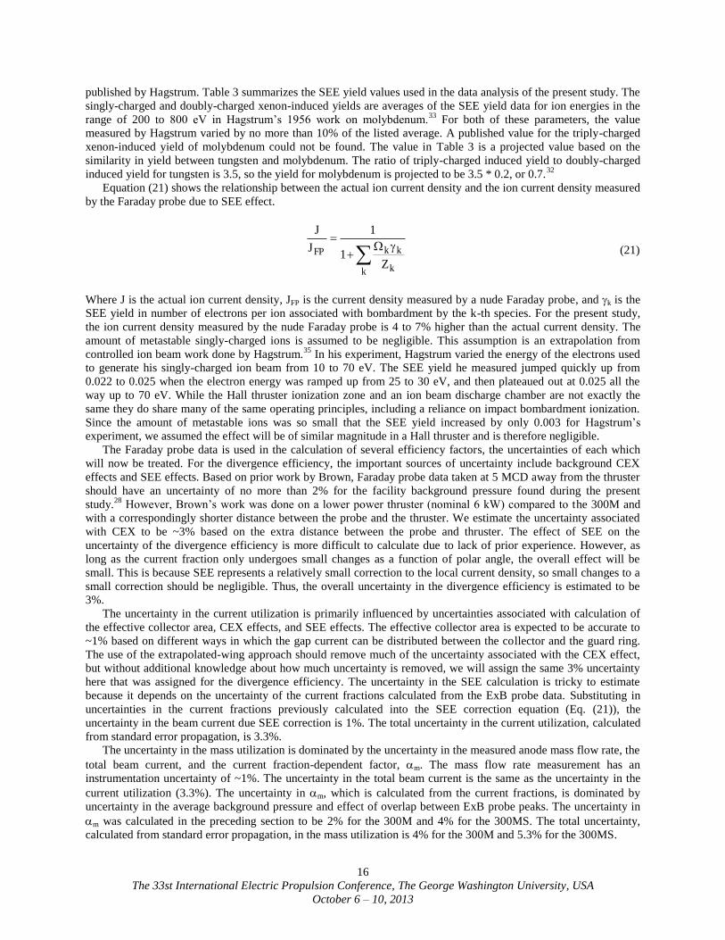
Equation (21) shows the relationship between the actual ion current density and the ion current density measured
by the Faraday probe due to SEE effect.
k k
kkFP
Z1
1
J
J
(21)
Where J is the actual ion current density, JFP is the current density measured by a nude Faraday probe, and k is the
SEE yield in number of electrons per ion associated with bombardment by the k-th species. For the present study,
the ion current density measured by the nude Faraday probe is 4 to 7% higher than the actual current density. The
amount of metastable singly-charged ions is assumed to be negligible. This assumption is an extrapolation from
controlled ion beam work done by Hagstrum.35
In his experiment, Hagstrum varied the energy of the electrons used
to generate his singly-charged ion beam from 10 to 70 eV. The SEE yield he measured jumped quickly up from
0.022 to 0.025 when the electron energy was ramped up from 25 to 30 eV, and then plateaued out at 0.025 all the
way up to 70 eV. While the Hall thruster ionization zone and an ion beam discharge chamber are not exactly the
same they do share many of the same operating principles, including a reliance on impact bombardment ionization.
Since the amount of metastable ions was so small that the SEE yield increased by only 0.003 for Hagstrum’s
experiment, we assumed the effect will be of similar magnitude in a Hall thruster and is therefore negligible.
The Faraday probe data is used in the calculation of several efficiency factors, the uncertainties of each which
will now be treated. For the divergence efficiency, the important sources of uncertainty include background CEX
effects and SEE effects. Based on prior work by Brown, Faraday probe data taken at 5 MCD away from the thruster
should have an uncertainty of no more than 2% for the facility background pressure found during the present
study.28
However, Brown’s work was done on a lower power thruster (nominal 6 kW) compared to the 300M and
with a correspondingly shorter distance between the probe and the thruster. We estimate the uncertainty associated
with CEX to be ~3% based on the extra distance between the probe and thruster. The effect of SEE on the
uncertainty of the divergence efficiency is more difficult to calculate due to lack of prior experience. However, as
long as the current fraction only undergoes small changes as a function of polar angle, the overall effect will be
small. This is because SEE represents a relatively small correction to the local current density, so small changes to a
small correction should be negligible. Thus, the overall uncertainty in the divergence efficiency is estimated to be
3%.
The uncertainty in the current utilization is primarily influenced by uncertainties associated with calculation of
the effective collector area, CEX effects, and SEE effects. The effective collector area is expected to be accurate to
~1% based on different ways in which the gap current can be distributed between the collector and the guard ring.
The use of the extrapolated-wing approach should remove much of the uncertainty associated with the CEX effect,
but without additional knowledge about how much uncertainty is removed, we will assign the same 3% uncertainty
here that was assigned for the divergence efficiency. The uncertainty in the SEE calculation is tricky to estimate
because it depends on the uncertainty of the current fractions calculated from the ExB probe data. Substituting in
uncertainties in the current fractions previously calculated into the SEE correction equation (Eq. (21)), the
uncertainty in the beam current due SEE correction is 1%. The total uncertainty in the current utilization, calculated
from standard error propagation, is 3.3%.
The uncertainty in the mass utilization is dominated by the uncertainty in the measured anode mass flow rate, the
total beam current, and the current fraction-dependent factor, m. The mass flow rate measurement has an
instrumentation uncertainty of ~1%. The uncertainty in the total beam current is the same as the uncertainty in the
current utilization (3.3%). The uncertainty in m, which is calculated from the current fractions, is dominated by
uncertainty in the average background pressure and effect of overlap between ExB probe peaks. The uncertainty in
m was calculated in the preceding section to be 2% for the 300M and 4% for the 300MS. The total uncertainty,
calculated from standard error propagation, in the mass utilization is 4% for the 300M and 5.3% for the 300MS.
The 33st International Electric Propulsion Conference, The George Washington University, USA
October 6 – 10, 2013
17
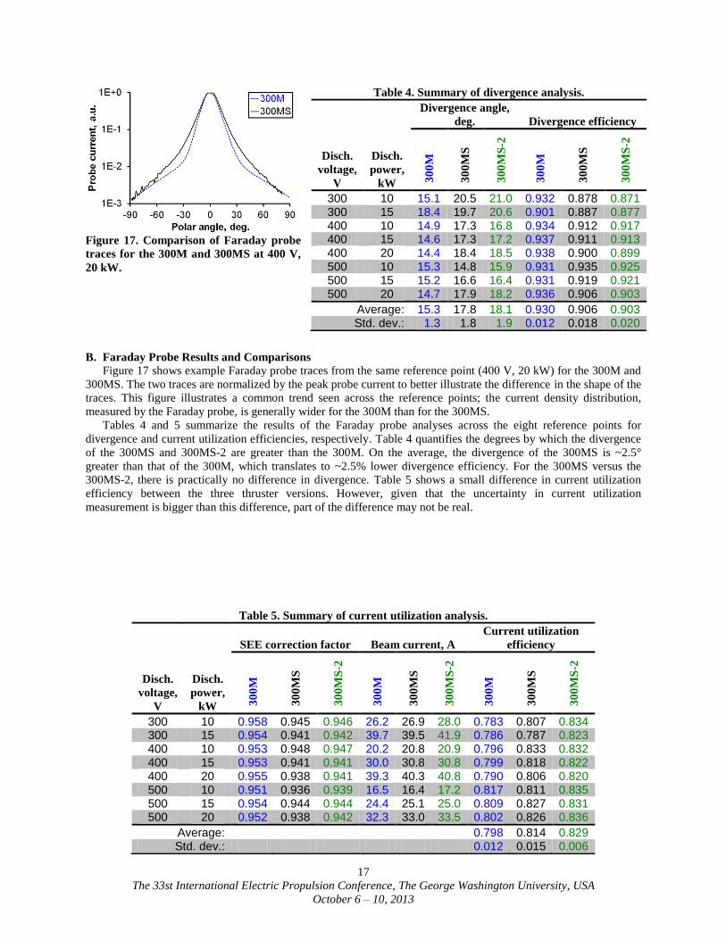
B. Faraday Probe Results and Comparisons
Figure 17 shows example Faraday probe traces from the same reference point (400 V, 20 kW) for the 300M and
300MS. The two traces are normalized by the peak probe current to better illustrate the difference in the shape of the
traces. This figure illustrates a common trend seen across the reference points; the current density distribution,
measured by the Faraday probe, is generally wider for the 300M than for the 300MS.
Tables 4 and 5 summarize the results of the Faraday probe analyses across the eight reference points for
divergence and current utilization efficiencies, respectively. Table 4 quantifies the degrees by which the divergence
of the 300MS and 300MS-2 are greater than the 300M. On the average, the divergence of the 300MS is ~2.5°
greater than that of the 300M, which translates to ~2.5% lower divergence efficiency. For the 300MS versus the
300MS-2, there is practically no difference in divergence. Table 5 shows a small difference in current utilization
efficiency between the three thruster versions. However, given that the uncertainty in current utilization
measurement is bigger than this difference, part of the difference may not be real.
Figure 17. Comparison of Faraday probe
traces for the 300M and 300MS at 400 V,
20 kW.
Table 4. Summary of divergence analysis.
Divergence angle,
deg. Divergence efficiency
Disch.
voltage,
V
Disch.
power,
kW 30
0M
30
0M
S
30
0M
S-2
30
0M
30
0M
S
30
0M
S-2
300 10 15.1 20.5 21.0 0.932 0.878 0.871 300 15 18.4 19.7 20.6 0.901 0.887 0.877 400 10 14.9 17.3 16.8 0.934 0.912 0.917 400 15 14.6 17.3 17.2 0.937 0.911 0.913 400 20 14.4 18.4 18.5 0.938 0.900 0.899 500 10 15.3 14.8 15.9 0.931 0.935 0.925 500 15 15.2 16.6 16.4 0.931 0.919 0.921 500 20 14.7 17.9 18.2 0.936 0.906 0.903
Average: 15.3 17.8 18.1 0.930 0.906 0.903 Std. dev.: 1.3 1.8 1.9 0.012 0.018 0.020
Table 5. Summary of current utilization analysis.
SEE correction factor Beam current, A
Current utilization
efficiency
Disch.
voltage,
V
Disch.
power,
kW 30
0M
30
0M
S
30
0M
S-2
30
0M
30
0M
S
30
0M
S-2
30
0M
30
0M
S
30
0M
S-2
300 10 0.958 0.945 0.946 26.2 26.9 28.0 0.783 0.807 0.834 300 15 0.954 0.941 0.942 39.7 39.5 41.9 0.786 0.787 0.823 400 10 0.953 0.948 0.947 20.2 20.8 20.9 0.796 0.833 0.832 400 15 0.953 0.941 0.941 30.0 30.8 30.8 0.799 0.818 0.822 400 20 0.955 0.938 0.941 39.3 40.3 40.8 0.790 0.806 0.820 500 10 0.951 0.936 0.939 16.5 16.4 17.2 0.817 0.811 0.835 500 15 0.954 0.944 0.944 24.4 25.1 25.0 0.809 0.827 0.831 500 20 0.952 0.938 0.942 32.3 33.0 33.5 0.802 0.826 0.836
Average: 0.798 0.814 0.829 Std. dev.: 0.012 0.015 0.006
The 33st International Electric Propulsion Conference, The George Washington University, USA
October 6 – 10, 2013
18
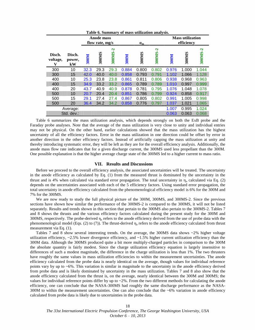
Table 6 summarizes the mass utilization analysis, which depends strongly on both the ExB probe and the
Faraday probe analyses. Note that the average of the mass utilization is very close to unity and individual entries
may not be physical. On the other hand, earlier calculations showed that the mass utilization has the highest
uncertainty of all the efficiency factors. Error in the mass utilization in one direction could be offset by error in
another direction in the other efficiency factors. Instead of artificially capping the mass utilization at unity and
thereby introducing systematic error, they will be left as they are for the overall efficiency analysis. Additionally, the
anode mass flow rate indicates that for a given discharge current, the 300MS used less propellant than the 300M.
One possible explanation is that the higher average charge state of the 300MS led to a higher current to mass ratio.
VII. Results and Discussions
Before we proceed to the overall efficiency analysis, the associated uncertainties will be treated. The uncertainty
in the anode efficiency as calculated by Eq. (1) from the measured thrust is dominated by the uncertainty in the
thrust and is 4% when calculated via standard error propagation. The total uncertainty in a calculated via Eq. (2)
depends on the uncertainties associated with each of the 5 efficiency factors. Using standard error propagation, the
total uncertainty in anode efficiency calculated from the phenomenological efficiency model is 6% for the 300M and
7% for the 300MS.
We are now ready to study the full physical picture of the 300M, 300MS, and 300MS-2. Since the previous
sections have shown how similar the performance of the 300MS-2 is compared to the 300MS, it will not be listed
separately. Results and trends shown in this section that pertain to the 300MS also pertain to the 300MS-2. Tables 7
and 8 shows the thrusts and the various efficiency factors calculated during the present study for the 300M and
300MS, respectively. The probe-derived ηa refers to the anode efficiency derived from the use of probe data with the
phenomenological model (Eqs. (2) to (7)). The thrust-derived ηa refers to the anode efficiency calculated from thrust
measurement via Eq. (1).
Tables 7 and 8 show several interesting trends. On the average, the 300MS data shows ~2% higher voltage
utilization efficiency, ~2.5% lower divergence efficiency, and ~1.5% higher current utilization efficiency than the
300M data. Although the 300MS produced quite a bit more multiply-charged particles in comparison to the 300M
the absolute quantity is fairly modest. Since the charge utilization efficiency equation is largely insensitive to
differences of such a modest magnitude, the difference in the charge utilization is less than 1%. The two thrusters
have roughly the same values in mass utilization efficiencies to within the measurement uncertainties. The anode
efficiency calculated from the probe data is nearly identical on the average, though values for individual reference
points vary by up to ~6%. This variation is similar in magnitude to the uncertainty in the anode efficiency derived
from probe data and is likely dominated by uncertainty in the mass utilization. Tables 7 and 8 also show that the
anode efficiency calculated from the thrust is, on the average, nearly identical between the 300M and 300MS; the
values for individual reference points differ by up to ~2%. From the two different methods for calculating the anode
efficiency, one can conclude that the NASA-300MS had roughly the same discharge performance as the NASA-
300M to within the measurement uncertainties. One can also conclude that the ~6% variation in anode efficiency
calculated from probe data is likely due to uncertainties in the probe data.
Table 6. Summary of mass utilization analysis.
Anode mass
flow rate, mg/s αm
Mass utilization
efficiency
Disch.
voltage,
V
Disch.
power,
kW 30
0M
30
0M
S
30
0M
S-2
30
0M
30
0M
S
30
0M
S-2
30
0M
30
0M
S
30
0M
S-2
300 10 32.3 29.3 29.3 0.884 0.800 0.802 0.976 1.000 1.044 300 15 42.0 40.0 40.0 0.858 0.793 0.791 1.102 1.066 1.128 400 10 25.3 23.8 23.8 0.861 0.811 0.806 0.938 0.968 0.963 400 15 34.9 33.2 33.2 0.865 0.789 0.789 1.010 0.997 0.999 400 20 43.7 40.9 40.9 0.878 0.781 0.795 1.076 1.048 1.078 500 10 20.7 20.4 20.4 0.851 0.786 0.799 0.924 0.858 0.917 500 15 29.1 27.4 27.4 0.867 0.805 0.802 0.991 1.005 0.998 500 20 36.4 34.2 34.2 0.858 0.776 0.797 1.037 1.021 1.065
Average: 1.007 0.995 1.024 Std. dev.: 0.063 0.063 0.068
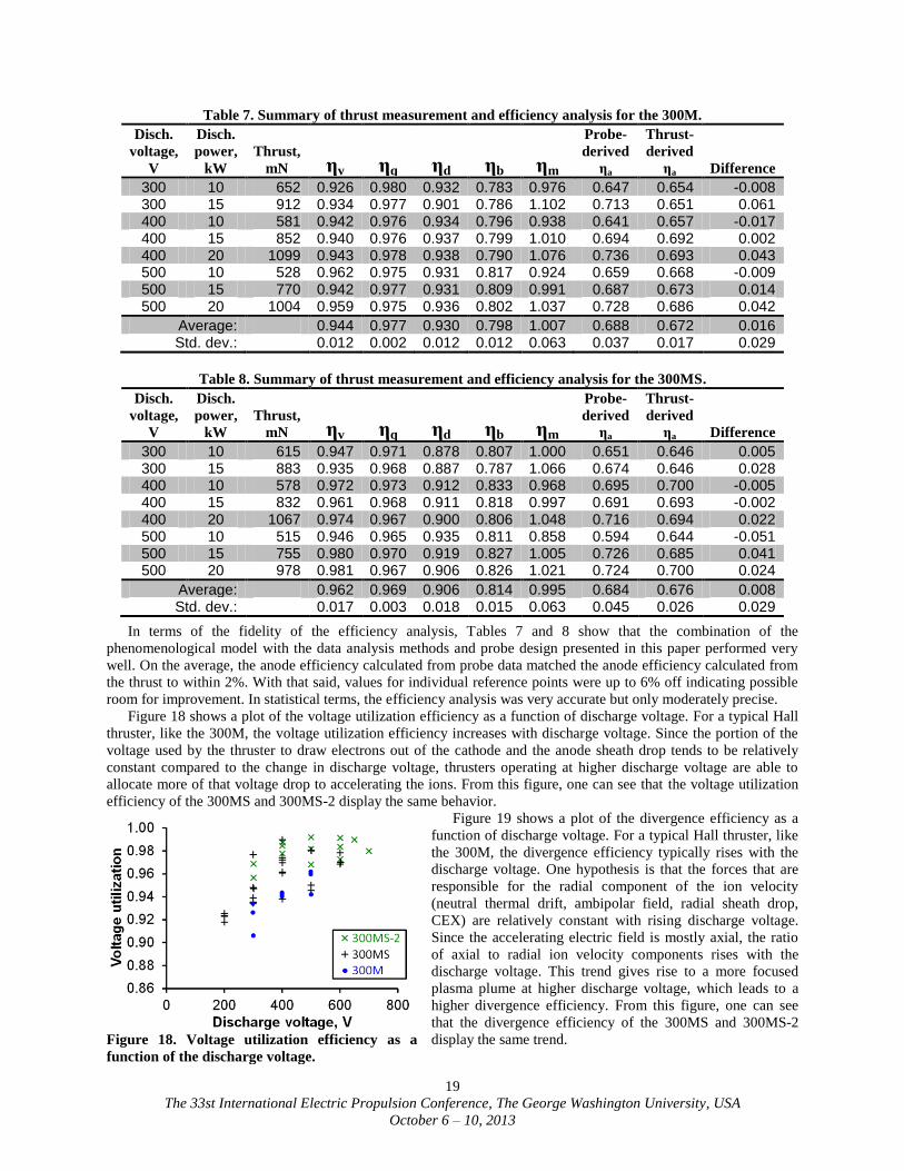
The 33st International Electric Propulsion Conference, The George Washington University, USA
October 6 – 10, 2013
19
In terms of the fidelity of the efficiency analysis, Tables 7 and 8 show that the combination of the
phenomenological model with the data analysis methods and probe design presented in this paper performed very
well. On the average, the anode efficiency calculated from probe data matched the anode efficiency calculated from
the thrust to within 2%. With that said, values for individual reference points were up to 6% off indicating possible
room for improvement. In statistical terms, the efficiency analysis was very accurate but only moderately precise.
Figure 18 shows a plot of the voltage utilization efficiency as a function of discharge voltage. For a typical Hall
thruster, like the 300M, the voltage utilization efficiency increases with discharge voltage. Since the portion of the
voltage used by the thruster to draw electrons out of the cathode and the anode sheath drop tends to be relatively
constant compared to the change in discharge voltage, thrusters operating at higher discharge voltage are able to
allocate more of that voltage drop to accelerating the ions. From this figure, one can see that the voltage utilization
efficiency of the 300MS and 300MS-2 display the same behavior.
Figure 19 shows a plot of the divergence efficiency as a
function of discharge voltage. For a typical Hall thruster, like
the 300M, the divergence efficiency typically rises with the
discharge voltage. One hypothesis is that the forces that are
responsible for the radial component of the ion velocity
(neutral thermal drift, ambipolar field, radial sheath drop,
CEX) are relatively constant with rising discharge voltage.
Since the accelerating electric field is mostly axial, the ratio
of axial to radial ion velocity components rises with the
discharge voltage. This trend gives rise to a more focused
plasma plume at higher discharge voltage, which leads to a
higher divergence efficiency. From this figure, one can see
that the divergence efficiency of the 300MS and 300MS-2
display the same trend.
Table 7. Summary of thrust measurement and efficiency analysis for the 300M.
Disch.
voltage,
V
Disch.
power,
kW
Thrust,
mN ηv ηq ηd ηb ηm
Probe-
derived
ηa
Thrust-
derived
ηa Difference
300 10 652 0.926 0.980 0.932 0.783 0.976 0.647 0.654 -0.008 300 15 912 0.934 0.977 0.901 0.786 1.102 0.713 0.651 0.061 400 10 581 0.942 0.976 0.934 0.796 0.938 0.641 0.657 -0.017 400 15 852 0.940 0.976 0.937 0.799 1.010 0.694 0.692 0.002 400 20 1099 0.943 0.978 0.938 0.790 1.076 0.736 0.693 0.043 500 10 528 0.962 0.975 0.931 0.817 0.924 0.659 0.668 -0.009 500 15 770 0.942 0.977 0.931 0.809 0.991 0.687 0.673 0.014 500 20 1004 0.959 0.975 0.936 0.802 1.037 0.728 0.686 0.042
Average: 0.944 0.977 0.930 0.798 1.007 0.688 0.672 0.016 Std. dev.: 0.012 0.002 0.012 0.012 0.063 0.037 0.017 0.029
Table 8. Summary of thrust measurement and efficiency analysis for the 300MS.
Disch.
voltage,
V
Disch.
power,
kW
Thrust,
mN ηv ηq ηd ηb ηm
Probe-
derived
ηa
Thrust-
derived
ηa Difference
300 10 615 0.947 0.971 0.878 0.807 1.000 0.651 0.646 0.005 300 15 883 0.935 0.968 0.887 0.787 1.066 0.674 0.646 0.028 400 10 578 0.972 0.973 0.912 0.833 0.968 0.695 0.700 -0.005 400 15 832 0.961 0.968 0.911 0.818 0.997 0.691 0.693 -0.002 400 20 1067 0.974 0.967 0.900 0.806 1.048 0.716 0.694 0.022 500 10 515 0.946 0.965 0.935 0.811 0.858 0.594 0.644 -0.051 500 15 755 0.980 0.970 0.919 0.827 1.005 0.726 0.685 0.041 500 20 978 0.981 0.967 0.906 0.826 1.021 0.724 0.700 0.024
Average: 0.962 0.969 0.906 0.814 0.995 0.684 0.676 0.008 Std. dev.: 0.017 0.003 0.018 0.015 0.063 0.045 0.026 0.029
Figure 18. Voltage utilization efficiency as a
function of the discharge voltage.

The 33st International Electric Propulsion Conference, The George Washington University, USA
October 6 – 10, 2013
20
The charge and current utilization efficiencies are largely constant and will not be plotted. Charge utilization is
largely constant due to the general insensitivity of the charge utilization equation to current fractions of the multiply-
charged species. The invariance of the current utilization with operating conditions have been seen in past work14, 16
The exact value of current utilization is related to electron mobility and is an ongoing area of research. Since the
value of the current utilization is largely constant for both the 300M and 300MS and are roughly equal, the same
transport mechanisms are likely to apply for both thrusters.
Figure 20 shows a plot of the mass utilization efficiency as a function of discharge current. For a typical Hall
thruster, like the 300M, the mass utilization efficiency typically rises with the discharge current. The reason is that
as the discharge current rise so does the current density and the plasma density. Since the ionization rate scales with
the electron density, denser plasma means higher ionization rate, which give rise to higher mass utilization. The
mass utilization efficiency of the 300MS and 300MS-2 display the same trends. Note that a value of mass utilization
above unity is unphysical. There are two potential sources of error that may explain some of the high mass
utilization values. As previously mentioned, the mass utilization draws heavily on both the ExB probe measurement
and the Faraday probe measurement. Inaccurate accounting of the multiply charged species such as poor handling of
the overlap region between charged peaks can give rise to incorrect values of αm and, by extension, the mass
utilization. For the Faraday probe data, the probe may be capturing more CEX than can be removed by the
extrapolated-wing method. If data from either (or both) probe(s) have a positive systematic error, the mass
utilization and the associated anode efficiency will be too high, which may explain why the probe-derived anode
efficiency is ~1% higher than the thrust-derived efficiency. With that said, the error being examined here is around
the same as or below the uncertainty of the measurements.
From the tables and figures in this section, one can conclude that the NASA-300MS likely operates on the same
ionization and acceleration physics as the NASA-300M. The implementation of magnetic shielding did not change
the fundamental laws that govern the basic operating principles of the 300M. The performance of the thruster
remained largely unchanged. We will now turn to the small differences that have been observed during the present
study and possible physical explanations.
Generally speaking, the plume of the 300MS contains more multiply charged species and has a higher
divergence than the plume of the 300M. One possible cause for the higher amount of multiply charged species is the
presence of higher temperature plasma associated with reduced wall moderation. The key idea behind magnetic
shielding is to maintain a layer of low-temperature, low-density plasma at high plasma potential near the channel
walls that extend all the way to the thruster exit.8 The anchor points of the magnetic lines of force that travel through
the bulk plasma are moved out of the channel and onto the front pole where plasma density is much lower (see
Fig. 21). As a result the wall area effectively “wetted” by the
plasma is reduced by orders of magnitude. In a typical Hall
thruster, like the 300M, where the lines of force that pass
through the bulk plasma terminates in the ceramic discharge
channel walls, electron temperature tends be moderated.
Ceramics, like boron nitride, have relatively high secondary
electron emission coefficients. When high energy electrons
from the bulk plasma impact the wall they are preferentially
de-energized and secondary lower-energy electrons are
released, resulting in a net decrease in the average electron
Figure 19. Divergence efficiency as a function of
the discharge voltage.
Figure 20. Mass utilization efficiency as a function
of the discharge current.
Figure 21. Illustration of the anchor locations
for the magnetic field of conventional and
magnetically-shielded Hall thrusters.

The 33st International Electric Propulsion Conference, The George Washington University, USA
October 6 – 10, 2013
21
energy. The electron temperature in a typical Hall thruster does not rise much above some wall-material-dependent
critical value even as the discharge voltage increases.36
Since the wetted area is much reduced with a magnetically
shielded thruster, the electron temperature can rise as seen in more typical plasma discharges that are not moderated.
This increase in electron temperature is seen in simulations though not yet confirmed by interior plasma probing.8
Assuming the plasma temperature in a magnetically-shielded thruster is higher than its more typical cousin, the
increase in multiply charged species production will result as a natural consequence. The ionization energies for
doubly and triply charged xenon are 21.2 and 32.1 eV, respectively. The average electron temperature found in the
ionization zone of a typical Hall thruster is 20-30 eV.7, 37
For a plasma with such a temperature, even a small rise in
average plasma temperature will mean a large increase in the fraction of electrons (in the high energy tail of the
electron energy distribution) that have enough energy to produce multiply charged ions via impact-ionization.
A possible explanation for the increased divergence is that, as a consequence of the magnetic shielding topology,
the ionization and acceleration zones of the 300MS are further downstream than the 300M. This change in zone
locations was previously seen when the H6 was modified for magnetic shielding.8 In such a case, ions with radial
momentum are less likely to strike the channel walls and more likely to reach the far-field. Indeed, the main purpose
of the magnetic shielding concept is to prevent high-energy ions from striking the channel walls. Another possible
explanation is that the magnetically shielding topology has small regions, near the anchor points of the line of force,
where the electric field is tilted sideways (see Fig. 21). These regions of non-axial electric field correspond to low
plasma density so the amounts of ions that escape through them are small. The added radial momentum may explain
the small rise in plume divergence.
VIII. Conclusion
This paper has presented an in-depth efficiency analysis of the NASA-300M, a 20-kW thruster, and the NASA-
300MS, a magnetically shielded version of the 300M. The results of the phenomenological model with combined
inputs from the Langmuir probe, RPA, ExB probe, and Faraday probe shows excellent agreement with thrust stand
measurements. On the average, the 300MS data shows ~2% higher voltage utilization efficiency, ~2.5% lower
divergence efficiency, and ~1.5% higher current utilization efficiency than the 300M data. The two thrusters have
roughly the same values in charge and mass utilization efficiencies. The general conclusion is that the 300M and
300MS have very similar performance as measured by the anode efficiency. Further testing with a second
configuration of the 300MS with a shortened discharge channel shows essentially identical performance as the
300MS. The data acquired in the present study will greatly benefit the design of a flight-like magnetically-shielded
Hall thruster in the 10-15 kW class for SEP TDM.
As part of the current study, a new set of integration formulas were derived for ExB probe analysis. Two VDF
equation forms were tried as a part of the analysis. The results show excellent consistency with data obtained from
both the 300M and the 300MS. The presence of strong overlap between peaks for the ExB probe data of the 300MS
is a new phenomenon in the use of ExB probe in a Hall thruster plume environment. New advances may be needed
in the area of Hall thruster charged species spectroscopy to keep up with the newly developed magnetic shielding
concept.
Another discovery during the current study is the need to account for secondary electron emission effects on the
nude Faraday probe even when a low SEE material is used as the collector. The correction factor for SEE effects
were found to vary from 4% to 7% and must be accounted for if high fidelity results are needed.
Lastly, several physical explanations are provided to explain the increase in multiply charged species and plume
divergence found in the 300MS when compared to the 300M. The discharge of the 300MS is speculated to contain
higher temperature electrons and is further downstream than the 300M.

The 33st International Electric Propulsion Conference, The George Washington University, USA
October 6 – 10, 2013
22
Appendices
A. Derivation of new integration formulas for ExB probe analysis
The process for deriving the integration formulas for ExB probe analysis start by relating the current collected by
the ExB probe collector to the velocity distribution functions (VDFs) of the various charged species. To accomplish
this, the velocity resolution of the ExB probe is derived in terms of various physical and geometrical properties. The
results are used to relate the species and current fraction to the VDFs, culminating in the new integration formulas.
This appendix will be written in a stand-alone manner.
To figure out the relationship between the species and current fraction and the ExB probe trace we will first look
at the physical description of what exactly the ExB probe is collecting at a given plate bias voltage. This is shown in
Eqs. (22), (23), and (24).
)V(I)V(I P
j
j,PPP
(22)
j0
j0
uu
uujjPjPjP, du)u(funAeZ)V(I (23)
f0
P
0
00
DB
V
B
Eu
(24)
Where IP is ExB probe collector current, VP is the plate bias voltage, IP,j is the contribution to the measured current
by the j-th species, Zj is the charge state of the j-th species, e is the elementary charge, AP is the probe entrance area,
nj is the number density of the j-th species, u is particle velocity, u0 is the particle velocity corresponding to the
applied electric and magnetic field magnitude, E0 and B0, respectively, as shown in Eq. (24), uj is the half-width of
the ExB velocity resolution and varies with species, fj is the velocity distribution function (VDF) of the j-th species,
and Df is the gap between the ExB bias plates.
To continue, we need to derive the relationship between
uj and other known constants and variables. The derivation
will be carried out for a single species so the subscript j will
be dropped temporarily.
Figure 22 shows the design of a generic ExB probe with
a drift section. This simplified and exaggerated diagram also
represents the ExB probe used for the present study.
Starting from the left of the diagram, we have the collimator
with a circular entrance orifice of diameter a1, a circular exit
orifice of diameter a2, and a length of Lc. The particle is
injected at the maximum collimator acceptance angle, α,
and enters the filter section. The filter section is of length Lf
and is sufficiently wide that the particle does not hit the bias
plates (grey rectangles). The electric and magnetic fields in
the particle path are uniform, perpendicular, and of magnitude E0 and B0, respectively. The example particle in this
derivation is traveling slightly faster than the filter velocity u0, which is equal to E0/B0. The velocity of the particle is
assigned to be u0+Δu. Because the particle is slightly too fast, it experiences a net downward acceleration in the
filter section and passes into the drift section. The drift section is of length Ld. The particle is just slow enough to
pass through the circular orifice of diameter a3 in the SEE suppression plate. The collector is sufficiently large as to
collect all ions passing through the orifice on the SEE suppression plate. In some ExB probe designs, an exit
collimator replaces the SEE suppression plate. The diameter of the entrance orifice for the exit collimator would
become a3. Two assumptions will be used in this derivation. One, the acceptance angle is small enough that small
angle approximation applies. Two, Δu << u0, so the equation can be linearized.
Applying the equations of motion to the collimator section, we can obtain Eq. (25) for the acceptance angle of
the collimator. Note the use of the small angle approximation.
c
21
L2
aatansin
(25)
Figure 22. Simplified diagram of a generic ExB
probe with drift section.
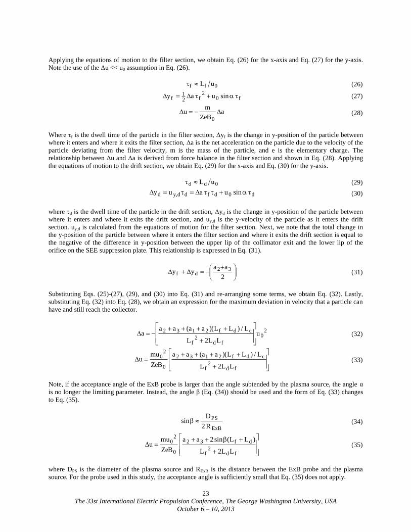
The 33st International Electric Propulsion Conference, The George Washington University, USA
October 6 – 10, 2013
23
Applying the equations of motion to the filter section, we obtain Eq. (26) for the x-axis and Eq. (27) for the y-axis.
Note the use of the Δu << u0 assumption in Eq. (26).
0ff uL (26)
f0
2f2
1f sinuay
(27)
a
ZeB
mu
0
(28)
Where f is the dwell time of the particle in the filter section, Δyf is the change in y-position of the particle between
where it enters and where it exits the filter section, Δa is the net acceleration on the particle due to the velocity of the
particle deviating from the filter velocity, m is the mass of the particle, and e is the elementary charge. The
relationship between Δu and Δa is derived from force balance in the filter section and shown in Eq. (28). Applying
the equations of motion to the drift section, we obtain Eq. (29) for the x-axis and Eq. (30) for the y-axis.
0dd uL (29)
d0dfdd,yd sinuauy
(30)
where d is the dwell time of the particle in the drift section, Δyd is the change in y-position of the particle between
where it enters and where it exits the drift section, and uy,d is the y-velocity of the particle as it enters the drift
section. uy,d is calculated from the equations of motion for the filter section. Next, we note that the total change in
the y-position of the particle between where it enters the filter section and where it exits the drift section is equal to
the negative of the difference in y-position between the upper lip of the collimator exit and the lower lip of the
orifice on the SEE suppression plate. This relationship is expressed in Eq. (31).
2
aayy 32
df (31)
Substituting Eqs. (25)-(27), (29), and (30) into Eq. (31) and re-arranging some terms, we obtain Eq. (32). Lastly,
substituting Eq. (32) into Eq. (28), we obtain an expression for the maximum deviation in velocity that a particle can
have and still reach the collector.
2
0
fd2
f
cdf2132 uLL2L
L/)LL)(aa(aaa
(32)
fd2
f
cdf2132
0
20
LL2L
L/)LL)(aa(aa
ZeB
muu
(33)
Note, if the acceptance angle of the ExB probe is larger than the angle subtended by the plasma source, the angle α
is no longer the limiting parameter. Instead, the angle β (Eq. (34)) should be used and the form of Eq. (33) changes
to Eq. (35).
ExB
PS
R2
Dsin (34)
fd2
f
df32
0
20
LL2L
)LL(sin2aa
ZeB
muu
(35)
where DPS is the diameter of the plasma source and RExB is the distance between the ExB probe and the plasma
source. For the probe used in this study, the acceptance angle is sufficiently small that Eq. (35) does not apply.
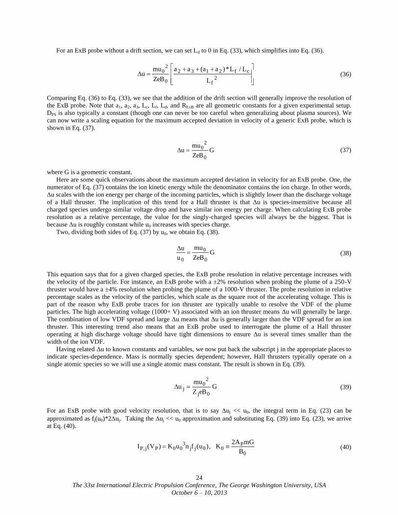
The 33st International Electric Propulsion Conference, The George Washington University, USA
October 6 – 10, 2013
24
For an ExB probe without a drift section, we can set Ld to 0 in Eq. (33), which simplifies into Eq. (36).
2f
cf2132
0
20
L
L/L*)aa(aa
ZeB
muu
(36)
Comparing Eq. (36) to Eq. (33), we see that the addition of the drift section will generally improve the resolution of
the ExB probe. Note that a1, a2, a3, Lc, Lf, Ld, and RExB are all geometric constants for a given experimental setup.
DPS is also typically a constant (though one can never be too careful when generalizing about plasma sources). We
can now write a scaling equation for the maximum accepted deviation in velocity of a generic ExB probe, which is
shown in Eq. (37).
GZeB
muu
0
20
(37)
where G is a geometric constant.
Here are some quick observations about the maximum accepted deviation in velocity for an ExB probe. One, the
numerator of Eq. (37) contains the ion kinetic energy while the denominator contains the ion charge. In other words,
Δu scales with the ion energy per charge of the incoming particles, which is slightly lower than the discharge voltage
of a Hall thruster. The implication of this trend for a Hall thruster is that Δu is species-insensitive because all
charged species undergo similar voltage drop and have similar ion energy per charge. When calculating ExB probe
resolution as a relative percentage, the value for the singly-charged species will always be the biggest. That is
because Δu is roughly constant while u0 increases with species charge.
Two, dividing both sides of Eq. (37) by u0, we obtain Eq. (38).
G
ZeB
mu
u
u
0
0
0
(38)
This equation says that for a given charged species, the ExB probe resolution in relative percentage increases with
the velocity of the particle. For instance, an ExB probe with a ±2% resolution when probing the plume of a 250-V
thruster would have a ±4% resolution when probing the plume of a 1000-V thruster. The probe resolution in relative
percentage scales as the velocity of the particles, which scale as the square root of the accelerating voltage. This is
part of the reason why ExB probe traces for ion thruster are typically unable to resolve the VDF of the plume
particles. The high accelerating voltage (1000+ V) associated with an ion thruster means Δu will generally be large.
The combination of low VDF spread and large Δu means that Δu is generally larger than the VDF spread for an ion
thruster. This interesting trend also means that an ExB probe used to interrogate the plume of a Hall thruster
operating at high discharge voltage should have tight dimensions to ensure Δu is several times smaller than the
width of the ion VDF.
Having related Δu to known constants and variables, we now put back the subscript j in the appropriate places to
indicate species-dependence. Mass is normally species dependent; however, Hall thrusters typically operate on a
single atomic species so we will use a single atomic mass constant. The result is shown in Eq. (39).
GeBZ
muu
0j
20
j (39)
For an ExB probe with good velocity resolution, that is to say uj << u0, the integral term in Eq. (23) can be
approximated as fj(u0)*2uj. Taking the uj << u0 approximation and substituting Eq. (39) into Eq. (23), we arrive
at Eq. (40).
0
P00jj
300PjP,
B
mGA2K,)u(fnuK)V(I (40)

The 33st International Electric Propulsion Conference, The George Washington University, USA
October 6 – 10, 2013
25
where K0 is a constant for a given probe design. Further substituting Eq. (24) into Eq. (40), we arrive at Eq. (41).
f023
f0
01P2j
3Pj1PjP,
DB
1K,
)DB(
KK,)VK(fVnK)V(I (41)
Where K1 and K2 are constants for a given probe design. Depending on which VDF form is in use, the associated
equation is substituted into fj, and Eq. (41) is fitted to the ExB probe trace to solve for the fitting constant. Note, Eq.
(13) is the same as Eq. (41). The formulas presented so far, though appearing in different forms, matches previously
published work.12, 27
It is the formulas to follow that are original and diverge from past work.
To calculate the species fraction and current fraction, we now need the integral equations relating each quantity
to the ExB probe collector current. To find the species fraction, we begin by re-arranging the VP3 term, then
integrating both sides of Eq. (41) with respect to VP from 0 to ∞. Since nj does not depend on VP it can go outside
the integral. The result is shown in Eq. (42). Since the integral of fj from 0 to ∞ is unity, we can further simplify the
result, which is shown in Eq. (43).
P0 3
P
Pj,PP
0P2jj1 dV
V
)V(IdV)VK(fnK
(42)
P0 3
P
Pj,P
1j dV
V
)V(I
K
1n
(43)
Equation (43) relates nj to the ExB probe collector current and can be used to calculate the species fraction. The
integration formula for species fraction is shown in Eq. (44).
k
P0 3
P
Pk,P
P0 3
P
Pj,P
k
k
jj
dVV
)V(I
dVV
)V(I
n
n (44)
To find the current fraction, we begin by relating the current of the j-th species entering the ExB probe, Ij, to the
probe collector current. The current of the j-th species is defined in Eq. (45). Substituting Eq. (24) into Eq. (45)
yields Eq. (46).
0
00j0jPjj du)u(funAeZI (45)
0
PP2jPj2
2Pjj dV)VK(fVnKAeZI
(46)
Next, we rearrange Eq. (41) by dividing both sides by VP2, then integrate both sides with respect to VP from 0 to ∞
to obtain Eq. (47). Substituting Eq. (47) into Eq. (46) yields Eq. (48).
0
P2P
PjP,
1P
0P2jPj dV
V
)V(I
K
1dV)VK(fVn (47)
0
P2P
PjP,
1
22Pj
j dVV
)V(I
K
KAeZI
(48)
Equation (48) relates Ij to the ExB probe collector current and can be used to calculate the current fraction. The
integration formula for the current fraction is shown in Eq. (49).

The 33st International Electric Propulsion Conference, The George Washington University, USA
October 6 – 10, 2013
26
k
P0 2
P
Pk,Pk
P0 2
P
Pj,Pj
k
k
jj
dVV
)V(IZ
dVV
)V(IZ
I
I (49)
B. Traditional versus new integration formulas for ExB probe analysis
Recall, the traditional approach to analyzing ExB probe data involves calculating either by geometry or by
numerical integration the area under the curve, which is assumed to be proportional to the current of the
corresponding species entering the probe. The traditional integration formula for the current fraction can be written
as Eq. (50).
k
P0
Pk,P
P0
Pj,P
k
k
jj
dV)V(I
dV)V(I
I
I (50)
While Eq. (50) is mathematically incorrect, it turns out to be a pretty good approximation of Eq. (49) for
analyzing the plume of a Hall thruster, especially when the VDF is narrow. To see why this is the case, let us
calculate the current fractions for both integration formulas in the limit of very narrow VDFs.
The current fraction calculated from the old (traditional) approach will be labeled with ΩjO and the current
fraction calculated from the new approach will be labeled with ΩjN. Assuming the incoming ion beam is composed
of species with very narrow VDFs and all charged species undergo the same voltage drop, Eq. (49) can be simplified
as shown in Eq. (51), and Eq. (50) can be simplified as shown in Eq. (52).
k
2/3kk
2/3jj
VSame
k
kkk
jjj
VDFNarrow
k
P0 2
P
Pk,Pk
P0 2
P
Pj,Pj
Nj
Zn
Zn
unZ
unZ
dVV
)V(IZ
dVV
)V(IZ
d
(51)
k
2/3kk
2/3jj
VSame
k
3kk
3jj
VDFNarrow
k
P0
Pk,P
P0
Pj,PO
jZn
Zn
un
un
dV)V(I
dV)V(I
d
(52)
The simplified expressions for the two integration approaches are equal. The voltage drop is typically very similar
between the charged species, thus any difference in the results between the new and old approaches arise mostly
from differences in the way the two approaches account for the spread in the VDF. During the present study, the
difference was found to correspond to a change in anode efficiency of only 1-2% on the average.
Acknowledgments
We thank the NASA Space Technology Mission Directorate In-Space Propulsion project for funding this work,
and Timothy D. Smith for managing the work. We thank Peter Peterson for work on the design of the NASA-300M
Hall thruster. We thank Jonathan Van Noord of the University of Michigan and Ioannis G. Mikellides of the NASA
Jet Propulsion Laboratory for work on the design of the NASA-300MS. We thank Christopher Griffith for work on
the design of both the NASA-300M and the NASA-300MS. We thank Thomas Haag for work on the thrust stand
and Daniel L. Brown and Joseph Blakely of the Air Force Research Laboratory for the retarding potential analyzer.
And we thank Kevin L. Blake, George W. Readus, George P. Jacynycz, and Thomas Raly for the thruster
fabrication, assembly of the test setup, and operation of the vacuum facility.

The 33st International Electric Propulsion Conference, The George Washington University, USA
October 6 – 10, 2013
27
References 1"NASA Exploration Systems Mission Directorate Presentation, Human Space Exploration Summary",
http://www.nasa.gov/exploration/new_space_enterprise/home/heft_summary.html, Jan., 2011. 2Mercer, C. R., et al., "Benefits of Power and Propulsion Technology for a Piloted Electric Vehicle to an Asteroid ", 47th
AIAA/ASME/SAE/ASEE Joint Propulsion Conference & Exhibit, AIAA-2011-7252, San Diego, CA, 31 Jul.- 3 Aug., 2011. 3Capadona, L. A., et al., "Feasibility of Large High-Powered Solar Electric Propulsion Vehicles: Issues and Solutions", 47th
AIAA/ASME/SAE/ASEE Joint Propulsion Conference & Exhibit, AIAA-2011-7251, San Diego, CA, 31 Jul.- 3 Aug., 2011. 4Brophy, J. R., et al., "300-kW Solar Electric Propulsion System Configuration for Human Exploration of Near-Earth Asteroids",
47th AIAA/ASME/SAE/ASEE Joint Propulsion Conference & Exhibit, AIAA-2011-5514, San Diego, CA, 31 Jul.- 3 Aug., 2011. 5Hofer, R. R. and Randolph, T. M., "Mass and Cost Model for Selecting Thruster Size in Electric Propulsion Systems", 47th
AIAA/ASME/SAE/ASEE Joint Propulsion Conference & Exhibit, AIAA-2011-5518, San Diego, CA, 31 Jul.- 3 Aug., 2011. 6Mikellides, I. G., et al., "Magnetic shielding of the channel walls in a Hall plasma accelerator", Physics of Plasmas, Vol. 18, No.
3, doi:10.1063/1.3551583, Mar. 8, 2011, pp. 033501. 7Hofer, R. R., Goebel, D. M., Mikellides, I. G., and Katz, I., "Design of a Laboratory Hall Thruster with Magnetically Shielded
Channel Walls, Phase II: Experiments", 48th AIAA/ASME/SAE/ASEE Joint Propulsion Conference & Exhibit, AIAA-2012-3788,
Atlanta, GA, 29 Jul.- 1 Aug., 2012. 8Mikellides, I. G., Katz, I., Hofer, R. R., and Goebel, D. M., "Design of a Laboratory Hall Thruster with Magnetically Shielded
Channel Walls, Phase III: Comparison of Theory with Experiment", 48th AIAA/ASME/SAE/ASEE Joint Propulsion Conference &
Exhibit, AIAA-2012-3789, Atlanta, GA, 29 Jul.- 1 Aug., 2012. 9Kamhawi, H., Haag, T. W., Jacobson, D. T., and Manzella, D. H., "Performance Evaluation of the NASA-300M 20 kW Hall
Effect Thruster", 47th AIAA/ASME/SAE/ASEE Joint Propulsion Conference & Exhibit, AIAA-2011-5521, San Diego, CA, 31
Jul.- 3 Aug., 2011. 10Kamhawi, H., et al., "Performance and Thermal Characterization of the 20 kW 300MS Hall Effect Thruster", 33rd International
Electric Propulsion Conference, 2013-444, Washington, DC, 6-10 Oct., 2013. 11Shastry, R., Huang, W., Haag, T. W., and Kamhawi, H., "Langmuir Probe Measurements within the Discharge Channel of the
20-kW NASA-300M and NASA-300MS Hall Thrusters", 33rd International Electric Propulsion Conference, 2013-122,
Washington, DC, 6-10 Oct., 2013. 12Shastry, R., Hofer, R. R., Reid, B. M., and Gallimore, A. D., "Method for analyzing ExB probe spectra from Hall thruster
plumes", Review of Scientific Instruments, Vol. 80, No. 6, doi:10.1063/1.3152218, 22 Jun., 2009, pp. 063502. 13Kim, V., "Main physical features and processes determining the performance of stationary plasma thrusters", Journal of
Propulsion and Power, Vol. 14, No. 5, 1998, pp. 736-743. 14Hofer, R. R. and Gallimore, A. D., "High-Specific Impulse Hall Thrusters, Part 2: Efficiency Analysis", Journal of Propulsion
and Power, Vol. 22, No. 4, doi:10.2514/1.15954, Jul.-Aug., 2006, pp. 732-740. 15Brown, D. L., "Investigation of Flow Discharge Voltage Hall Thruster Characteristics and Evaluation of Loss Mechanisms",
Ph.D. Dissertation, Aerospace Engineering, University of Michigan, Ann Arbor, MI, 2009. 16Reid, B. M., "The Influence of Neutral Flow Rate in the Operation of Hall Thrusters", Ph.D. Dissertation, Aerospace
Engineering, University of Michigan, Ann Arbor, MI, 2008. 17Manzella, D. M., "Scaling Hall Thrusters to High Power", Ph.D. Dissertation, Mechanical Engineering, Stanford University,
Stanford, CA, 2005. 18Hofer, R. R., Peterson, P. Y., Gallimore, A. D., and Jankovsky, R. S., "A High Specific Impulse Two-Stage Hall Thruster with
Plasma Lens Focusing", 27th International Electric Propulsion Conference, IEPC-2001-036, Pasadena, CA, 15-19 Oct., 2001. 19Hofer, R. R. and Gallimore, A. D., "The Role of Magnetic Field Topography in Improving the Performance of High-Voltage
Hall Thrusters", 38th AIAA/ASME/SAE/ASEE Joint Propulsion Conference & Exhibit, AIAA-2002-4111, Indianapolis, IN, 7-10
Jul., 2002. 20Haag, T. W., "Thrust stand for high-power electric propulsion devices", Review of Scientific Instruments, Vol. 62, No. 5,
doi:10.1063/1.1141998, May, 1991, pp. 1186. 21Lieberman, M. A. and Lichtenberg, A. J., Electrostatic Probe Diagnostics, in Principles of Plasma Discharges and Materials
Processing, 2nd ed., Ch., doi:10.1002/0471724254, Wiley, New York, 2005, pp. 185-203. 22Savitzky, A. and Golay, M. J. E., "Smoothing and Differentiation of Data by Simplified Least Squares Procedures", Analytical
Chemistry, Vol. 36, No. 8, doi:10.1021/ac60214a047, Jul., 1964, pp. 1627-1639. 23Steinier, J., Termonia, Y., and Deltour, J., "Comments on Smoothing and Differentiation of Data by Simplified Least Squares
Procedure", Analytical Chemistry, Vol. 44, No. 11, doi:10.1021/ac60319a045, Sep., 1972, pp. 1906-1909. 24Hutchinson, I. H., Principles of Plasma Diagnostics, 2nd ed., doi:10.1017/CBO9780511613630, Cambridge University Press,
2002. 25Beal, B. E., "Clustering of Hall Effect Thrusters for High-Power Electric Propulsion Applications", Ph.D. Dissertation,
Aerospace Engineering, University of Michigan, Ann Arbor, MI, 2004. 26Linnell, J. A., "An Evaluation of Krypton Propellant in Hall Thrusters", Ph.D. Dissertation, Aerospace Engineering, University
of Michigan, Ann Arbor, MI, 2007. 27Kim, S.-W., "Experimental Investigations of Plasma Parameters and Species-Dependent Ion Energy Distribution in the Plasma
Exhaust Plume of a Hall Thruster", Ph.D. Dissertation, Aerospace Engineering, University of Michigan, Ann Arbor, MI, 1999. 28Brown, D. L. and Gallimore, A. D., "Evaluation of Facility Effects on Ion Migration in a Hall Thruster Plume", Journal of
Propulsion and Power, Vol. 27, No. 3, doi:10.2514/1.B34068, May-Jun, 2011, pp. 573-585.

The 33st International Electric Propulsion Conference, The George Washington University, USA
October 6 – 10, 2013
28
29Brown, D. L. and Gallimore, A. D., "Evaluation of Ion Collection Area in Faraday probes", Review of Scientific Instruments,
Vol. 81, No. 6, doi:10.1063/1.3449541, 25 Jun., 2010, pp. 063504. 30Huang, W., Kamhawi, H., and Shastry, R., "Farfield Ion Current Density Measurements before and after the NASA HiVHAc
EDU2 Vibration Test", 48th AIAA/ASME/SAE/ASEE Joint Propulsion Conference & Exhibit, AIAA-2012-4195, Atlanta, GA, 29
Jul.- 1 Aug., 2012. 31Reid, B. M. and Gallimore, A. D., "Near-field Ion Current Density Measurements of a 6-kW Hall Thruster", 31st International
Electric Propulsion Conference, 2009-124, Ann Arbor, MI, 20-24 Sep., 2009. 32Hagstrum, H. D., "Auger Ejection of Electrons from Tungsten by Noble Gas Ions", Physical Review, Vol. 96, No. 2,
doi:10.1103/PhysRev.96.325, 15 Oct., 1954, pp. 325-335. 33Hagstrum, H. D., "Auger Ejection of Electrons from Molybdenum by Noble Gas Ions", Physical Review, Vol. 104, No. 3,
doi:10.1103/PhysRev.104.672, 1 Nov., 1956, pp. 672-683. 34Hagstrum, H. D., "Auger Ejection of Electrons from Tungsten by Noble Gas Ions", Physical Review, Vol. 104, No. 2,
doi:10.1103/PhysRev.104.317, 15 Oct., 1956, pp. 317-318. 35Hagstrum, H. D., "Metastable Ions of the Noble Gases", Physical Review, Vol. 104, No. 2, doi:10.1103/PhysRev.104.309, Sep.,
1956, pp. 309-316. 36Choueiri, E. Y., "Fundamental difference between the two Hall thruster variants", Physics of Plasmas, Vol. 8, No. 11,
doi:10.1063/1.1409344, Nov., 2001, pp. 5025-5033. 37Reid, B. M. and Gallimore, A. D., "Langmuir Probe Measurements in the Discharge Channel of a 6-kW Hall Thruster", 44th
AIAA/ASME/SAE/ASEE Joint Propulsion Conference & Exhibit, AIAA-2008-4920, Hartford, CT, 21-23 Jul., 2008.