Falling Dominoes

Steve Koellhoffer, Chana Kuhns, Karen Tsang, Mike Zeitz

December 9, 2005

The amount of time it takes for a chain of dominoes to fallvaries as a function of the number of dominoes in the chain, theamount of space between the dominoes, the total distance thedominoes span and the shape of the domino arrangement. Inthis report, we have studied falling dominoes theoretically andexperimentally in order to predict the fall time of any linear ornonlinear arrangement of falling dominoes.

1 Introduction

In certain arrangements, carbon monoxide molecules will interact with each other in sucha way that they mimic the behavior of a falling arrangement of dominoes. During a powerdisruption of any size, the disruption affects any neighbors to the source of the disruption,and in the end, it may even affect a majority of the community in which it occurs. Modelingthese type of dynamic interactions requires an understanding of a web of parts and is veryrelated to a string of colliding dominoes.

A chain of dominoes has one external force acting on it, which is the force of gravity.In a cascading system the major internal force which causes the toppling of the line is theforce of impact from one domino to the next. In our analysis of falling dominoes, we willposition the first domino so that it is in a state of unstable equilibrium. With this setup,we can neglect all other external forces so it will be the only force acting on the dominoes.In our study, we have examined the system’s energy to develop a theoretical model for thetoppling domino chain. We have also validated our theoretical models by comparing themto experimental data. Using both these mathematical and experimental techniques, we havedeveloped a final model that predicts the toppling time of the line of dominoes.

2 Objectives

Studying topple time is the “big picture” of this project. In particular, we have completedthe following challenges:

1

• Predict the topple time of an arrangement of dominoes–both linear and nonlinear,equal spacing and nonequal spacing.

• Given a fixed distance L, construct a domino setup that minimizes topple time.

• Predict the topple time of other groups’ dominoes arrangement.

• Given a fixed distance L and N dominoes, construct a setup that minimizes toppletime.

3 Theory

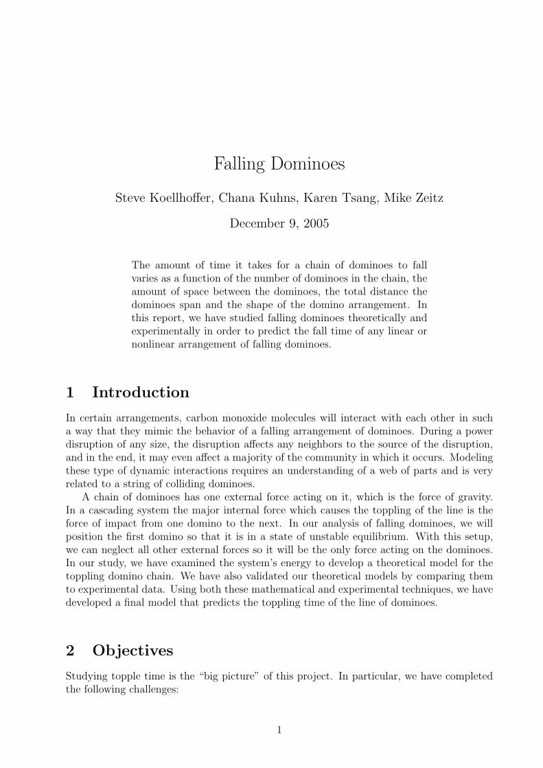
To begin creating our model, we first defined our parameters, variables and assumptions.We labeled the major dimensions of our system as in Figure 1, with w as the width of thedomino, h as the height of the domino and t as the thickness of the domino. Additionally,

Figure 1: Domino Labels

we defined L as the distance from the front of one domino to the next domino, N as thenumber of dominoes and D as the total distance the dominoes span.

We made the the following assumptions to simplify our cascading domino system:

• All of the dominoes are uniform in size and mass. In order to simplify ourcalculations, we assumed all the dominoes have the same dimensions and masses. Inparticular, we used the average height, width, thickness, and mass of the 60 dominoeswe measured.

• Dominoes will not slip about their bottom edge, creating a pivot pointwhich will remain in contact throughout its fall. Throughout the experiments,the dominoes fell on a sandpaper surface, which ensured that this assumption is true.

• Each domino will strike the successive domino once and only once and slidethrough the contact region (Stronge, Wave of Destabilizing). This allowed us toeliminate a double impact from one domino to the next which simplified our problemin its early stages.

2

• Conservation of energy. We assumed energy is conserved throughout the topplingof the line of dominoes. This allowed us to neglect frictional losses from dominoessliding as well as losses to air resistance.

• Conservation of angular momentum. The angular velocity will be directly pro-portional one domino to the next through impact.

• Initial angular velocity is ZERO. The launching device that we built ensured thatthe initial angular velocity of the first domino was insignificant and no initial kineticenergy was added to the system.

To solve the problem of minimizing topple time, our team examined several differentapproaches. Each of these will later be compared to our experimental results to see whichmodels the real system the best.

The first technique we tried was maximizing the initial torque of a single domino hittingthe next domino in a two domino system. We simplified our system so that this techniquewould be applicable to an entire system regardless of the number of dominoes behind andin front of the two domino system. The cascading line is essentially a unlimited number oftwo object collisions.

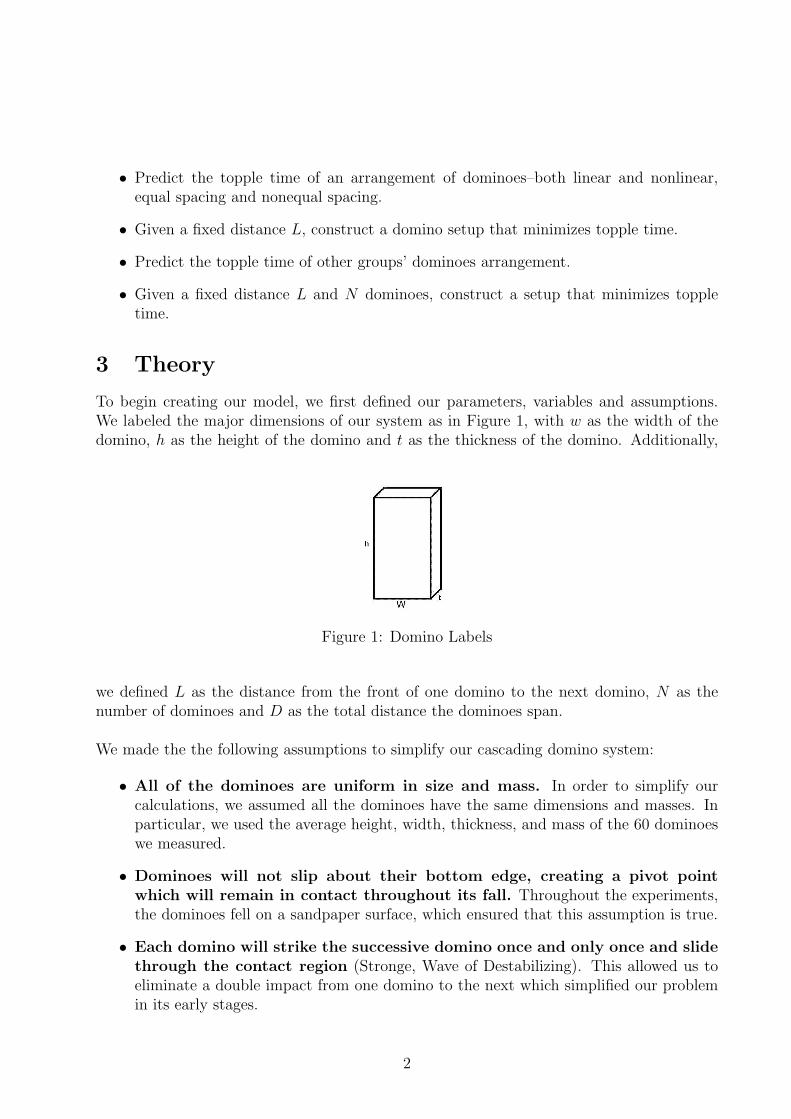
The most important part of this process was defining the geometries of the system (seeFigure 2). The force of gravity, mg, acted directly at the center of mass of each of the twodominoes. In our system, h is the height of a single domino, t is the thickness, R is theinitial distance from the point of contact to the pivot point, y is the initial height from thebottom of the domino and the angles were defined as follows:

θ = cos(s/h) (1)

γ = tan(y/t) (2)

where y = h sin(θ).

Figure 2: Domino Variables

An equation for the moment imposed on domino 2 by domino 1 was created and modifiedso that it was only as a function of θ. The underlying equation for the moment on a rigidobject is defined as

3

M = RXF, (3)

where M is the moment in newton-meters, R is the distance from the force contact to thepivot point and F is the force in newtons. The RHS of the equation can be modified froma cross product into the form

M = R ∗ FR, (4)

where FR is the component of the force acting perpendicular to R. This component of theforce can be written as

FR = F sin(φ), (5)

with the angle φ = π2− (π− θ− γ). By taking the moment about the point A, we can solve

for the moment that will be acting on the second domino by the first domino.

ΣMA = mg sin(θ)h

2−mg cos(θ)

t

2− Fh (6)

and can be simplified to

F =mg(sin(θ)h− cos(θ)t)

2h. (7)

We can now write the moment equation about the pivot point of the second domino.

ΣMB = RF sin(φ) (8)

where R = h sin(θ)sin(γ)

and γ = tan(h sin(θ)t

). The moment equation now becomes

ΣMB =h sin(θ)

sin(tan(h sin(θ)t

))

mg(h sin(θ)− t cos(θ))

2hsin[

π

2− (π − θ − tan(

h sin(θ)

t))]. (9)

We can find the maximum moment by plotting the function or by finding when the derivativeis equal to zero. Solving for this gives us an angle of θt =1.37 radians=78.5 degrees. Using(1) we can solve for s + t to be

0.867cm + 0.679cm = 1.55cm (10)

to measure the front to front spacing of our domino line. This equal linear spacing will betested in our experimental section to evaluate the theory.

The second technique we used to examine our spacing model was based upon the Strongestudy in ‘The Domino Effect’ in which he was able to create a trend for the intrinsic angularspeed of the domino cascade. They examined a set of linearly spaced dominoes and wereable to solve for a natural propagation speed of the line. They created a set of trend linesfor angular speed as a function of the ratio of the width over the height and the spacing overthe height. The results of his study are shown in Figure 3.

4

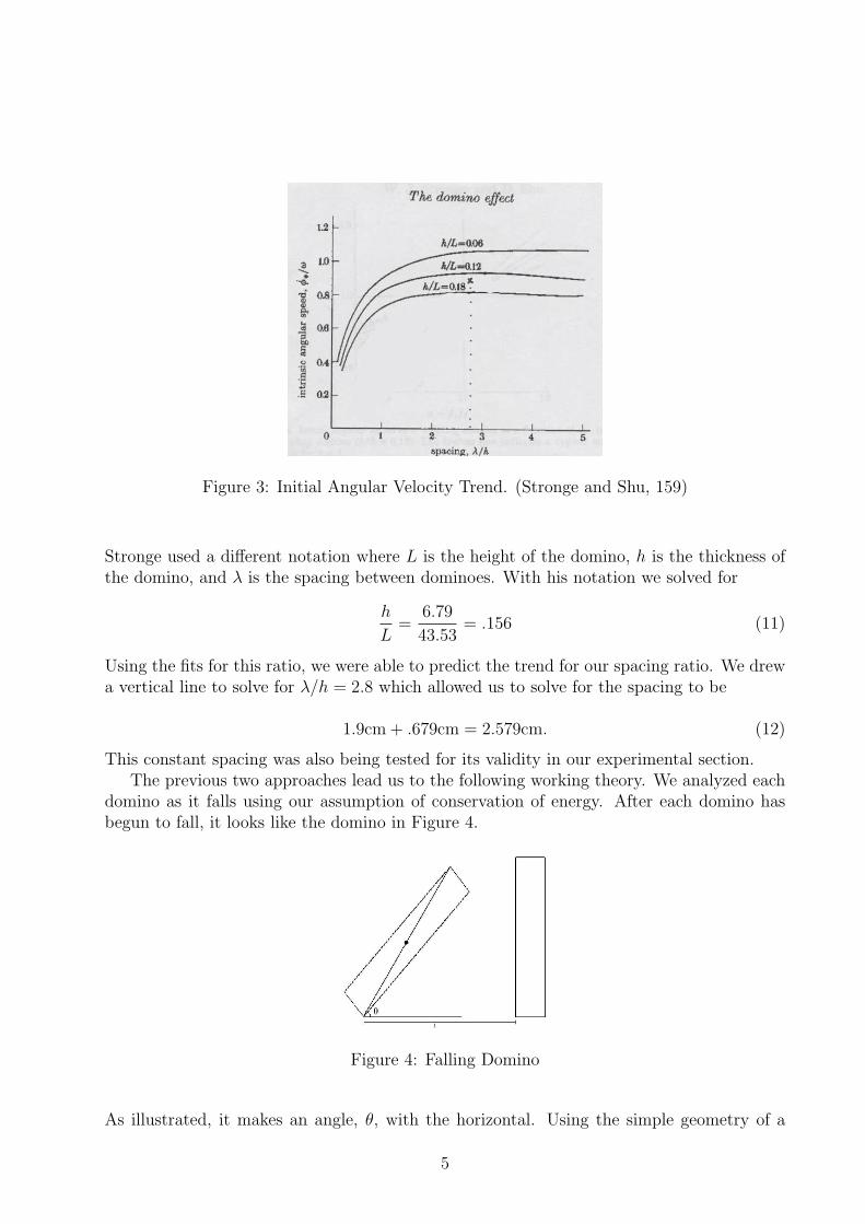
Figure 3: Initial Angular Velocity Trend. (Stronge and Shu, 159)

Stronge used a different notation where L is the height of the domino, h is the thickness ofthe domino, and λ is the spacing between dominoes. With his notation we solved for

h

L=

6.79

43.53= .156 (11)

Using the fits for this ratio, we were able to predict the trend for our spacing ratio. We drewa vertical line to solve for λ/h = 2.8 which allowed us to solve for the spacing to be

1.9cm + .679cm = 2.579cm. (12)

This constant spacing was also being tested for its validity in our experimental section.The previous two approaches lead us to the following working theory. We analyzed each

domino as it falls using our assumption of conservation of energy. After each domino hasbegun to fall, it looks like the domino in Figure 4.

Figure 4: Falling Domino

As illustrated, it makes an angle, θ, with the horizontal. Using the simple geometry of a

5

Figure 5: Geometry of Falling Domino

falling domino, as demonstrated by Figure 5, we determined that as the domino falls, itspotential energy is

U = mg(t

2cos θ +

h

2sin θ), (13)

and its kinetic energy is

T =1

2mv2 +

1

2Iθ̇2, (14)

where I, the domino’s moment of inertia about its center of mass, and v, its tangentialvelocity at its center of mass, are as follows:

I =1

12m(h2 + t2) (15)

v =d

2θ̇. (16)

Figure 6: Any Domino that Begins to Topple

6

Using these values and solving once more for T , we get:

T =1

6mθ̇2(h2 + t2). (17)

So, the total energy for the falling domino is E = U + T , or

E = mg(t

2cos θ +

h

2sin θ) +

1

6mθ̇2(h2 + t2)). (18)

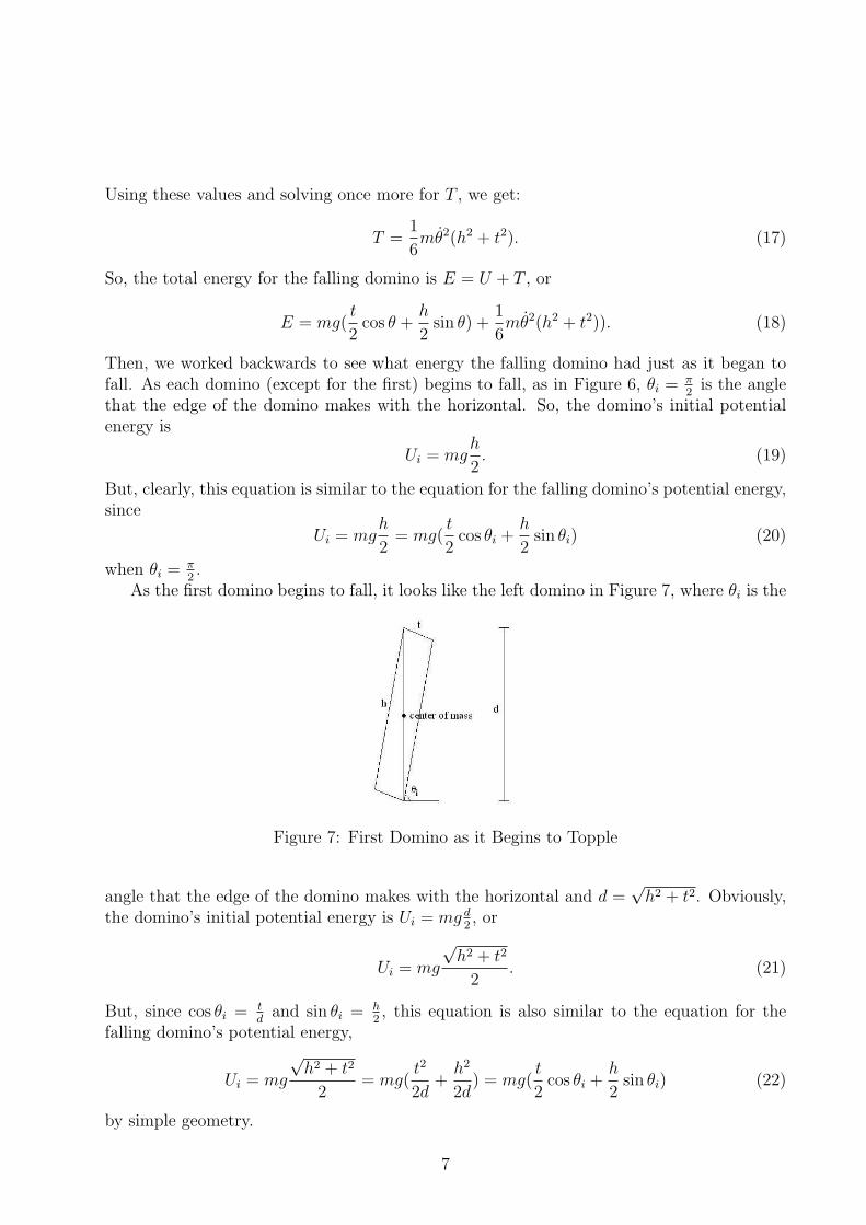
Then, we worked backwards to see what energy the falling domino had just as it began tofall. As each domino (except for the first) begins to fall, as in Figure 6, θi = π

2is the angle

that the edge of the domino makes with the horizontal. So, the domino’s initial potentialenergy is

Ui = mgh

2. (19)

But, clearly, this equation is similar to the equation for the falling domino’s potential energy,since

Ui = mgh

2= mg(

t

2cos θi +

h

2sin θi) (20)

when θi = π2.

As the first domino begins to fall, it looks like the left domino in Figure 7, where θi is the

Figure 7: First Domino as it Begins to Topple

angle that the edge of the domino makes with the horizontal and d =√

h2 + t2. Obviously,the domino’s initial potential energy is Ui = mg d

2, or

Ui = mg

√h2 + t2

2. (21)

But, since cos θi = td

and sin θi = h2, this equation is also similar to the equation for the

falling domino’s potential energy,

Ui = mg

√h2 + t2

2= mg(

t2

2d+

h2

2d) = mg(

t

2cos θi +

h

2sin θi) (22)

by simple geometry.

7

Next, we realized that the kinetic energy was exactly the same for any domino as it beginsto fall, namely

Ti =1

2mv2

i +1

2Iθ̇i

2(23)

where I, the domino’s moment of inertia about its center of mass, is the same as above andvi, its tangential velocity at its center of mass, is as follows

vi =d

2θ̇i. (24)

Plugging vi and I into the equation, it is easy to see that the domino’s kinetic energy is

Ti =1

6mθ̇i

2(h2 + t2). (25)

However, one of our assumptions is that θ̇i is negligible for the first domino. So, Equation13 only holds for the first domino assuming θ̇i = 0 for the first domino.

Subsequently, we combined our theory and found that for any domino, the total initialenergy, Ei = Ui + Ti, and so

Ei = mg(t

2cos θi +

h

2sin θi) +

1

6mθ̇2(h2 + t2). (26)

Finally, we applied our assumption that energy is conserved in the system, so that for eachdomino, Ei = E. Solving this equation for θ̇, we got a separable first order differentialequation:

θ̇ = −√

θ2i +

3g

h2 + t2(h(sin θi − sinθ)− t(cos θi − cosθ)). (27)

The above equation applies to the first domino with θi as it was measured in our experiments.

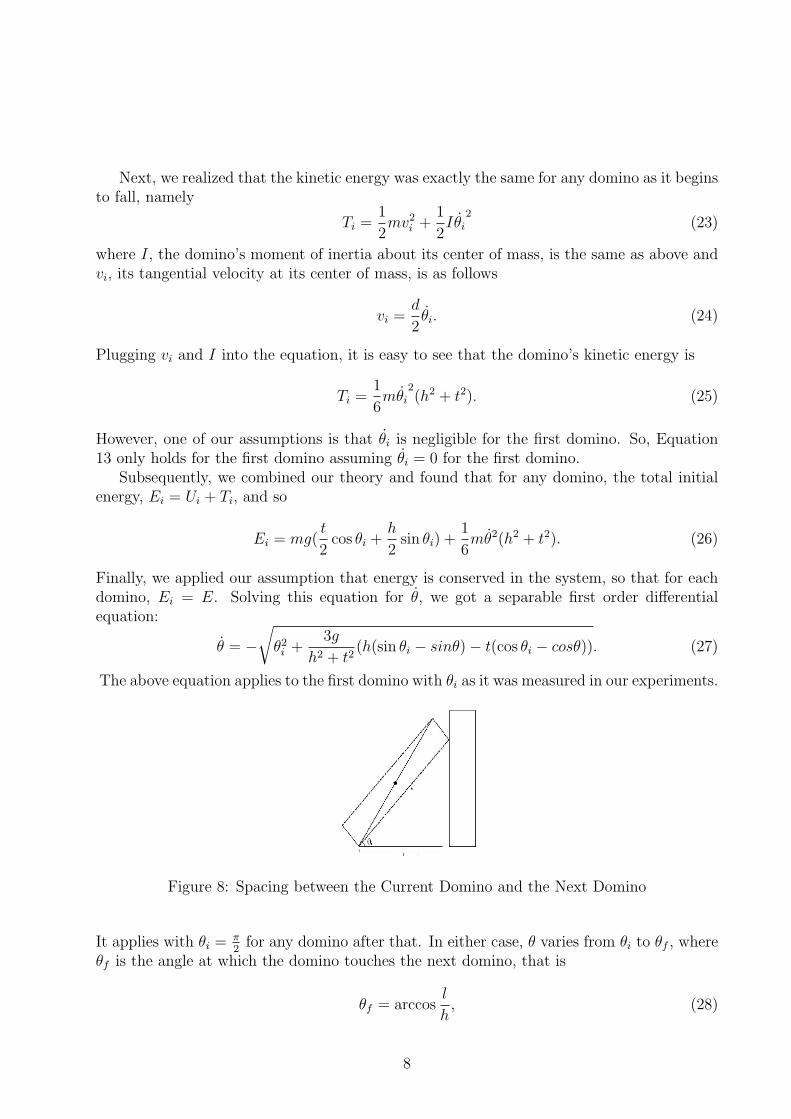
Figure 8: Spacing between the Current Domino and the Next Domino

It applies with θi = π2

for any domino after that. In either case, θ varies from θi to θf , whereθf is the angle at which the domino touches the next domino, that is

θf = arccosl

h, (28)

8

where l is the spacing between the current domino and the next domino, as shown in Figure8.

In order to use Equation (27) it became essential that we know the initial angular velocityof each domino. To obtain this we assumed that the initial angular velocity of a dominois equal to the final velocity of the previous domino multiplied by a scaling term e. Thescaling term e is a dimensionless number that is a function of the ratio of domino spacingto domino height, so e = e( l

h). Therefore, ˙θi2 = e ˙θf1. To determine the function for e, we

looked at our experimental results and found the number for e that yielded the most accuratetime predictions. After obtaining e from 31 different experiments, a graph of e vs. l

hwas

constructed (see Figure 9).

Figure 9: Experimental Scaling Terms

There appeared to be a quadratic trend to the data so we fitted a second order polynomialto the data with moderate success, R2 = 0.7027. The equation for e we found was:

e = −2.9098(l

h)2 + 3.4744

l

h− 0.3987. (29)

To predict the fall time for any domino arrangements, we created a Maple worksheet (SeeAppendix A) that determines fall time of a set of dominoes based on the number of dominoesand the spacing between them. Once the relevant spacings are input, e is calculated from ourfit, and then the time it takes for each domino to get from its starting position to the nextdomino (or the ground in the case of the final domino) is determined and added together toobtain the total fall time.

A supplemental theory was generated so that our linear theory could also predict curveddomino cascade setups. Using AutoCAD we input the given curved setup from an overhead

9

view so that it was possible to see the width and thickness of each domino. The correctdimensional values of each domino gave an exact position of each in space while in theupright position. The position of each domino is defined by the spacing and angle from theprevious domino. The position of the first domino is relative and the rest of the dominoescan be set up accordingly.

The positives of using a CAD tool in our experiments allows us to input accurate lengthsand angles and get an overall picture of the setup. Our linear calculation used the averagespacing between dominoes to find the angle of collision and our velocity transfer coefficient.To predict the dynamics of a linear string of dominoes, we used the distance from front tofront of each domino as the spacing. For our curved experiments, we tried using severaldifferent distances from one domino to the next. With the CAD setup (See Figure 10) wecould easily find the distance between each center to center, contact points and corner tocorner using either closest or farthest corners. Each of these spacing methods was used topredict the fall time and compared. For each of the three measurement techniques we triedusing individual spacing as well as average spacing in our model to predict the time.

Figure 10: CAD Setup for Spacing and Angle Measurements

After calculating the predictive model time we found that the actual time appeared tobe a factor related to the total rotational angle of the dominoes. We generated a non-dimensional scaling factoring based upon the sum of the absolute value of the relative anglechanges. It was also important for our curve theory to be continuous with our linear theoryso that when the angle of change was zero the scaling factor would be one and not affect theresult. This resulted in the following equation:

t ∗ (1 + frac(Σ|θ|)360), (30)

where t is the predicted time from our model and Σ|θ| is the sum of the absolute valuesof the angles of the dominoes as measured parallel to the previous domino. This scalingmechanism allows the time predicted to be a continuous function when moving from linear

10

to nonlinear strings of dominoes. Thus, the fall time for a linear string of dominoes remainsthe same when θ is 0 and the time will increase when dominoes are not parallel.

4 Experiments and Results

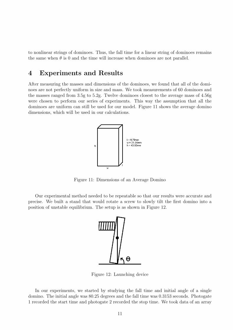
After measuring the masses and dimensions of the dominoes, we found that all of the domi-noes are not perfectly uniform in size and mass. We took measurements of 60 dominoes andthe masses ranged from 3.5g to 5.2g. Twelve dominoes closest to the average mass of 4.56gwere chosen to perform our series of experiments. This way the assumption that all thedominoes are uniform can still be used for our model. Figure 11 shows the average dominodimensions, which will be used in our calculations.

Figure 11: Dimensions of an Average Domino

Our experimental method needed to be repeatable so that our results were accurate andprecise. We built a stand that would rotate a screw to slowly tilt the first domino into aposition of unstable equilibrium. The setup is as shown in Figure 12.

Figure 12: Launching device

In our experiments, we started by studying the fall time and initial angle of a singledomino. The initial angle was 80.25 degrees and the fall time was 0.3153 seconds. Photogate1 recorded the start time and photogate 2 recorded the stop time. We took data of an array

11

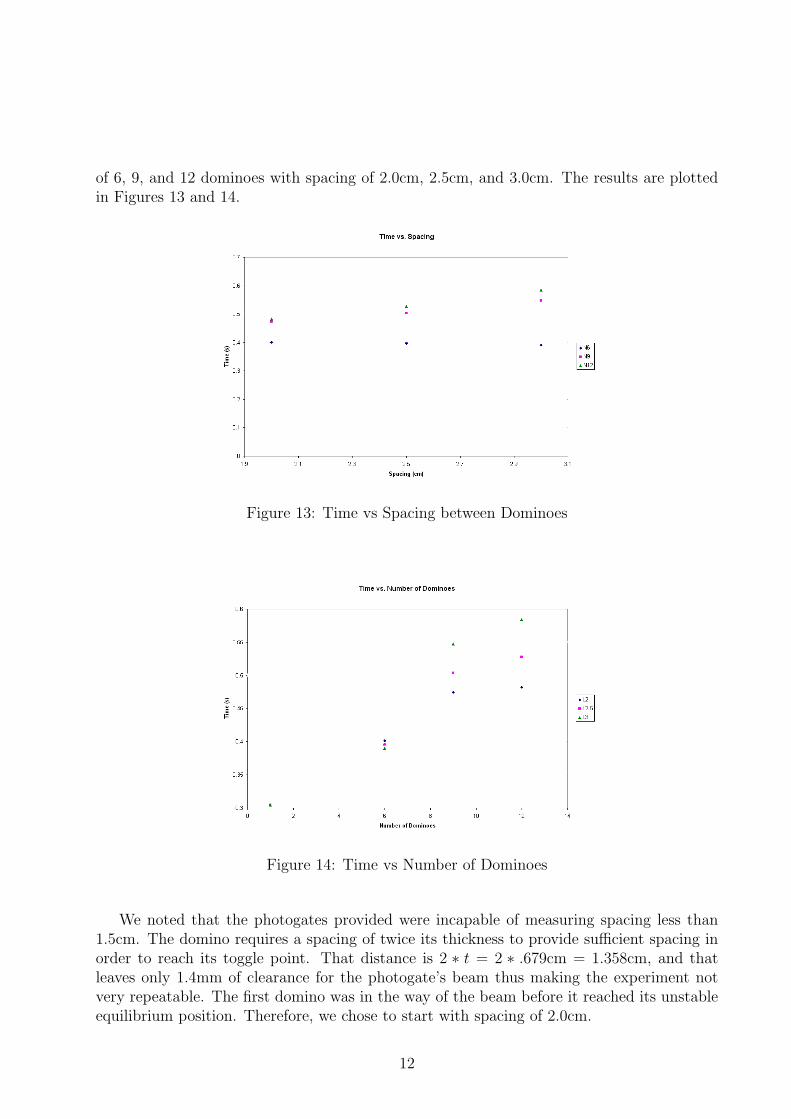
of 6, 9, and 12 dominoes with spacing of 2.0cm, 2.5cm, and 3.0cm. The results are plottedin Figures 13 and 14.

Figure 13: Time vs Spacing between Dominoes

Figure 14: Time vs Number of Dominoes

We noted that the photogates provided were incapable of measuring spacing less than1.5cm. The domino requires a spacing of twice its thickness to provide sufficient spacing inorder to reach its toggle point. That distance is 2 ∗ t = 2 ∗ .679cm = 1.358cm, and thatleaves only 1.4mm of clearance for the photogate’s beam thus making the experiment notvery repeatable. The first domino was in the way of the beam before it reached its unstableequilibrium position. Therefore, we chose to start with spacing of 2.0cm.

12

It took many trials and much practice before getting consistent data. Setting up the row,the photogates and initiating the fall proved to be very time consuming. If one of the trialsseemed to be an outlier compared to other tests, we removed it from our data section.

After much experimentation using photogates, we determined that the results reliedheavily on how the first photogate (measuring start time) was positioned. So, we decidedto use a high-speed camera to record the fall time of dominoes. We modified our launchingdevice a little bit to adapt to the change in equipment. Our team first glued sandpaper on

Figure 15: New Setup with Modified Launching Device

a piece of wooden board. The sandpaper is completely attached to the board to achieve aflat surface. We then taped a ruler on top of the sandpaper for placement of dominoes. Thelaunching device is then clamped to the board. Figure 15 illustrates the new setup.

We noticed that there was a lot of room for error when deciding the time the dominoleaves the screw, so we sharpened the end of the screw, so that the tip is pointy. With thepointy tip, it’s easier to tell when the domino leaves the screw. There was also a problemwith dark colored dominoes because they did not reflect light as well as the lighter coloredones, so we eliminated the darker ones from our experiments.

In setting up the software, we used 1000 frames/second frame rate, shutter speed of1/5000 second, and a resolution of 512x512. The video of falling dominoes was capturedunder these settings. A sample frame is shown in Figure 16.

Figure 16: Sample Frame taken with High Speed Camera

The next step was to review the video to determine the time the first domino left thescrew and the time the last domino hits the ground. We paused the video near the point

13

when the first domino was leaving the screw. We then changed the frame rate to the slowestsetting and zoomed in to view movements in “pixel” details. Therefore, we were able todetermine the instant when the first domino left the screw. After we recorded the start time,we fast-forwarded the video to the instant before the last domino hit the board. We wantedto find the first frame that the last domino became parallel to the board. We had to becareful, because much of the time the last domino bounced against the board at least once.We then record the first instant the last domino was parallel to the board as the stop time.The difference of the start time and stop time gave us the fall time that we are interested in.

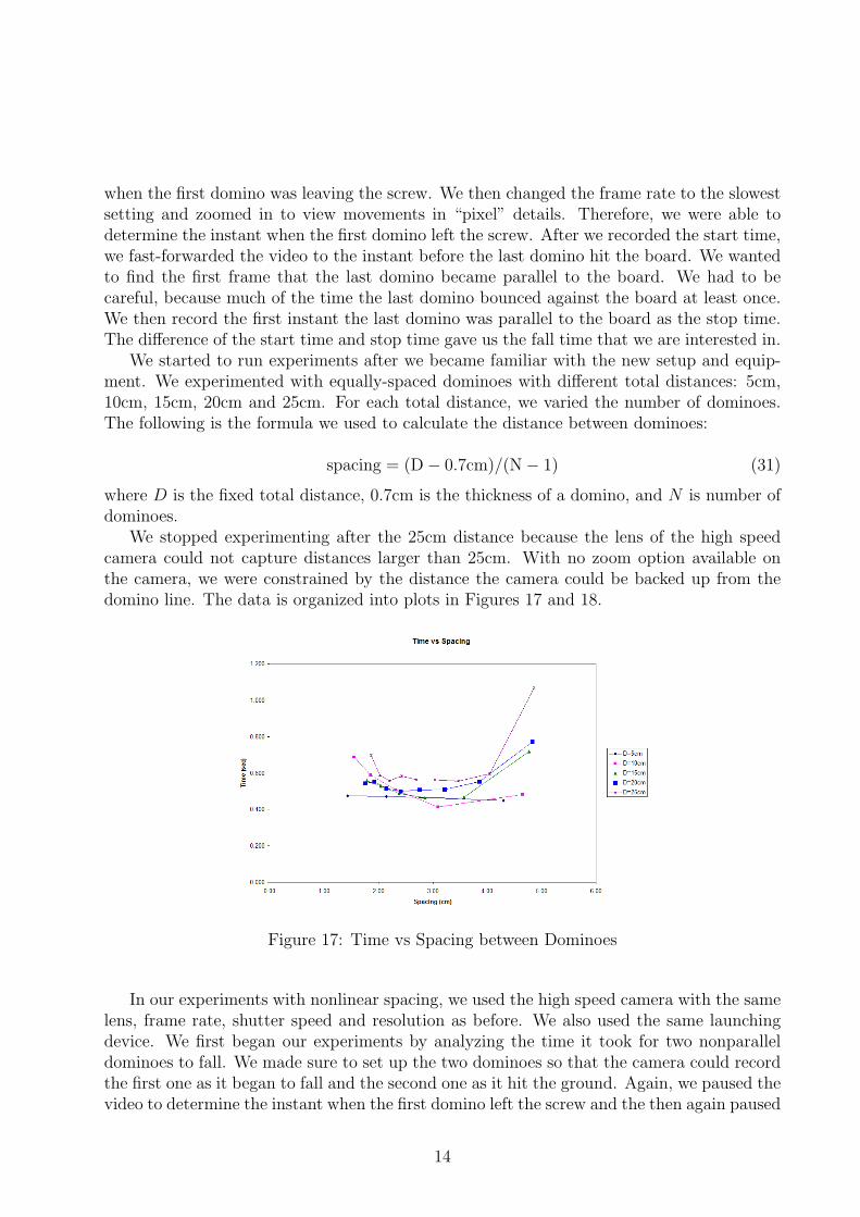
We started to run experiments after we became familiar with the new setup and equip-ment. We experimented with equally-spaced dominoes with different total distances: 5cm,10cm, 15cm, 20cm and 25cm. For each total distance, we varied the number of dominoes.The following is the formula we used to calculate the distance between dominoes:

spacing = (D− 0.7cm)/(N− 1) (31)

where D is the fixed total distance, 0.7cm is the thickness of a domino, and N is number ofdominoes.

We stopped experimenting after the 25cm distance because the lens of the high speedcamera could not capture distances larger than 25cm. With no zoom option available onthe camera, we were constrained by the distance the camera could be backed up from thedomino line. The data is organized into plots in Figures 17 and 18.

Figure 17: Time vs Spacing between Dominoes

In our experiments with nonlinear spacing, we used the high speed camera with the samelens, frame rate, shutter speed and resolution as before. We also used the same launchingdevice. We first began our experiments by analyzing the time it took for two nonparalleldominoes to fall. We made sure to set up the two dominoes so that the camera could recordthe first one as it began to fall and the second one as it hit the ground. Again, we paused thevideo to determine the instant when the first domino left the screw and the then again paused

14

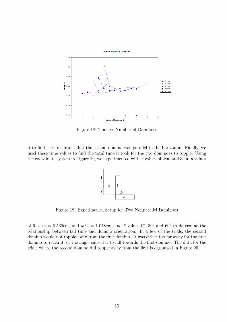
Figure 18: Time vs Number of Dominoes

it to find the first frame that the second domino was parallel to the horizontal. Finally, weused these time values to find the total time it took for the two dominoes to topple. Usingthe coordinate system in Figure 19, we experimented with x values of 2cm and 3cm, y values

Figure 19: Experimental Setup for Two Nonparallel Dominoes

of 0, w/4 = 0.539cm, and w/2 = 1.078cm, and θ values 0o, 30o and 60o to determine therelationship between fall time and domino orientation. In a few of the trials, the seconddomino would not topple away from the first domino. It was either too far away for the firstdomino to reach it, or the angle caused it to fall towards the first domino. The data for thetrials where the second domino did topple away from the first is organized in Figure 20.

15

Figure 20: Fall Times for 2 Domino Orientation Experiment

From this data no explicit trend is obvious. This is due to the many sources or errorinvolved, mainly the non-uniformity of the dominoes. However, in general time increaseswith both y and θ.

Next, we set up experiments with curves of dominoes. Again, we made sure that althoughthe curves were nonlinear, the first domino was recorded as it began to fall and the lastdomino in the arrangement was recorded as it hit the ground. To organize our experimentswith more than two dominoes, we set up a different coordinate system with the spacingand angle from one domino to the next as in Figure 21. Using these coordinates, we

Figure 21: Experimental Setup for More Than Two Dominoes with Nonlinear Spacing

tested four semicircular domino arrangements and two undulating domino arrangements.The semicircular arrangements had the spacings and angles between consecutive dominoesand fall times in Figure 22. The undulating arrangements looked similar to the one in Figure23.

16

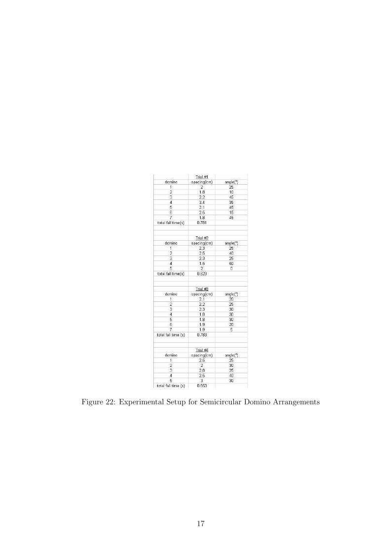
Figure 22: Experimental Setup for Semicircular Domino Arrangements

17

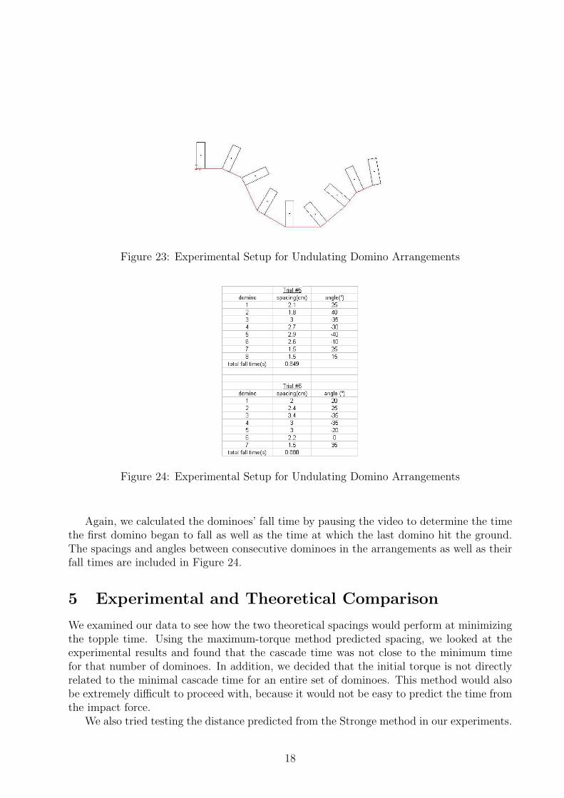
Figure 23: Experimental Setup for Undulating Domino Arrangements

Figure 24: Experimental Setup for Undulating Domino Arrangements

Again, we calculated the dominoes’ fall time by pausing the video to determine the timethe first domino began to fall as well as the time at which the last domino hit the ground.The spacings and angles between consecutive dominoes in the arrangements as well as theirfall times are included in Figure 24.

5 Experimental and Theoretical Comparison

We examined our data to see how the two theoretical spacings would perform at minimizingthe topple time. Using the maximum-torque method predicted spacing, we looked at theexperimental results and found that the cascade time was not close to the minimum timefor that number of dominoes. In addition, we decided that the initial torque is not directlyrelated to the minimal cascade time for an entire set of dominoes. This method would alsobe extremely difficult to proceed with, because it would not be easy to predict the time fromthe impact force.

We also tried testing the distance predicted from the Stronge method in our experiments.

18

We found that the time exceeded the minimum experimental time. We can also understandthat the intrinsic angular velocity may not be directly related to the maximum linear cascad-ing velocity. In addition, Stronge’s technique does not consider nonconstant spacing. Thistype of setup may perhaps be the best way to minimize the topple time over a distance.

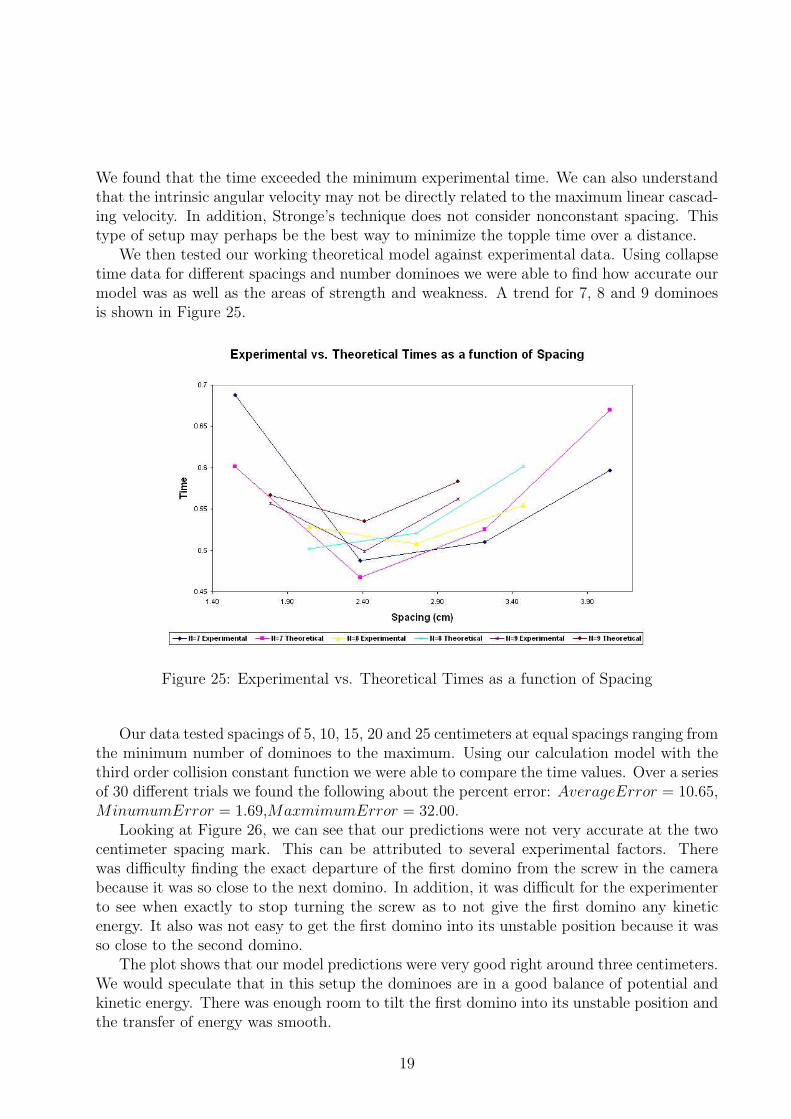
We then tested our working theoretical model against experimental data. Using collapsetime data for different spacings and number dominoes we were able to find how accurate ourmodel was as well as the areas of strength and weakness. A trend for 7, 8 and 9 dominoesis shown in Figure 25.

Figure 25: Experimental vs. Theoretical Times as a function of Spacing

Our data tested spacings of 5, 10, 15, 20 and 25 centimeters at equal spacings ranging fromthe minimum number of dominoes to the maximum. Using our calculation model with thethird order collision constant function we were able to compare the time values. Over a seriesof 30 different trials we found the following about the percent error: AverageError = 10.65,MinumumError = 1.69,MaxmimumError = 32.00.

Looking at Figure 26, we can see that our predictions were not very accurate at the twocentimeter spacing mark. This can be attributed to several experimental factors. Therewas difficulty finding the exact departure of the first domino from the screw in the camerabecause it was so close to the next domino. In addition, it was difficult for the experimenterto see when exactly to stop turning the screw as to not give the first domino any kineticenergy. It also was not easy to get the first domino into its unstable position because it wasso close to the second domino.

The plot shows that our model predictions were very good right around three centimeters.We would speculate that in this setup the dominoes are in a good balance of potential andkinetic energy. There was enough room to tilt the first domino into its unstable position andthe transfer of energy was smooth.

19

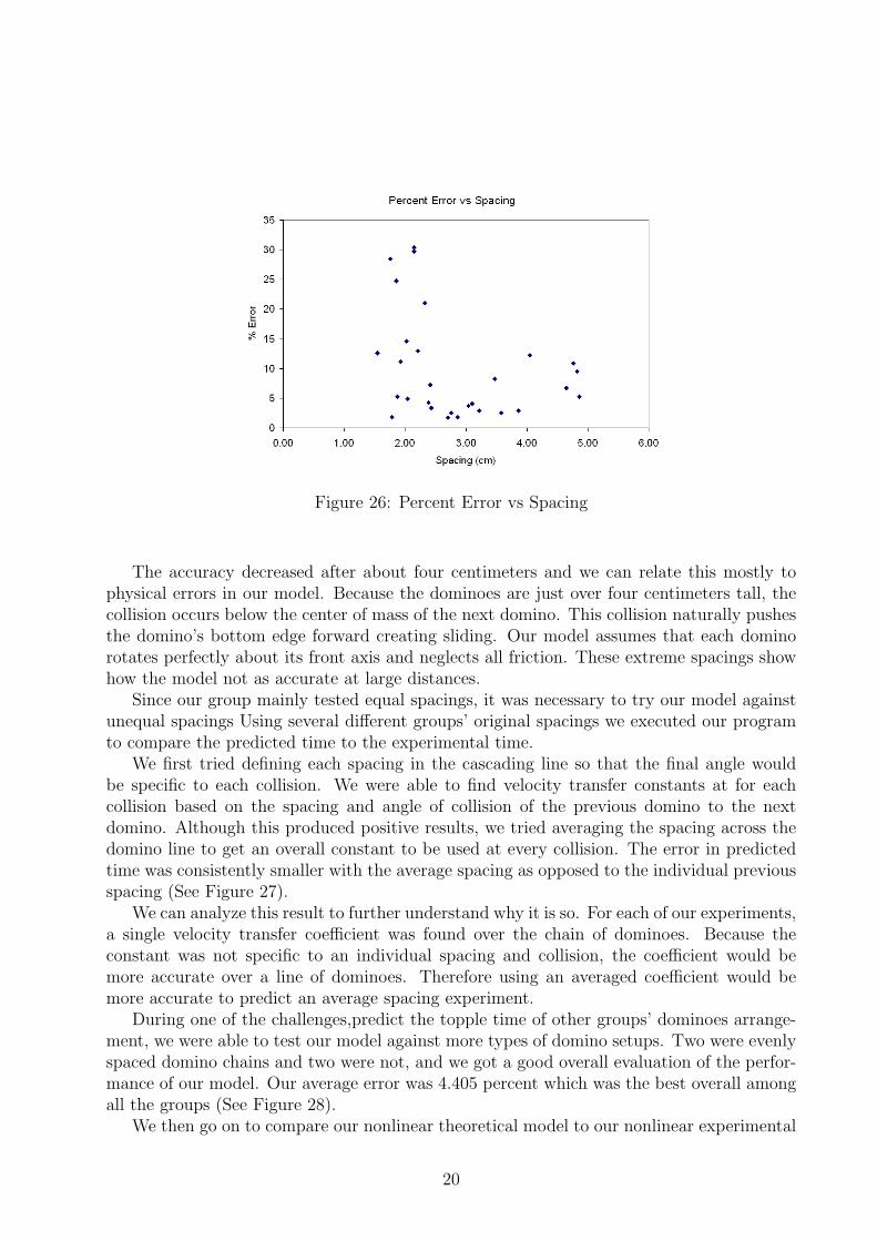
Figure 26: Percent Error vs Spacing

The accuracy decreased after about four centimeters and we can relate this mostly tophysical errors in our model. Because the dominoes are just over four centimeters tall, thecollision occurs below the center of mass of the next domino. This collision naturally pushesthe domino’s bottom edge forward creating sliding. Our model assumes that each dominorotates perfectly about its front axis and neglects all friction. These extreme spacings showhow the model not as accurate at large distances.

Since our group mainly tested equal spacings, it was necessary to try our model againstunequal spacings Using several different groups’ original spacings we executed our programto compare the predicted time to the experimental time.

We first tried defining each spacing in the cascading line so that the final angle wouldbe specific to each collision. We were able to find velocity transfer constants at for eachcollision based on the spacing and angle of collision of the previous domino to the nextdomino. Although this produced positive results, we tried averaging the spacing across thedomino line to get an overall constant to be used at every collision. The error in predictedtime was consistently smaller with the average spacing as opposed to the individual previousspacing (See Figure 27).

We can analyze this result to further understand why it is so. For each of our experiments,a single velocity transfer coefficient was found over the chain of dominoes. Because theconstant was not specific to an individual spacing and collision, the coefficient would bemore accurate over a line of dominoes. Therefore using an averaged coefficient would bemore accurate to predict an average spacing experiment.

During one of the challenges,predict the topple time of other groups’ dominoes arrange-ment, we were able to test our model against more types of domino setups. Two were evenlyspaced domino chains and two were not, and we got a good overall evaluation of the perfor-mance of our model. Our average error was 4.405 percent which was the best overall amongall the groups (See Figure 28).

We then go on to compare our nonlinear theoretical model to our nonlinear experimental

20

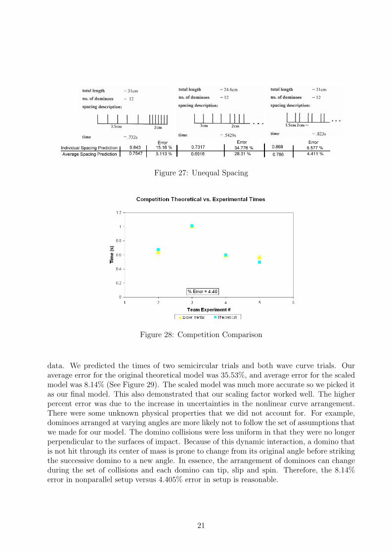
Figure 27: Unequal Spacing

Figure 28: Competition Comparison

data. We predicted the times of two semicircular trials and both wave curve trials. Ouraverage error for the original theoretical model was 35.53%, and average error for the scaledmodel was 8.14% (See Figure 29). The scaled model was much more accurate so we picked itas our final model. This also demonstrated that our scaling factor worked well. The higherpercent error was due to the increase in uncertainties in the nonlinear curve arrangement.There were some unknown physical properties that we did not account for. For example,dominoes arranged at varying angles are more likely not to follow the set of assumptions thatwe made for our model. The domino collisions were less uniform in that they were no longerperpendicular to the surfaces of impact. Because of this dynamic interaction, a domino thatis not hit through its center of mass is prone to change from its original angle before strikingthe successive domino to a new angle. In essence, the arrangement of dominoes can changeduring the set of collisions and each domino can tip, slip and spin. Therefore, the 8.14%error in nonparallel setup versus 4.405% error in setup is reasonable.

21

Figure 29: Theoretical and Experimental Error Comparison

6 Conclusion

The dynamic analysis and prediction of a cascading line of dominoes is a very difficult. Byfirst simplifying the problem, we set up a number of assumptions to help us proceed intodeveloping a model. We experimentally and theoretically studied a single falling dominoreleased from its unstable position. Our team developed an energy equation based upon thebalance of kinetic and potential energy. After understanding the topple of a single domino,we expanded this model to a system of dominoes cascading through collisions.

Our team first used experimental data to create a mathematical prediction of time of alinear chain as a function of spacing and number of dominoes. This theory was inaccurateat nonconstant spacing so we developed a new model using a velocity transfer coefficientfrom one domino to the next. This coefficient was a function of a dimensionless parameterof spacing/height and was found using experimental data.

The next step was to expand the theory so that we could predict falling time for curvedarrangements. An additional scaling constant was used to account for the increase in fallingtime due to collisions at various angles. This constant enabled our mathematical model tobe continuous across both linear and curved arrangements.

The evolution of our theory developed to account for numerous domino arrangements.Our methods have been very successful in determining the fall time of a chain of dominoes.

7 Annotated Bibliography

Banks, R. B. (1998). Towing Icebergs, Falling Dominoes, and other Adventures in AppliedMathematics. Princeton, Princeton University Press.

22

Banks looks to examine mainly the ‘wave motion’ that is associated with cascadingdominoes. First, a individual slender object is studied with a frictionless axle at the basethat is free to rotate, neglecting air resistance. Conservation of energy yields the relationbetween potential and kinetic energy of the system. The equation is modified into a formthat will find the time for the pole to fall over. He adds that it is necessary to give a nudgeto create a small angular velocity on the object, which is part of the equation.

He similarly examines a wave of dominoes spaced evenly apart. He makes the assumptionthat “only one domino affects the next one in the row” and the preceding three or four leaningdominoes are neglected. After some manipulation he forms the equation that gives the timeof fall of the wave.

Our initial model will be similar to that of Banks, but we hope to expand to include alldominoes that have any dynamic effect on the system. Still, his model is a good place tostart in that he makes several rational simplifications to create a rough model.

Bert,C. W. (1986). “Falling Dominoes.” SIAM Review 28(2): 219-224.

This paper will be very useful as a preliminary guide when investigating the mechanicsof falling dominoes. The author uses the following assumptions:

• All dominoes are identical.

• The dominoes are parallel to each other and equally spaced.

• There is no sliding of the dominoes on the plane and each domino remains in contactwith the plane at least along one edge.

• Each domino rotates in one direction only.

• There are no external friction losses.

• The dominoes are perfectly rigid with no energy loss at contact.

• The time of propagation for each domino is the same, i.e., there is no interactionbetween dominoes other than initial contact.

Based on these assumptions one can get a model for the motion of falling dominoes. Thisarticle has a few problems for our project. It does not present a clear model for the fall timeof dominoes, and in comparison to other papers this one is oversimplifying the problem withtheir assumptions. In the early stages oversimplification is useful to help us grasp the sub-ject. But over time many assumptions here would need to be replace with better ones. Forexample instead of assuming the dominoes are rigid, assume they have a specific coefficientof restitution.

Heinrich, A. J., C. P. Lutz, et. Al. (2002). “Molecule cascades.” Science 298: 1381-1387.

Molecule cascades are similar to an array of falling dominoes: one molecule causes thesubsequent motion of another resulted in a cascade of motion. The scanning tunneling mi-croscope is used to study the physical and functional properties of molecule cascades. The

23

hopping rate was assumed to be a function of temperature, isotope, and local environment.The study found that the hopping rate of carbon monoxide molecule cascades is independentof temperature below 6 kelvin. Logic gates such as AND gate, OR gate, were employed inthe study. A dominoes cascades model was used to perform mechanical computation. Topplestate is represented by the binary number 0 and untoppled state is represented by the binarynumber 1. Dominoes were set in patterns to perform logic gates operations. The resultedcarbon monoxides molecule cascades experienced a range of variation in propagation times.This result deviated from the dominoes cascades as they are usually deterministic with pre-dictable timing.

Lin, Y., M. L. Hulting, et al. (2004). “Causes of spatial patterns of dead trees in forestfragments in Illinois.” Plant Ecology 170: 15-27.

While this article deals mainly with other factors that were believed to cause the fallentree patterns, it briefly deals with the domino effect that one falling tree can have on othertrees around it. In the study, samples of three different forests were surveyed. Using thecollected data, Lin and his colleagues determined that 15% of all fallen trees had been a partof a domino effect, and evidence of this effect was found in two of the three surveyed areas.In these regions, trees that had recently died and fallen were more likely to be in an openarea than living trees. However, just because the phrase ‘domino effect’ is used so frequently,it rarely means that one falling tree hit another, causing it to fall. Usually, other factors,such as tree diseases and wind damage, cause trees around a fallen tree to fall down as well,like falling dominoes. As in previous studies, the observation and analysis of the patternsof fallen trees indicated that considering “domino effects” may improve the understandingthat Lin and his colleagues have of the phenomenon (24-25).

This source is helpful to demonstrate the relevance of falling dominoes to natural phe-nomena, but it will probably not be beneficial until the end of the semester, in case we wantto apply our model of falling dominoes to this and other real world situations.

MacAyeal, D. R., T. A. Scambos, et al. (2003). “Catastrophic ice-shelf break-up by anice-shelf-fragment-capsize mechanism.” Journal of Glaciology 49(164).

In this article the authors attempt to explain the physical events that caused the disin-tegration of the Larson B ice shelf. The setup of the collapsing ice is very similar to that ofour domino problem. In their study, they implied that the ice shelf fragments were narrowerin the along-flow direction than they were thick. This would allow the fragments to rotateeasily about their bases in the direction of the cascade because they are slightly unstablewhen upright.

The initial cause of the break up may be linked to global warming which melted crevassesdeep into the shelf. This created many unstable ice elements that eventually capsized undera number of forces. The individual sections were acted on by a downward gravity force aswell as an upward buoyancy forced caused by the difference in densities of the ice and oceanwater. These forces created a moment about the fragment which made contact forces tothe sections on either side. Eventually some of the fragments turned over completely whichcreated enough gaps for the fragments to fall in a cascading manner.

24

We can draw many similarities of this natural phenomenon compared to that of ourdomino experiment. We will be using similar slender objects that will rotate along the sameplane. However, our model will begin its cascade at one end and move linearly along thesystem. In the ice shelf model fragments could fall at any place in the line of dominoesand and create a much more complicated system. Also, these fragments could rotate aboutalmost any location and are not limited to the bottom edge or center of mass.

McGeer, T. and L. H. Palmer (1989). “Wobbling, toppling, and forces of contact.” AmericanJournal of Physics 57(12): 1089-1098.

This begins with an analysis of a wobbling domino. Which is not particularly useful atthe moment, but McGeer and Palmer also analyze the mechanics of a falling pencil. Theirmodels are quite convincing when looking at their graphs of calculated vs. measured data.This paper may be useful in the later parts of the semester when sliding friction may be apossibility, but at the moment we do not stand to gain a lot from it.

Sachtjen, M.L., B. A. Carreras, et al. (2000). “Disturbances in power transmission sys-tems.” Physical Review E 61(2): 4877-4882.

An investigation into a networked system and how a disturbance at one node can prop-agate through part or all of the structure is preformed here. This paper illustrates thecommonality of the domino effect and how it can apply to power grids. This paper could bea tool to rationalize the importance of understanding the wave effects of falling dominoes.

Shaw, D. W. (1978). “Mechanics of a chain of dominoes.” American Journal of Physics46(6): 640-642.

Shaw examines a simple setup of a linear set of N evenly spaced dominoes. The objec-tive was to measure the elapsed time of falling N dominoes. The dominoes are placed onsandpaper to reduce slipping and photo gates are used to measure the falling of the firstand last domino. The first domino is placed in an unstable position and released such thatit has a small initial angular velocity. Energy conservation played an important role in thefalling of dominoes. “The model presented uses energy conservation between collisions toyield the instantaneous angular velocities and conservation of angular momentum when acollision occurs provides a new set of angular velocities after contact.” (Shaw 640)

Shaw plotted the experimental values of time TN versus the number of dominoes Nranging from 1 to 20. Shaw first acquired the time ti for domino N to move from its verticalposition to contact domino N + 1. He then summed the individual ti starting from i = 2to i = N to obtain the total elapse time. The TN versus N curve showed that when N isgreater than 6, the curve is almost linear. This means that as domino 1 begins to fall, onlydomino 2 to domino 6 made major contributions to the total energy.

Shaw used a method in which he would first focus on two dominoes at a time- the dominofalling and causing the impact and the domino that is getting hit. He sets up a geometricrelationship between these two dominoes

25

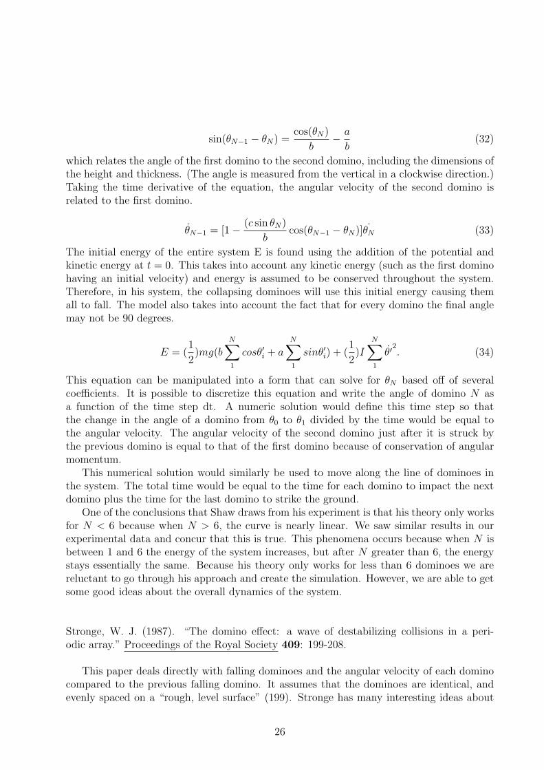
sin(θN−1 − θN) =cos(θN)

b− a

b(32)

which relates the angle of the first domino to the second domino, including the dimensions ofthe height and thickness. (The angle is measured from the vertical in a clockwise direction.)Taking the time derivative of the equation, the angular velocity of the second domino isrelated to the first domino.

θ̇N−1 = [1− (c sin θN)

bcos(θN−1 − θN)] ˙θN (33)

The initial energy of the entire system E is found using the addition of the potential andkinetic energy at t = 0. This takes into account any kinetic energy (such as the first dominohaving an initial velocity) and energy is assumed to be conserved throughout the system.Therefore, in his system, the collapsing dominoes will use this initial energy causing themall to fall. The model also takes into account the fact that for every domino the final anglemay not be 90 degrees.

E = (1

2)mg(b

N∑1

cosθ′i + a

N∑1

sinθ′i) + (1

2)I

N∑1

θ̇′2. (34)

This equation can be manipulated into a form that can solve for θN based off of severalcoefficients. It is possible to discretize this equation and write the angle of domino N asa function of the time step dt. A numeric solution would define this time step so thatthe change in the angle of a domino from θ0 to θ1 divided by the time would be equal tothe angular velocity. The angular velocity of the second domino just after it is struck bythe previous domino is equal to that of the first domino because of conservation of angularmomentum.

This numerical solution would similarly be used to move along the line of dominoes inthe system. The total time would be equal to the time for each domino to impact the nextdomino plus the time for the last domino to strike the ground.

One of the conclusions that Shaw draws from his experiment is that his theory only worksfor N < 6 because when N > 6, the curve is nearly linear. We saw similar results in ourexperimental data and concur that this is true. This phenomena occurs because when N isbetween 1 and 6 the energy of the system increases, but after N greater than 6, the energystays essentially the same. Because his theory only works for less than 6 dominoes we arereluctant to go through his approach and create the simulation. However, we are able to getsome good ideas about the overall dynamics of the system.

Stronge, W. J. (1987). “The domino effect: a wave of destabilizing collisions in a peri-odic array.” Proceedings of the Royal Society 409: 199-208.

This paper deals directly with falling dominoes and the angular velocity of each dominocompared to the previous falling domino. It assumes that the dominoes are identical, andevenly spaced on a “rough, level surface” (199). Stronge has many interesting ideas about

26

the modeling of falling dominoes. For example, he determines a ratio for the angular velocityat the beginning of one collision vs. the angular velocity at the beginning of the one beforeit. At the end of his paper, Stronge summarizes his five biggest conclusions:

1. There is a natural propagation speed for the collisions if the domino thickness is atleast half the distance between two dominoes.

2. As the number of dominoes that have fallen increase, the propagation speed shouldapproach this “intrinsic speed” (206).

3. For dominoes that are grouped closer together, momentum is not conserved fromcollision to collision.

4. If there is a lot of friction, a domino can reverse direction during a collision.5. While dominoes arranged farther from one another have only one collision at a time,

dominoes arranged closer together have multiple collisions, so that each new collision buildsupon the last.

This source is very useful right now as a complicated example of the factors we shouldtake into consideration when forming our initial model. It will be incredibly useful in thefuture when we are ready to consider a system that loses kinetic energy or a system where thedominoes slide or a system where a domino hits another domino and then reverses direction.

Stronge, W. J. and D. Shu (1988). “The domino effect: successive destabilization bycooperative neighbors.” Proceedings of the Royal Society 418 155-163.

This article assumes all of the conclusions proven in the previous article (see above).It does, however, take the model one step further. It analyzes an enormous row of fallendominoes, all leaning on the currently falling domino. It also neglects friction as well asthe coefficient of restitution. Instead of just having a ratio for successive angular velocities,Stronge and Shu calculate the ratio of the kinetic energy for the currently falling domino vs.the kinetic energy that the first domino had while it was falling. The most groundbreakingpart of this paper is the idea that when the distance between dominoes is large, “there aresome multiple collisions and some single collisions” (162). Also, when the distance betweendominoes is small and one domino falls on another, there is either “multiple collisions” orthe impact between dominoes is “sliding” (162). This really demonstrates to me how com-plicated it is to tell how fast linear, evenly spaced dominoes fall. Additionally, Stronge andShu experimentally test their theory to determine how accurate their model is. It is veryclever that they used small rectangular blocks as opposed to actual dominoes in all of theirexperiments, since dominoes tend to differ slightly in their dimensions. Also, although theirmodel assumed the coefficient of restitution was negligible, when in fact, it was measuredat at least one half in each experiment, their “cooperative group theory” model still veryclosely predicts their experimental data (161).

This article should be even more helpful in the future than the previous article. Althoughthe model is much more complex than the previous model, it is very accurate, and if we couldimprove it even a little, we would have a very good understanding of the time it takes linear,evenly spaced dominoes to fall.

27

Watts, D. J. (2002). “A simple model of global cascades on random networks.”Proceedings of the National Academy of Science 99(9): 5766-5771.

Watts studied the large cascades, called global cascades. An example of global cascadeis the cascading failure of power transmission grid in the western United States in August10, 1996. Global cascades seldom occur and are extremely difficult to predict. Networkinfrastructure is composed of nodes. It is found that the more traffic connected to thenode, the more likely it will trigger a cascade when compared to an average connected node.Moreover, initial failures also increase the probability of subsequent failures. The modelstudied in the journal was a model of motivation named “Binary decisions with externalities.”This model studied the decision made by an individual depend solely on the decisions ofothers in this model. The propagation of cascades is limited by the global connectivity ofthe network when the network of interpersonal influences is fairly sparse. Another behavioris when the network of interpersonal influences if fairly dense, the propagation of cascadesis limited by the stability of the individual nodes.

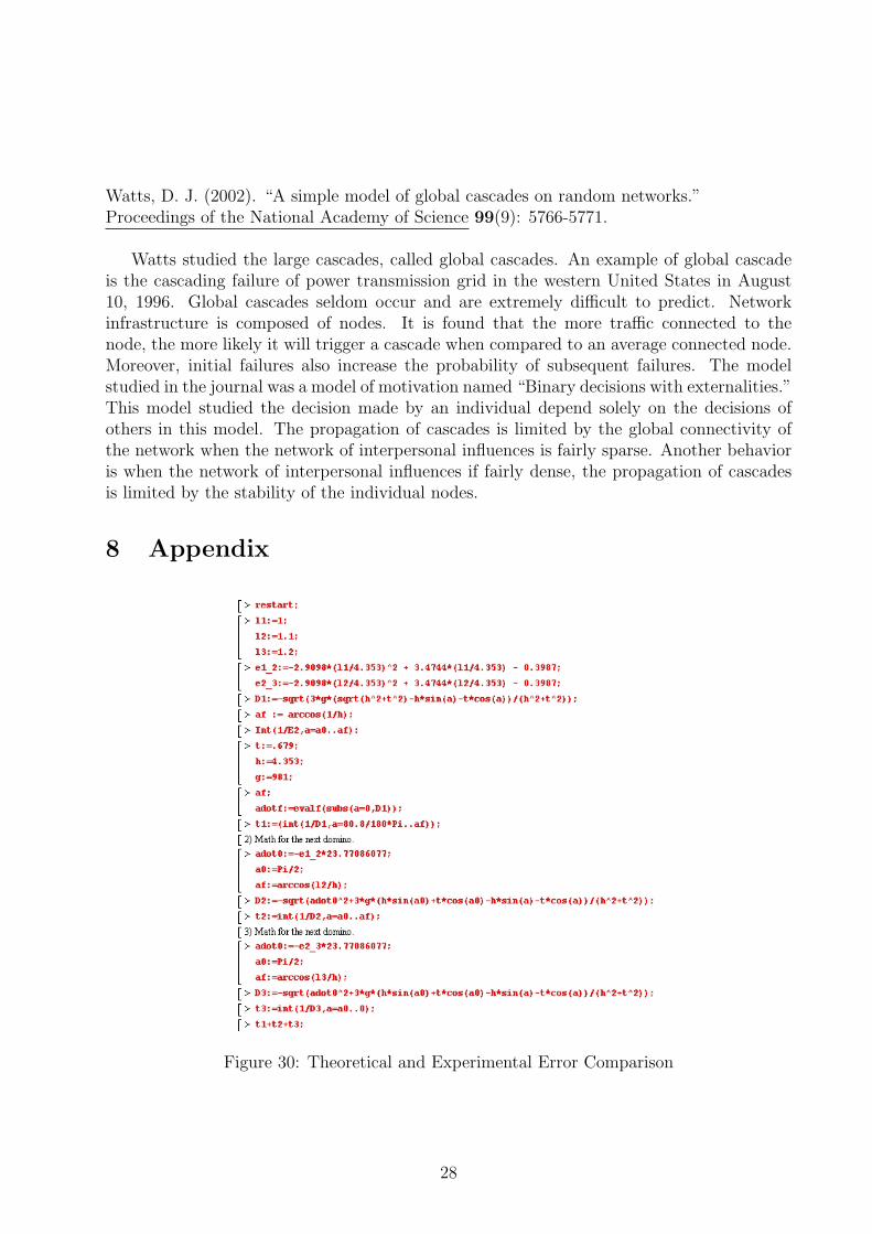
8 Appendix

Figure 30: Theoretical and Experimental Error Comparison

28