Fall, 2012 EMBA 512 Demand Forecasting Boise State University 1 Demand Forecasting.

Fall, 2012 EMBA 512 Demand ForecastingBoise State University

1

Demand Forecasting


2

Objectives• Understand the role of forecasting• Understand the issues• Understand basic tools and techniques


3

Forecasting• Developing predictions or estimates of

future values– Demand volume– Price levels– Lead times– Resource availability– ...


4

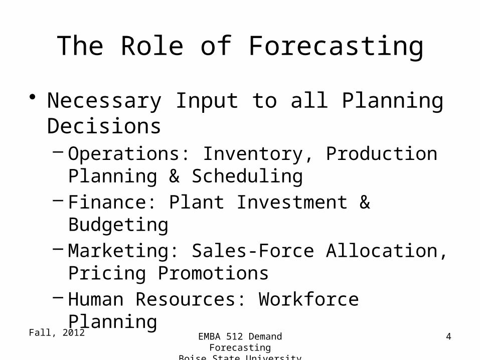
The Role of Forecasting

• Necessary Input to all Planning Decisions– Operations: Inventory, Production Planning &

Scheduling– Finance: Plant Investment & Budgeting– Marketing: Sales-Force Allocation, Pricing

Promotions– Human Resources: Workforce Planning


5

Demand Forecasting

For manufactured items and conventional goods, forecasts are used to determine

• Replenishment levels and safety stocks• Set production plans• Determine procurement schedules• Capacity planning, financial planning, &

workforce planning


6

Demand Forecasting

For services, demand forecasts are used for• Capacity planning, workforce scheduling,

procurement & budgeting.• Because services cannot be stored,

demand forecasting for services is often concerned with forecasting the peak demand, rather than the average demand and its range.


7

Characteristics of Forecasts

• Forecast are always wrong. A good forecast is more than a single value.

• Forecast accuracy decreases with the forecast horizon.

• Aggregate forecasts are more accurate than disaggregated forecasts.


8

Independent vs. Dependent Demand

• Independent– Exogenously controlled– Subject to random or unpredictable changes– What we forecast

• Dependent or Derived– Calculated or derived from other sources– Do not forecast


9

Forecasting MethodsQualitative or Judgmental

– Ask people who ought to know• Historical Projection or Extrapolation

– Time Series Models• Moving Averages• Exponential Smoothing

– Regression based methods


10

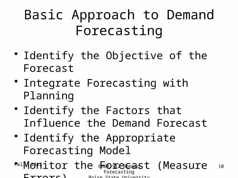
Basic Approach to Demand Forecasting

• Identify the Objective of the Forecast• Integrate Forecasting with Planning• Identify the Factors that Influence the

Demand Forecast• Identify the Appropriate Forecasting Model• Monitor the Forecast (Measure Errors)


11

Time Series Methods

• Appropriate when future demand is expected to follow past demand patterns.

• Future demand is assumed to be influenced by the current demand, as well as historical growth and seasonal patterns.


12

Time Series Models

With time series models observed demand can be broken down into two components: systematic and random.

Observed Demand = Systematic Component + Random Component


13

Time Series Methods

The systematic component is the expected demand value. It is comprised of the underlying average demand, the trend in demand, and the seasonal fluctuations (seasonality) in demand.


14

Idea Behind Time Series Models

Distinguish between random fluctuations and true changes in

underlying demand patterns.


15

Time Series Components of Demand

Time

Demand

Random component

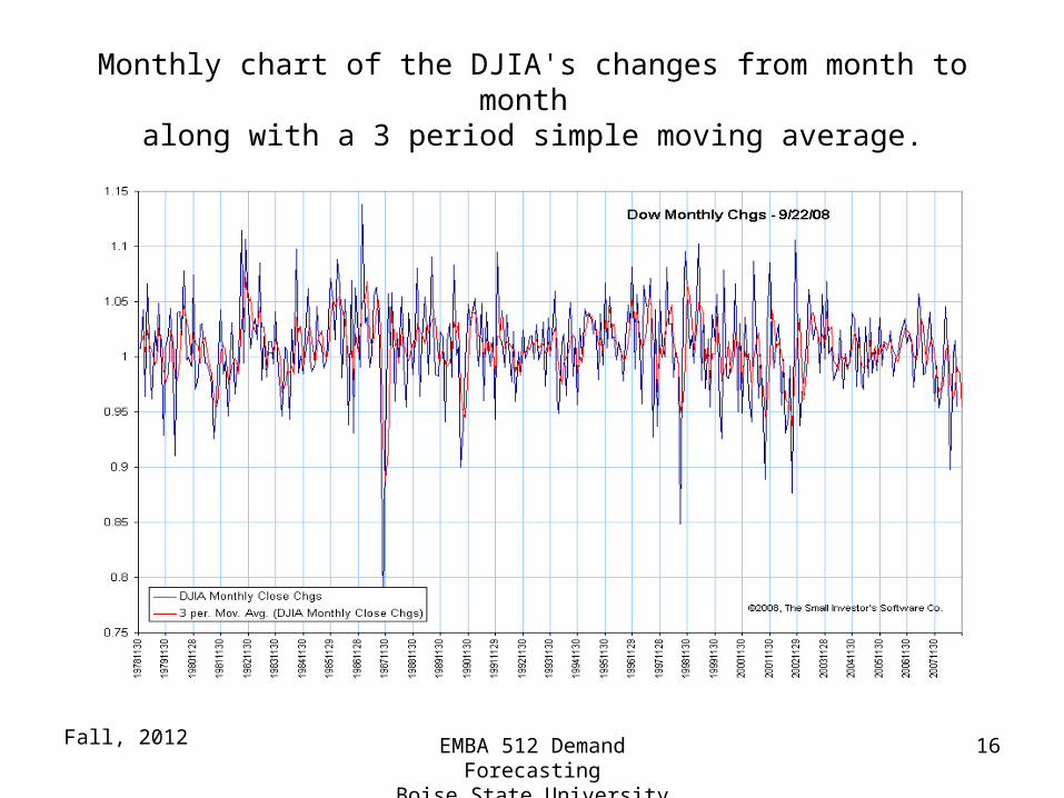
Monthly chart of the DJIA's changes from month to month along with a 3 period simple moving average.

Fall, 2012 16EMBA 512 Demand ForecastingBoise State University


17

Time Series Methods

• The random component cannot be predicted. However, its size and variability can be estimated to provide a measure of forecast error. The objective of forecasting is to filter the random component and model (estimate) the systematic component.


18

Moving Averages• Simple, widely used• Reduce random noise• One Extreme

– Prediction next period = Demand this period• Another Extreme

– Prediction next period = Long run average• Intermediate View

– Prediction next period = Average of last n periods


19

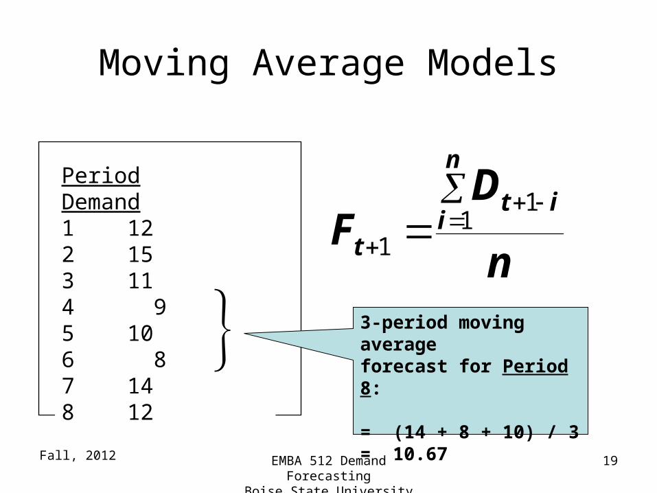
Moving Average Models

Period Demand1 122 153 114 95 106 87 148 12

3-period moving averageforecast for Period 8:

= (14 + 8 + 10) / 3= 10.67

n

DF

n

iit

t

11

1


20

Weighted Moving Averages

Forecast for Period 8= [(0.5 14) + (0.3 8) + (0.2 10)] / (0.5 + 0.3 + 0.2)= 11.4

What are the advantages?What do the weights add up to?Could we use different weights?Compare with a simple 3-period moving average.

n

iit

n

iitit

tW

DWF

11

111

1


21

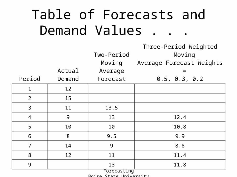
Table of Forecasts and Demand Values . . .

PeriodActual

Demand

Two-PeriodMovingAverageForecast

Three-Period Weighted MovingAverage Forecast Weights =

0.5, 0.3, 0.2

1 12

2 15

3 11 13.5

4 9 13 12.4

5 10 10 10.8

6 8 9.5 9.9

7 14 9 8.8

8 12 11 11.4

9 13 11.8


22

. . . and Resulting Graph

Note how the forecasts smooth out variations

0

5

10

15

20

1 2 3 4 5 6 7 8 9

Period

Volu

me Demand

2-Period Avg

3-Period Wt. Avg.


23

Simple Exponential Smoothing

• Sophisticated weighted averaging model• Needs only three numbers:

Ft = Forecast for the current period tDt = Actual demand for the current period t

a = Weight between 0 and 1


24

Exponential Smoothing

• Moving Averages – Equal weight to older observations

• Exponential Smoothing– More weight to more recent observations

• Forecast for next period is a weighted average of – Observation for this period– Forecast for this period


25

Simple Exponential Smoothing

Formula

Ft+1 = Ft + a (Dt – Ft) = a × Dt + (1 – a)

× Ft

• Where did the current forecast come from?• What happens as a gets closer to 0 or 1?• Where does the very first forecast come from?


26

Exponential Smoothing Forecast with a = 0.3

F2 = 0.3×12 + 0.7×11 = 3.6 + 7.7 = 11.3

F3 = 0.3×15 + 0.7×11.3 = 12.41

PeriodActual

Demand

Exponential Smoothing Forecast

1 12 11.00 (given)

2 15 11.30

3 11 12.41

4 9 11.99

5 10 11.09

6 8 10.76

7 14 9.93

8 12 11.15

9 11.41


27

Resulting Graph

0

2

4

6

8

10

12

14

16

1 2 3 4 5 6 7 8 9

Period

De

ma

nd

Demand

Forecast


28

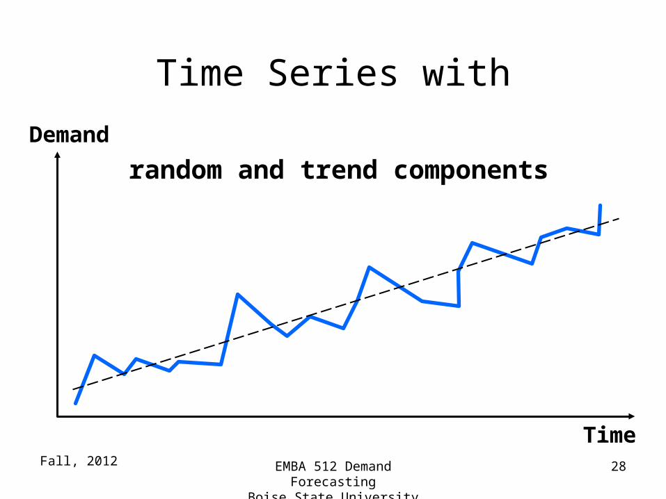
Time Series with

Time

Demand

random and trend components


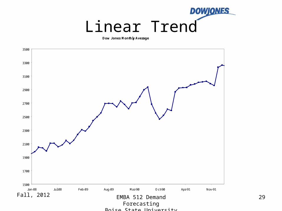
29

Linear TrendDow Jones Monthly Average

1500

1700

1900

2100

2300

2500

2700

2900

3100

3300

3500

Jan-88 Jul-88 Feb-89 Aug-89 Mar-90 Oct-90 Apr-91 Nov-91


30

Exponential TrendIntel Quarterly Sales in Millions of Dollars

$0

$500

$1,000

$1,500

$2,000

$2,500

$3,000

$3,500

$4,000

$4,500

$5,000

12/19/85 5/3/87 9/14/88 1/27/90 6/11/91 10/23/92 3/7/94 7/20/95


31

Trends

What do you think will happen to a moving average or exponential smoothing model

when there is a trend in the data?


32

Simple Exponential Smoothing Always Lags A Trend

Because the modelis based onhistorical demand,it always lagsthe obviousupward trend

PeriodActual

Demand

Exponential Smoothing Forecast

1 11 11.00

2 12 11.00

3 13 11.30

4 14 11.81

5 15 12.47

6 16 13.23

7 17 14.06

8 18 14.94

9 15.86


33

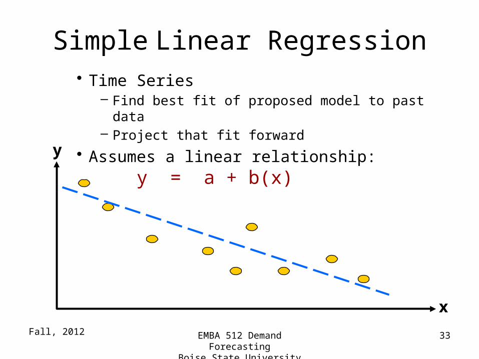
Simple Linear Regression• Time Series

– Find best fit of proposed model to past data– Project that fit forward

• Assumes a linear relationship: y = a + b(x)

y

x


34

Definitions

Y = a + b(X)

Y = predicted variable (i.e., demand)

X = predictor variable

“X” is the time period for linear trend models.


35

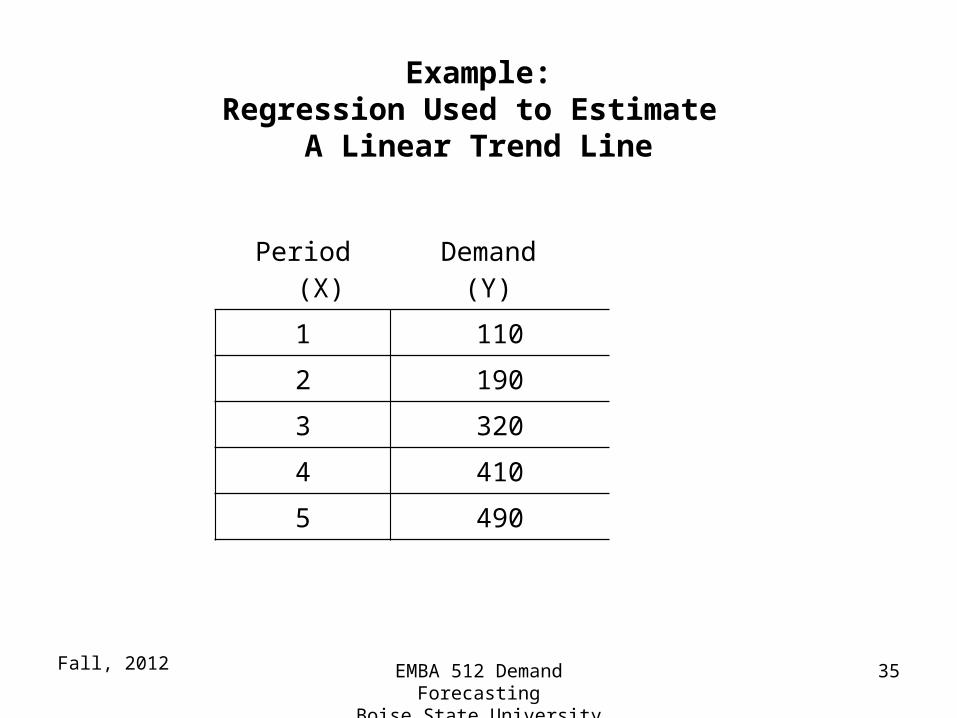
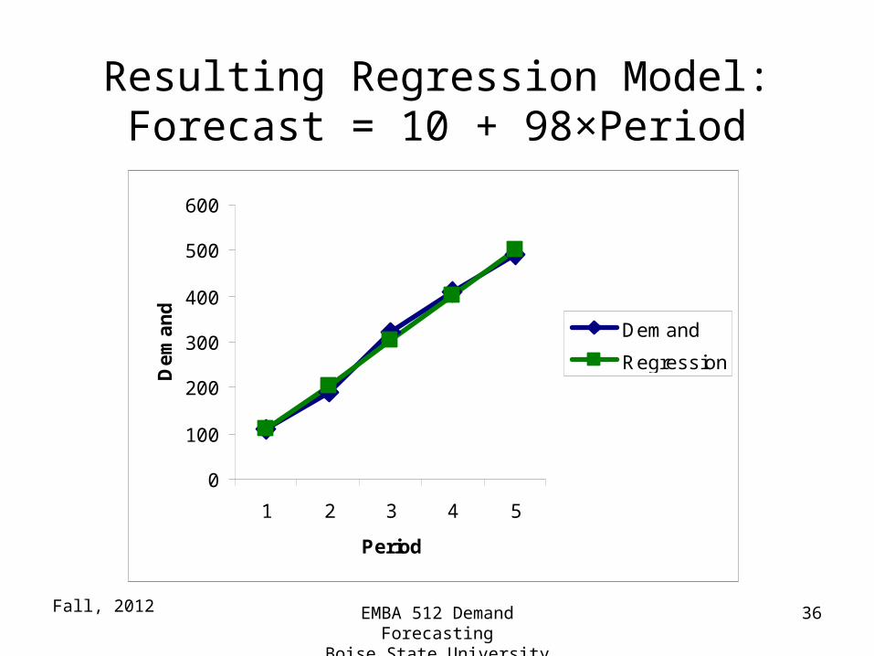
Example:Regression Used to Estimate

A Linear Trend Line

Period (X)Demand

(Y)

1 110

2 190

3 320

4 410

5 490


36

Resulting Regression Model:Forecast = 10 + 98×Period

0

100

200

300

400

500

600

1 2 3 4 5

Period

De

ma

nd

Demand

Regression


37

Time series with

Demand

random, trend and seasonal components

June June June June


38

Trend & SeasonalityCoca Cola Quarterly Sales in Millions of Dollars

$1,000

$1,500

$2,000

$2,500

$3,000

$3,500

$4,000

$4,500

$5,000

$5,500


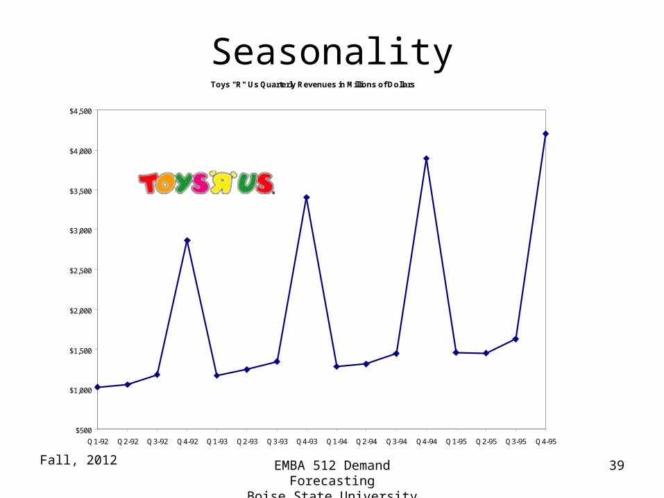
39

SeasonalityToys "R" Us Quarterly Revenues in Millions of Dollars

$500

$1,000

$1,500

$2,000

$2,500

$3,000

$3,500

$4,000

$4,500

Q1-92 Q2-92 Q3-92 Q4-92 Q1-93 Q2-93 Q3-93 Q4-93 Q1-94 Q2-94 Q3-94 Q4-94 Q1-95 Q2-95 Q3-95 Q4-95


40

Modeling Trend & Seasonal Components

Quarter Period Demand

Winter 07 1 80Spring 2 240Summer 3 300Fall 4 440Winter 08 5 400Spring 6 720Summer 7 700Fall 8 880


41

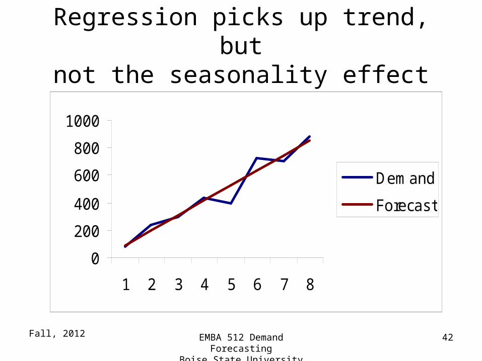
What Do You Notice?

Forecasted Demand = –18.57 + 108.57 x Period

PeriodActual

DemandRegression

ForecastForecast

ErrorWinter 07 1 80 90 -10

Spring 2 240 198.6 41.4Summer 3 300 307.1 -7.1

Fall 4 440 415.7 24.3Winter 08 5 400 524.3 -124.3

Spring 6 720 632.9 87.2Summer 7 700 741.4 -41.4

Fall 8 880 850 30


42

Regression picks up trend, butnot the seasonality effect

0

200

400

600

800

1000

1 2 3 4 5 6 7 8

Demand

Forecast


43

Calculating Seasonal Index: Winter Quarter

(Actual / Forecast) for Winter Quarters:

Winter ‘07: (80 / 90) = 0.89Winter ‘08: (400 / 524.3) = 0.76

Average of these two = 0.83

Interpret!


44

Seasonally Adjusted Forecast Model

For Winter Quarter

[ –18.57 + 108.57×Period ] × 0.83

Or more generally:

[ –18.57 + 108.57 × Period ] × Seasonal Index


45

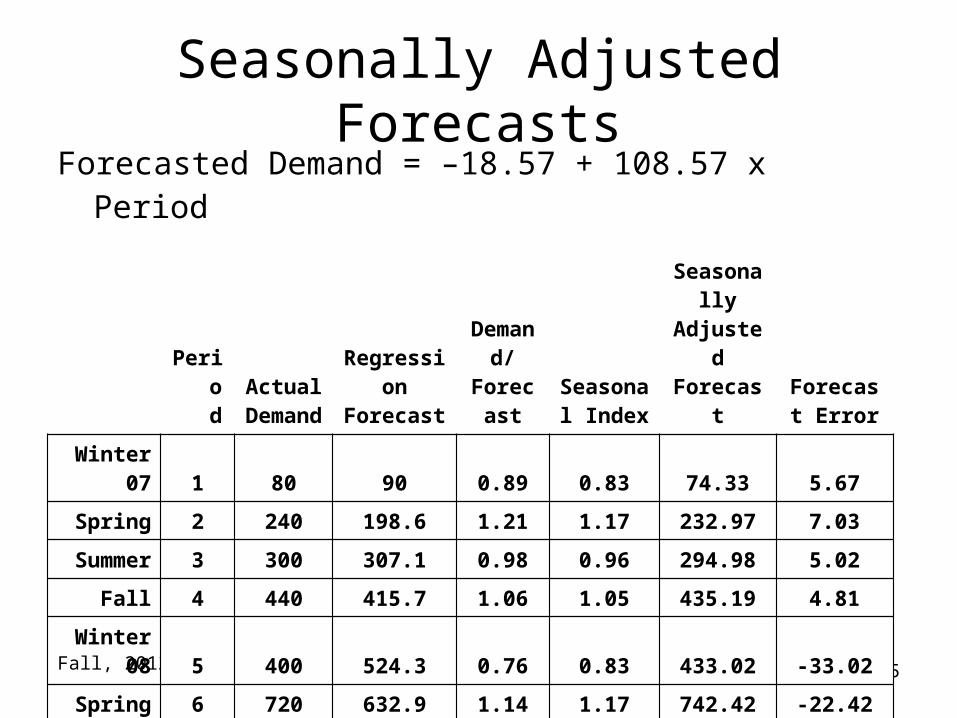
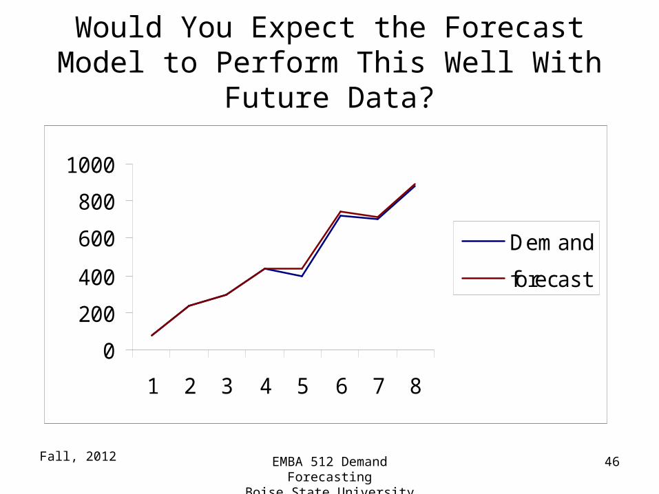
Seasonally Adjusted Forecasts

Forecasted Demand = –18.57 + 108.57 x Period

PeriodActual

DemandRegression

ForecastDemand/Forecast

Seasonal Index

Seasonally Adjusted Forecast

Forecast Error

Winter 07 1 80 90 0.89 0.83 74.33 5.67

Spring 2 240 198.6 1.21 1.17 232.97 7.03

Summer 3 300 307.1 0.98 0.96 294.98 5.02

Fall 4 440 415.7 1.06 1.05 435.19 4.81

Winter 08 5 400 524.3 0.76 0.83 433.02 -33.02

Spring 6 720 632.9 1.14 1.17 742.42 -22.42

Summer 7 700 741.4 0.94 0.96 712.13 -12.13

Fall 8 880 850 1.04 1.05 889.84 -9.84


46

Would You Expect the Forecast Model to Perform This Well With Future Data?

0

200

400

600

800

1000

1 2 3 4 5 6 7 8

Demand

forecast


47

The Perfect (Imaginary) Forecast

Actual vs. Forecast

0

200

400

600

800

1000

1200

1400

0 200 400 600 800 1000 1200 1400

Actual Demand

Fore

cast

Dem

and


48

A More Realistic Forecast

Actual vs. Forecast

0

100

200

300

400

500

600

700

800

900

1000

1100

1200

1300

1400

0 100 200 300 400 500 600 700 800 900 1000 1100 1200 1300 1400

Actual Demand

Fo

reca

st D

eman

d


49

Forecast Error• Building a Forecast

– Fit to historical data– Project future data

• Forecast Error– How well does model fit historical data– Do we need to tune or refine the model– Can we offer confidence intervals about our

predictions


50

Forecast Error

• The forecast error measures the difference between the actual demand and the forecast of demand. The forecast is based on the systematic component and the random component is estimated based on the forecast error.

• Forecast Error = Actual – Forecast


51

Measures of Forecast Accuracy

• Forecast Errort (Et)= Demandt-Forecastt

• Mean Squared Error (MSE) • Mean Absolute Deviation (MAD)• Bias • Tracking Signal • Relative Forecast Errors


52

Mean Squared Error (MSE)

n

tt

n EnMSE

1

21

The MSE estimates the variance of the forecast error.


53

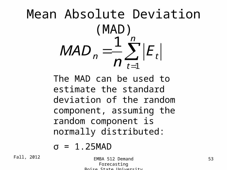
Mean Absolute Deviation (MAD)

n

ttn E

nMAD

1

1

The MAD can be used to estimate the standard deviation of the random component, assuming the random component is normally distributed:

σ = 1.25MAD


54

Bias

• To determine whether a forecasting method consistently over-or- underestimates demand, calculate the sum of the forecast errors:

n

ttn EBias

1


55

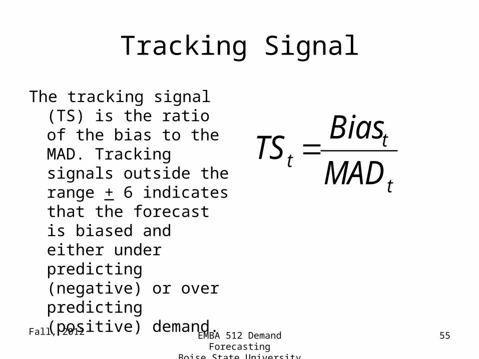
Tracking Signal

The tracking signal (TS) is the ratio of the bias to the MAD. Tracking signals outside the range + 6 indicates that the forecast is biased and either under predicting (negative) or over predicting (positive) demand.

t

tt MAD

BiasTS


56

Forecast Accuracy & Demand Variability (Normally Distributed Demand)

Coefficient of Variation

Probability Demand is Within

25% of the Forecast

0.10 98.76%

0.25 68.27%

0.50 38.29%

0.75 26.11%

1.00 19.74%

1.50 13.24%

2.00 9.95%

3.00 6.64%


57

• Forecasting is a necessary evil, try to reduce the need for it.

• Complexity costs money, does it provide better forecasts?

• Aggregation provides accuracy, but precludes local information

• Forecast the right thing

Issues


58

Forecasting Success Story

Taco Bell


59

Taco Bell• Labor is 30% of revenue• Make to order environment• Significant “seasonality”

– 52% of days sales during lunch – 25% of days sales during busiest hour

• Balance staff with demand

Feed the dog


60

Value Meals• Drove demand

• Forecasting system in each store– forecasts arrivals within 15 minute intervals

• Simulation system – “predicts” congestion and lost sales

• Optimization system– Finds the minimum cost allocation of workers


61

Forecasting System• Customer arrivals by 15-minute interval of

day (e.g., 11:15-11:30 am Friday)• Fed by in-store computer system• 6-week moving average• Estimated savings: Over $40 Million in 3

years.

Fall, 2012 EMBA 512 Demand Forecasting Boise State University 1 Demand Forecasting.

Documents

Transcript of Fall, 2012 EMBA 512 Demand Forecasting Boise State University 1 Demand Forecasting.