Fakultet for ingeniørvitenskap - IV - NTNU
47
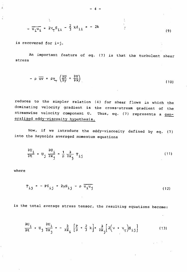
" -. ,. INTRODUCTION TO TURBULENCE MODELLING by Helge I. Andersson Lecture Notes in Subject 76572 Turbulent Flow Division of Applied Mechanics Department of Physics and Mathematics Norwegian Institute of Technology Trondheim, October 1988 TABLE OF CONTENTS page 1. Introduction 1 2. The generalized eddy-viscosity concept 2 3. .rurbulent conductivity 5 4. Zero-equation models 7 4.1 Constant eddy-viscosity models 9 4.2 Mixing-length models 10 4.3 Characterizing features 14 5. One-equation models 17 5.1 Transport equation for k 19 5.2 Transport equation for the eddy viscosity 25 5.3 Transport equation for the shear stress 25 5.4 Characteristic features 27 6. Two-equation models 29 6.1 The k-~ model of turbulence 30 6.2 Numerical examples 33 6. 3 ~_dvantages and disadvantages 40 7. Reynolds stress models 42 References for supplementary reading 46
Transcript of Fakultet for ingeniørvitenskap - IV - NTNU

~~
"
-. ,.
INTRODUCTION TO
TURBULENCE MODELLING
by
Helge I. Andersson
Lecture Notes in Subject 76572 Turbulent FlowDivision of Applied Mechanics
Department of Physics and MathematicsNorwegian Institute of Technology
Trondheim, October 1988
TABLE OF CONTENTS page
1. Introduction 1
2. The generalized eddy-viscosity concept 2
3. .rurbulent conductivity 5
4. Zero-equation models 7
4.1 Constant eddy-viscosity models 94.2 Mixing-length models 104.3 Characterizing features 14
5. One-equation models 17
5.1 Transport equation for k 195.2 Transport equation for the eddy viscosity 255.3 Transport equation for the shear stress 255.4 Characteristic features 27
6. Two-equation models 29
6.1 The k-~ model of turbulence 306.2 Numerical examples 336. 3 ~_dvantages and disadvantages 40
7. Reynolds stress models 42 .'
:
References for supplementary reading 46 :,~i

;;
- 1 -
1. INTRODUCTION
It is generally accepted that turbulent flows are exactly "
represented by three-dimensional time-dependent Navier-Stokes equ-
ations, which are the second-order Chapman-Enskog approximation
to the Boltzmann equation for molecular motion. Althoug existing
computer algorithms arid programs are capable of solving the full
Navier-Stokes equations, the storage capacity of present day compu-
ters is too small to allow the resolution of the tiniest small-
scale fluctuations of the turbulence.
Most flows of engineering importance are turbulent, and the
desire to make practical calculations useful in design and planning
has led to the development of approximate methods which make computer
simulations of turbulent flows feasible. The first step towards
fairly general prediction methods is the Reynolds-averaging of
the governing conservation equations. However, while the process
of carefully averaging the momentum and thermal-energy equations
can be considered an exact procedure, the resulting averaged equ-
ations do not contain enough information about the turbulence to
form a soluble set of equations. For example, unknown averages
of products of fluctuating quantities:
T.. = - P ~ (1)1J 1 J
QJ. = pc u-:--e (2)P J
appear in the Reynolds averaged momentum and thermal-energy equation,
respectively. Here, eq. (1) represents the apparent turbulent
stresses (Reynolds' stresses), while eq. (2) represents an apparent
turbulent heat conduction in the j'th direction. It should be
remembered, however, that the turbulent stresses and heat flux
account for the physical mechanisms of turbulent transport (convec-
tion) of momentum and heat, respectively.
The process of replacing the unknown averages of products
of fluctuating quantities with equations for (or functions of)
variables which can be considered as dependent variables in the
problem is called modelling. For instance, an equation that suppos-
edly expresses a relation between the unknown Reynolds stresses(1) and the mean velocity components is a turbulence model.

- - 2 -
A turbulence model can be either an algebraic relation or
a set of transport equations for some characteristic turbulent
quantities. The various models are often classified according
to the number of extra partial differential equations which are
considered in addition to the Reynolds-averaged Navier-Stokes equ-
ations. By selecting a proper turbulence model, the total number
of equations involved equals the number of unknown variables, and
a closed set of governing equations is obtained.
The objective of these lecture notes is to outline the essen-
tial ingredients involved in modern turbulence modelling, and to
demonstrate the effectiveness and capabilities of some representative
models at each level (according to the above classification scheme).
We are focussing on the various models required for the solution
of the Reynolds averaged momentum equation, from which the basic
ideas and principles are illuminated. The modelling required for
the solution of the thermal-energy equation follows basically the
same philosophy and strategy. Thus, only a brief account on the
modelling of the turbulent heat flux is given in section 3.
2. THE GENERALIZED EDDY-VISCOSITY CONCEPT
The convenience of the eddy-viscosity concept is coupled
with the mathematical convenience of retaining the same form of
the governing equations for laminar and turbulent flow, and there-
by allowing for the use of the same solution procedure in both
cases. Considering, for instance, the free shear flows like the
turbulent jet, wake and mixing-layer, the averaged streamwise moment-
um equation become: i..
i
"
u ~ + V ~ = - a~ (uv) (3) ~,
The orginal idea of Boussinesq was to define a turbulent or eddy-
viscosity by the relation
- au- PUV = pvT ay (4)

:r;:,~;;;i;:;;i~*;,?~:i;
- 3 -
If we substitute eq. (4) into eq. (3), the momentum equation become'
au au a ( au)u ax + V ay =ay vT -ay (5)
The eddy-viscosity defined by eq. (4) is not a physical property
like the molecular viscosity, but varies with local flow condi-
tions and the geometry of the problem. If the eddy-viscosity is
assumed to be constant, as suggested by Boussinesq in 1877, equ-
ation (5) becomes mathematically equivalent with the streamwise
momentum equations for the corresponding laminar free shear flows.
The value of the eddy viscosity, which can be obtained from experi-
ments, will generally be significantly greater than the molecular
viscosity.
For the free shear flows, only one of the Reynolds stresses
(1) appear in the momentum equation (3). In the general case,
however, relations like eq. (4) are required for all nine compo-
nents of the Reynolds stresses. In analogy with the molecular
stresses
cri j = 2 1.1 5 i j ( 6 )
the turbulent stresses can be modelled according to
T" = - p~ = 2pv 51.' )' - -32pko 1.' )' it.". (7)1.) 1. ) -r ,-~,
~~'\Here, the symbol k denotes the~kinetic energy of the turbulent
motion, defined as
k =: , ~ (8)1. 1.
which is a measure of the normal Reynolds stresses. The latter
term in the model (7) has been included to assure that the iden-
tity
: - 4 -
. ."- 2 ko = - 2k ,- uiui = 2\),Sii -"3 ii ' (9)
is recovered for i=j.
An important feature of eq. (7) is that the turbulent shear
stress
- ( aU av )- p uv = P\)! ay + ~ (10)
reduces to the simpler relation (4) for shear flows in which the
dominating velocity gradient is the cross-stream gradient of thestreamwise velocity component u. Thus, eq. (7) represents a gen-
eralized eddy-viscosity hypothesis.
Now, if we introduce the eddy-viscosity defined by eq. (7)into the Reynolds averaged momentum equations
aui aui 1 a- + u - = - - T (11)at j ax. pax. ij
) )
where
T.. = - Po.. + 2~S.. - p u-:-i::i-:-(12)1.) 1.). 1.) 1. )
is the total average stress tensor, the resulting equations become:
au. aui a [ p 2 ] a [ ( ) 1 -.:!::. + u. - = - '\- - + _3 k + '\- 2 \) + \) 5.. J (13) at J ax. ox. Pox. ,1.J) 1. J

- 5 -
"
These fundamental equations reveal~ that the effective viscosity
is the sum of the molecular and turbulent (eddy) viscosities. Fur-'
thermore, the turbulent kinetic energy k is the turbulent equivalent
to the averaged static pressure. Thus, if the kinetic energy is
not treated as a dependent variable of the model equations, k is
conveniently absorbed in the unknown kinematic pressure.
3. TURBULENT CONDUCTIVITY
Following the idea behind the eddy viscosity concept, the
turbulent heat flux (2) is related to the gradient of the mean
temperature field according to
- ae- pcp Uj6 = KT"a"'Xj (14)
where Kt is the turbulent conductivity (or, alternatively, the eddy
conductivity). This relation is analogous to Fourier's law for
heat flux due to molecular agitation.
Now, if the assumption (14) is introduced in the averaged
thermal energy equation
[ ae ae ) - - - 2.9-Pc - + U. -;;-- - ~<t> ax. (15)p at J OXj J
where
ae -Q : - K- + pc u.e (16)
ax. p JJ
denotes the total mean heat flux, the resulting equation becomes

~-~- ~-~ ~~
...~ , - 6 -
! \.
j
[ ae ae ] - a[ ( ) ae ]pcp a-t + U j ax; = ~<I> - axj - \ K + ~ ~ (17)
This equation demonstrates that the turbulent conductivity adds
to the molecular conductivity to enhance the total heat fluxes.
In analogy with the thermal diffusivity caused by molecular
action, it may often be convenient to introduce the turbulent or
eddy diffusivity:
YT :: KT/pcp (18)
for the turbulent heat transfer. It should be emphasized, however,
that the turbulent diffusivity as well as the turbulent conductivity
are not fluid properties but depend on the mean flow and the turbu-
lence. These scalar quantities may therefore vary significantly
from point to point within a flow field.
The eddy-diffusivity hypothesis (14) is analogous to the
eddy-viscosity hypothesis (4), i.e. the turbulent transport of
a certain property is related to the gradient of that property.
Thus, eq. (14) is based on the assumption that the turbulent tran-
sport of heat is provided by similar processes as the turbulent
transport of momentum. The ratio of the respective coefficients
of diffusion is defined as the turbulent Prandtl number:
'0" = \) /Y (19)T T T
In spite of the fact that the eddy viscosity and the eddy diffu-
sivity may vary considerably throughout a flow field, it is experi-mentally verified that the ratio (19) is approximately constant
within a flow. Furthermore, the maguitude of the turbulent Prandtlnumber is approximately constant for a wide range a flow situations.

1
- 7 - -
This is the famous Reynolds analogy from 1874. Today, engi- .
nee ring heat and fluid flow calculations take advantage of this
analogy and take the turbulent Prandtl number to be a constant
close to 1.
4. ZERO-EQUATION MODELS
Turbulence models using only partial differential equations
for the mean velocity field, and no differential equation for the
turbulence are classified as zero-equation models. All models
belonging to this class use the generalized eddy-viscosity concept
(7). The eddy-viscosity is furthermore related to the mean flow
field via an algebraic relation. Therefore, these models are also
called algebraic models. Because of their simplicity, zero-equ-
ation models have received considerable interest over the years,
and have been in common use for sophisticated engineering appli-
cations during the past decades.
The very simplest approximation of the turbulent effects
on the mean flow can be achieved by assuming that the eddy-visco-
sity is proportional to the molecular viscosity, i.e.
vT = f . v (20)
throughout the flow field. The dimensionless constant f is typi-
cally of the order 1000. From a numerical point of view, this
approach does not require any modifications of computer codes des-
ignated for laminar flow calculations. The only implication of
the turbulence is the increased effective diffusivity, which in
general quenches numerical instabilities arising from diffusion-
like truncation errors.
It is interesting to notice that some useful information
about the flow field may be obtained by this simple approach. For
instance, Hanson, Summers and Wilson (1984,1986) simulated the
wind flow over buildings numerically using the eddy-viscosity model
(20). Figure 1 a shows the predicted wind-flow environment for

~",~
"c - 8 - ..,
.
.; iji~; / I :: '::!.!:~~~~f~:.; 'Jl1
,/
./-;
Fig.l Predicted wind-flow environment for a two-building config-
uration in 3D. Hand h denote the heigths of the downstream and
upstream buildings, respectively. L is the distance of separation.
(Figures taken from Hanson, Summers and Wilson 1986).
a) Streakline pattern for a vertical plane one meter from the
plane of symmetry. L/H = 1.0 and H/h = 5.0.
.8
.7
00.6 0 0
-I-~ .5
0ttJ .4a-U')b .3Z 0- 0~ .2 L/H = .5
.1
.0 .5 1.0 1.5 2.0
W/H
b) Maximum predicted reverse vortex speed at ground level (2m
above the ground) for the case L/H = 0.5. The symbols denote
wind-tunnel measurements by Penwarden and Wise 1975.

-
- 9 -
,a two-building configuration. The recirculation of the flow
downstream of the taller building and the reverse-vortex formed
between the buildings are clearily observed. Figure lb shows the
predicted maximum reverse-vortex speed at the ground level compared
with wind-tunnel measurements.
It should be emphasized, however, that eq.(20) cannot give
satisfactory results in the immediate vicinity of solid boundaries,
simply because the turbulence quenches close to a wall. Then,
according to eq. (7), the eddy viscosity should vanish at the boun-
daries.
4.1 Constant eddy-viscosity models
An example of the constant eddy-viscosity models is the simple
relation
vT = K . ~(x) . Us(x) (21)
suggested by Prandtl in 1942 for free shear flows. While K is
a dimensionless constant, the length scale and velocity scale in
eq.(2l) may be functions of the longitudinal distance x. Accor-
dingly, the eddy-viscosity is allowed to vary in the streamwise
direction but is supposed to be constant over any cross section
of the flow. This is certainly a rough assumption, in particular
in the vicinity of the edges of the shear layers. Due to the inter-
mittent nature of the flow in these regions, a fixed point in space
will alternately be within and outside the turbulent domain. Never-
theless, reasonable results for free shear flows are obtained with
the model (21).
Figure 2 shows that the solution obtained with the model
(21) is in quite good agreement with experimental data for the
plane jet. Near the edge of the jet, however, the experimentalresults indicate a somewhat faster reduction- of the velocity than
obtained by the constant eddy-viscosity model.

~
- 10 -1.0 ~_.- --- -
Ii ~ T~rv:.. "" - Goerllrrl1942J
V (x y) IV! '~'"' I, s 1- ' --- Tollmlrn 119261
~ II . Co Irs I 19561
! Lawollhr.wakr!I I
05 ~ -. -- T--,-., I
I
IDJla: Ii 0 Retchardt (19421 "r' . Foerthmann (19361 \\\.
,L '"\~ ~ .'. ~ ~,".. ." '
'... ~-oL-L-- J ...0 0.5 1.0 1.5 2.0 25
C= ~((
Fig.2 Comparison of theoretical velocity profile with experimental
data for a plane turbulent jet. The solid line is based on the
constant eddy-viscosity model (21), while Tollmien used a mixing-
length type model (22). (Figure taken from White 1974).
It should be remembered that in the particular case of a
plane wake, the streamwise variation of the eddy viscosity (21)
vanishes, and the eddy viscosity becomes a constant througout the
wake.
4.2 Mixing-length models
In order to account for a cross-stream variation of the eddy-
viscosity, for instance in the vicinity of a wall or near the edge
of a jet, Prandtl suggested in 1925 that
2 \dU \vT = £. ay (22)
where 1 is the mixing-length.
The model (22) was orginally based on the mixing-length hypo-
thesis, in which it was assumed that the turbulent eddies interact
by collisions in the same way as the molecules in a gas. Thus,the mixing-length became the turbulent equivalent of the molecular

-
- 11 -
~ ,
mean free path. However, it is today generally accepted that this
physical equivalence is completely erroneous. The turbulent eddies
are not small compared to the width of the mean flow, and they
interact continuously rather than collide instantaneously.
Nevertheless, the model (22) has proved successful in several
flow situations. This is probably due to the observation that
the eddy-viscosity from dimensional argumentss should be propor-
tional to a length scale and a velocity scale. Now, by takingthe velocity scale which characterizes the larger eddies as the
cross-stream velocity gradient times the mixing-length, the formula
(22) is obtained. Equation (22) can thus be considered as the
definition of the mixing-length, like eq. (7) defines the eddy-viscosity. The success of these concepts is achieved because the
latter quantities are more easily correlated with experimental
data than are the Reynolds stresses themselves.
By adopting the mixing-length hypothesis (22), an empirical
model for the mixing-length rather than for the eddy-viscosity
must be selected. prandtl orginally suggested that the mixing-
length should be proportional to the distance from the wall. This
is a reasonable assumption in the inner part of a wall flow, but
outside the viscous sublayer.
In the outer part of the wall layer, Fig.3 shows that the
mixing-length becomes approximately constant. This behaviour sugg-
ests the model:
I ry y ~ YiR. -- alo Yi .5 y
where (23)
r = 0.40 ; al = 0.075

- 12 -
008
0.07
006
OO~PI!
004
0.03
0.02
0.01
00 0.1 0.2 03 04 O~ 06 07 08 0.9 10
rIa
Fig.3 Dimensionless mixing-length distribution across a turbulent
boundary layer at zero pressure gradient, according to data of
Klebanoff 1954. (Figure taken from Cebeci & Bradshaw 1977).
007
006
OO~
004'""T
~00)
, , ,,
002 "
001
00 01 02 03 04 05 06 07 08 09 10
y/8
Fig.4 Dimensionless eddy-viscosity distribution across a turbu-
lent boundary layer at zero pressure gradient, according to data
of Klebanoff 1954. (Figure taken from Cebeci & Bradshaw 1977).

~~i\~~;:~¥~"
- 13 -
are dimensionless constants in accordance with experimental obser-
vations. The position Yi is determined so that the inner region
model should match the outer region model by the requirement of
continuity in the mixing-length.
By analogy with laminar flow over an oscillating flat plate
(Stokes' second problem), the modified mixing-length formula
t = ry [1 - exP(-yu*/VA+)] (24)
was proposed by van Driest in 1956 for the inner region. The term
in the square brackets accounts for the damping effect of the thin
viscous sub layer close to the wall, so that the mixing-length out-
side the viscous shear layer is effectively modified near the wall.
In accordance with experimental results, the dimensionless para-meter A+ = 26. Thus, the term in the square brackets increases
from zero at the wall to about 0.63 at y+ = 26, and tends to 1
as the normal distance from the wall is further increased.
Today, the most popular eddy-viscosity model based on the
mixing-length concept is the two-layer model
vT = [ (ry) 2 [1 - :XP(-YU*/VA+)]2 . 1i¥1 y ~ Yi (25a)
a2 . UE . 0 Yi ~ Y (25b)
proposed by Cebeci and Smith in 1970. Here
UE = inviscid velocity external to boundary layer
*0 = boundary layer displacement thickness
a2 = 0.0168 = dimensionless parameter

- 14 -
The inner region model is obtained by combining van Driest's modi-
fied mixing-length formula (24) with Prandtl's model (22). The
outer region model, on the other hand, is a simple constant eddy-
viscosity model like (21). With a different choise for velocity
and length scale, the outer model (25b) can be replaced by
"T = 0.3 . u* . <5 (26)
where
u* = friction velocity
<5 : boundary layer thickness
a3 : 0.060 - 0.075 : dimensionless parameter
It can easily be verified that the inner-region expression
(25a) yields a linearly increasing eddy-viscosity in the logar-
ithmic region, which is in accordance with the experimental data
plotted in Fig.4. In the outer half of the boundary layer, however,
the eddy-viscosity is observed to decrease. This is obviously
due to the intermittent nature of the outermost part of wall boundary
layers. This behaviour is sometimes accounted for by a dimensionless
function which reduces from 1 to 0 as y goes from 0.5 IS to 1.0 <5
In order to account for the intermittency, the eddy-viscosity model
(25) should be multiplied with this function or intermittency factor.
4.3 Characterizing features
Several eddy-viscosity and mixing-length models have been
used over the years, and some of them still are. Empirical corr-
ections have been made to some of the models to account for the
effects of pressure gradient, low Reynolds number, wall suction
or injection, and curvature effects.
Some typical numerical solutions for boundary layer flows
obtained with the Cebeci & Smith model (25) are shown in Figures
5 and 6. While Fig. 5 shows results for a zero-pressure gradient
flow, the boundary layer in Fig. 6 is in a moderate positive pres-sure gradient. Results for the entrance-region turbulent flow

- 15 -I , ~
"" 5
4
C, . 10']
Z
110' 106 10' In" Int
R~.
Fig.5 Calculated variation of local sk'in-friction coefficientfor zero pressure gradient turbulent boundary layer. The solidline denotes numerical solution of Cebeci & Smith 1974 using a
two-layer model like eq. (25). The symbols denote experimental
data.1.0 = 6.92 ft
0.8
0.6
!!-Ue
0.4
0.2 Re
0R x 10-" A A Ae
C x 10] c,f
0 00 Z 4 6 8
x (ft)
00 1 2 J 4 5
y (in.)
Fig.6 Numerical results of Cebeci & Smith 1974 and experimental
data of Bradshaw & Ferriss 1965 for an equilibrium boundary layerin moderate adverse pressure gradient. The symbols denote the
experimental data, and the solid lines denote calculations using
a two-layer model like eq. (25).

.
- 16 -
..3 i . 9 i . 33 i. 57 i . 80.5I. 0 0
0.8
0
0.6
I:-ro
0.4
0.2
O~b 0'.11 ".0 I ~20',0 d,o '~O 1,2
u/u C.b U~8 1',0 1,20 0~6, 0',8 1:0 1~2
Fig.7 Comparison of calculated and experimental velocity profiles
in the entrance region of turbulent pipe flow. The symbols denote
the experimental data of Barbin & Jones 1963, and the solid lines
denote the numerical solutions of Cebeci & Chang 1977 using an
algebraic turbulence model.
i0.4 !
o.
0.2
Ap.
0.1
0 10 20 30 40 50 60 70 80 90
x
Fig.8 Comparison of calculated and experimental pressure dropin the entrance region of turbulent pipe flow. The symbols de-
note the experimental data of Barbin & Jones 1963, and the solid
line denote the numerical solution of Cebeci & Chang 1977 using
an algebraic turbulence model.
,
Ij
~

- 17-
in a pipe with uniform entry velocity are shown in Figs. 7 and
8.
The advantages of the algebraic models can be summarizedas follows:
* They produce good results for simpler shear flows (free
shear flows as well as external and inernal boundary lay-
ers).* They are easy to use (i.e. include in existing computer codes).
* The model parameters are fairly constant.
* They can provide starting values for iterative calculation
procedures.
The most important limitations of the algebraic models are
that: ,
* Self-preservation is assumed; i.e. the mean flow and the
turbulence should depend only on local conditions.* They produce inaccurate results for separating boundary layers.
* They are not capable of predicting the flow in recirculat
ing zones.
5. ONE - EQUATION MODELS
Later in this section it will be demonstrated that the
mixing-length models are implicitly based on the assumption
that the turbulence is in a state of local equilibrium. There-
fore, the mixing-length models, and other algebraic models,
are unable to account for the transport of characteristic
turbulence quantities.
For instance, in pipe flow the turbulence is produced
near the walls and diffused towards the axis. The mixing-length
model (22), neglecting this transport process, predicts zero
turbulence at the centerline (due to the vanishing mean velocity
I
i

- 18-.
gradient;. Nevertheless, reasonable results for the mean flow
can be obtained (Figures 7 and 8). The algebraic models further-
more neglect the convective transport of turbulence. Accord-
ingly, they are not capable of predicting the downstream decay
of turbulence generated by a grid.
In the present section, models which account for the
convective and diffusive transport of turbulence are considered.
While the zero-equation models considered in the preceding
section were represented by some algebraic expressions, the
one-equation models typically consist of ~ partial different-
ial equation like:
2! + u If- = DIFF + PROD - DISS (27)at j aXj
Here, f is a characteristic scalar property of the turbulence.
The left side of eq. (27) represents the rate of change of
f within a fluid element, while the terms on the right side
account for the various mechanisms which may contribute to
the change of f; i.e. diffusion, production and dissipation.
Equation (27) is thus a differential tran~port equation for
the fluid property f.
The thermal-energy equation for laminar flow of an in-
compressibel fluid
[ ae ae ] a2e pcp at + Uj ~ = K ~~ + ~~ (28)
J J J
is a well-knovn transport equation which exhibits essentially
the same form as equation (27). Like in the model equation
(27), the first term on the right represents diffusion (due
to molecular transport)' and the second term represents produ-
ction of internal energy or heat (due to viscous dissipation).
Notice that no dissipation term occurs in the energy equation
(28) .
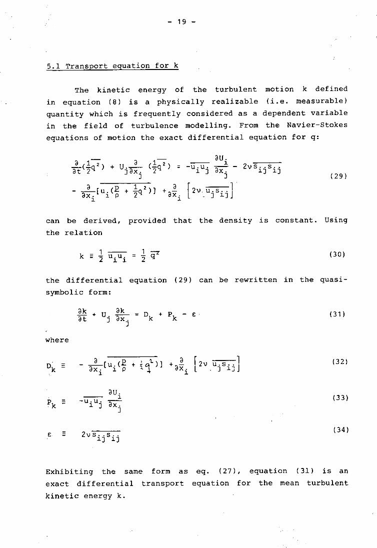
- 19 -
5.1 Transport equation for k
The kinetic energy of the turbulent motion k defined
in equation (8) is a physically realizable (i.e. measurable)
quantity which is frequently considered as a dependent variable
in the field of turbulence modelling. From the Navier-Stokes
equations of motion the exact differential equation for q:
- - aua ( 1 2 a ( 1 2 i
~ t -2q ) + u.~ -2q ) = -u.u. ~ - 2vs. .s..0 JoX. 1 J oX. 1J 1J
J J (29)a CE. 1 2 a r 1 .
- ~[u. + -2q )] +~- L 2V u.s. .JoXi 1 p oXi - J 1.J
can be derived, provided that the density is constant. Using
the relation
_1 1-=zk = "2 uiui = "2 q (30)
the differential equation (29) can be rewritten in the quasi-
symbolic form:
ak ak- + U. - = D + P - e: (31)at J ax. k k
J
where
Dk =: -;?- [ u . (E. + ~ '11. )] + ':I ~ rL 2 v u. s . . J' ( 32 )oXi 1 p .. J, oXi . J 1.J
au.P = -'U-:-u-: ~ (33)k - 1. J ox.
J
e: =: 2vs. .s.. (34)
1.J 1.J
Exhibiting the same form as eq. (27), equation (31) is an
exact differential transport equation for the mean turbulent
kinetic energy k.

~;~';['.!i~,: "~:":';"
- 20 -
Having established the additional equation (31), one
should not be led to the conclusion that the closure problem
(i.e. closing the set of equations) has been solved. Unfortu-nately, the terms (32) - (34) involve unknown correlations
of fluctuating quantities, and should therefore be subject
to some approximations (modelling).
The production ~ .Pk represents the production of
turbulent kinetic energy by work done by the interaction of
the mean flow and the turbulent stresses. It can easily be
demonstrated that Pk is positive under typical shear flow
conditions. It should also be remembered that the same term,:
but. with opposite sign, appears in the transport equation)
for the kinetic energy of the mean flow. Thus, Pk represents
the rate of energy transfer from the mean motion to the turbu-
lence.
Since the unknown Reynolds stresses are involved in
the production term, Pk kan be modelled by using the general-
ized eddy-viscosity hypothesis (7), i.e.
( 2 ) au. Pk = 2VT Sij - 3 °ij k ~)
(35)au. 2 au.
J. J.= 2vT S. . -;;-- - -3 k -;;--J.) ox. ox.
) J.
The mean flow is incompressible and the final model for the
production term becomes
au.- 2 J.Pk - vT Sij ax-:- (36)
)
This is an exact expression for the production term in terms
of the eddy-viscosity and the mean flow field.

- 21 -
The diffusive ~ Dk represents the diffusion of turbu-
lent kinetic energy due to turbulent and molecular transport.
Integrating the diffusive term over a volume which completely
encloses the turbulence, application of Gauss' theorem reveals
that the integral of Dk exactly vanishes. Accordingly, this
term neither creates nor destroys turbulent kinetic energy,
but merely promotes a spatial redistribution of it.
The diffusive transport due to molecular action, i.e.
the latter term in eq. (32), is negligible for high local
Reynolds numbers, and is therefore neglected (except in the
immediate vicinity of solid boundaries where viscous effects
always become significant). The turbulent contribution to
the transport of k is assumed to be analogous to the turbulent
transport of heat and momentum. Thus, in analogy with eq.(14),
we assume that
~-~?:---~2. E ::-T:; a k- u. ;; + + Rj - u. - q1Rj 'Y k ~ (37 )J. -- P J.1.t aX.
J.
where the proportionality factor is the turbulent diffusivity
of k. Following the Reynolds analogy between different tur-
bulent transport processes (Section 3), the diffusivity des-
cribing the turbulent transport of k is linearly related to
the eddy-diffusivity. Thus, the dimensionless diffusion number
\IT0=-k Yk (38)
should be (approximately) constant across a flow. Note the
analogy between eq. (38) and (19).
With equations (37) - (38), the modelled expression
for the diffusive term becomes:
a ( \IT ak )D = - - -- (39)k ax. Gk ax.
J. J.
where the dimensionless diffusion number should be determined
from experimental data.
~
..' .
- 22 -
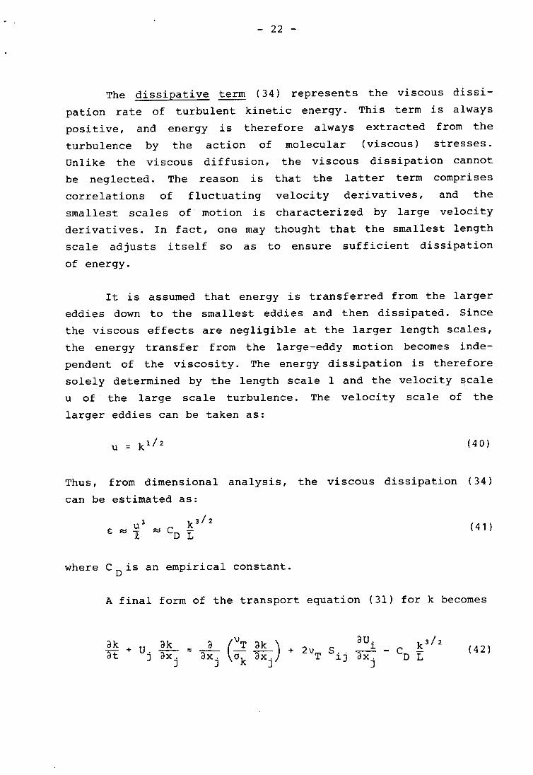
The dissipative ~ (34) represents the viscous dissi-
pation rate of turbulent kinetic energy. This term is always
positive, and energy is therefore always extracted from the
turbulence by the action of molecular (viscous) stresses.
Unlike the viscous diffusion, the viscous dissipation cannot
be neglected. The reason is that the latter term comprises
correlations of fluctuating velocity derivatives, and the
smallest scales of motion is characterized by large velocityderivatives. In fact, one may thought that the smallest length
scale adjusts itself so as to ensure sufficient dissipation
of energy.
It is assumed that energy is transferred from the larger
eddies down to the smallest eddies and then dissipated. Since
the viscous effects are negligible at the larger length scales,
the energy transfer from the large-eddy motion becomes inde-
pendent of the viscosity. The energy dissipation is therefore
solely determined by the length scale 1 and the velocity scale
u of the large scale turbulence. The velocity scale of the
larger eddies can be taken as:
u = k1/2 (40)
Thus, from dimensional analysis, the viscous dissipation (34)
can be estimated as:
U3 k3/2e:~_. ~C - (41)R. D L
where C D is an empirical constant.
A final form of the transport equation (31) for k becomes
~ + U ~ - a ( VT ak ) aui k3/2at j ax. - ~ Ok ax: + 2vT Sij ax-:- - CD L (42)
J J J J

- 23 - "
Here, the exact terms (32) - (34) have been replaced by the
modelled (approximate) terms (36), (39) and (41).The partial
differential equation (42) is a transport equation for the
turbulent kinetic energy (8). However, the use of the generali-
zed eddy viscosity hypothesis (7) introduces ~ unknown turbu-
lent quantities in the Reynolds averaged momentum equations:
the eddy viscosity and the turbulent kinetic energy. Therefore,
we have to establish a relation between these unknown quantities
which can used in connection with equation (42).
The first step in Prandtl's mixing-length hypotesis,
which ultimately led to eq. (22), is the assumption that the
eddy viscosity is proportional to a length scale and a velo-
city scale. An example of a model of this form is the simple
constant eddy-viscosity model (21) for free shear layers.
In his mixing-length approach Prandtl related the velocity
scale to the gradient of the mean velocity field. It can be
anticipated, however, that an improved expression for the
eddy viscosity is obtained if the velocity scale is taken
as a characteristic velocity for the turbulence rather than
for the mean flow.
Prandtl (in 1945) and Kolmogorov (in 1942) independ-
ently suggested that the velocity scale should be proportional
to the square root of the turbulent kinetic energy. Thus,
the Prandtl-Kolmogorov relation between the eddy-viscosity
and the turbulent kinetic energy becomes:
vT = c~ v'k L (43)
In this expression the eddy viscosity is related not only
to the mean flow, like in section 4, but it has also been
associated with the turbulence via k.
Now, the modelled transport equation (42) for k and
the relation (43) still involve the unspecified length scale
L. While k is obtained from the solution of the PDE (42),

--;-7 ;~,~~!:~~~
- 24 -
,
L is taken from an empirical algebraic expression. L, being
a meassure of the size of the larger turbulent eddies, can
be specified in a similar manner as the mixing-length in section
4.2. Thus, the accuracy of the complete model depends on the
quality of the selected expression for L.
The model equations (42), (43) furthermore involve three
dimensionless parameters, which should be determined from
available experimental information. In order to have a useful
turbulence model, it is required that these parameters are
approximately constant within a particular flow field, and
that they do not change from one flow situation to another.
Thus', it is desirable that the model parameters can be con-
sidered as being nearly universal constants.
Finally, in order to solve the PDE (42) boundary condi-
tions for k should be imposed. Outside a shear layer (a wall
boundary layer or a free shear layer) the turbulent kinetic
energy should vanish, i.e. k=O. At a line of symmetry (like
the axis in a pipe) the cross-stream variation of k should
vanish. Near solid boundaries the turbulent fluctuations are
damped so that k=O at the walls. However, we have neglected
the viscous part of the diffusion term (32), and the modelled
equation (42) cannot apply straight to the wall. Accordingly,
a condition on k is imposed at a certain position in the inner
part of the logarithmic region. The relevant value of k is
obtained by assuming that the production term is approximately
equal to the dissipation at this position. A detailed discussion
on boundary conditions for turbulent transport equations requi-
res some knowledge about computational fluid dynamics, and
is beyond the scope of this lectures.
In the case of thin shear layer flow a special case
of the k-equation (42) can be considered. In the near wall
region both the convective and diffusive transport of k are
negligible. Thus, the production term balances the dissipation.

I
- 25 - :
With this particular simplification the length scale L becomes: '.
L = £ (CD/C~) l/~ (44)
i.e. L is proportional to the mixing-length. This observation
demonstrates that the mixing-length models are applicable'
only when the turbulence is in a state of local equilibrium,
i.e. when the production and dissipation of turbulence energy
are in balance.
5.2 Transport equation for the eddy viscosity
A differential transport equation for the eddy viscosity
was proposed by Nee and Kovasznay in 1969. Like the k-mode1
(42), the Nee & Kovasznay model r<quires the specification
of a length scale via an emplrical expression.
Reasonable agreement with experimental results has been
obtained with the resulting model. Nevertheless, the model
has received only modest attention. This is probably because
its dependent variable is a non-physical quantity. While,
for instance, the mean turbulent kinetic energy and the Reynolds
stresses can be measured directly, the eddy-viscosity can
only be derived from experimental data via its "definition"
( 7 ) .
5.3 Transport equation for the shear stress
In 1967 Bradshaw, Ferriss and Atwell developed a one-
equation model which does not employ the generalized eddy
viscosity concept. While the eddy viscosity hypothesis (7)
relates the turbulent shear stresses to local mean flow condi-
tions only, the "structural" assumption

:;;;';;',ic;,:i::r;:~~:~~~~~
. . - 26 -
. '.
T.. = - p~ = apk ilj (45)1.J 1. J
relates the shear stresses to the turbulent kinetic energy
(i.e. the turbulent normal stresses). The assumption (45)
has been used earlier by Nevzglijadov (in 1945) and Dryden
(in 1948), and experimental investigations of wall boundary
layers suggest that the dimensionless constant a is approxi-
mately equal to 0.3.
The differential equation (31) with the right hand side
terms (32)-(34) is an exact transport equation for the mean
turbulent kinetic energy k. Bradshaw and his co-workers used
the "structural" assumption (45) and converted equation (31)into a transport equation for the dominating shear stress
component in wall boundary layers.
Since the shear Reynolds stress becomes a dependent
variable in this formulation, the production term should be
kept in its exact form (33), while the dissipative term (34)
is modelled according to the converted form of equation (41).
Bradshaw and co-workers did not employ the Reynolds analogy
for the diffusive term, but assumed that the diffusion of
the shear stress is proportional to a characteristic velocity
for the large eddies in the outer part of the wall boundary
layer.
The resulting model equation for the transport of the
shear stress involves two empirical functions. The dimension-
less "constant" a in the structural assumption (45) may also
be considered a function of the distance from the wall.
The Bradshaw, Ferris & Atwell model has received consider-
able attention, and is perhaps the most popular one-equation
model. It has been applied to a variety of thin-shear-layer
flows (e.g. steady and unsteady wall boundary layers and free
shear layers), and the agreement with experimental data is
generally quite good.

'.; ~.t~~~,~ -,
- 27 - :
~
Nevertheless, a severe shortcoming of this model is
the limited validity of the "structural" assumption (45).The
turbulent kinetic energy cannot attain negative values. Accor-
dingly, the shear Reynolds stress has to be positive throughout
the flow, and the assumption (45) is not directly applicableto flow problems in which the shear stress changes sign. Fur- ~
thermore, on a line of symmetry like, for instance, on thei
axis of a pipe or along the centerline of a circular jet,
the turbulent shear stress should vanish. The assumption (45)
then implies that k=O, while it has been experimentally verified
that k does not vanish at the line of s~etry.
5.4 Characteristic features
The one-equation models are the first step in the devel-
opment of transport equations for characteristic turbulence
quantities. Unlike the zero-equation models the one-equation
models account for diffusive and convective transport mecha-
nisms, and the latter models are therefore superior to the
former when this transport cannot be neglected.
The main deficiencies of the one-equations models are
that:
* The specification of a length scale is required to complete
the model. No universal prescription is available. The
length scale itself may under certain conditions be subject
to transport processes, and cannot be obtained from local
conditions only.
* The one-equation models require the solution of an addi-
tional PDE. Somewhat more computational effort should
be expected, but this is not a serious limitation today.
* Only modest attention has been paid to the one-equation
models as compared with algebraic models and two-equation
models.
"'
- 28 -
!~,. j
\"i
'1, ~
~Iculatlons and ~i.~x~rlm~ts ot !]
~pu_6z/IJ.' 12400 '~
c,~
';.;i"J0 ' !~-y/6a~ :j
'~~".,,
'"e
;l~ ,;,
1.
E. ~~ and"- calculation sc~~
dillef"
0 y/Oa .
1.
0 .,/00",
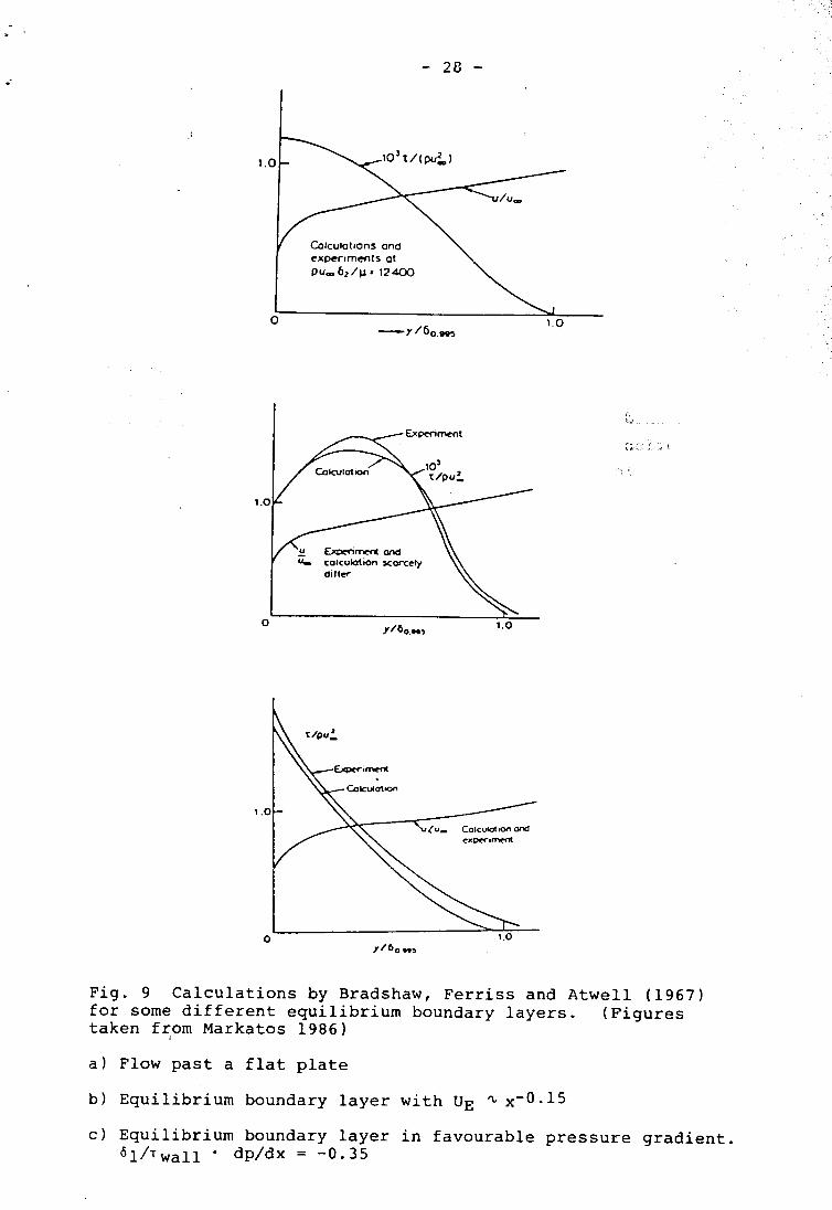
Fig. 9 Calculations by Bradshaw, Ferriss and Atwell (1967)for some different equilibrium boundary layers. (Figurestaken from Markatos 1986)
a) Flow past a flat plate
b) Equilibrium boundary layer with UE ~ x-0.15
c) Equilibrium boundary layer in favourable pressure gradient.°l/Twall. dp/dx = -0.35

- 29 -.
6. TWO-EQUATION MODELS
In many situations the length scale L (characterizing the
larger eddies) is not only dependent on local flow cond-
itions. Considering, for instance, the turbulent flow down-
stream of a grid. The length scale of the turbulence,
which is generated by the grid, is mainly determined by
the dimensions of the grid itself, but is nevertheless
convected downstream along with the fluid. We may therefore
anticipate that a more realistic turbulence model can be
obtained if the length scale L is calculated from a transport
equation (PDE) rather than from some (local) algebraic
expression. Alternatively, a transport equation for the
product kmLn may be considered, where k is still the mean
kinetic energy of the turbulence.
In order to obtain a dependent variable which really re-
flects the physics of the turbulence, several combinations
of k and L have been considered over the years. Some of
the more important proposals are listed below:
Authors Year m n
-
Kolmogorov 1942 ~ -1
Rotta 1951 0 I
Rodi & Spalding 1970 1 1
Rotta 1971 1 1
Ng & Spalding 1972 1 1
Saffman 1970 1 -2
Spalding 1971 1 -2
Davidov 1961 3/2 -1
Harlow & Nakayama 1967 3/2 -1
Hanja1ic & Launder 1972 3/2 -1
Launder & Spalding 1974 3/2 -1
Tabe11 Suggested transport equations for kmLn.

.
- 30 -." -
Some of the combinations of k and L has an obvious physical
interpretation. While the combination considered by Kolmogorov(m = ~ and n = -I) represents a turbulent or eddy-frequence,
the combination with m = 1 and n = -2 represents turbulent
vorticity. The far most popular combination today is m= 3/2 and n = -1, by which the dependent variable is identi-
fied as the dissipation rate of turbulent energy.
6.1 The k-£ model of turbulence
The famous k-£ model is a two-equation model for turbulence,
in which both k and £ are governed by partial differential
equations. Instead of modelling the viscous dissipation
term (34) in the transport equation (3l) for k, the dissi-
pation is obtained from a new transport equation which
exhibits essentially the same form as eq. (3l). The exact
transport equation for £ was derived by Davidov in 1961
and Harlow and Nakayama in 1967. However, the exact terms
on the right-hand side, which contribute to the change
of £ for a fluid element, must be subject to crude modelling.
The derivation of the exact form of the £-equaiton will
therefore be omitted in this text, and only its modelled
form will be presented.
It is important to emphasize that the k-£ model is based
on the generalized eddy-viscosity hypothesis (7), which
relates the unknown Reynolds stresses to the mean flow
field via the eddy viscosity. The momentum equations for
the mean flow (13), which are to be solved along with the
turbulence model, are strongly influenced by the eddy viscos-
ity. Therefore, in order to close the system of equations,
an algebraic expression which relates the eddy viscosity
to k and £ is required.
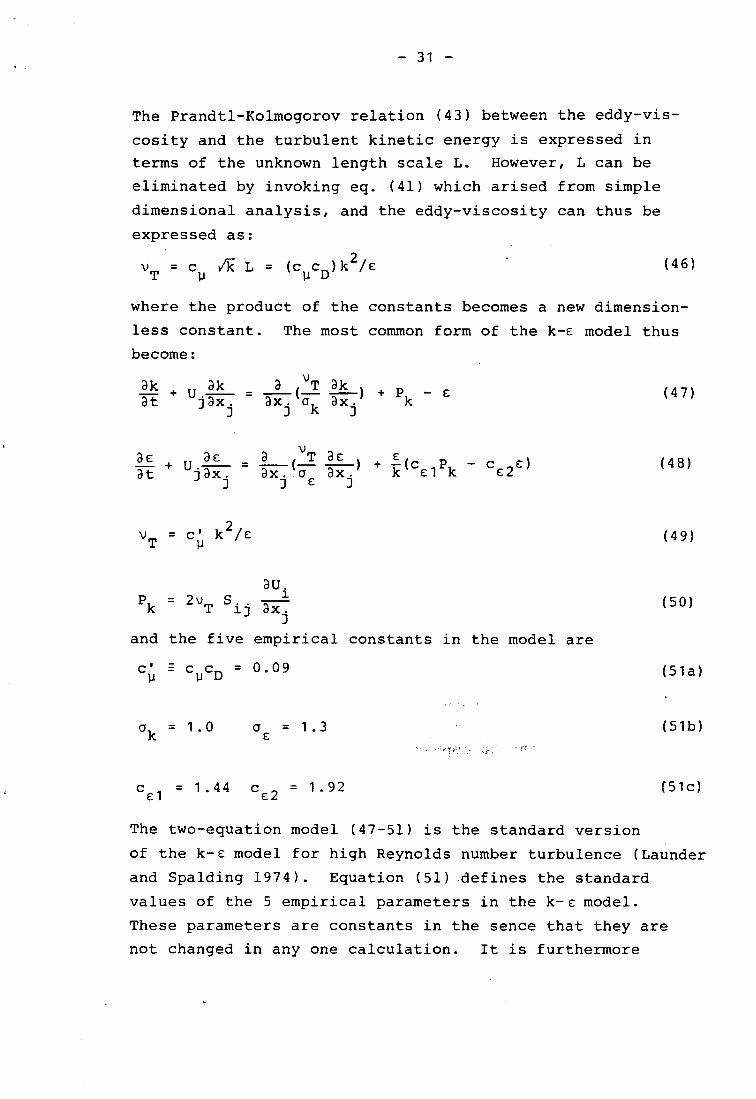
-- 31 -
~
The Prandtl-Kolmogorov relation (43) between the eddy-vis-
cosity and the turbulent kinetic energy is expressed in
terms of the unknown length scale L. However, L can be
eliminated by invoking eq. (41) which arised from simple
dimensional analysis, and the eddy-viscosity can thus be
expressed as:
2v = c /k L = (c c )k IE: (46)T ~ ~ D
where the product of the constants becomes a new dimension-
less constant. The most common form of the k-E: model thus
become:v~ + u.~ = -.:?-(-!~) + p - E: (47)
at J ax. ax. Ok ax. kJ J J
, vaE: aE: a T aE: E: ) ( )at + Uj~ = ax:(cr-~) + k(cE:1Pk - CE:2E: 48
J J E: J
2vT = c~ k IE: (49)
au.1Pk = 2vT S.. ~ (50)
1) ox.J
and the five empirical constants in the model are
c' = c CD = 0.09 (51 a)~ ~
ok = 1.0 °E: = 1.3 (51b)
, :, "
cE1 = 1.44 cE:2 = 1.92 (51c)
The two-equation model (47-51) is the standard version
of the k-E model for high Reynolds number turbulence (Launder
and Spalding 1974). Equation (51) defines the standard
values of the 5 empirical parameters in the k-E: model.
These parameters are constants in the sence that they are
not changed in anyone calculation. It is furthermore

;;
- 32 -." "
to be anticipated that they will not change much from one
flow configuration to another. Modifications of the "cons-
tants" (51) have been proposed in order to account for
low Reynolds number turbulence and such effects as curvature,
rotation and swirl.
The effective Prandtl numbers (51b) are estimated by computer
optimization, while the empirical parameters (51a) and
(51c) are deduced from empirical knowledge about some simple
turbulent flows; i.e. from decay of grid turbulence and
from equilibrium shear layers.
For example, convective transport and diffusion can be
neglected in equilibrium shear layers. Accordingly, the
production of turbulent kinetic energy approximately balances
the dissipation. While the production is given by eq.
(50), the dissipation E can be obtained from eq. (49):
au 2 k2\i (-) = c' - (52 )T ay ~ \iT
Elimination of the eddy viscosity by using eq. (4) gives-2
, ( uv)c~ = k (53)
where both the Reynolds shear stress uv and the turbulent
kinetic energy k are easily measured.
The turbulence model (47-51) together with the continuity
equation and the momentum equation (13) form a closed set
of governing equations which can be solved numerically.
However, in order to solve the model equations we need
a set of boundary conditions. Close to a wall the local
Reynolds number is small and molecular transport mechanism
becomes important. In the standard k-E model, however,'
viscous effects have been neglected and it has become standard
practice to impose boundary conditions at some point near
the wall, but still far enough from it for the direct effects
of viscosity to be negligible. If the dependent variables

.
.:.
- 33 -$
;
in the first computational point near the wall are denoted
by a subscript P, the resulting boundary conditions are:
u u.yUp = ~ R.n(-.:;?!) (54a)
Vp = 0 (54b)
i- 2k = IC' . u (54c)p J.l .
3e:p = U*/KYp (54d)
where Yp is the distance from the wall and u. is the friction
velocity. The boundary conditions (54) are derived by
assuming that the grid point P is located in the fully
turbulent log-law region, where the generation and dissi-
pation of turbulent energy are equal, and where the length
scale is proportional to the distance from the wall.
6.2 Numerical examples
In order to demonstrate the capabilities of the k~ model,
numerical results for some different flow configurations
are presented in this section. First we consider the calcul-
ations by Hackman, Raithby and Strong (1984) for turbulent
flow over a backward-facing step, as shown schematically
in Figure 10. Predicted mean velocity profiles for a laminar
and a turbulent case are shown in Figs. 11 and 12, respectiv-
ely. The predictions are compared with measured data of
Denham and Patric (1974) in the laminar case and experimental
findings of Kim (1978) in the turbulent case. The reattach-
ment length is about 9 step heigths in the laminar case,
and about 7h in the turbulent case. The predicted variation
of the turbulent kinetic energy k and the shear stress
component -uv are shown in Figs. 13 and 14, respectively,
while the variation of the pressure coefficient is shown
in Fig. 15.

~
..
.- 3~ -. ..., AVERAGE INrl;.OW PARAMETERS rOR
VELOCITY IS U KIM'S PROBLEM
H . 0.0762 m
h'0.03BlmH
[ y' 0.1524m - I LZ' 2.338Bm
: --- p . 1.88553 ag/m)I _5
~ . 1.836981 10 ag/m I
h :::::""'- U . 11.B mI.
L I X ,XR I~LI -!. LZ ~
Fig. 10 Backward-facing step flow configuration.
- -- ... 0. !
I
I
2
.c">-
I
0O. '"
U/O
Fig. 11 Mean velocity profiles. Laminar case.
30 KIM
- CARTESIAN- \SHUDS 1421421
\--- CURVILINEAR- IUWDS (421421 ,
2 IIX/h = 1.33 2.67 5.3310 6.22 0 7.11 8.00
.c 0" 0>-
U/U
Fig. 12 Mean velocity profiles. Turbulent case.

~
3 3~---'--- -- ---, '-
I : ,
c. .~r'v""-- Cll~VI..lr;r/.RSHUDS2
2.33 5.89 6.78
0 0.C;
>-
I0 . 0 0.025 . .
k/U2
Fig. 13 Turbulent kinetic energy profiles.
2.33 .~ ~;~~~"':~B9 -- =-cl.C;"->-
. . .
~/U2
Fig. 14 Reynolds shear stress profiles.
o. 0 KIM
-CARTESIAN -SHUDS~ - - KWON a PLETCHERz1../U O.""-"" Z1../ -0 ~ p
u uc. 0. Cp . .-=r, -puc. 2
I../u1%:-:> ."""""""""",'/In -In O. -~ ~a. "L~"" ~ """""
xO. 12
X /h
Fig. 15 Variation of pressure coefficient along the lowerwall downstream of the step.

~-~~-~ ~c",
- 36 -
While the predictions for laminar flow compares favourably
with the experimental data in Fig. 11, some important discre-
pancies are observed in the turbulent case. First, the
calculations underpredict the reattachment length by about
one step height h, depending on the discretization scheme
used for the convective terms. The pred~cted variation
of the pressure coefficient in Fig. 15 is therefore shifted
to the left as compared with the experimental data. Moreover,
the experiments show that the turbulent kinetic energy,
which is generated just downstream of the step corner,
spreads more effectively upwards than indicated by the
predictions in Fig. 13. Finally, the turbulent shear stress
is significantly overpredicted by the turbulence model,
as shown in Fig. 14.
The turbulent flow through a sudden pipe expansion is similar
to the backward-facing step test case, but is obviously
of greater practical relevance. Fig. 16, which together
with Figs. 17-20 have been taken from Rodi's 1980 review,
compares numerical results obtained with ,a one-equation
model and the standard k-E model with experimental data.
It is observed that the k-E model predictions are generally
in better agreement with experimental data than are the
one-equation results.
The k-E model calculations by Durst and Rastogi in Fig.
17 show that the predicted mean velocity profile downstream
of the square obstacle slightly deviates from the measured
velocity profiles. The predictions are otherwise quite
reasonably, and reproduce the two small recirculation zones
in front and top of the block, as well as the large recir-
culation region downstream of the obstacle.
Another example, calculated by Gosman and Young, is the
turbulent flow in a square cavity. Fig. 18 shows the U

- 37 - -~ x 0.5 U/UtT 0 ~~~~"~"O T ' r.'Ts~~ hB:6B~;;;"1;;-~~ '
1EQN.MODEL Ro 6.6 6>. . 0 $ ~Ro 0 PITOT , / ~' " "
6 HOT WIRE /0 0; I" f-1
;::~p"O ~ ,,~ ,,'LiO:4 I~~-o ~~ ~ :6 - , ,,~(f- ,"~60 ,,' ~
0" ,/ ,',' l:,.. 0 ,'f I
0' 0 " 6-0 I A ,0 .0 ' , , ~,. , , 0 , ,n " ,'" , ' ,-
Fig. 16 Mean velocity profiles in sudden pipe expansion.
0 Data=~~=::::~,~~~~~~==!:=:!::::o - C Q I cui a t ion0
0 o i ::::::::::::;;;~~;;;;;;;;;;~;;;;;~;~== c-===-
-2 -1 0 1 2 3 I. 5 6 7 B 9 10) I" x IH
0 stream Ines
y0,
Q
Q
0-3 b) velocity profiles ';iH
Fig. 17 Streamlines and mean velocity profiles in channelobstructed by a square block.
. 0.5
0 0
0 0 V-:11Jr U~ U~ 0
d~
-0.5 0U/U~
0.5 0 0.5 1.0
Fig. 18 Velocity profiles in a siuare cavity.

.
- 38 -
and V velocity profiles predicted along a vertical and
horizontal line, respectively. It can be observed that
the model fails to predict the flow behaviour in the region
where the high-velocity fluid meets the righthand vertical
cavity-wall. Nevertheless, the main features of the flow
are reasonably reproduced.
Finally, we consider some free shear flows, or more speci-
fically, a plane and an axisymmetric wake. Fig. 19 shows
that the k-E model describes the plane wake behind a flat
plate in an excellent manner (also in the upstream region
where the flow is not selfpreserving). In the axisymmetric
wake flow in Figure 20, the ratio of production of turbulent
kinetic energy Pk to its dissipation E is quite low
(~0.15). It is observed that the standard k-E model,
as well as a one-equation k-model and an algebraic mixing-
length model, fail considerably to reproduce the flow develop-
ment. However, if the "constant" c~ in the k-E model is
given as a function of Pk/E, the predictions become more
resonable.
,..-i ~
,

-~C~
r. -~
- 39 - -; .£
. . ~ "
"
- I
- - Predictions Roo. 1'+"2
0 ExperIments- Chevray and Kovasznay (151)
-1
0 xlcmJ 150- O.2.L ,6 11 U/Ue
L
5
x:O x:20cm x:50cm x=150cm7
Initial profileat trollingedge of plate
y(cml
.Fig. 19 Velocity profiles in a plane wake behind a flatplate.
120
( Uo)-3/2 k£model, 8 Expts [152] ~- c =O.09~ ' UE ~ ~80 k£model 8 8
-' 8c~=f(P/E) ---
. . ~ 8 mIxing length -4 . hypothesIs 8 ! - 1- Eq~~-=-
-8_8 - -~:--.-=~ -:- .
0 8 16 40 48 56 64
x/D
Fig. 20 Streamwise variation of maximum velocity defect. in an axisymmetric wake.
- ~~ - - 40 -,
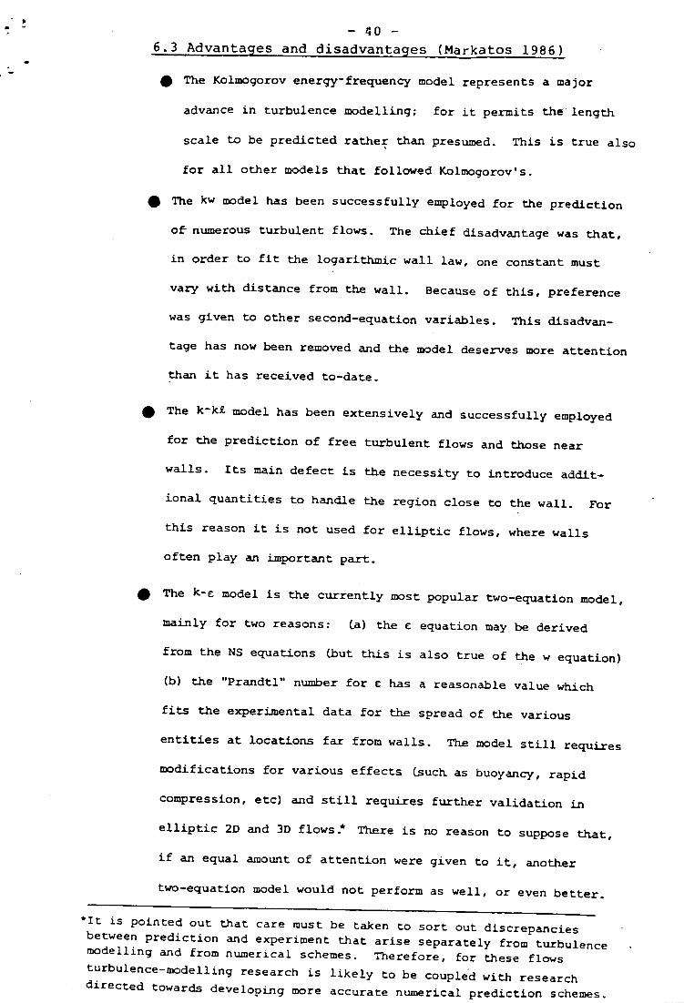
_6.3 Advantaqes and disadvantages (M~katos 1986)
- tt The Kolmogorov energy-frequency model represents a major
advance in turbulence modelling; for it permits the length
scale to be predicted rathef than presumed. This is true also
for all other models that followed Kolmogorov's.
4t The kw model has been successfully employed for the prediction
of- numerous turbulent flows. The chief disadvantage was that,
in order to fit the logarithmic wall law, one constant must
vary with distance from the wall. Because of this, preference
was given to other second-equation variables. This disadvan-
tage has now been removed and the model deserves more attention
than it has received to-date.
4t The k-kl model has been extensively and successfully employed
for the prediction of free turbulent flows and those near
walls. Its main defect is the necessity to introduce addit-
ional quantities to handle the region close to the wall. For
this reason it is not used for elliptic flows, where walls
often play an important part.
~ The k-c model is the currently most popular two-equation model,
mainly for two reasons: La) the c equation may be derived
from the NS equations (but this is also true of the wequation)
(b) the "Prandtl II number for e: has a reasonable value which
fits the experimental data for the spread of the various
entities at locations far from walls. The model still requires
modifications for various effects ~uch as buoyancy, rapid
compression, etc) and still requires further validation in
elliptic 2D and 3D flows.* There is no reason to suppose that,
if an equal amount of attention were given to it, another
two-equation model would not perform as well, or even better.
*It is pointed out that care must be taken to sort out discrepancies
between prediction and experiment that arise separately from turbulence
modelling and from numerical schemes. Therefore, for these flows
turbulence-modelling research is likely to be couple'd with researchdirected towards developing more accurate numerical prediction schemes.

..,
- 41 -
.4t In general,predictions of current transport models (k-~, k-w)
agree fairly well with experimental data for:
. 2D boundary layers and jets along plane walls;
~ . 2D jets, wakes, mixing layers, plumes; ~
. 2D flow in tubes, channels, diffusers and annuli;
. many 3D flows without strong swirl, density variations
or chemical reaction;
. some flows influenced by buoyan.cy and 10w-Reynolds-
number effects.
Ad hoc corrections must be made to the models or to the
"constants" in order to procure agreement with experiments on:-
. boundary layers on convex and concave walls;
. strongly swirling and recirculating flows;
. axi-symmetrical jets in stagnant surroundings;
. 3D wall jets;
. gravity-stratified flows;
. flows involving chemical reactions;
. two-phase flows.
.. Current transport models neglect intermittency (i.e. the
ragged edges of jets and boundary layers), periodicity (i.e.
the eddy-shedding propensity of wakes) and postulate, in
general, gradient-induced diffusion, whereas other diffusion
mechanisms exist. Furthermore, ~e absence of a direct means
of establishing the constants delays progress.
The above disadvantages lead researchers towards more "physical"
models like large-eddy simulation and "two-fluid" models.

.;- "!'i¥':;i;;;~";!
,.
- 42 -
7. REYNOLDS STRESS MODELS
While the algebraic models are based on the assumption of
turbulence in equilibrium, the one- and two-equation models
allow for transport of Qllg turbulent velocity scale. But
models including the turbulent kinetic energy k ~e i~i~ly, fl 1 , ,2 22based on the assumptl.on 0 oca l.sotro~~, l..e. ul = u2 = u3.
In real flows, however, the turbulent energy is usually
produced in one normal stress component, and subsequently
transferred into the other normal stress components.
Anisotropic turbulence can be modelled by separate transportequations for the individual Reynolds-stress components:
r 2 - _1-UI -UlU2 -UlU3
- 1 - 2 _I-UiUj = -U2UI -U2 -U2U3
l - - -:-::T
J-U3UI -U3U2 -U3
therby allowing for different velocity scales for the various
stress components.
Keller and Friedmann suggested in 1924 that the Reynolds
stresses -~. could be obtained from trans port equations,1 Jwhile Chou was the first to derive and publish (in 1945) exact
transport equations for these stress components. The following
procedure may be used:
1) Consider the xi-component of the Navier-Stokes equations.
2) Subtract the xi-component of the Reynolds-averaged N-S.
3) Multiply by Uj.
4) Change indices i and j in the equation from step 3).
5) Add results from step 3) and 4).
6) The result is then Reynolds-averaged, and can be written
as:

."-
- 43 -, .'"
D U"-:u.---1--1 = p.. + <1>.. + D.. - E..
Dt 1J 1J 1J 1J
where the left-hand-side represents change of ~ for a fluid
element. The terms on the right-hand-side are:
aU. au.= --:.L - 1Pij - - Uiuk ax - UjUk -a;:-k k
* production of ~ due to mean strain1 J
P au. au.<1>.. ::: -(--1 + -::l.)
1J P ax. ax.J 1
* pressure-strain correlation
- a 1 -r 1 -rD.. = - -[U.U.U k + - pU.u.. + - Pu.u. kJ1J ax. 1 J P J 1J P 1 J
J
* diffusive term
au. au.E .. ::: 2v --1 --.:::.l
1J ax axk. k.
* dissipative term. The spatial derviatives of the fluctuating
velocity components are so large that the dissipation cannot
be neglected.
It can be demonstrated that the transport equation for
the Reynolds stresses contracts (~.e. summation of the
equations for the 3 normal stresses) to the exact transport
equation for the mean turbulent kinetic energy. In this case
the contributions from the pressure-strain correlations
disappear. These terms do not change the turbulent kinetic
energy, but tend to redistribute energy between the different
normal stress components. Note that <1>11' <1>22' and <1>33 all can benonzero, while the sum <1>.. = o.
11
The production terms Pij are made up of Reynolds stress
components and gradients of the mean velocity field. No

...
- 44 -
approximations are required for these important terms at thislevel of modelling. The other right-hand-side terms, however,
must be subject to modelling, and a set of partial
differential equations are obtained. This kind of turbulence
models is called Differential Stress Models (DSM). In a
general 3-dimensional case, 6 PDE's for the Reynolds stresses ~
are solved together with a PDE for the energy dissipation
rate.
A somewhat simpler class of Reynolds stress models, which
still retains some of the important features of the DSM-
models, is the Algebraic Stress Models (ASM). In this
approach, alternative modelling assumptions are used for all
terms in the DSM model which involve spatial derivatives of
the Reynolds stresses. Thus, an algebraic set of relationships
between the stresses can be derived, which subsequently is
used together with PDE's for the mean turbulent kinetic energy
(k) and its dissipation rate (E).
The accompanying figure shows numerical calculations by
Sultanian, Neitzel & Metzer (1985) of the flow through an
axisymmetric expansion (i.e. a pipe with sudden increase in
diameter). Streamwise mean velocity profiles are shown at
different cross-sections downstream of the expansion for the
case Re=60000, and it is observed that the results obtained
with an ASM model (solid line) compare more favourably with
the experimental points than the calculations (broken lines)
with the standard k-E model.
The Reynolds stress models, DSM and ASM, are today the
most complete and accurate representation of turbulence which
are used in technological applications. Their major advantage
is the exact evaluation of the crucial production terms. The
most general models can be gradually reduced to decrease the
computational time without significantly loss of accuracy.
ASMs, for instance, represent a powerful compromise between
full DSMs and the k-E model in complexity and applicability.

~:"-?;:';,c,;,;,,-::;r:i~i!~]7"'"
,- 45 - - ...
- " ;!
1.O.
4x/D1 = 2 x/D1 = 3 x/D1 =O.
O.
O.
r/R2 O.
O.
O.
O.
O.
0 . .U/U,
1.
O. (U1 = 1.13m/s)
O. x/D1 = 6 x/D, = 8 x/D1 = 10 x/D1 = 12
O.
O.
r/R2 O.
O.
0
0
0..
. 1.0 0 0
U/U,
Fig. 21 Mean axial velocity profiles downstream of an
axisymmetric expansion.