
Failure time data modeling and analysis APPROVED BY ...
58
The Report committee for Chen Zhu Certifies that this is the approved version of the following report: Equipment data analysis study ---- Failure time data modeling and analysis APPROVED BY SUPERVISING COMMITTEE: Supervisor: _______________________________ Elmira Popova ________________________________ J.Eric Bickel
Transcript of Failure time data modeling and analysis APPROVED BY ...

The Report committee for Chen Zhu
Certifies that this is the approved version of the following report:
Equipment data analysis study
---- Failure time data modeling and analysis
APPROVED BY
SUPERVISING COMMITTEE:
Supervisor: _______________________________
Elmira Popova
________________________________
J.Eric Bickel
Equipment data analysis study
----- Failure time data modeling and analysis
by
Chen Zhu, B.E.
Report
Presented to the Faculty of the Graduate School
of the University of Texas at Austin
in Partial Fulfillment
of the Requirements
for the Degree of
Master of Science in Engineering
The University of Texas at Austin
May 2012

iii
Acknowledgement
I wish to express my sincere gratitude to my supervisor, Prof. Elmira Popova,
Department of Operations Research and Industrial Engineering, University of
Texas at Austin for her support and guidance in carrying out this report. Also, I
sincerely thank to my second reader, Prof. J. Eric Bickel and I wish to express my
gratitude to Liang Sun, Duc Viet Nguyen and Ying Chen who rendered their help
during the period of my report work. Last but not least I thank my beloved parents
and all my friends for their manual support, strength, help and for everything.
iv
Equipment data analysis study
---- Failure time data modeling and analysis
by
Chen Zhu, M.S.E
The University of Texas at Austin, 2012
SUPERVISOR: Elmira Popova
This report presents the descriptive data analysis and failure time modeling that can be
used to find out the characteristics and pattern of failure time. Descriptive data analysis
includes the mean, median, 1st quartile, 3
rd quartile, frequency, standard deviation,
skewness, kurtosis, minimum, maximum and range. Models like exponential distribution,
gamma distribution, normal distribution, lognormal distribution, Weibull distribution and
log-logistic distribution have been studied for failure time data. The data in this report
comes from the South Texas Project that was collected during the last 40 years. We
generated more than 1000 groups for STP failure time data based on Mfg Part Number.
In all, the top twelve groups of failure time data have been selected as the study group.
For each group, we were able to perform different models and obtain the parameters. The
significant level and p-value were gained by Kolmogorov-Smirnov test, which is a
method of goodness of fit test that represents how well the distribution fits the data. The
In this report, Weibull distribution has been proved as the most appropriate model for
STP dataset. Among twelve groups, eight groups come from Weibull distribution. In
general, Weibull distribution is powerful in failure time modeling.

v
Table of Contents
List of Tables……………………………………………………………..... vi
List of Figures…………………………………………………………...…vii
1. Introduction……………………………………………………………….1
2. Literature Review……………………………………………………........3
3. Problem Statement …… … ……………………………………………...5
3.1 Failure time distribution ………………………………………………..5
3.2 The Exponential distribution ……………………………………………5
3.3 The Gamma distribution ……………………………………………….. 6
3.4 The Weibull distribution ……………………………………………….. 6
3.5 The Normal distribution ………………………………………………..7
3.6 The Lognormal distribution ………………………………… …………7
3.7 The Log-Logistic distribution ………………………………………….. 8
4. Solution Methodologies and Analysis……………………………………9
4.1 Preliminary data analysis ……………………………………………….9
4.2 Maximum Likelihood Estimation……………………………………….10
4.3 Goodness of Fit Test …………………………………………………..11
5. Computational Results…………………………………………………..12
5.1 Data preparation and description………………………………………. 12
5.2Descriptive data analysis ……………………………………………….13
5.3 Failure time model……………………………………………………..15
6. Conclusions……………………………………………………………...23
7. References……………………………………………………………….48

vi
List of Tables
Table 1. South Texas Project Data Dictionary ………………………………..13
Table 2. Data groups based on Mfg Part No…………………………………..14
Table 3. Descriptive data analysis for failure time of twelve groups ………….15
Table 4. Distribution fitting results forGroup1………………………………...16
Table 5. Distribution fitting results forGroup2………………………………...17
Table 6. Distribution fitting results forGroup3………………………………...17
Table 7. Distribution fitting results forGroup4………………………………...18
Table 8. Distribution fitting results forGroup5………………………………...18
Table 9. Distribution fitting results forGroup6………………………………...19
Table 10. Distribution fitting results forGroup7 ………………………………19
Table 11. Distribution fitting results forGroup8 ………………………………20
Table 12. Distribution fitting results forGroup9 ………………………………20
Table 13. Distribution fitting results forGroup10 ……………………………21
Table 14. Distribution fitting results forGroup11 ……………………………21
Table 15. Distribution fitting results forGroup12 ……………………………22
vii
List of Figures
Figure 1. Histogram for Group 1……………………………………………..24
Figure 2. Histogram for Group 2……………………………………………..24
Figure 3. Histogram for Group 3……………………………………………..25
Figure 4. Histogram for Group 4……………………………………………..25
Figure 5. Histogram for Group 5……………………………………………..26
Figure 6. Histogram for Group 6……………………………………………..26
Figure 7. Histogram for Group 7……………………………………………..27
Figure 8. Histogram for Group 8……………………………………………..27
Figure 9. Histogram for Group 9……………………………………………..28
Figure 10. Histogram for Group 10…………………………………………..28
Figure 11. Histogram for Group 11…………………………………………..29
Figure 12. Histogram for Group 12…………………………………………..29
Figure 13.Weibull distribution fitting for Group1……………………………..30
Figure 14.Weibull distribution fitting for Group2……………………………..30
Figure 15.Weibull distribution fitting for Group3……………………………..31
Figure 16.Weibull distribution fitting for Group4……………………………..31
Figure 17.Weibull distribution fitting for Group5……………………………..32
Figure 18.Weibull distribution fitting for Group6……………………………..32
Figure 19.Weibull distribution fitting for Group7……………………………..33
Figure 20.Weibull distribution fitting for Group8……………………………..33
Figure 21.Weibull distribution fitting for Group9……………………………..34
Figure 22.Weibull distribution fitting for Group10 ………………………….. 34
Figure 23.Weibull distribution fitting for Group11 ………………………….. 35
Figure 24.Weibull distribution fitting for Group12 ………………………….. 35
viii
Figure 25.Failure time vs. unreliability plot for Group1…………………….. 36
Figure 26.Failure time vs. unreliability plot for Group2…………………….. 36
Figure 27.Failure time vs. unreliability plot for Group3…………………….. 37
Figure 28.Failure time vs. unreliability plot for Group4…………………….. 37
Figure 29.Failure time vs. unreliability plot for Group5…………………….. 38
Figure 30.Failure time vs. unreliability plot for Group6…………………….. 38
Figure 31.Failure time vs. unreliability plot for Group7…………………….. 39
Figure 32.Failure time vs. unreliability plot for Group8…………………….. 39
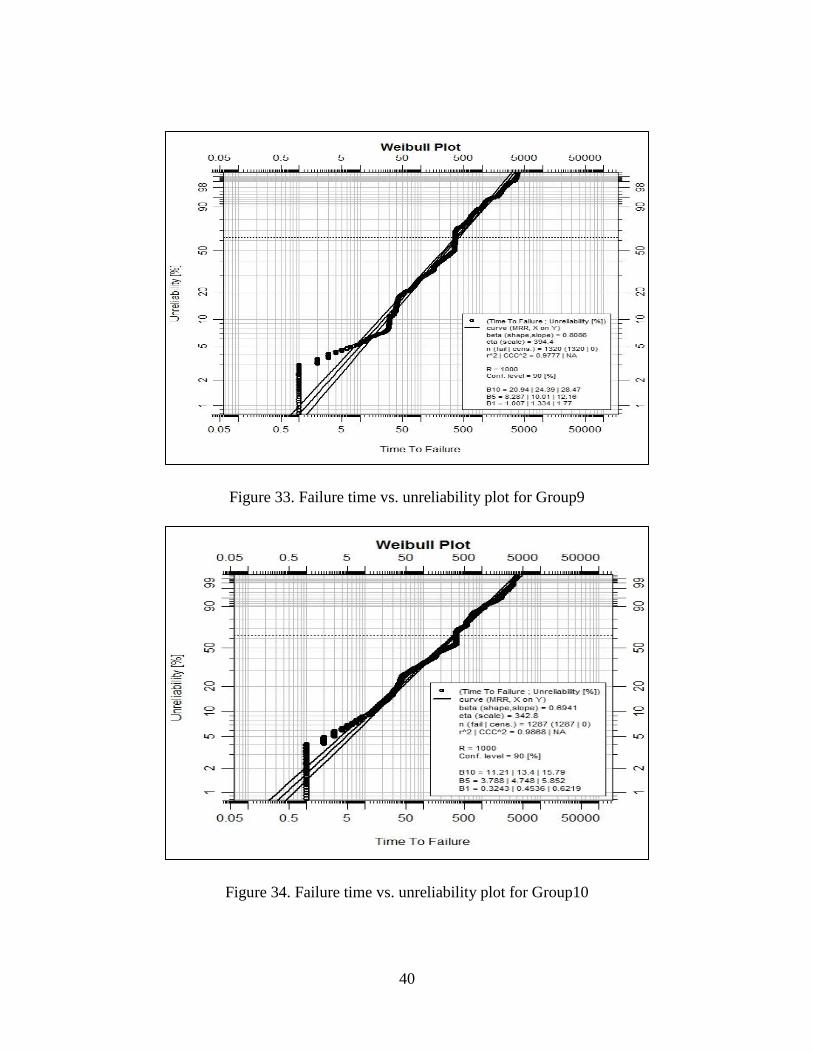
Figure 33.Failure time vs. unreliability plot for Group9 ……………………. 40
Figure 34.Failure time vs. unreliability plot for Group10…………………… 40
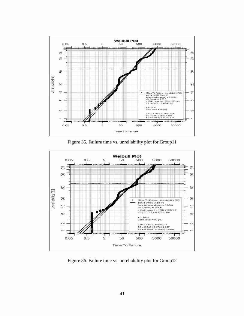
Figure 35.Failure time vs. unreliability plot for Group11…………………… 41
Figure 36.Failure time vs. unreliability plot for Group12…………………… 41
Figure 37.Weibull GOF test for Group1…………………………………… 42
Figure 38.Weibull GOF test for Group2…………………………………….42
Figure 39.Weibull GOF test for Group3…………………………………….43
Figure 40.Weibull GOF test for Group4…………………………………….43
Figure 41.Weibull GOF test for Group5…………………………………….44
Figure 42.Weibull GOF test for Group6…………………………………….44
Figure 43.Weibull GOF test for Group7…………………………………….45
Figure 44.Weibull GOF test for Group8…………………………………….45
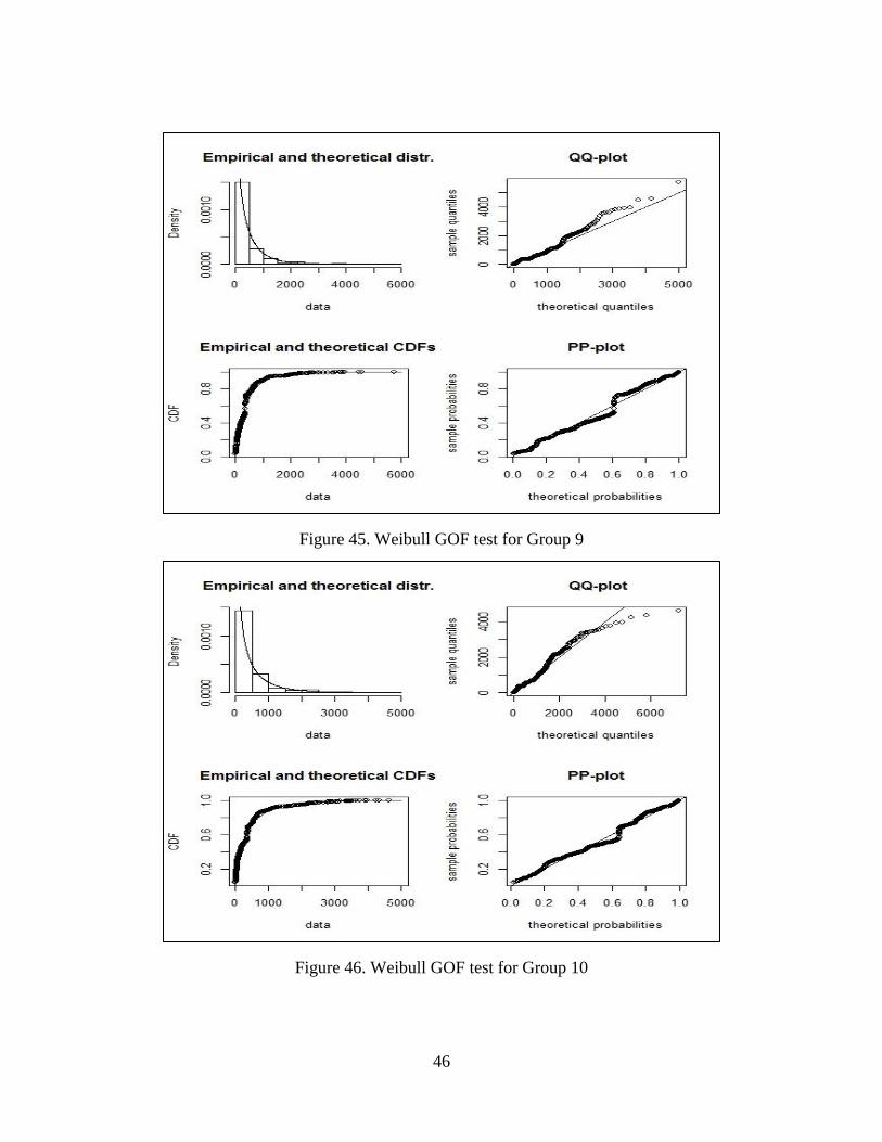
Figure 45.Weibull GOF test for Group9…………………………………….46
Figure 46.Weibull GOF test for Group10……………………………………46
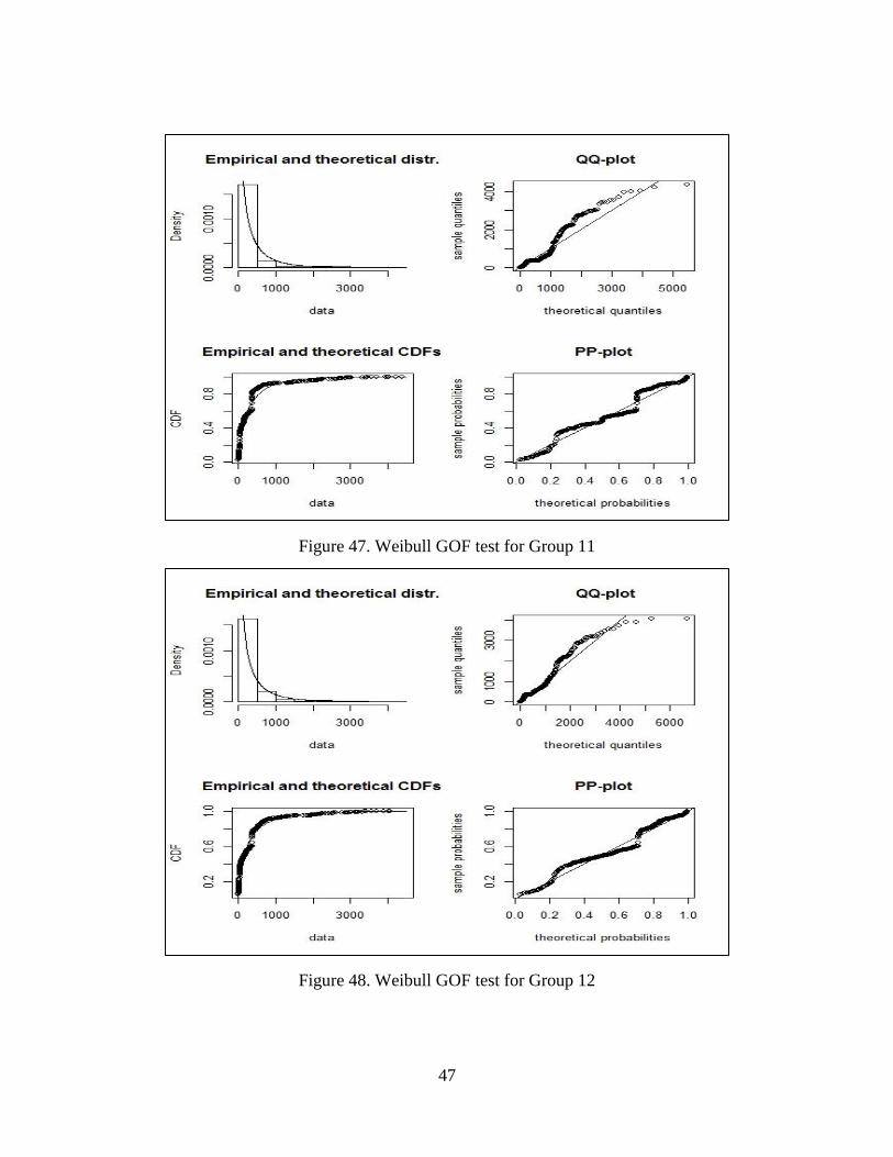
Figure 47.Weibull GOF test for Group11……………………………………47
Figure 48.Weibull GOF test for Group12……………………………………47

1
1. Introduction
Reliability study is a field that deals with the quality, safety and availability of a system.
It has been widely applied in risk analysis, environmental protection, optimization of
maintenance and operation, quality control and engineering design. The time between
failures, failure frequencies, the probability of failure are the major object of reliability
study. Norman came up with that the failure time analysis is a critical part in the study of
the system reliability (Knight 1991). Leslie, Timothy, Frank, Halima and Ramon (2008)
pointed out that failure time data analysis
Failure time analysis is a method of data analysis which aims to discover the
cause of for the failure of a component or a device. In failure time analysis, the response
is the time between two failures. It is always compared to the survival analysis which is
defined as the method to analyze survival time such as after a certain time, how many
people or systems will survival. There are two basic problems in failure time analysis.
One problem involves the assessment of the dependence between the failure time and the
explanatory variables. The other one is how to model and estimate the distribution of the
failure time. Some other problems that arise in the failure time analysis include
assessment of failure frequency (Kalbfleish and Prentice 2011).
In our data, the time between two failures can be really short which increase the
repair cost and thus increase the total cost. It is important to analyze the failure time and
find out the pattern. In this report, we conducted the preliminary data analysis of the
failure time and failure time modeling. We presented a wide range of models that can be
used to solve the failure time distribution fitting problem. But we only focused on the six
most popular distributions used in the failure time study that is normal, exponential, log-
logistic, gamma, Weibull and lognormal. Because of the properties of failure time data,
there will be some individuals that do not fail during the time being observed. Especially
sometimes the experiment has an upper test duration limit. This kind of specimen being
taken from the tested is categorized as right censored data. In our dataset, the failure time
is collected by the mechanical-dynamical testing method, which means there are only a
few specimen being tested thus it is completely uncensored data(Jurgen and Filip 2011).

2
In the second section, we review the literature related to failure time analysis and
reliability study. A description of failure time analysis is given in Section3 that includes
distribution fitting and failure time properties. In Section4 we provide the specific
problem statement and models. In Section 5, we give an example and present our
computational results obtained with R12.1 and South Texas project data sets tested.
Dataset includes twelve groups of data collected during the past 40 years with different
attributes. We close with a summary of the work and suggestions for future research.

3
2. Literature Review
Failure time analysis is commonly used in the field of industrial life testing. But it is not
unique to that industry. Actually the failure time problem is a part of reliability problem.
There is a vast majority of literature on the study of reliability. Gilbert and Sun (2005)
has introduced one kind of failure time analysis which can apply to HIV vaccine effect on
antiretroviral therapy. They consider methods of using a surrogate endpoint that can be
assessed by standard survival analysis techniques.
In the study of failure time analysis on time models, Johnson and Kotz (1970)
introduce some certain parametric models such as exponential and Weibull models. Log-
normal and gamma distribution are mentioned by Mantel, N and Byar, D.P. (1974).
Lawless (1982) gives a more detailed explanation about those various models. He
illustrates the exponential, gamma, lognormal, log-logistics, log-location-scale and
Weibull distribution and how they work in the lifetime data. In his literature, he also
mentions mixture models which are not frequently used, however, sometimes can be
really efficient. The other parametric models for failure time study such as log F is
mentioned by Kalbfleisch and Prentice (2011). In recent years, compound distribution
has been widely used. David D. Hanagal (2010) comes up with using compound passion
distribution to model bivariate survival data.
Weibull distribution has demonstrated its usefulness in a wide range of situations
in failure time study. In terms of the univariate models, Weibull is the most widely used
in failure time model. Dodson (2006) aims at introducing two- parameter Weibull model
into fatigue and reliability analysis. He focus on predict failure times of products by using
Weibull distribution and point out that Weibull distribution is powerful in terms of
widely application. Chi (1997) said that unless it has strong evidence that the life time
data fit in another distribution, Weibull distribution should be considered as the principal
fitting distribution. In the recent years, there are a growing number of lifetime data
studies that focus on combining Weibull and other distribution together. K.W.Fertig
(1972) conducts the Bayesian Weibull analysis for lifetime data. In the study, instead of

4
using the constant failure rate, it describe a time varying one by modeling the time
between failures as Weibull random variables.
Some other literature focuses on the study of logmormal and gamma distribution.
It has been proved that lognormal distribution works well on the nonconstant
instantaneous failure rates, which also implies that the logarithms of lifetime are normally
distributed. Eckhard, Werner and Markus (2001) give a clear explanation about the
application of lognormal distribution. It is useful when we analyze the reliability if the
devices. Gamma distribution has been applied on the cluster lifetime data. Joanna and
Thomas (1994) refer that gamma frailty model is a good way to model clustered failure
time data.

5
3. Problem Statement
In this report, we focus on the preliminary data analysis and lifetime modeling. There is a
vast range of statistic knowledge applied in failure data analysis. The basic quantitative
measures are failure time distribution and failure rate function, through which scientists
inspect the reliability of systems (John and Ross 2011). Several standard parametric
models for homogeneous lifetime data analysis has been constantly used including
exponential distribution, Weibull distribution, gamma distribution, normal distribution,
lognormal distribution and log-logistic distribution (Lawless, Jerald F.1982).
3.1 Failure time distribution
Unless stated, the time to failure T is defined as a continuously variable. Let ( ) denote
the probability density function. The following function is the distribution function of T.
( ) ( ) ∫ ( )
The probability of an item dose not fail to time t is defined by
( ) ( ) ( ) ∫ ( )∞
The failure rate function is defined as
( | )
This function is also called hazard function. It specifies the event rate on the condition
that an item has survived at least until time T (Willis Jackie 2005).
3.2 The Exponential Distribution
If the time between failures has the probability density function
( ) {
We call this one parameter distribution as exponential distribution with parameter . It
also implies that the hazard function is constant over the time interval. Thus the event rate
is independent of t. The failure rate is
6
( ) ( )
( )
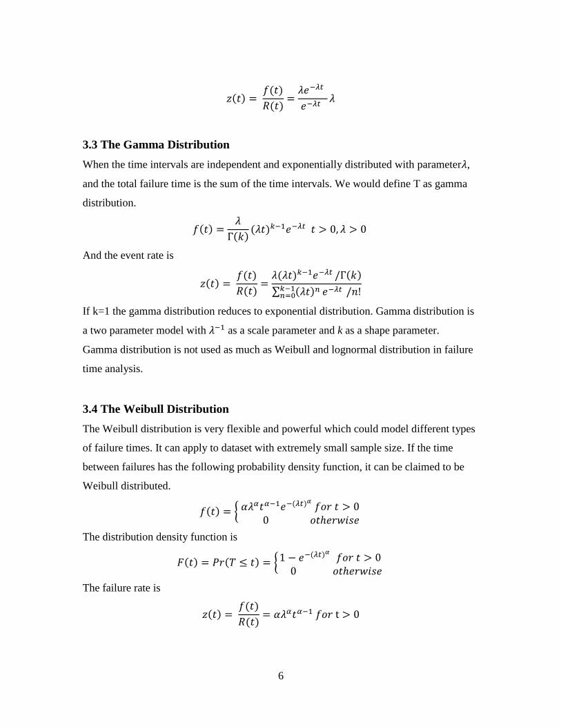
3.3 The Gamma Distribution
When the time intervals are independent and exponentially distributed with parameter ,
and the total failure time is the sum of the time intervals. We would define T as gamma
distribution.
( )
( )( )
And the event rate is
( ) ( )
( )
( ) ( )
∑ ( )
If k=1 the gamma distribution reduces to exponential distribution. Gamma distribution is
a two parameter model with as a scale parameter and k as a shape parameter.
Gamma distribution is not used as much as Weibull and lognormal distribution in failure
time analysis.
3.4 The Weibull Distribution
The Weibull distribution is very flexible and powerful which could model different types
of failure times. It can apply to dataset with extremely small sample size. If the time
between failures has the following probability density function, it can be claimed to be
Weibull distributed.
( ) { ( )
The distribution density function is
( ) ( ) { ( )
The failure rate is
( ) ( )
( )

7
In Weibull distribution, affects the location of the pattern and affect the scale of the
distribution. If the failure rate is constant, if event rate function is increasing
and if , it is decreasing.
3.5 The Normal Distribution
The normal distribution is the most commonly used model in statistical study.
A variable T is normally distributed as ( ) if it has the probability density
function
( )
√ ( )
The hazard function is
( ) ( )
( )
(
)
(
)
Normal distribution is not as popular as lognormal and log-logistic distribution in failure
time analysis.
3.6 The Lognormal Distribution
Scientists have used lognormal distribution in diverse fields such as engineering and
medicine. In this report, lognormal is one of the main measures for the failure time study.
The time between failures has the probability density function
( ) {
√ ( )
It is said to be lognormally distributed with parameters and . We can get
that is normally distributed with mean and variance .
The hazard function for lognormal distribution is
( ) (( ) )
(( ) ) )
where ( ) denotes the probability density of the standard normal distribution.

8
3.7 The Log-Logistic Distribution
The log-logistic distribution comes from the fact that is logistically
distributed. It has similar shape with normal distribution. When the lifetime data has the
probability density function
( ) ( )(
)
( )
The failure rate function is
( ) ( )(
)
( )

9
4. Solution Methodologies and Analysis
For this failure time dataset, one of our objectives is to perform the preliminary data
analysis to find out the characteristics of data. Scientists have pointed out different
methods that are efficient to study the pattern. The preliminary data analysis is a basic
but useful tool. After we conducted preliminary data analysis, we obtained the parameter
of the distribution using maximum likelihood estimation method and conducted the
goodness of fit test.
4.1 Preliminary data analysis
Preliminary data analysis provides a way for scientists to learn the basic statistical
properties of the dataset. And it includes a vast range of statistic methodologies, which
allows analysts find out the pattern of data and thus narrow down the scope of the
research. The most powerful and widely used method is descriptive data analysis
(Werner and Reinhard 1996).
Descriptive analysis summarizes the data from our studies. It is used to give a
description of the data including measuring the location and variability. In the aspect of
measuring the location, it offers median, mode and mean whose properties are used to
identify the outliers, the general information about data. Median is an indication of the
value in the central location. Mean is the average of the data. Because it is sensitive to
individual observation, one extreme large data can contribute to a lot to the mean.
Sometimes we use median and mean together to detect outliers of the dataset. Variation is
a measure of data spread. It will give us how data has been spread out around the mean.
Maximum and minimum are basic information about the dataset range. Kurtosis
compares the shape of the distribution to the normal one. If the kurtosis value is high, the
data is peaked and if the value is low, the data is flat. Skewness gives the information
about whether this data is symmetric or not. Value of skewness equals to zero means this
data are symmetrical (Willis Jackie 2005).
The frequency distribution has been introduced to catch some characteristics of
the population. Frequency distribution could be obtained by grouping data in terms of
their levels and forming the distribution of different groups. It often uses bar charts
10
(histogram) to represent the frequency of data and we will draw a line that connects the
midpoints of bars. More bars can lead to more accurate and smooth curve which is an
easy way to find out the distribution characteristics visually. Thus, through the histogram,
first, it gives the frequency of each group. Second we can get the basic assumption of the
data distribution and then use other techniques to test it. In this report, we study the
failure time pattern by modeling its frequency distribution. There are some basic
concerns about distribution fitting. For example, which distribution the data comes from,
how to determine the parameters, if the data fits more than one distribution, which one is
the best. To solve these problems, we introduce the maximum likelihood estimation and
goodness of fit test in the following paragraphs.
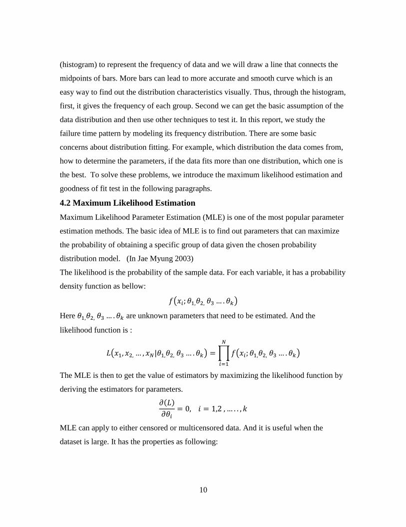
4.2 Maximum Likelihood Estimation
Maximum Likelihood Parameter Estimation (MLE) is one of the most popular parameter
estimation methods. The basic idea of MLE is to find out parameters that can maximize
the probability of obtaining a specific group of data given the chosen probability
distribution model. (In Jae Myung 2003)
The likelihood is the probability of the sample data. For each variable, it has a probability
density function as bellow:
( )
Here are unknown parameters that need to be estimated. And the
likelihood function is :
( | ) ∏ ( )
The MLE is then to get the value of estimators by maximizing the likelihood function by
deriving the estimators for parameters.
( )
MLE can apply to either censored or multicensored data. And it is useful when the
dataset is large. It has the properties as following:
11
MLE is approximately normally distributed.MLE is approximately minimum variance
and as sample size grows, the variance becomes smaller. MLE is approximately
unbiased. (George and Roger 2001)
4.3 Goodness of Fit Test
The goodness of fit is a statistical model describes how well it fits a set of observations
(Wikipedia). The goodness of fit test starts to calculate the distance between the null
hypothesis and the alternative hypothesis. It will give a probability (p value) which is the
probability of observing data at least as extreme as what we did in the direction predicted
by , assuming that the null hypothesis is true. Sometimes, the p value is too high to
happen in that way which indicates there are some mistakes like the distribution is over
fitting. There are three methods that are applied very often in the goodness of fit test.
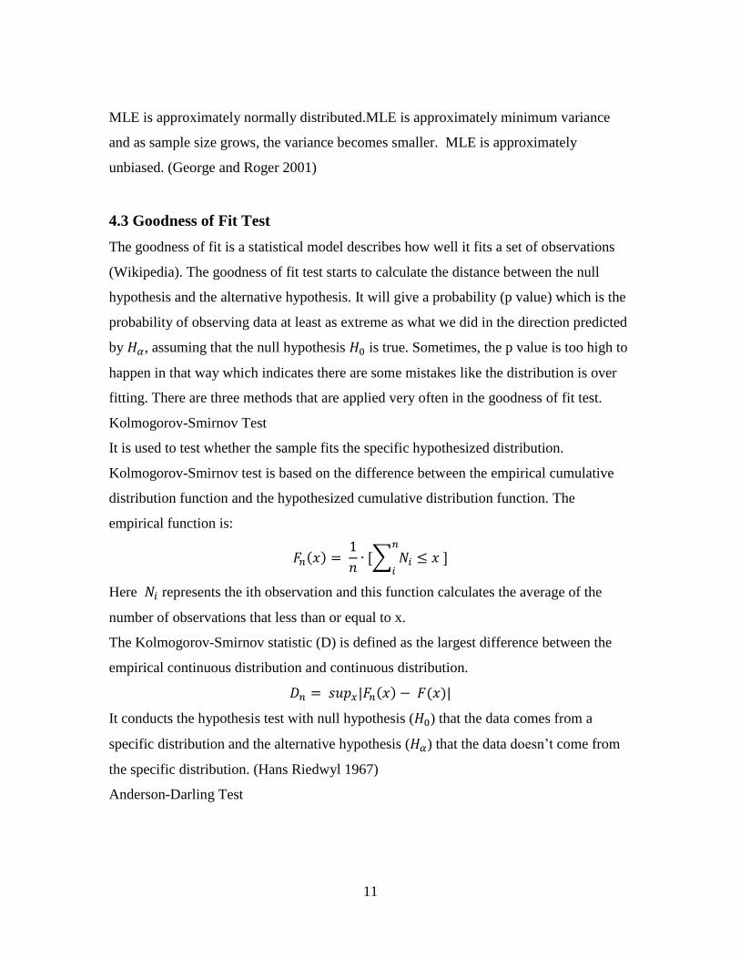
Kolmogorov-Smirnov Test
It is used to test whether the sample fits the specific hypothesized distribution.
Kolmogorov-Smirnov test is based on the difference between the empirical cumulative
distribution function and the hypothesized cumulative distribution function. The
empirical function is:
( )
∑
Here represents the ith observation and this function calculates the average of the
number of observations that less than or equal to x.
The Kolmogorov-Smirnov statistic (D) is defined as the largest difference between the
empirical continuous distribution and continuous distribution.
| ( ) ( )|
It conducts the hypothesis test with null hypothesis ( ) that the data comes from a
specific distribution and the alternative hypothesis ( ) that the data doesn’t come from
the specific distribution. (Hans Riedwyl 1967)
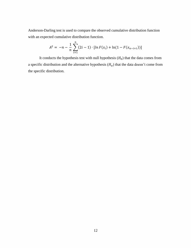
Anderson-Darling Test
12
Anderson-Darling test is used to compare the observed cumulative distribution function
with an expected cumulative distribution function.
∑( )
( ) ( ( ))
It conducts the hypothesis test with null hypothesis ( ) that the data comes from
a specific distribution and the alternative hypothesis ( ) that the data doesn’t come from
the specific distribution.

13
5. Computational Results
5.1 Date preparation and description
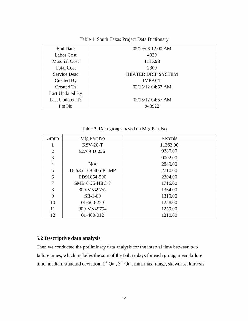
The South Texas project file contains 132056 records and 25 variables. Table 1 gives the
data dictionary and representative records. Mfg Part No is one of the most important
properties to identify machines. In order to find out the characteristics of different
machines, we grouped the data by their Mfg Part No. First, we sorted the data using Mfg
Part No as a key. In this report, we only study the top twelve groups which include most
of records of the dataset. Table 2 shows the Mfg Part No of the top twelve groups and the
number of records in each group. Then we created a new variable called failure time to
represent the interval time between two failure times for a specific record. Excel
provides a way to calculate the days between two dates. It will transfer the start date and
the end date to days to a system specific date. Thus it is not important what date is
defined as a system specific date since we calculate the interval time. Table 3 provides
the preliminary data analysis of twelve groups.
Table 1. South Texas Project Data Dictionary
Column name Records
Tpns Cost Seq No 501,600 502,288
Tagtpns 1HDSYSTEM 8S172XHD0675 N1HDHS7350
System Code HD CC EW
Source WO
Cr No 08-9005-2
Wo No 360280
Surveillance Seq No 87000098
Request Type CRWO
Unit 1
Gqa Risk NRS
Pg Risk NRS LOW
Psa Risk LOW
Mfg Part No CR2940US203E
Mdmfr Mfr Name DIETERICH STANDARD
Start Date 05/28/08 01:21 PM
14
Table 1. South Texas Project Data Dictionary
End Date 05/19/08 12:00 AM
Labor Cost 4020
Material Cost 1116.98
Total Cost 2300
Service Desc HEATER DRIP SYSTEM
Created By IMPACT
Created Ts 02/15/12 04:57 AM
Last Updated By
Last Updated Ts 02/15/12 04:57 AM
Pm No 943922
Table 2. Data groups based on Mfg Part No
Group Mfg Part No Records
1 KSV-20-T 11362.00
2 52769-D-226 9280.00
3 9002.00
4 N/A 2849.00
5 16-536-168-406-PUMP 2710.00
6 PD91854-500 2304.00
7 SMB-0-25-HBC-3 1716.00
8 300-VN49752 1364.00
9 SB-1-60 1319.00
10 01-600-230 1288.00
11 300-VN49754 1259.00
12 01-400-012 1210.00
5.2 Descriptive data analysis
Then we conducted the preliminary data analysis for the interval time between two
failure times, which includes the sum of the failure days for each group, mean failure
time, median, standard deviation, 1st Qu., 3
rd Qu., min, max, range, skewness, kurtosis.

15
Table 3. Descriptive data analysis for failure time of twelve groups
Group Sum Mean Median St.Deviation 1st Qu 3
rd Qu. Min Max Range Skewness Kurtosis
1 3901653 343.8 164.00 560.5039 36.92 368.70 1 4372 4371 3.50382 17.2098
2 1984900 213.9 48.24 393.8428 35.92 364.8 1 4198 4197 5.4261 40.3891
3 2754494 306.0 78.95 598.5372 19.36 286.7 1 5749 5748 3.4585 16.4807
4 2152203 755.2 549.0 770.7545 166.4 1032
1 4664 4663 1.69595 6.1823
5 574589.2 211.9 40.0 514.4802 22.34 168.1 1 7050 7049 4.62899 30.5309
6 343060.9 148.8 50.62 360.3563 8.765 129.5 1 3625 3624 5.74345 41.8807
7 755171.4 439.8 359.9 605.3985 91.15 372.9 1 4012 4011 3.06317 13.4906
8 493898.3 361.8 163 597.8398 38.91 368.8 1 4224 4223 3.10439 13.5654
9 582939.3 441.6 347.8 597.3751 84 493.2 1 5747 5746 3.44758 18.9842
10 585447.9 454.2 264 670.2445 41.92 546 1 4635 4634 2.86416 12.2962
11 457330.2 363.0 165 618.2659 39.91 368.9 1 4379 4378 3.38589 15.5600
12 442706.9 157 365.6 607.9821 30.15 371.4 1 4077 4076 3.26529 14.9576

16
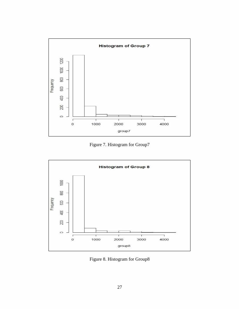
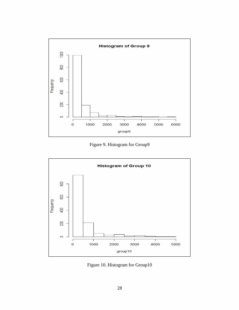
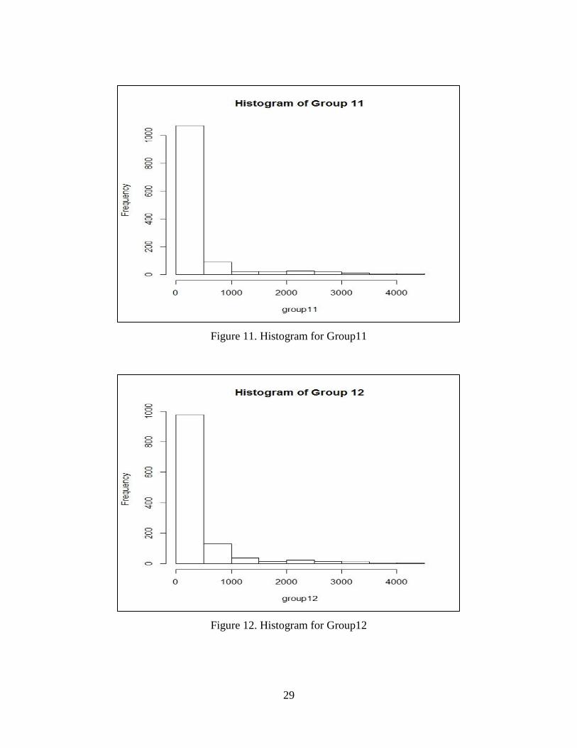
It can be seen from the preliminary data analysis table, the failure time of group 5, group
7, group8, group9 and group10 is large. And the medians of these twelve groups are
much less than their means. Especially the medians of the group2, group5 and group6 are
less than half of their means, which indicates that the data shows a tendency to the y axis.
Group 4 has a large mean comparing to other groups. And the standard deviation for
these twelve groups is pretty large. Group 4 shows a more symmetrical and flat
distribution shape than the other groups. Group 2 and group 6 have high kurtosis value
which indicates the patterns of the data are peaked.
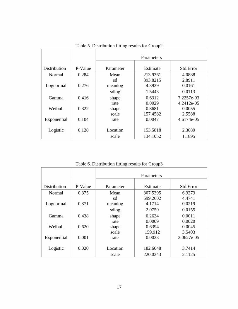
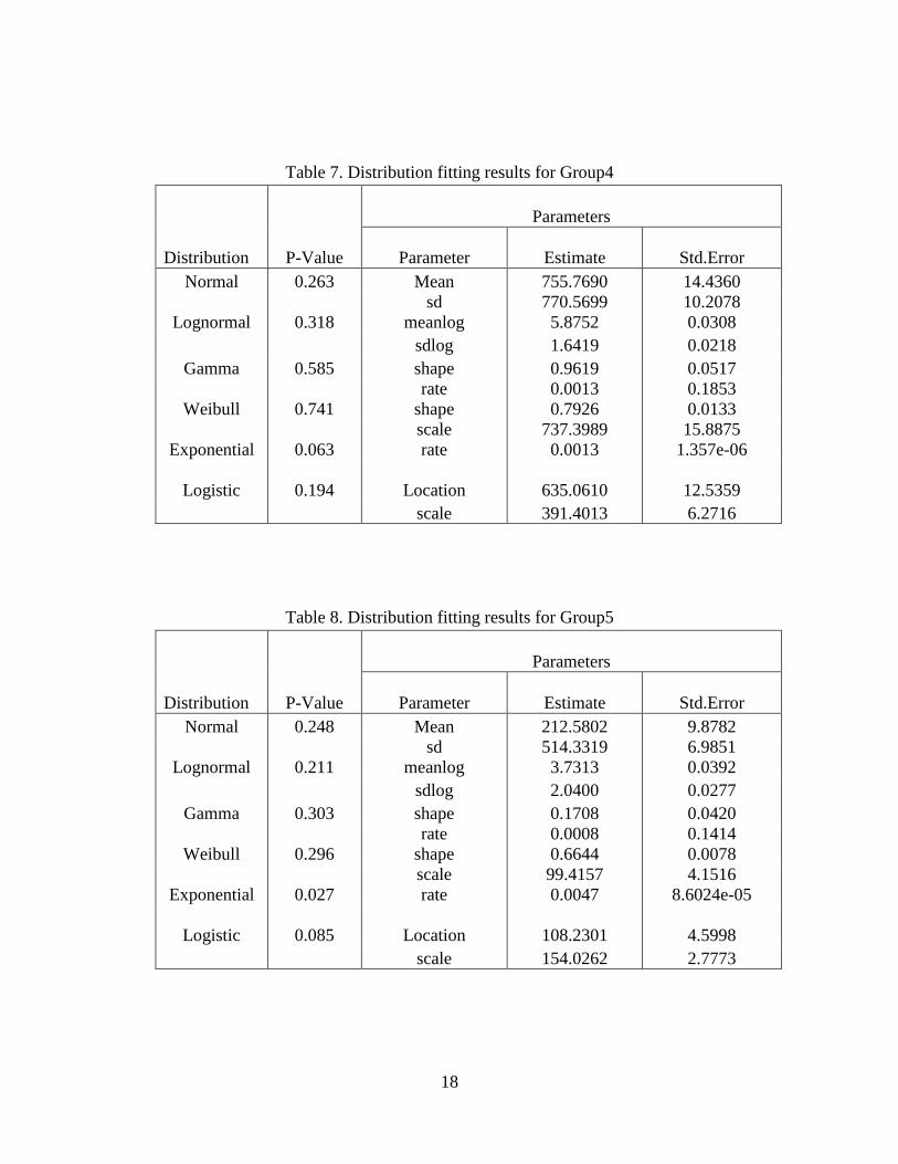
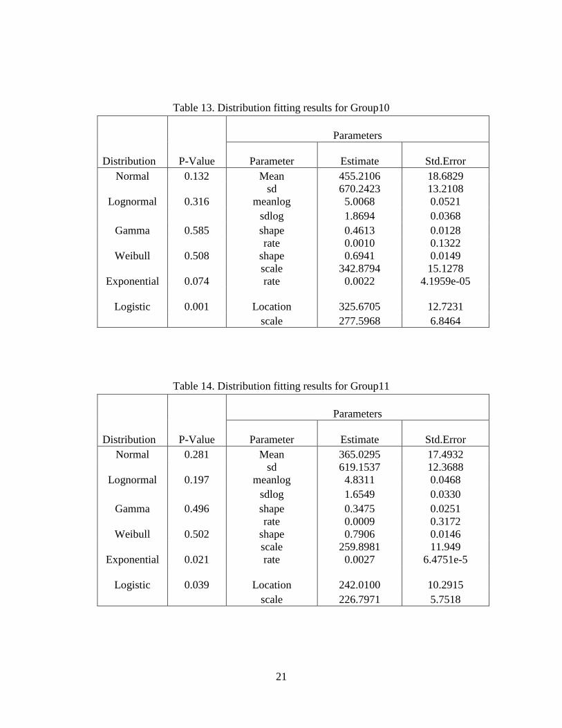
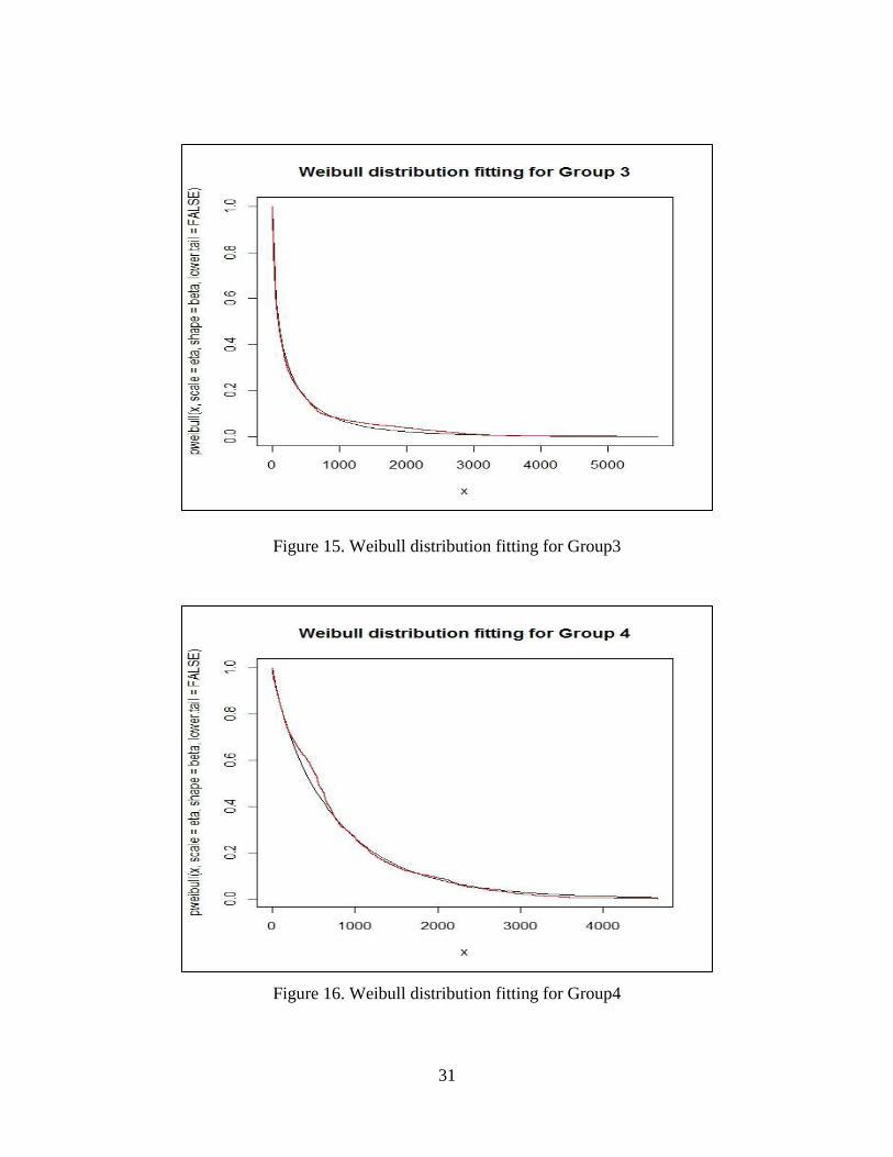
5.3 Failure time model
We assumed that the data comes from different distributions with parameters obtained by
maximum likelihood estimation and then the Kolmogorov-Smirnov test would yield p-
values. If the p-value is greater than .5 (we use .5 as the significance level), we would
decide that the data comes from this specific distribution and the distribution performs
well for the data. Table4 -Table15 give the results of the distribution fitting and
Kolmogorov-Sminrnov test for twelve groups
Table 4. Distribution fitting results for Group1
Distribution P-Value
Parameters
Parameter Estimate Std.Error
Normal 0.072 Mean 344.0772 5.2608
Lognormal
0.439
sd
meanlog
560.4689
4.7439
3.1799
0.0167
sdlog 1.7785 0.0118
Gamma 0.368 shape 0.3768 0.0321
Weibull
0.547
rate
shape
0.0011
0.7357
0.2235
0.0049
Exponential
0.131
scale
rate
251.7966
0.0029
3.7942
2.343e-5
Logistic
0.089
Location
239.4458
3.2459
scale 212.0740 1.7553
17
Table 5. Distribution fitting results for Group2
Distribution P-Value
Parameters
Parameter Estimate Std.Error
Normal 0.284 Mean 213.9361 4.0888
Lognormal
0.276
sd
meanlog
393.8215
4.3939
2.8911
0.0161
sdlog 1.5443 0.0113
Gamma 0.416 shape 0.6312 7.2257e-03
Weibull
0.322
rate
shape
0.0029
0.8681
4.2412e-05
0.0055
Exponential
0.104
scale
rate
157.4582
0.0047
2.5588
4.6174e-05
Logistic
0.128
Location
153.5818
2.3089
scale 134.1052 1.1895
Table 6. Distribution fitting results for Group3
Distribution P-Value
Parameters
Parameter Estimate Std.Error
Normal 0.375 Mean 307.5395 6.3273
Lognormal
0.371
sd
meanlog
599.2602
4.1714
4.4741
0.0219
sdlog 2.0750 0.0155
Gamma 0.438 shape 0.2634 0.0011
Weibull
0.620
rate
shape
0.0009
0.6394
0.0020
0.0045
Exponential
0.001
scale
rate
159.912
0.0033
3.5403
3.0627e-05
Logistic
0.020
Location
182.6048
3.7414
scale 220.0343 2.1125
18
Table 7. Distribution fitting results for Group4
Distribution P-Value
Parameters
Parameter Estimate Std.Error
Normal 0.263 Mean 755.7690 14.4360
Lognormal
0.318
sd
meanlog
770.5699
5.8752
10.2078
0.0308
sdlog 1.6419 0.0218
Gamma 0.585 shape 0.9619 0.0517
Weibull
0.741
rate
shape
0.0013
0.7926
0.1853
0.0133
Exponential
0.063
scale
rate
737.3989
0.0013
15.8875
1.357e-06
Logistic
0.194
Location
635.0610
12.5359
scale 391.4013 6.2716
Table 8. Distribution fitting results for Group5
Distribution P-Value
Parameters
Parameter Estimate Std.Error
Normal 0.248 Mean 212.5802 9.8782
Lognormal
0.211
sd
meanlog
514.3319
3.7313
6.9851
0.0392
sdlog 2.0400 0.0277
Gamma 0.303 shape 0.1708 0.0420
Weibull
0.296
rate
shape
0.0008
0.6644
0.1414
0.0078
Exponential
0.027
scale
rate
99.4157
0.0047
4.1516
8.6024e-05
Logistic
0.085
Location
108.2301
4.5998
scale 154.0262 2.7773

19
Table 9. Distribution fitting results for Group6
Distribution P-Value
Parameters
Parameter Estimate Std.Error
Normal 0.129 Mean 149.3701 7.5036
Lognormal
0.198
sd
meanlog
360.2581
3.4812
5.3059
0.0427
sdlog 2.0489 0.0302
Gamma 0.475 shape 0.4269 9.6851e-03
Weibull
0.462
rate
shape
0.0029
0.6651
9.2140e-05
0.0089
Exponential
0.107
scale
rate
77.3424
0.0067
3.3504
0.00014
Logistic
0.059
Location
87.1414
3.3674
scale 102.0466 1.9252
Table 10. Distribution fitting results for Group7
Distribution P-Value
Parameters
Parameter Estimate Std.Error
Normal 0.186 Mean 440.8775 14.6243
Lognormal
0.231
sd
meanlog
605.4549
5.2916
10.3409
0.0367
sdlog 1.5193 0.0259
Gamma 0.304 shape 0.5302 0.0156
Weibull
0.517
rate
shape
0.0012
0.8562
0.4725
0.0149
Exponential
0.019
scale
rate
389.5107
0.0023
12.2118
3.9407e-05
Logistic
0.006
Location
325.2677
9.4769
scale 240.5290 5.1631

20
Table 11. Distribution fitting results for Group8
Distribution P-Value
Parameters
Parameter Estimate Std.Error
Normal 0.083 Mean 362.6860 16.1953
Lognormal
0.272
sd
meanlog
597.8837
4.7626
11.4511
0.0474
sdlog 1.7495 0.0335
Gamma 0.415 shape 0.3679 0.0135
Weibull
0.658
rate
shape
0.0010
0.7475
0.1378
0.0138
Exponential
0.097
scale
rate
253.2664
0.0029
11.4421
2.343e-5
Logistic
0.020
Location
241.1684
10.0845
scale 230.3225 5.6099
Table 12. Distribution fitting results for Group9
Distribution P-Value
Parameters
Parameter Estimate Std.Error
Normal 0.133 Mean 441.9689 16.4342
Lognormal
0.208
sd
meanlog
597.1167
5.2646
11.6208
0.0443
sdlog 1.6079 0.0313
Gamma 0.457 shape 0.5479 0.2206
Weibull
0.779
rate
shape
0.0012
0.8086
0.2615
0.0171
Exponential
0.111
scale
rate
394.4956
0.0023
14.0221
4.4646e-05
Logistic
0.085
Location
335.5094
10.9036
scale 240.4056 5.8147
21
Table 13. Distribution fitting results for Group10
Distribution P-Value
Parameters
Parameter Estimate Std.Error
Normal 0.132 Mean 455.2106 18.6829
Lognormal
0.316
sd
meanlog
670.2423
5.0068
13.2108
0.0521
sdlog 1.8694 0.0368
Gamma 0.585 shape 0.4613 0.0128
Weibull
0.508
rate
shape
0.0010
0.6941
0.1322
0.0149
Exponential
0.074
scale
rate
342.8794
0.0022
15.1278
4.1959e-05
Logistic
0.001
Location
325.6705 12.7231
scale 277.5968 6.8464
Table 14. Distribution fitting results for Group11
Distribution P-Value
Parameters
Parameter Estimate Std.Error
Normal 0.281 Mean 365.0295 17.4932
Lognormal
0.197
sd
meanlog
619.1537
4.8311
12.3688
0.0468
sdlog 1.6549 0.0330
Gamma 0.496 shape 0.3475 0.0251
Weibull
0.502
rate
shape
0.0009
0.7906
0.3172
0.0146
Exponential
0.021
scale
rate
259.8981
0.0027
11.949
6.4751e-5
Logistic
0.039
Location
242.0100
10.2915
scale 226.7971 5.7518
22
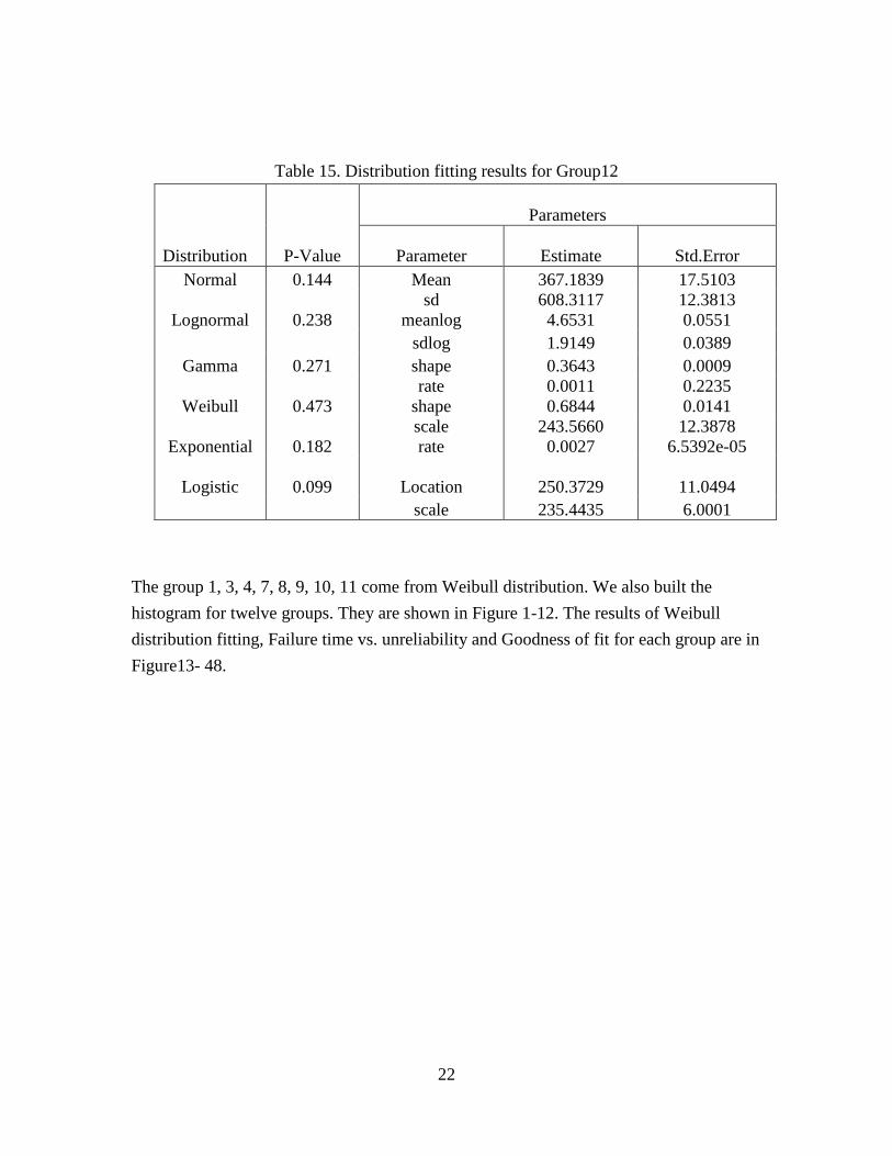
Table 15. Distribution fitting results for Group12
Distribution P-Value
Parameters
Parameter Estimate Std.Error
Normal 0.144 Mean 367.1839 17.5103
Lognormal
0.238
sd
meanlog
608.3117
4.6531
12.3813
0.0551
sdlog 1.9149 0.0389
Gamma 0.271 shape 0.3643 0.0009
Weibull
0.473
rate
shape
0.0011
0.6844
0.2235
0.0141
Exponential
0.182
scale
rate
243.5660
0.0027
12.3878
6.5392e-05
Logistic
0.099
Location
250.3729
11.0494
scale 235.4435 6.0001
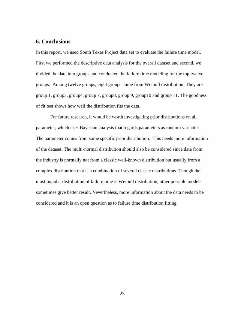
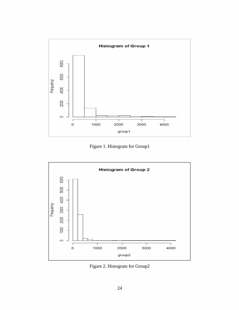
The group 1, 3, 4, 7, 8, 9, 10, 11 come from Weibull distribution. We also built the
histogram for twelve groups. They are shown in Figure 1-12. The results of Weibull
distribution fitting, Failure time vs. unreliability and Goodness of fit for each group are in
Figure13- 48.
23
6. Conclusions
In this report, we used South Texas Project data set to evaluate the failure time model.
First we performed the descriptive data analysis for the overall dataset and second, we
divided the data into groups and conducted the failure time modeling for the top twelve
groups. Among twelve groups, eight groups come from Weibull distribution. They are
group 1, group3, group4, group 7, group8, group 9, group10 and group 11. The goodness
of fit test shows how well the distribution fits the data.
For future research, it would be worth investigating prior distributions on all
parameter, which uses Bayesian analysis that regards parameters as random variables.
The parameter comes from some specific prior distribution. This needs more information
of the dataset. The multi-normal distribution should also be considered since data from
the industry is normally not from a classic well-known distribution but usually from a
complex distribution that is a combination of several classic distributions. Though the
most popular distribution of failure time is Weibull distribution, other possible models
sometimes give better result. Nevertheless, more information about the data needs to be
considered and it is an open question as to failure time distribution fitting.
24
Figure 1. Histogram for Group1
Figure 2. Histogram for Group2

25
Figure 3. Histogram for Group3
Figure 4. Histogram for Group4
26
Figure 5. Histogram for Group5
Figure 6. Histogram for Group6
27
Figure 7. Histogram for Group7
Figure 8. Histogram for Group8
28
Figure 9. Histogram for Group9
Figure 10. Histogram for Group10
29
Figure 11. Histogram for Group11
Figure 12. Histogram for Group12

30
Figure 13. Weibull distribution fitting for Group1
Figure 14. Weibull distribution fitting for Group2
31
Figure 15. Weibull distribution fitting for Group3
Figure 16. Weibull distribution fitting for Group4

32
Figure 17. Weibull distribution fitting for Group5
Figure 18. Weibull distribution fitting for Group6

33
Figure 19. Weibull distribution fitting for Group7
Figure 20. Weibull distribution fitting for Group8
34
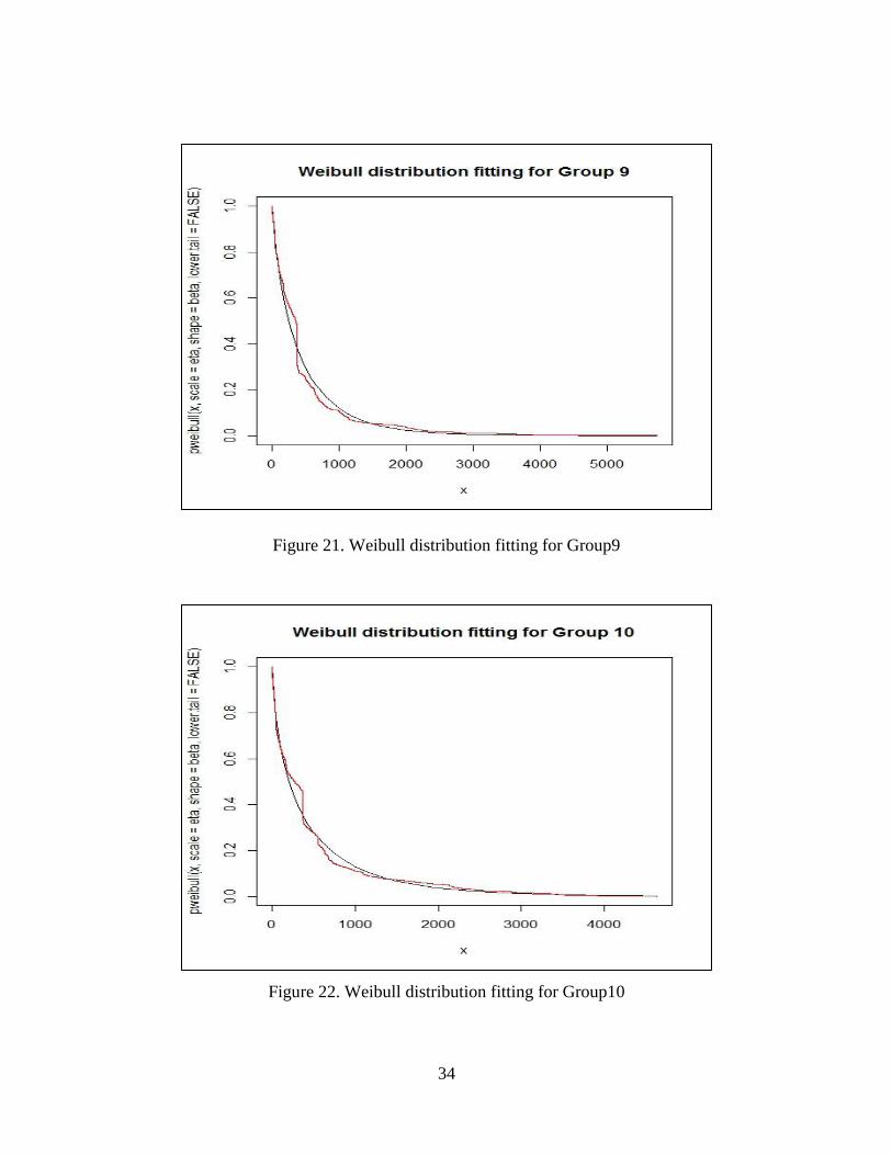
Figure 21. Weibull distribution fitting for Group9
Figure 22. Weibull distribution fitting for Group10
35
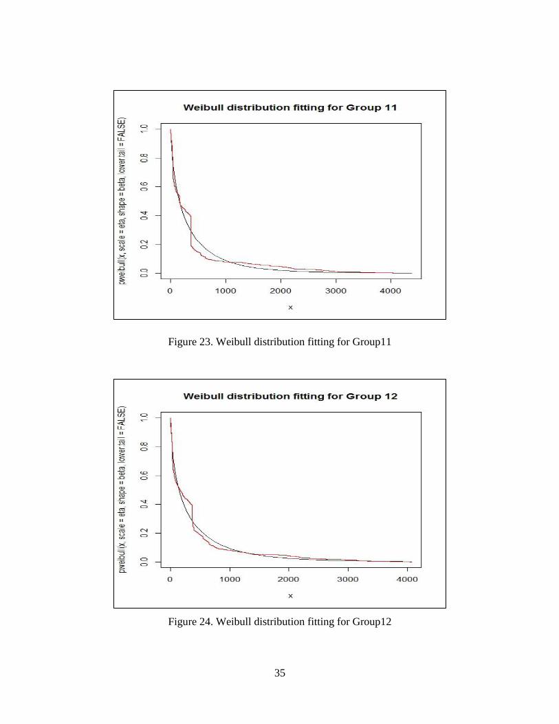
Figure 23. Weibull distribution fitting for Group11
Figure 24. Weibull distribution fitting for Group12

36
Figure 25. Failure time vs. unreliability plot for Group1
Figure 26. Failure time vs. unreliability plot for Group2
37
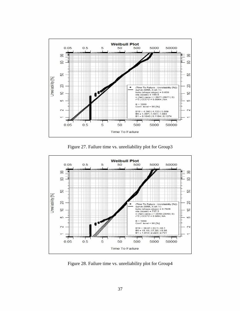
Figure 27. Failure time vs. unreliability plot for Group3
Figure 28. Failure time vs. unreliability plot for Group4
38
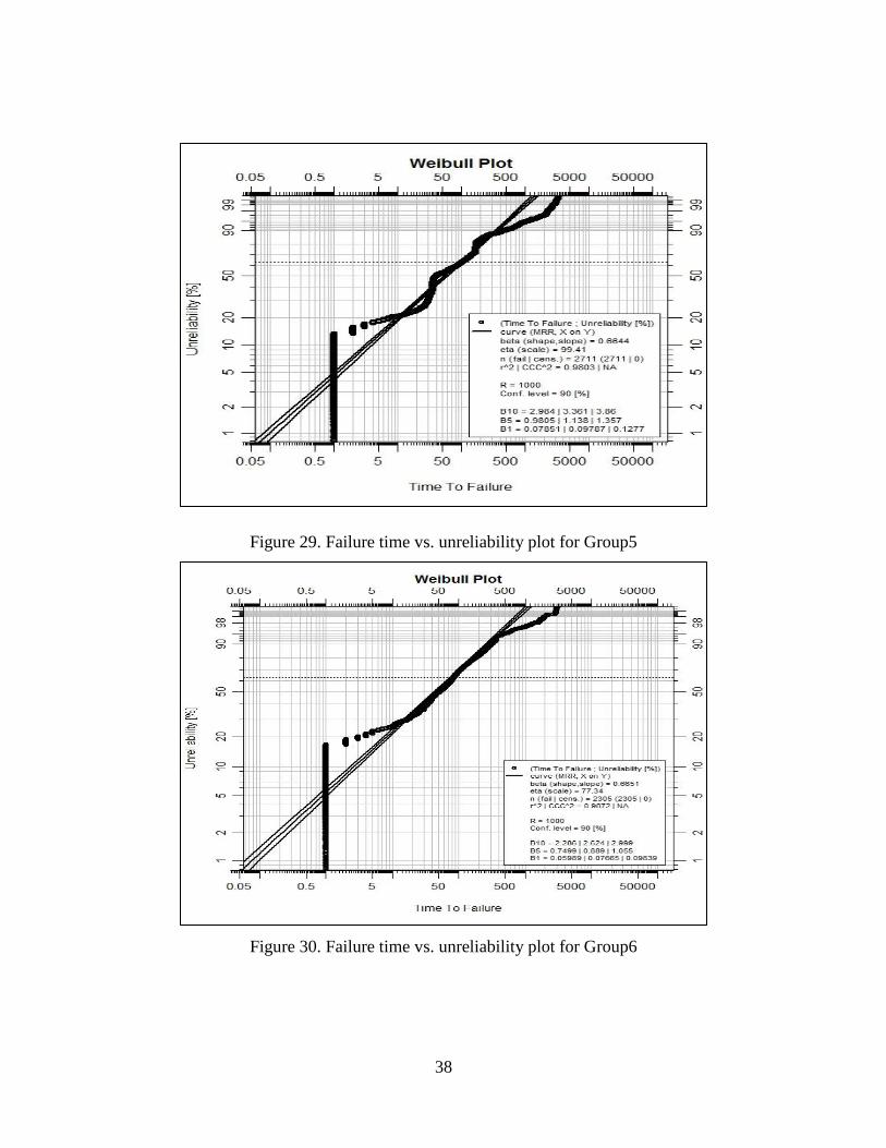
Figure 29. Failure time vs. unreliability plot for Group5
Figure 30. Failure time vs. unreliability plot for Group6

39
Figure 31. Failure time vs. unreliability plot for Group7
Figure 32. Failure time vs. unreliability plot for Group8
40
Figure 33. Failure time vs. unreliability plot for Group9
Figure 34. Failure time vs. unreliability plot for Group10
41
Figure 35. Failure time vs. unreliability plot for Group11
Figure 36. Failure time vs. unreliability plot for Group12

42
Figure 37. Weibull GOF test for Group 1
Figure 38. Weibull GOF test for Group 2

43
Figure 39. Weibull GOF test for Group 3
Figure 40. Weibull GOF test for Group 4

44
Figure 41. Weibull GOF test for Group 5
Figure 42. Weibull GOF test for Group 6

45
Figure 43. Weibull GOF test for Group 7
Figure 44. Weibull GOF test for Group 8
46
Figure 45. Weibull GOF test for Group 9
Figure 46. Weibull GOF test for Group 10
47
Figure 47. Weibull GOF test for Group 11
Figure 48. Weibull GOF test for Group 12
48
7. References
David D. Hanagal (2010). Modeling heterogeneity for bivariate survival data by the
compound Poisson distribution with random scale. Statistics and Probability, 80 (2010),
1781-1790.
Mantel, N. and Byar, D. P. (1974). Evaluation of response time data involving transient
states: an illustration using heart transplant data. J. Amer. Statist. Assoc., 69, 81-86.
Dodson Bryan(2006). The Weibull Analysis Handbook 2nd. United States: William A.
Tony.
Eckhard Limpert, Wernner A. Stahel and Markus Abbt (2001). Log-normal Distributions
across the Sciences: Keys and Clues. BioScience, 51(5), 341-351.
Knight, C.R.(1991). Four decades of reliability progress. Proceedings Annual Reliability
and Maintainability Symposium, IEEE, New York 156-159.
Joanna H. Shih and Thomas A. Louis (1995). Assessing Gamma Frailty Models for
Clustered Failure Time Data. Lifetime Data Analysis, 1, 205-220.
Patricia M. Odell, Keaven M. Anderson and Ralph B. D’s Agostino (1992). Maximum
Likelihood Estimation for Interval-Censored Data Using a Weibull Accelerated Failure
Time Model. Biometrics, 48(3), 951-959.
K.W.Fertig(1972). Bayesian prior distributions for systems with exponential failure-time
data. The Annals of Mathematical Statistics, 43(5), 1441-1448.
Peter B. Gilbert and Yanqing Sun (2005). Failure time analysis of HIV vaccine effects
on viral load and antiretroviral therapy initiation. Biostatistics, 6(3), 374-394.

49
Johnson, N.L. and Kotz, S.(1970). Distributions in Statistics: Continuous Univariate
Distributions, Boston : Houghton Mifflin.
Chi-Chao Lui (1997). A comparison between the Weibull and lognormal models used to
analyze reliability data. PhD dissertation, Graduate Program in Manufacturing
Engineering & Operations Management, The University of Nottingham, Nottingham,
UK..
In Jae Myung (2003). Tutorial on maximum likelihood estimation. Mathematical
Psychology, 47(2003), 90-100.
Werner Gurker and Reinhard Viertl(1996). Preliminary data analysis. Probability and
Statistics, Volume 2, Vienna University of Technology, Wien, Austria.
http://www.eolss.net/Sample-Chapters/C02/E6-02-04-01.pdf
Hans Riedwyl (1967). Goodness of fit. American Statistical Association, 62(318), 390-
398.
Jurgen Symynck and Filip De Bal (2011). Weibull Analysis using R in a nutshell. The
XVI-th International Scientific Conference, Stefan cel Mare University of Suceava,
Romania. http://mechanics.kahosl.be/fatimat/images/papers-books/paper-
weibull_analysis_using_r_in_a_nutshell.pdf
Leslie B. Shaffer, Timothy M. Young, Frank M. Guess, Halima Bensmail and Ramon V
(2008). Leon. Using R Software for Reliability Data Analysis. International Journal of
Reliability and Applications, 9(1), 53-70.
Willis Jackie (2005). Data Analysis and Presentation Skills: An Introduction for the Life
and Medical Sciences. United States: John Wiley & Sons, Ltd.
50
John D. Kalbfleisch and Ross L. Prentice (2011). The Statistical Analysis of Failure Time
Data. Wiley-Interscience.
Lawless, Jerald F.(1982). Statistical Models and Methods for Lifetime Data. New York:
Wiley-Interscience.
George Casella, Roger L.Berger (2001). Statistical Inference 2nd
. United States:
Thomson Learning.
Marvin Rausand and Arnljot Hoyland (2004). System reliability theory: models,
statistical methods, and applications 2nd
. United States: A John Wiley & Sons, Inc.
Wei Yu(2004). Equipment Data Development Case Study-Bayesian Weibull Analysis.
South Central SAS Users Group 14th
Annual Conference, November (7-9), 408-450.