Failure analysis of a short fibre composite bumper beam
101
Failure analysis of a short fibre composite bumper beam Physical experiments and FE-simulations Master’s Thesis in the Master’s programme of Solid and Fluid Mechanics LISA GRAUERS Department of Applied Mechanics Division of Material and Computational Mechanics CHALMERS UNIVERSITY OF TECHNOLOGY Göteborg, Sweden 2010 Master’s Thesis 2010:52
-
Upload
nguyenkhanh -
Category
Documents
-
view
224 -
download
0
Transcript of Failure analysis of a short fibre composite bumper beam
Failure analysis of a short fibre composite bumper beam
Physical experiments and FE-simulations
Master’s Thesis in the Master’s programme of Solid and Fluid Mechanics
LISA GRAUERS Department of Applied Mechanics Division of Material and Computational Mechanics
CHALMERS UNIVERSITY OF TECHNOLOGY Göteborg, Sweden 2010 Master’s Thesis 2010:52


MASTER’S THESIS 2010:52
Failure analysis of a short fibre bumper beam
Physical experiments and FE-simulations
Master’s Thesis in the Master’s programme of Solid and Fluid Mechanics
LISA GRAUERS
Department of Applied Mechanics Division of Material and Computational Mechanics
CHALMERS UNIVERSITY OF TECHNOLOGY
Göteborg, Sweden 2010

Failure analysis of a short fibre composite bumper beam Physical experiments and FE-simulations Master’s Thesis in the Master’s programme of Solid and Fluid Mechanics
LISA GRAUERS
© LISA GRAUERS, 2010
Master’s Thesis 2010:52
ISSN 1652-8557
Department of Applied Mechanics
Division of Material and Computational Mechanics
Chalmers University of Technology
SE-412 96 Göteborg
Sweden
Telephone: + 46 (0)31-772 1000
Cover: The bumper beam mounted on a car, after a crash test performed in the project where the beam was developed.
Reproservice, Chalmers Göteborg, Sweden 2010

I
Failure analysis of a short fibre composite bumper beam Physical experiments and FE-simulations Master’s Thesis in the Master’s programme of Solid and Fluid Mechanics
LISA GRAUERS Department of Applied Mechanics Division of Material and Computational Mechanics Chalmers University of Technology
ABSTRACT
A composite bumper beam in short glass fibre reinforced polyamide 6 with steel reinforcements was designed to fulfil low speed crash requirements. The first prototypes did not behave as expected according to the computer simulations and did not fulfil the requirements. Within this Master’s Thesis, the main reasons for the unsatisfactory correlation between tests and simulations are investigated. This is done by performing new experiments, which are then simulated and evaluated. The main problem with the manufactured bumper beams turned out to be the quality of the beams. The glass fibre content was much lower than expected, which gave much lower material stiffness than the one used when designing the beam. The fibre fraction did also vary from beam to beam. However, with the right properties of the material the static behaviour of the beam can be simulated with an isotropic, bilinear material model. The material was assumed to behave as an isotropic material even though the fibre orientation was not completely random. Due to the large wall thickness of the component and the relative low mould filling velocity in compression moulding, the fibres do not show a large orientation in the mould flow direction, as can normally be seen for injection moulded parts. Tests were performed in order to determine the strain rate dependence of the material. Both full scale tests on beams and tensile tests at specimens are performed. The full scale beam tests indicate a strain rate hardening of the material. In the tensile tests strain rate dependence exists for strain rates below 0.00021 s-1. The dependence above this level could not be definitely determined with the available testing equipment. The response in the dynamic crash tests can hence be assumed to be somewhat stiffer than the simulations indicate when using material properties obtained at a lower strain rate. Also, the assumed boundary conditions are shown to influence the results in the simulations of the crash tests. The simulations where simplified boundary conditions were used showed a stiffer response than when a larger part of the car was modelled. Although the fracture behaviour of the material is not fully known and it is difficult to establish a valid fracture criterion, fracture is assumed to be preceded by crazing in the polymer, which occurs at a critical strain. At the locations in the beams where fractures are expected, the strain is studied. It seems reasonable to believe that a critical strain in the range from a little less than 2 to 2.6 % is valid for the beam material. The maximum principal stresses at the fracture locations are in general lower than the measured tensile strength.
Key words: bumper beam, composite, finite element simulation, glass fibre reinforced polyamide 6, strain rate dependence, crash test

II
Contents
ABSTRACT I
CONTENTS I
PREFACE III
NOTATIONS IV
1 INTRODUCTION 1
1.1 Background 1
1.2 Aim 2
1.3 Objective 2
1.4 Limitations 2
2 METHOD 3
2.1 Parameters of interest 3
2.2 Project outline 4
2.3 Test planning 5
3 EXPLICIT FINITE ELEMENT METHOD 7
3.1 An explicit solution procedure based on the central-difference method 7
3.2 Time steps and mass scaling 8
3.3 Reduced integration and hourglass modes 9
4 SHORT GLASS FIBRE REINFORCED POLYMERS 10
4.1 Mechanics of short fibre reinforced polymers 10
4.1.1 Fracture criterions for composites and polymers 11
4.1.2 Influence from fibre length on the mechanical properties 14
4.2 Influence from manufacturing on fibre orientation 16
4.3 Influence from strain rate and temperature on the mechanical properties 17
4.4 Effects of moisture content in polyamide 19
5 EXPERIMENTS AND SIMULATIONS 20
5.1 Initial testing 20
5.1.1 Test results 21
5.1.2 Material tests 23
5.1.3 Material models 25
5.1.4 Simulations of the initial tests 28
5.1.5 Correlation between test and simulation for beam 10 28
5.1.6 Correlation between test and simulation for beam 29 32
5.2 Testing of strain rate dependence 34

II
5.2.1 Test results 34
5.2.2 Material tests and models 37
5.2.3 Simulation and correlation of the quasi static test 38
5.2.4 Simulation and correlation of the dynamic test 39
5.3 Testing with asymmetric loading 41
5.3.1 Test results 42
5.3.2 Material tests and models 43
5.3.3 Simulation and correlation of the asymmetric test 43
5.4 Testing with adhesive steel reinforcements 45
5.4.1 Test results 45
5.4.2 Material tests and models 47
5.4.3 Simulation and correlation of test 47
6 UPDATED SIMULATIONS OF PREVIOUS CRASH TESTS 50
6.1 Crash test simulations with updated material model 50
6.2 Simulation including a larger part of the car 53
7 MATERIAL SPECIFIC INVESTIGATION 55
7.1 Influence from moisture on the modulus of elasticity 55
7.2 Influence from strain rate and temperature on the modulus of elasticity 56
7.3 Material quality 59
8 RESULTS 61
9 CONCLUSIONS 63
10 DISCUSSION AND RECOMMENDATIONS 65
REFERENCES 67
APPENDIX A – MATERIAL DATA 1
APPENDIX B – LIST OF MANUFACTURED BEAMS 14
APPENDIX C – MATERIAL MODELS IN LS-DYNA 16
APPENDIX D – NOTATIONS FOR BEAM PARTS 18
APPENDIX E – UNCERTAINTIES IN SIMULATIONS AND TESTS 19
Dynamic effects in simulations of quasi static tests 19
Uncertainties concerning the testing 20
Stiffness of the rig for quasi static tests 20
Film tracking 21
Preface
This Master’s Thesis has been carried out at Epsilon UC Väst in Göteborg from March to August 2010. The Thesis is a part of a research project within FFI (Fordonsstrategisk Forskning och Innovation, Vehicle strategically research and innovation), financed by Vinnova, where Saab Automobile AB, Trollhättan and AdManus Materialteknik, Göteborg have been involved together with Epsilon.
I would like to thank my supervisor, Johan Iraeus, Epsilon, and examiner, Mats Ander, the Department of Applied Mechanics at Chalmers University of Technology in Göteborg, for interesting discussions and valuable inputs as well as support and encouragement throughout the project. I would also like to thank Anders Sjögren, AdManus Materialteknik, for an interesting work with the material testing. At last, I would like to thank Fredrik Svensson, Claes Ljungqvist and Louise Lindell at Saab Automobile AB, for their work within the research project and Vitomir Penava for his help in the low speed crash test laboratory at Saab Automobile AB.
Göteborg, August 2010
Lisa Grauers
IV
Notations
Explanation of the notation used in the report, presented in order of appearance. A few notations appear more than once but it should be clear from the context which one is intended.
M The mass matrix
C The damping matrix K The stiffness matrix
nextR , The external forces at time step n
nd The nodal displacements at time step n
nd& The nodal velocities at time step n
nd&& The nodal accelerations at time step n
nd&&& The third time derivative on the nodal displacement at time step n
t∆ The length of the time step L The shortest characteristic length of an element
c The acoustic wave speed
ρ The material density
1σ Stress in the fibre direction in a composite lamella
2σ Stress in the transverse fibre direction in a lamella
12τ Shear stress in a lamella
xσ Stress in the x-direction, similar notation for y- and z-direction
xyτ Shear stress in the xy-plane, similar notation for yz- and xz-plane
cl Critical fibre length
d Fibre diameter *
fσ Ultimate strength of a fibre
cτ The fibre-matrix bond strength
E Modulus of elasticity
1E Modulus of elasticity in the fibre direction of a lamella with continuous
fibres
2E Modulus of elasticity in the transverse fibre direction of a lamella with
continuous fibres
fE Modulus of elasticity of the fibre
mE Modulus of elasticity of the matrix
fV Volume fraction fibres
mV Volume fraction matrix
1E Modulus of elasticity in the fibre direction of a lamella with the same fibre fraction but parallel fibres, used for random oriented lamellas
2E Modulus of elasticity in the transverse fibre direction of a lamella with the same fibre fraction but parallel fibres, used for random oriented lamellas
ranE Modulus of elasticity of a random oriented short fibre composite
K Efficiency parameter for short fibres

extE ,1 Modulus of elasticity, tested at 1 mm/min, strain measured with
extensometer
5E Modulus of elasticity, tested at 5 mm/min, strain measured between the
grips
tanE Tangent modulus
5tan,E Tangent modulus, tested at 5 mm/min, strain measured between the grips
5,uσ Ultimate stress, tested at 5 mm/min
yσ Yield stress
5,fε Strain at fracture, tested at 5 mm/min, strain measured between the grips
GF Weight fraction glass fibre
1ε Maximum principal strain
modε Modified principal strain

VI

CHALMERS, Applied Mechanics, Master’s Thesis 2010:52 1
1 Introduction
1.1 Background
The background for this Master’s Thesis is a project where a new front bumper beam concept for a Saab 9-3 Convertible was developed. In order to reduce the weight, a beam in short fibre composite was requested. The new concept had to fulfil the same crash requirements and be equivalent to the prior steel concept. The beam was simulated with the FE-software LS-DYNA and designed virtually in order to fulfil the requirements of the crash test CMVSS2151.
However, when physical tests on the first prototypes were performed the beam did not fulfil the requirements. The results in the simulations and tests did not correlate since the response in the simulations was stiffer than in the actual tests and failure did occur at lower stress levels than expected. A new project, financed by Vinnova, to deepen the knowledge about short fibre composite materials was initiated. The aim is to gain the future use of these materials in a wider range of components subjected to load. That is for example relevant in the car industry. Compression moulding was chosen for manufacturing the beam, since it is a cheap and efficient way to produce large series of components in short fibre composite. It is also of interest to achieve more knowledge about the fibre orientation and the material quality obtained with this manufacturing method. This Master’s Thesis is a part of this bigger Vinnova-project.
The bumper beam is made of short glass fibre reinforced polyamide 6. The beam is reinforced with steel on both front and rear side, as shown in Figure 1. The steel is a HyTens 1200 stainless steel with a high yield stress to reduce the residual deformation after the CMVSS215 pendulum impacts. It has also a relatively high ultimate strain in order to ensure certain ductility, where the steel is subjected to high tensile stresses. The steel reinforcements are bonded to the beam with the epoxy based structural adhesive Terokal 50872, which has been developed for bonding in the automotive industry. The adhesive has high peel and impact peel resistance.
Figure 1. The steel reinforcements on the front and rear side of the bumper beam.
In front of the beam with its steel reinforcements, a bumper beam foam is placed, see Figure 2, to distribute the load from an impact. The beam is fastened to the frame of
1 CMVSS215 are Canadian legislation, low speed, crash tests which include high and low pendulum impacts (8 km/h), corner pendulum impact (5 km/h) and a fixed-barrier collision (8 km/h). 2 The adhesive Terokal 5087 is today replaced by Terokal 5089, which should have equivalent properties.

CHALMERS, Applied Mechanics, Master’s Thesis 2010:52 2
the car with bolts through the crash boxes. The bolts are supposed to tear through the crash boxes and thereby absorb energy in certain crash situations. The notation used for parts of the beam is clarified in Appendix D.
Figure 2. The bumper foam in front of the bumper beam.
1.2 Aim
The main purpose is to gain more knowledge about simulations of the behaviour of short fibre composites, which is important for future use of these materials. In many fields today, lightweight construction is of big interest and due to the short development times, the main part of the design process is done with simulations. Therefore trustworthy simulations even for short fibre composites are very important.
1.3 Objective
The objective of this Master’s Thesis is to investigate why the crash tests and the simulations for the bumper beam did not correlate in the previous project. Parameters influencing the correlation will be identified and studied in order investigate how the simulations can be improved to give a better prediction of the real behaviour of short fibre composites.
1.4 Limitations
Due to the limited time and the complexity of the project, all parameters influencing the correlation can not be investigated. The main focus is a comprehensive investigation including the parameters that are considered to be most important, rather than to go through all the possible parameters in the beam concept. Implementation of all the gained results in new, improved simulations of the prior crash tests will not be included. For the experiments within the Master’s Thesis, there are only a limited number of beams available. There is no possibility to produce new beams or pieces of equivalent material. Equipment for high strain rate tensile testing of material properties is not available within the project.
CHALMERS, Applied Mechanics, Master’s Thesis 2010:52 3
2 Method
In order to investigate why the correlation between the crash tests and the corresponding FE-simulations in the previous project was unsatisfactory, parameters of interest are identified. The aim is to perform tests were the influence from different parameters could be determined. In this section the most important parameters likely to affect the correlation are presented, followed by a basic project outline. Finally, the given conditions, from which the tests are planned and performed, are described. These conditions are included in this section since they strongly affect the method chosen for the work in this project.
2.1 Parameters of interest
The correlation between the actual tests and the simulations is dependent on a large number of parameters. Important parameters are identified on the basis of experience from the prior project and by studying relevant literature. The following parameters are identified as likely to cause correlation problems:
• Fibre orientation and fibre fraction
• Quality of the material o Adhesion between fibres and matrix o Moisture content o Pores and other defects o Heat degradation
• Strain rate dependence
• Adhesive joints between the beam and the steel reinforcements
• Boundary conditions, including bolts and the bumper beam foam
These parameters might in different ways influence the behaviour of the beam and are briefly described below. The mechanical properties of short fibre composite materials are dependent on fibre fraction and fibre orientation. In the simulations of the crash tests in the previous project, the assumption of isotropic material was made. This is however doubtful, since the manufacturing may lead to an uneven fibre distribution and orientation.
The quality of the material is also very important for the performance of the beam. In order to take advantage of the properties of the different phases of a composite, the adhesion between the matrix and the fibres must be good. The matrix material in the beam is polyamide 63, which is sensitive to moisture. The moisture affects the mechanical properties of the material in the same ways as a softener. Pores in the material also affect the properties. Reasons for degradation of the material can be ageing or exposure to high temperatures or UV-light, (Klason, Kubát, 2004). Here especially high temperatures can be relevant since the beam is exposed to temperatures around 200 ˚C during the curing of the adhesive.
3 Ultramid® B3S, Polyamide 6.

CHALMERS, Applied Mechanics, Master’s Thesis 2010:52 4
The behaviour of polymers is dependent on both strain rate and temperature. The material testing for the beam material in the previous project was performed at two different strain rates. Both are much smaller than the actual strain rate in the crash tests and the large variation in the test results made it impossible to draw any conclusion concerning the strain rate dependence. At higher strain rates the polymer generally acts stiffer. The same trend is the case when the temperature is lowered, (Klason, Kubát, 2004).
The beam steel reinforcements are fastened through adhesive joints. To reach the optimal performance the adhesive joints are of big importance. The adhesive must be able to undergo the crash loadings with neither adhesive nor cohesive fractures, since that would change the dynamic properties of the beam drastically. The adhesive joints must also be simulated in a proper way. The adhesive should be applied in a thin, even layer in order to achieve the defined properties. When producing the beam, the adhesive was distributed by hand and the quality and accuracy is not assured.
In the simulations, the ends of the bolts between the crash boxes and the side beams were assumed to be fixed. The side beams and rest of the car was neglected. It may be relevant to see how this simplification and other types of boundary conditions affect the performance of the beam in the simulations. Other parts of the car are also available for simulations and including a larger part of the car might improve the correlation. The used type of bumper beam foam has caused a somewhat stiffer response in simulations compared to actual crash tests in other projects.
2.2 Project outline
The tests are designed in such a way that the influence from different parameters can be identified. Initially, the validity of the assumption of isotropic material is investigated, with the other parameters eliminated. The correlation between these initial tests and simulations will determine the continued work within the project. In case of bad correlation, the properties of the material in the tested beams must be investigated more in detail. That includes fibre orientation and fibre fraction in different parts of the beam. Most likely an anisotropic material model must be used in this case. If the correlation after the initial testing is sufficient, the assumption of isotropic material will be considered accurate enough. The next step will then be to study the influence from the other described parameters. Individual parameters or groups of parameters will be included in order to draw conclusions about their significance for the correlation between tests and simulations. A principal illustration of the work process can be seen in Figure 3.
The tests are done in different batches, since the outcome of the performed tests and the corresponding simulations determine which tests that would be relevant to continue with. Therefore, new tests are designed after the evaluation of the previous ones. The properties of the material in each beam are determined at AdManus Materialteknik after the tests, in order to be able to use more accurate material models in the simulations.

CHALMERS, Applied Mechanics, Master’s Thesis 2010:52 5
Figure 3. A principal illustration of the work process within the project. Experiments
including different parameters will be performed. Whether the
correlation is good or bad will determine the continued path.
In order to make the work process clearer and easier to track, it is presented in a chronological order in this report. The basic structure for the work can be seen in Figure 4. First, a presentation and motivation of the test set up, followed by the test results are described. After that, the results from the testing performed on the beam material are presented along with the material model for the simulation of the test. Next, the simulation of the test is described and finally, the correlation between the test and the simulation is evaluated. This procedure will be looped through for each batch of tests. The complete work process is presented in Section 5. During the project, some parameters required further investigation or additional simulations. These parts of the project are presented in Section 6 and 7, after the above described work process, even though they were performed parallel. In Section 8, a summary of the obtained results are presented, followed by the drawn conclusions in Section 9 and a discussion with recommendations for future work in Section 10.
Figure 4. The basic loop for the work presented in Section 5.
The work within the project is connected to and based on theory obtained from literature on the topics. The basic theory for the explicit finite element method can be found in Section 3. Theory on short fibre reinforced polymers and polyamide are presented in Section 4.
2.3 Test planning
The physical tests are planned on the basis of the given conditions in terms of number of beam prototypes and the crash test equipment at Saab Automobile AB, Trollhättan,
CHALMERS, Applied Mechanics, Master’s Thesis 2010:52 6
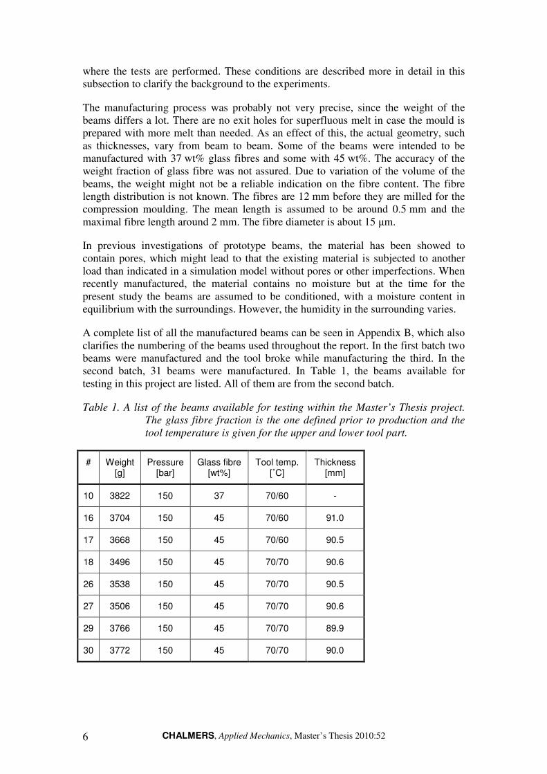
where the tests are performed. These conditions are described more in detail in this subsection to clarify the background to the experiments.
The manufacturing process was probably not very precise, since the weight of the beams differs a lot. There are no exit holes for superfluous melt in case the mould is prepared with more melt than needed. As an effect of this, the actual geometry, such as thicknesses, vary from beam to beam. Some of the beams were intended to be manufactured with 37 wt% glass fibres and some with 45 wt%. The accuracy of the weight fraction of glass fibre was not assured. Due to variation of the volume of the beams, the weight might not be a reliable indication on the fibre content. The fibre length distribution is not known. The fibres are 12 mm before they are milled for the compression moulding. The mean length is assumed to be around 0.5 mm and the maximal fibre length around 2 mm. The fibre diameter is about 15 µm.
In previous investigations of prototype beams, the material has been showed to contain pores, which might lead to that the existing material is subjected to another load than indicated in a simulation model without pores or other imperfections. When recently manufactured, the material contains no moisture but at the time for the present study the beams are assumed to be conditioned, with a moisture content in equilibrium with the surroundings. However, the humidity in the surrounding varies.
A complete list of all the manufactured beams can be seen in Appendix B, which also clarifies the numbering of the beams used throughout the report. In the first batch two beams were manufactured and the tool broke while manufacturing the third. In the second batch, 31 beams were manufactured. In Table 1, the beams available for testing in this project are listed. All of them are from the second batch.
Table 1. A list of the beams available for testing within the Master’s Thesis project.
The glass fibre fraction is the one defined prior to production and the
tool temperature is given for the upper and lower tool part.
# Weight [g]
Pressure [bar]
Glass fibre [wt%]
Tool temp. [˚C]
Thickness [mm]
10 3822 150 37 70/60 -
16 3704 150 45 70/60 91.0
17 3668 150 45 70/60 90.5
18 3496 150 45 70/70 90.6
26 3538 150 45 70/70 90.5
27 3506 150 45 70/70 90.6
29 3766 150 45 70/70 89.9
30 3772 150 45 70/70 90.0

CHALMERS, Applied Mechanics, Master’s Thesis 2010:52 7
3 Explicit finite element method
The finite element procedures used in structural dynamics can be divided into implicit and explicit methods. Normally, the implicit methods are used for structural applications with a low-frequency response and the explicit for wave propagation and impact problems, (Crisfield, 1997). The simulations throughout the project are performed with the explicit finite element method software LS-DYNA. Some basics concerning explicit finite element methods are described in this section.
3.1 An explicit solution procedure based on the central-
difference method
The central-difference method is presented as a basis for the time-integration in LS-DYNA. It is a method which is frequently used and characteristic for explicit methods in general, (Cook et al., 1989). It will be described in this subsection. The equation of motion for a specific time, n, is written as
nextnnn RKddCdM ,=++ &&& (3.1)
where M is the mass matrix, C the damping matrix, K the stiffness matrix, nextR , the
external forces, nd the nodal displacements, nd& the nodal velocities and nd&& the nodal
accelerations.
The nodal displacements dn+1 and dn-1 are expanded in Taylor series around the present time as follows
⋅⋅⋅+∆
+∆
+∆+=+ nnnn dt
dt
dtdd &&&&&&
62
32
1 (3.2)
⋅⋅⋅+∆
−∆
+∆−=− nnnn dt
dt
dtdd &&&&&&
62
32
1 (3.3)
By subtracting Equation (3.3) from (3.2), the velocities are obtained as
( )112
1−+ −
∆= nnn dd
td& (3.4)
And by adding Equation (3.2) and (3.3), the accelerations are obtained as
( )1122
1−+ +−
∆= nnnn ddd
td&& (3.5)
Terms containing 2t∆ or higher are excluded, which makes the central-difference second order accurate, i.e. the error is quartered if the time step is halved.

CHALMERS, Applied Mechanics, Master’s Thesis 2010:52 8
When Equation (3.4) and (3.5) are used in (3.1), it results in
( ) 112,12 2
12
1
2
11−−+
∆+−
∆+−=
∆+
∆nnnnnextn Cd
tddM
tKdRdC
tM
t (3.6)
From this system of equations, the accelerations can be calculated. As stated in the previous subsection, the equations are uncoupled if M and C are diagonal. There are alternative forms of the central-difference method that do not require a diagonal form of C. One example is by lagging the velocity in Equation (3.1) by one half time step, i.e. dn is replaced dn-1/2, (Cook et al., 1989).
3.2 Time steps and mass scaling
Explicit methods are in general conditionally stable and if the time step is too large, the method will be unstable. On the other hand, if the time step is very small the computations will be too expensive, (Cook et al., 1989). Based on this, a time step of appropriate length must be determined. The maximum time step roughly corresponds to the time it takes an acoustic wave to pass through an element, using the shortest characteristic length. With L denoting this length and c denoting the acoustic wave speed, the time step can be determined as
c
Lt ≤∆ (3.7)
which is called the CFL condition after Courant, Friedrichs and Lewy. The physical interpretation of this condition is that the time step must be so small in order for the information not to travel more than one element during each time step. The elements will be looped through to find the minimum required time step, (Cook et al., 1989). A scale factor for the time step can be used in order to ensure the stability and the default value of this factor in LS-DYNA is 0.9, (Hallquist, 2006).
When a model includes elements with a small shortest characteristic length, the required time step will be very small. The wave speed through a material can be determined as
ρ
Ec = (3.8)
By increasing the density of the material, the time it takes for the acoustic wave to pass will increase due to the lowered wave speed. The density is increased in the critical elements and therefore the time step can be kept quite large without getting instability, (Cook et al., 1989). When a mass scaled solution is used, a shortest allowed time step is defined and mass will be added to the elements not fulfilling this time step until they do, (LS-DYNA Keyword User’s Manual, Version 971, Volume I, 2007). The added mass should be small compared to the mass of the simulated part to not affect the results.
CHALMERS, Applied Mechanics, Master’s Thesis 2010:52 9
3.3 Reduced integration and hourglass modes
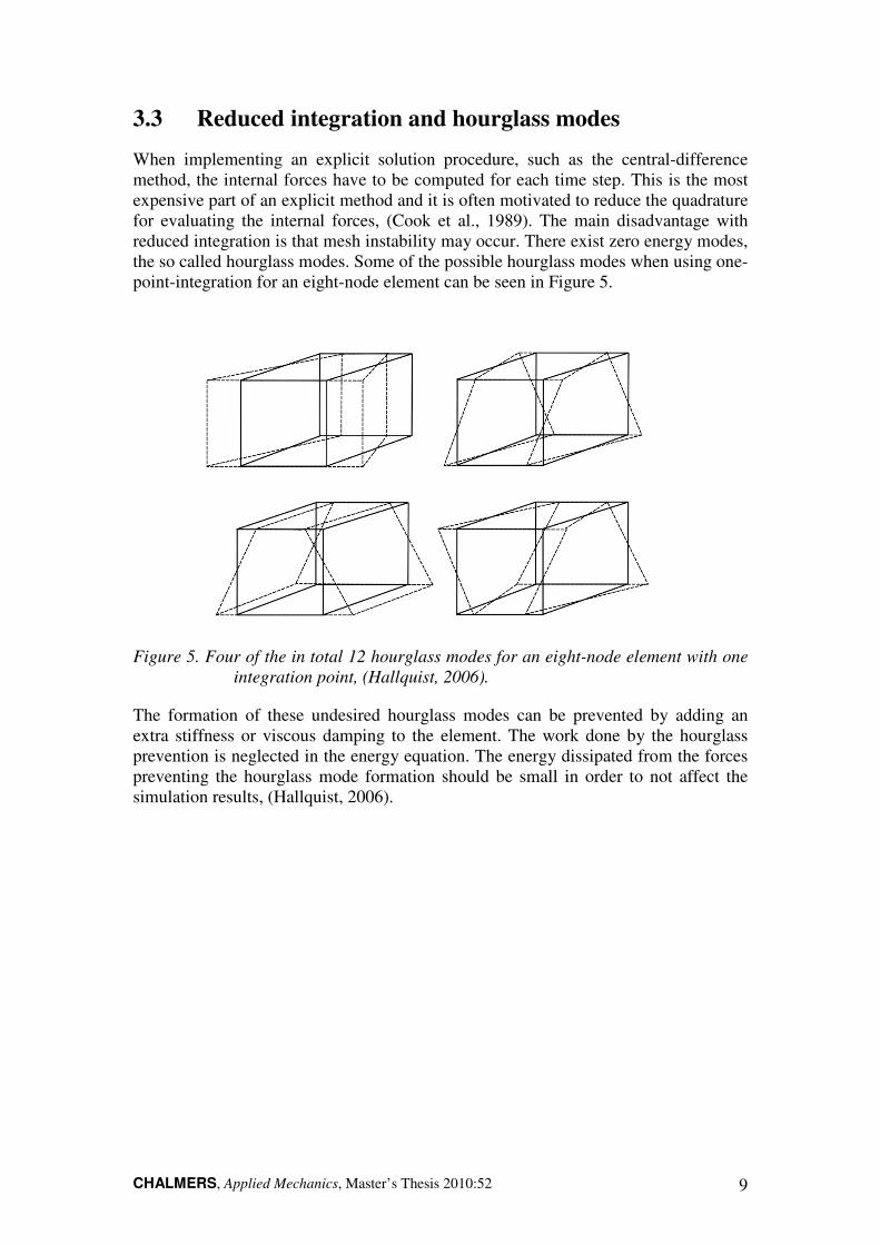
When implementing an explicit solution procedure, such as the central-difference method, the internal forces have to be computed for each time step. This is the most expensive part of an explicit method and it is often motivated to reduce the quadrature for evaluating the internal forces, (Cook et al., 1989). The main disadvantage with reduced integration is that mesh instability may occur. There exist zero energy modes, the so called hourglass modes. Some of the possible hourglass modes when using one-point-integration for an eight-node element can be seen in Figure 5.
Figure 5. Four of the in total 12 hourglass modes for an eight-node element with one
integration point, (Hallquist, 2006).
The formation of these undesired hourglass modes can be prevented by adding an extra stiffness or viscous damping to the element. The work done by the hourglass prevention is neglected in the energy equation. The energy dissipated from the forces preventing the hourglass mode formation should be small in order to not affect the simulation results, (Hallquist, 2006).

CHALMERS, Applied Mechanics, Master’s Thesis 2010:52 10
4 Short glass fibre reinforced polymers
The bumper beam is made of short glass fibre reinforced polyamide 6, PA6. Both composite materials and polymers are materials that differ quite a lot from the metals normally used in these applications. This requires knowledge and extra attention to the loading that the material is subjected to. In this section the mechanical properties of short fibre reinforced polymers as well as more specific properties for polyamide are described. Values for some properties for neat PA6 of the type used in the beam and typical E-glass fibres can be found in Appendix A, Table A. 7 and Table A. 8.
4.1 Mechanics of short fibre reinforced polymers
In the mechanics of short fibre composites, the fibres and the matrix can not be assumed to be subjected to the same strain, as usually done for continuous fibre composites. In this case, the matrix will normally be more elongated than the fibres. Due to the difference in elongation a shear stress will build up in the interface between the matrix and the fibres. The shear stress will transfer the load from the matrix to the fibres, (Piggott, 2002). Since the matrix will transfer the load from one fibre to another adjacent one, the fibre-matrix and the fibre-fibre interactions are very important in short fibre composites, (Kelly, Zweben, 2000). One way to describe the load transfer, within the classical elasticity theory, is the single fibre model. A single fibre embedded in matrix is studied, see Figure 6. When a load is applied to the piece of material, the load will be transferred from the matrix to the fibre in the matrix-fibre interface, (Kelly, Zweben, 2000).
Figure 6. The single fibre model subjected to the force F, (Kelly, Zweben, 2000).
Already in year 1952, Cox developed a theory concerning the complex interactions between fibres and matrix in short fibre composites, a shear-lag theory. The shear stress is largest at the ends of the fibre. The normal tensile stress in the fibre is zero at the ends, but will build up and reach its maximum in the middle, see Figure 7. According to Cox’ analysis the shear stress near the fibre ends will quickly rise to values which can exceed the strength of the matrix material, with shear failure at the interface as consequence. This would happen prior to fibre failure due to its critical stress. Because of this, the Cox theory is mostly used in estimations of the modulus of elasticity. The theory is still considered to be simple and adequate. The shear lag

CHALMERS, Applied Mechanics, Master’s Thesis 2010:52 11
theory has been subject for refinements, but most of them have included a lot of complexity, without a lot of further improvement in the predictions, (Piggott, 2002).
Figure 7. The distribution of the tensile stress in the fibre and the shear stress in the
interface along the fibre of length L, (Kelly, Zweben, 2000).
The strength of a short fibre composite has instead been approximated with a completely different approach. The strength has been assumed to depend on yielding and/or frictional slip at the interface between the matrix and the fibres. Early made investigations seemed to support this assumption, but further tests with short glass and carbon fibres did not show the same behaviour, expect when special silicon coatings were used on the fibres, (Piggott, 2002).
4.1.1 Fracture criterions for composites and polymers
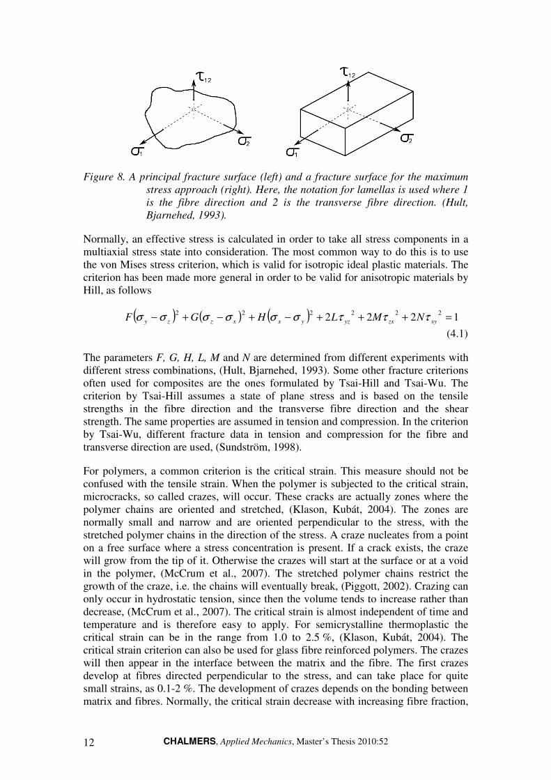
When material data for fracture are determined in experiments, it is normally done in tensile tests where specimens are loaded in one direction. This uniaxial stress state is normally not present in the real component when loaded in use. To predict where fracture occurs, methods for how fractures in multiaxial stress states can be determined from the uniaxial fracture data from experiments are needed. There are different approaches to obtain this. First, an empirical model, which is directly adjusted, can be used. Second, a fracture mechanical model can be used. In an empirical model established from tests, the results can be geometrically shown in fracture surfaces, see Figure 8. A stress state is represented by a point in the stress state and as long as this point is situated inside the fracture surfaces, fracture will not occur, (Hult, Bjarnehed, 1993).
In the maximum stress approach, fracture is assumed to occur when one of the stress components reach its fracture value, determined from experiments. These fracture surfaces are plane and build a parallelepiped, see Figure 8. The stress components are assumed to be independent from each other, which normally leads to an overestimation of the load the material can stand. Another approach is to use the maximum strains, corresponding to the maximum stresses, as the criteria for fracture, as for brittle materials. These strains are measured in experiments. If the material behaviour is linear elastic until fracture, the fracture surfaces build a polyhedron, (Hult, Bjarnehed, 1993).
CHALMERS, Applied Mechanics, Master’s Thesis 2010:52 12
Figure 8. A principal fracture surface (left) and a fracture surface for the maximum
stress approach (right). Here, the notation for lamellas is used where 1
is the fibre direction and 2 is the transverse fibre direction. (Hult,
Bjarnehed, 1993).
Normally, an effective stress is calculated in order to take all stress components in a multiaxial stress state into consideration. The most common way to do this is to use the von Mises stress criterion, which is valid for isotropic ideal plastic materials. The criterion has been made more general in order to be valid for anisotropic materials by Hill, as follows
( ) ( ) ( ) 1222222222
=+++−+−+− xyzxyzyxxzzy NMLHGF τττσσσσσσ
(4.1)
The parameters F, G, H, L, M and N are determined from different experiments with different stress combinations, (Hult, Bjarnehed, 1993). Some other fracture criterions often used for composites are the ones formulated by Tsai-Hill and Tsai-Wu. The criterion by Tsai-Hill assumes a state of plane stress and is based on the tensile strengths in the fibre direction and the transverse fibre direction and the shear strength. The same properties are assumed in tension and compression. In the criterion by Tsai-Wu, different fracture data in tension and compression for the fibre and transverse direction are used, (Sundström, 1998).
For polymers, a common criterion is the critical strain. This measure should not be confused with the tensile strain. When the polymer is subjected to the critical strain, microcracks, so called crazes, will occur. These cracks are actually zones where the polymer chains are oriented and stretched, (Klason, Kubát, 2004). The zones are normally small and narrow and are oriented perpendicular to the stress, with the stretched polymer chains in the direction of the stress. A craze nucleates from a point on a free surface where a stress concentration is present. If a crack exists, the craze will grow from the tip of it. Otherwise the crazes will start at the surface or at a void in the polymer, (McCrum et al., 2007). The stretched polymer chains restrict the growth of the craze, i.e. the chains will eventually break, (Piggott, 2002). Crazing can only occur in hydrostatic tension, since then the volume tends to increase rather than decrease, (McCrum et al., 2007). The critical strain is almost independent of time and temperature and is therefore easy to apply. For semicrystalline thermoplastic the critical strain can be in the range from 1.0 to 2.5 %, (Klason, Kubát, 2004). The critical strain criterion can also be used for glass fibre reinforced polymers. The crazes will then appear in the interface between the matrix and the fibre. The first crazes develop at fibres directed perpendicular to the stress, and can take place for quite small strains, as 0.1-2 %. The development of crazes depends on the bonding between matrix and fibres. Normally, the critical strain decrease with increasing fibre fraction,

CHALMERS, Applied Mechanics, Master’s Thesis 2010:52 13
(Klason, Kubát, 2004). The fractures in tensile tests performed on neat polyamide 664, PA66, and short glass fibre reinforced PA66 has been studied, (Mohimid et al., 2006). The neat PA66 showed crazing prior to fracture, but in the reinforced PA66 the reason to fracture instead seemed to be fibre-matrix interface rupture and fibre pull out.
The first sign of an upcoming failure in a ductile material is normally yielding. The shear yield stress can be estimated if the uniaxial yield stress in tension and compression is known. The yield stress is normally not the same in tension and compression for polymers. The end of the failure process is the separation into two parts. For polymers, yielding and/or crazing usually precede this. Simple compression is not likely to cause failure, if not the material is very brittle. Fracture should be possible in both shear and tension, but shear fractures are rather rare. There is a widely used shear test for composites, named after its inventor N. Iosipescu. For neat polymers tested in this shear test, shear failure does not occur. When thinking of polymers as being long polymer chains, the response in shear and tension has the same end result, see Figure 9. For the shortest polymer chains, another approach will be needed since it is a question of them being pulled out rather than straightened and fractured, (Piggott, 2002).
Figure 9. Large tensile (top) and shear (bottom) deformations of polymers modelled
as chains, (Piggott, 2002).
For short fibre reinforced polymers, the failure mode is dependent on both the load and the material configuration, i.e. the type and the efficiency of the reinforcements, (De Monte et al., 2009). Several different fracture mechanisms can occur and a fracture analysis is needed in order to understand the fracture. After being loaded further than the so called loosening point, approximately a quarter of the ultimate strength, the composite is assumed to contain many small cracks at the fibre ends. As a crack develops in the material, the location of fibres in its way will contribute to the breaking force in different ways. The mechanisms can be explained by studying a
4 The main differences between polyamide 6 and polyamide 66 are that polyamide 66 is more heat resistant and absorbs less moisture. Polyamide 66 can also be written polyamide 6.6.
CHALMERS, Applied Mechanics, Master’s Thesis 2010:52 14
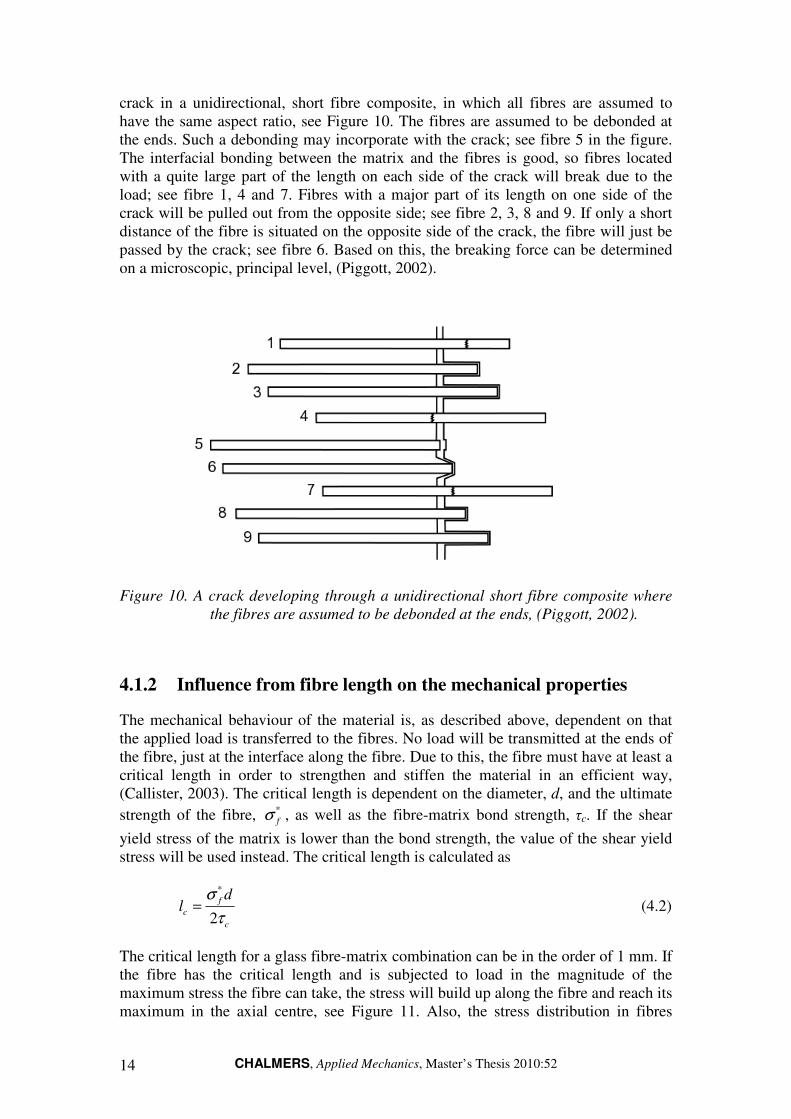
crack in a unidirectional, short fibre composite, in which all fibres are assumed to have the same aspect ratio, see Figure 10. The fibres are assumed to be debonded at the ends. Such a debonding may incorporate with the crack; see fibre 5 in the figure. The interfacial bonding between the matrix and the fibres is good, so fibres located with a quite large part of the length on each side of the crack will break due to the load; see fibre 1, 4 and 7. Fibres with a major part of its length on one side of the crack will be pulled out from the opposite side; see fibre 2, 3, 8 and 9. If only a short distance of the fibre is situated on the opposite side of the crack, the fibre will just be passed by the crack; see fibre 6. Based on this, the breaking force can be determined on a microscopic, principal level, (Piggott, 2002).
Figure 10. A crack developing through a unidirectional short fibre composite where
the fibres are assumed to be debonded at the ends, (Piggott, 2002).
4.1.2 Influence from fibre length on the mechanical properties
The mechanical behaviour of the material is, as described above, dependent on that the applied load is transferred to the fibres. No load will be transmitted at the ends of the fibre, just at the interface along the fibre. Due to this, the fibre must have at least a critical length in order to strengthen and stiffen the material in an efficient way, (Callister, 2003). The critical length is dependent on the diameter, d, and the ultimate
strength of the fibre, *
fσ , as well as the fibre-matrix bond strength, τc. If the shear
yield stress of the matrix is lower than the bond strength, the value of the shear yield stress will be used instead. The critical length is calculated as
c
f
c
dl
τ
σ
2
*
= (4.2)
The critical length for a glass fibre-matrix combination can be in the order of 1 mm. If the fibre has the critical length and is subjected to load in the magnitude of the maximum stress the fibre can take, the stress will build up along the fibre and reach its maximum in the axial centre, see Figure 11. Also, the stress distribution in fibres

CHALMERS, Applied Mechanics, Master’s Thesis 2010:52 15
longer and shorter than the critical length can be seen. These distributions can be compared to the general stress distribution in a fibre shown in Figure 7. If the fibre length is significantly shorter than the critical length the matrix will deform as if there were almost no stress transfer to the fibres and only a small reinforcement, (Callister, 2003). The glass fibres are often milled in the manufacturing, some until they are shorter than 0.5 mm, which corresponds to a very small aspect ratio. The fibres with extremely low aspect ratio may work more like particulate fillers in the material than as fibre reinforcements, (Kelly, Zweben, 2000).
Figure 11. The stress distribution in fibres of different length, compared to the critical
length, Lc, when subjected to a tensile stress equal to the fibre tensile
strength, (Callister, 2003).
For aligned, continuous fibres the modulus of elasticity in the fibre direction, E1, and in the transverse fibre direction, E2, can be calculated with the rule of mixture as
mmff EVEVE +=1 (4.3)
fmmf
mf
EVEV
EEE
+=2 (4.4)
where Vf and Vm are the volume fractions and Ef and Em are the modulus of elasticity of the fibres and the matrix respectively. Both the fibres and the matrix material are assumed to be linear elastic. In case the fibres are random oriented in a lamella, the in plane properties can be assumed to be isotropic. The modulus of elasticity can then be calculated as
21
8
5
8
3EEE += (4.5)
where 1E and 2E are the modulus of elasticity in the fibre direction and transverse fibre direction for a corresponding lamella with the same fibre fraction, but parallel fibres. This is valid for continuous fibres, which are a much more efficient reinforcement than discontinuous, short fibres, (Hult, Bjarnehed, 1993).
CHALMERS, Applied Mechanics, Master’s Thesis 2010:52 16
In order to calculate a modulus of elasticity for random oriented short fibres, a modified version of the rule of mixture expression can be used, as follows
mmffran VEVKEE += (4.6)
where K is an efficiency parameter, which mainly depends on Vf and the Ef/Em ratio. Normally, its magnitude lies in the range from 0.1 to 0.6. The modulus increases in some proportion with the volume fraction of fibre, (Callister, 2003).
4.2 Influence from manufacturing on fibre orientation
The concentration and the orientation of the fibres will influence the behaviour of a composite material significantly. The two extreme cases are unidirectional, aligned fibres and totally randomly oriented fibres, (Callister, 2003). The orientation and distribution of short fibres are highly affected by the manufacturing conditions. Both the tensile strength and the fatigue behaviour are determined by the fibre orientation and distribution in different parts of a component.
In in-line compression moulding, bundles of about 12 mm long fibres are inserted through a fibre feeder extruder into a main extruder. The fibres are milled to shorter lengths during this procedure. The granular shaped polymer is placed in a side extruder, where the extruder screw compress and melt the granular polymer until it is a homogenous melt, (McCrum et al., 2007). The melt is transported into the main extruder where the melt and the fibres are mixed in the last part of the extruder. The extruder runs continuously. From the extruded reinforced melt, a charge is taken and is placed in the mould. The counter mould then closes the mould with a predefined pressure. Depending on the placement and the shape of the charge, the material must flow in different amount to fill the mould. The mould has no exit holes for superfluous melt, so the material charge has to be portioned in an exact way.
There is not much research done on compression moulded parts, even though it is an efficient way to manufacture large series of components. There are some similarities between compression moulded parts and injection moulded parts, since both include a mould filling process. However, the injection of the reinforced polymer is different in injection moulding. The material is injected under large pressure and velocity through one or more injection gates. Even though all the theory on fibre orientation in injection moulded parts, is not directly applicable on compression moulded parts there may be some similarities. In conformity with the non-random fibre orientation due to the flow in injection moulded parts, there may be an increased fibre alignment in some directions in the compression moulded parts as well. The properties of injection moulded parts are highly dependent on the fibre orientation and the thereby induced anisotropy. The elastic modulus and the strength are mainly dependent on the injection parameters, such as temperature, pressure, mould geometry and local thicknesses, (De Monte et al., 2009).
In mouldings, some directions are more preferable for the fibres. Near the surface of the mould, the fibres are parallel to the surface, but in the centre of a thick moulding, they tend to be oriented normal to the surface. Truly random orientation is quite hard to obtain, (Piggott, 2002). When components, made of short fibre reinforced

CHALMERS, Applied Mechanics, Master’s Thesis 2010:52 17
thermoplastics, are injection moulded, normally a three-layered structure is formed, (Bernasconi et al., 2006). The layers are usually named skin, shell and core. Near the wall, in the shell layer, the fibre orientation is mainly affected of the shear stress and the fibres align with the mould flow direction. In the core, where the shear stress vanishes, the fibres are oriented perpendicular to the direction of the flow. The observed skin layer is very thin and is located at the surface of the component, where the melt freezes at the walls of the mould. Due to the rapid freezing, the fibre orientation is random. The thickness of the core layer depends on the total thickness of the component as well as the moulding conditions, such as flow speed and temperature of the melt and the mould, (Bernasconi et al., 2006).
The influence from thickness on the anisotropic mechanical behaviour of short fibre reinforced polyamide 6.6 has been studied, (De Monte et al., 2010). Plates with different thickness were injection moulded and specimens were taken in 8 different directions compared to the mould flow direction. A layered structure was observed in the specimens. The shell layers had fibres oriented in the direction of the mould flow due to the shear stress. With a higher velocity of the mould flow, also the fibre alignment in the shell layers became higher. In the core, the fibres were either directed perpendicular to the mould flow direction or more random. The shell layers had a more or less constant thickness for different specimen thicknesses. The thickness of the specimen therefore mainly influenced the thickness of the core layer. It was concluded that if the thickness of the specimen was increased, the alignment of the fibres in the flow direction became less significant. Since the relative thickness of the shell layers decreased, the width of the unoriented middle zone increased. Specimens of different thickness and with different orientation compared to the mould flow direction were mechanically tested in this study. The thicker the specimen was, the less variation of properties with orientation was obtained. This was the case for both the modulus of elasticity and the ultimate tensile stress. The thickness of the core layer relative to the whole thickness increased from 1/5 at a thickness of 1 mm to 1/3 at a thickness of 3 mm.
The fibre orientation in complex injection moulded parts can with help from softwares be predicted with increasing accuracy. It can be used to make the finite element analysis more accurate, if local stiffness and strength can be predicted, (Bernasconi et al., 2006). Today, most softwares available are not capable of handling compression moulding. A software named CADPRESS dealing with the mould flow in compression moulding was found. It is said to take the large viscosity gradients, due to the temperature changes, into account since they are affecting the type of the flow in the moulding process. The placement of the charge is also taken into account and the simulation result is the fibre orientation of the final part, (CADPRESS, 2010).
4.3 Influence from strain rate and temperature on the
mechanical properties
The mechanical properties of a polymer are highly sensitive to strain rate, temperature and the chemical environment. In general decreasing strain rate has the same impact on the stress-strain characteristics as increased temperature, i.e. the material becomes softer and more ductile, (Callister, 2003). The variation of the modulus of elasticity

CHALMERS, Applied Mechanics, Master’s Thesis 2010:52 18
for different temperatures and strain rates can be seen in a principal illustration in Figure 12. A higher modulus is obtained for low temperatures compared to high and for high strain rates compared to low. The inflexion point in the curve correspond the glass transition temperature of the polymer and it can be seen that the temperature sensitivity is largest in the temperature range around it, (Klason, Kubát, 2004).
Figure 12. The principal behaviour of the modulus of elasticity over an interval of
temperatures and strain rates, (Klason, Kubát, 2004).
In the automotive engineering and aerospace industry strain rates around the magnitude of 300 s-1 can be present, (Schoßig, et.al., 2008). The effect of strain rate on unreinforced PA66 and PA66 with different amount of short glass fibres has been investigated, (Mohimid et al., 2006). The tested strain rates were 1, 5 and 50 mm/min, which correspond to 0.00011, 0.00056 and 0.0056 s-1. This range of strain rates is low compared to an actual crash situation. The unreinforced PA66 showed a less ductile response upon a higher loading rate. The reason for this is that polymer chains have less time to rearrange. The modulus of elasticity did however not change significantly in the strain rate range considered. For the glass fibre reinforced PA66 the elastic modulus slightly increases with increased strain rate, but the tensile strain was not affected. It was concluded that the strain rate has a less significant effect on the glass fibre reinforced PA66 than on the unreinforced PA66, (Mohimid et al., 2006).
The effects of strain rate and temperature on the tensile behaviour of PA6 reinforced with a 33 wt% fraction of short glass fibres have been studied, (Wang et al., 2002). Due to injection moulding, the specimens for this study had a high fibre alignment in the extrusion direction, in which the mould flowed, and a low alignment in the direction normal to the extrusion. Therefore the extrusion direction was more fibre-dominated and the direction normal to the extrusion direction was more matrix-dominated. Strain rates between 0.00083 and 0.083 s-1 were investigated. The strain rate and temperature dependence was shown to be lower in the extrusion direction, than normal to the extrusion direction. This indicates that the strain rate dependence is smaller when the polyamide is reinforced with glass fibres. The strain rate and temperature sensitivity was also shown to be larger under the glass transition temperature of the matrix compared to above, (Wang et al., 2002). It is relevant to
CHALMERS, Applied Mechanics, Master’s Thesis 2010:52 19
note that, the glass transition temperature varies with moisture content, see next subsection.
In another study, (Schoßig, et.al., 2008), the effect of high strain rates on the mechanical behaviour of glass fibre reinforced thermoplastics was investigated. Even though PA is not among the investigated thermoplastics, some interesting facts, that may be relevant for PA as well, are presented. In the study tests with strain rates between 0.07 and 174 s-1 were performed. For both of the reinforced thermoplastics in this study, polypropylene, PP, and polybutene-1, PB-1, the strength increased with a higher strain rate. However, for both materials two levels of dependence on the strain rate were detected. At strain rates above a certain value, the strain rate dependence was much larger, i.e. the strength of the material increased more with the strain rate. This behaviour can be explained with the transition from isothermal to adiabatic test conditions at a certain strain rate, (Schoßig et al., 2008). The isothermal-adiabatic transition takes place when the strain rate is so high that there is not enough time for all the heat due to the plastic deformation to be transferred to the environment. The strain rate level can be different due to different specimen geometry, (Mulliken, 2006). In the study on PP and PB-1, the transition strain rate was determined to be about 20 s-1, (Schoßig et al., 2008)
4.4 Effects of moisture content in polyamide
Polyamide is known to be sensitive to moisture. The moisture works as a softener in the material and results in lowered stiffness and tensile strength, (Klason, Kubát, 2004). With a moisture content of less than 0.2 % PA66 is considered to be dry and with a moisture content of 7.2 % it is considered to be saturated. The tensile strength in the dry state is about 50 % higher than in the saturated state, (Mouhmid et al., 2006). The surface of a short fibre reinforced polymer can absorb or desorb moisture immediately when in contact with the environment. The moisture flow is much slower for interior parts of the composite. It may take weeks or months in a humid environment before the inner parts contain enough moisture to be affected. The moisture uptake is dependent on matrix, loading, environment, temperature, exposure time and aging of the material. Moisture in the matrix has several effects, apart from the reduction of the mechanical properties. The moisture leads to a reduction of the glass transition temperature, change in dimensions and chemical degradation of the glass fibres. However, most of the effects from moisture on PA are reversible upon drying. The reduction of the glass transition temperature is relevant because that temperature may be used as an operation limit. For comparison, a 2 wt% moisture content in polyester leads to a reduction of the glass transition temperature with 15-20 °C, (Kelly, Zweben, 2000). The glass transition temperature of neat and dry PA6 is between 50 and 60 °C. For PA6 of the type used in the beam, the glass transition temperature is shifted towards 0 °C when the moisture content is in equilibrium with the surrounding environment with 50 % relative humidity at 23 °C. This can be seen when studying the change in slope of the curves in Figure A. 17 in Appendix A.
CHALMERS, Applied Mechanics, Master’s Thesis 2010:52 20
5 Experiments and simulations
The performed experiments and corresponding simulations are presented in this section. As described in the project outline in Section 2.2, the tests are performed in batches and after each batch the upcoming tests are planned based on the outcome of the previous ones. For each batch, the test set up and the test results are presented. Then, the results from the material tests are presented along with the material model for the simulation of the test. At last, the simulation of the test is described and the correlation between test and simulation is evaluated.
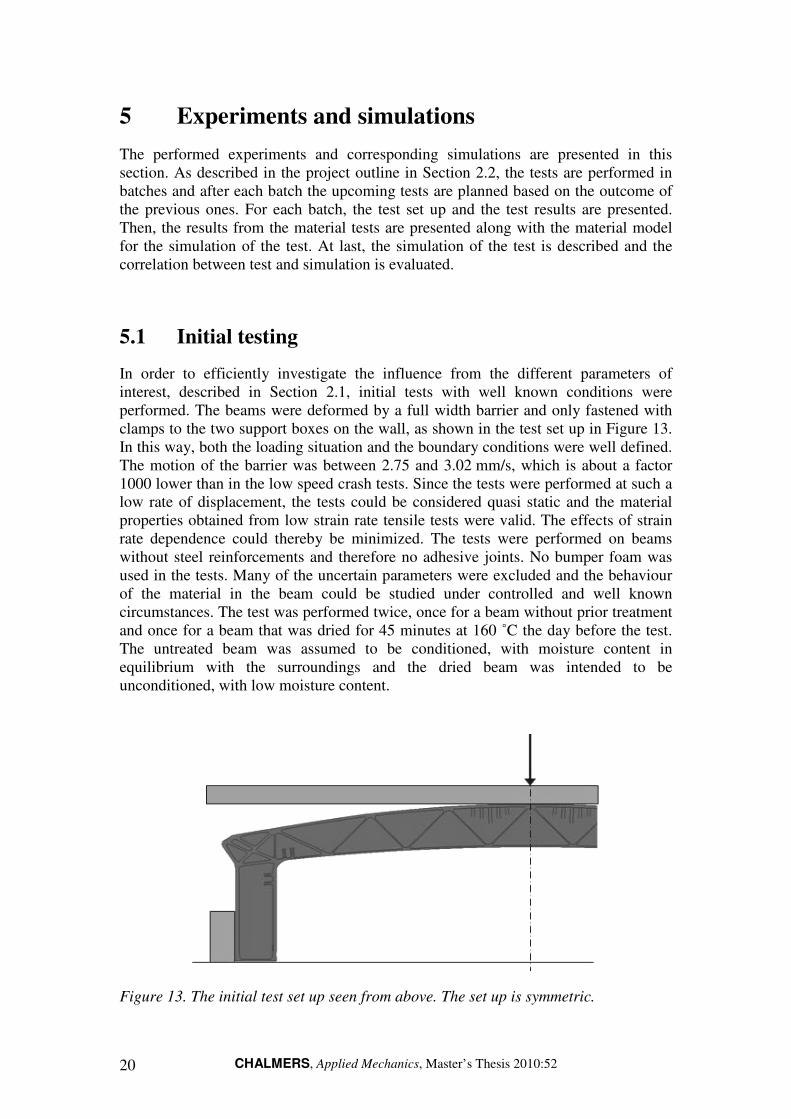
5.1 Initial testing
In order to efficiently investigate the influence from the different parameters of interest, described in Section 2.1, initial tests with well known conditions were performed. The beams were deformed by a full width barrier and only fastened with clamps to the two support boxes on the wall, as shown in the test set up in Figure 13. In this way, both the loading situation and the boundary conditions were well defined. The motion of the barrier was between 2.75 and 3.02 mm/s, which is about a factor 1000 lower than in the low speed crash tests. Since the tests were performed at such a low rate of displacement, the tests could be considered quasi static and the material properties obtained from low strain rate tensile tests were valid. The effects of strain rate dependence could thereby be minimized. The tests were performed on beams without steel reinforcements and therefore no adhesive joints. No bumper foam was used in the tests. Many of the uncertain parameters were excluded and the behaviour of the material in the beam could be studied under controlled and well known circumstances. The test was performed twice, once for a beam without prior treatment and once for a beam that was dried for 45 minutes at 160 ˚C the day before the test. The untreated beam was assumed to be conditioned, with moisture content in equilibrium with the surroundings and the dried beam was intended to be unconditioned, with low moisture content.
Figure 13. The initial test set up seen from above. The set up is symmetric.

CHALMERS, Applied Mechanics, Master’s Thesis 2010:52 21
Figure 14. Beam 10 in the test-set up for the initial tests seen from above.
Contrast markers were placed on different positions on the beams before the tests and the tests were filmed. The markers can then be tracked in the films to see how the beams deform. The beams were originally black, but were painted light gray before the testing to make cracks more visible in the films.
5.1.1 Test results
A pre-test was made on beam number 16, in order to indicate the outcome of the tests. The first fracture appeared under the first junction from the middle under the beam when the barrier displacement is about 26 mm. This corresponded to a force of about 21.8 kN. The beam was loaded further, until complete failure. In the actual test on the conditioned beam, number 10, the first crack appeared at a displacement of 25 mm and a force of 22.5 kN at the same position as in the pre-test. The loading continued until the middle crack lead to fracture and one of the crash boxes broke. The fractured beam can be seen in Figure 15. In Figure 16, the applied force versus displacement curve from the test performed on beam 10 can be seen.
Figure 15. Beam 10 after the test. A crack appeared in the middle and the beam was
loaded further until fracture in the middle and the crash box.

CHALMERS, Applied Mechanics, Master’s Thesis 2010:52 22
Figure 16. The load versus displacement curve from the initial test on beam 10.
In the test on beam number 29, assumed to be unconditioned, the beam broke completely, both in the middle and in the left crash box, at a displacement of 43 mm and a force of 44 kN. It was impossible to detect, from the test or the film, which fracture appeared first. The middle fracture can be seen in Figure 17 and the fractured crash box can be seen in Figure 18.
Figure 17. The middle fracture of beam 29.

CHALMERS, Applied Mechanics, Master’s Thesis 2010:52 23
Figure 18. The fracture in the crash box of beam 29.
5.1.2 Material tests
In order to establish valid material models for each beam for the simulations of the performed experiments, material tests were made at AdManus Materialteknink. Material specimens were taken at different positions of the tested beams; on the front side, on the rear side and in the crash boxes. Pieces were sawed out from the beam and then sawed and rasped to dog-bone shaped specimens. Finally the specimens were polished. Typical specimens, before and after tensile tests, can be seen in Appendix A, in Figure A. 8 and Figure A. 9.
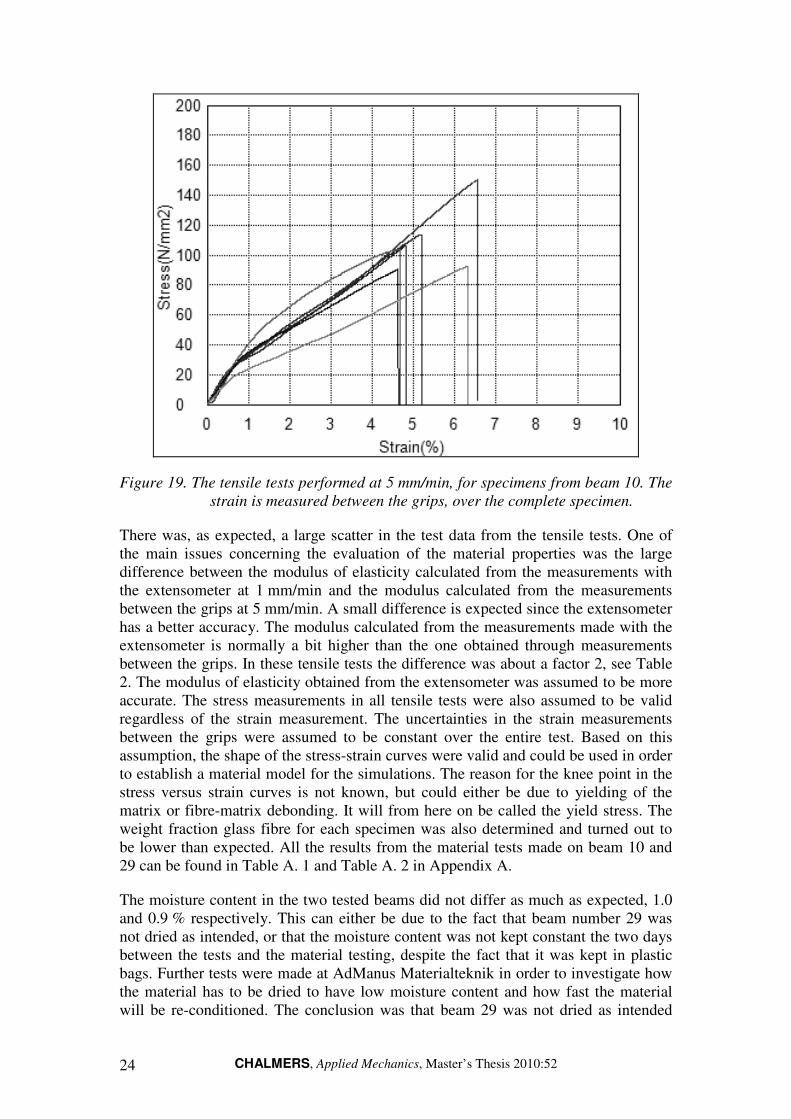
The modulus of elasticity of the material specimens were measured in tensile tests with extensometer at a strain rate of 1 mm/min, corresponding to about 0.0002 s-1. The extensometer measured the strain over a distance of 25 mm. The specimens were strained about 0.1-0.2% and were then unloaded and the modulus was calculated between forces of 100 and 200 N. Next, tensile tests until fracture were performed on the same specimens but at a strain rate of 5 mm/min, about 0.0011 s-1. Due to the risk of damaging the extensometer when fracture occurs, the strain in these tests was measured between the grips holding the specimens. In Figure 19 the stress versus strain curves from the tensile tests until fracture for the specimens from beam 10 are shown. In Appendix A, the stress versus strain curves for the specimens from beam 29 can be seen in Figure A. 3, as well as the testing equipment and the extensometer in Figure A. 10 and Figure A. 11.
CHALMERS, Applied Mechanics, Master’s Thesis 2010:52 24
Figure 19. The tensile tests performed at 5 mm/min, for specimens from beam 10. The
strain is measured between the grips, over the complete specimen.
There was, as expected, a large scatter in the test data from the tensile tests. One of the main issues concerning the evaluation of the material properties was the large difference between the modulus of elasticity calculated from the measurements with the extensometer at 1 mm/min and the modulus calculated from the measurements between the grips at 5 mm/min. A small difference is expected since the extensometer has a better accuracy. The modulus calculated from the measurements made with the extensometer is normally a bit higher than the one obtained through measurements between the grips. In these tensile tests the difference was about a factor 2, see Table 2. The modulus of elasticity obtained from the extensometer was assumed to be more accurate. The stress measurements in all tensile tests were also assumed to be valid regardless of the strain measurement. The uncertainties in the strain measurements between the grips were assumed to be constant over the entire test. Based on this assumption, the shape of the stress-strain curves were valid and could be used in order to establish a material model for the simulations. The reason for the knee point in the stress versus strain curves is not known, but could either be due to yielding of the matrix or fibre-matrix debonding. It will from here on be called the yield stress. The weight fraction glass fibre for each specimen was also determined and turned out to be lower than expected. All the results from the material tests made on beam 10 and 29 can be found in Table A. 1 and Table A. 2 in Appendix A.
The moisture content in the two tested beams did not differ as much as expected, 1.0 and 0.9 % respectively. This can either be due to the fact that beam number 29 was not dried as intended, or that the moisture content was not kept constant the two days between the tests and the material testing, despite the fact that it was kept in plastic bags. Further tests were made at AdManus Materialteknik in order to investigate how the material has to be dried to have low moisture content and how fast the material will be re-conditioned. The conclusion was that beam 29 was not dried as intended

CHALMERS, Applied Mechanics, Master’s Thesis 2010:52 25
and that the moisture content in the beam at the test was about the same as when the material properties were tested. Therefore the material data was assumed to be valid for the simulations of the test.
Table 2. The results from materials tests made on beam 10 and 29. The values are
mean values and the standard deviations are given within
parenthesises.
Beam E1,ext [GPa]
E5 [GPa]
Etan,5 [GPa]
σu,5 [MPa]
εf,5 [%]
GF [wt%]
Moisture [wt%]
10 8.1 (1.7) 4.2 (0.6) 1.7 (0.3) 109 (22) 5.4 (0.9) 32.8 (0.8) 1.0
29 8.5 (1.6) 4.0 (0.7) 1.9 (0.7) 123 (18) 6.0 (0.9) 31.8 (0.8) 0.9
5.1.3 Material models
Before the tests were performed at Saab Automobile AB, some preliminary simulations were made to predict the outcome. A linear elastic material model, MAT_1, was used, with the modulus of elasticity from designing the beam in the previous project, see PA_GF_01 in Table 3. Also a bilinear model, MAT_24 in LS-DYNA, was used based on values from material tests made in March 2010 on beam A2. The bilinear model was used to capture the shape of the stress versus strain curve from the tensile tests. Two sets of parameters for this model, PA_GF_02 and 03, can be seen in Table 3. A brief description of the used material models in LS-DYNA can be found in Appendix C.
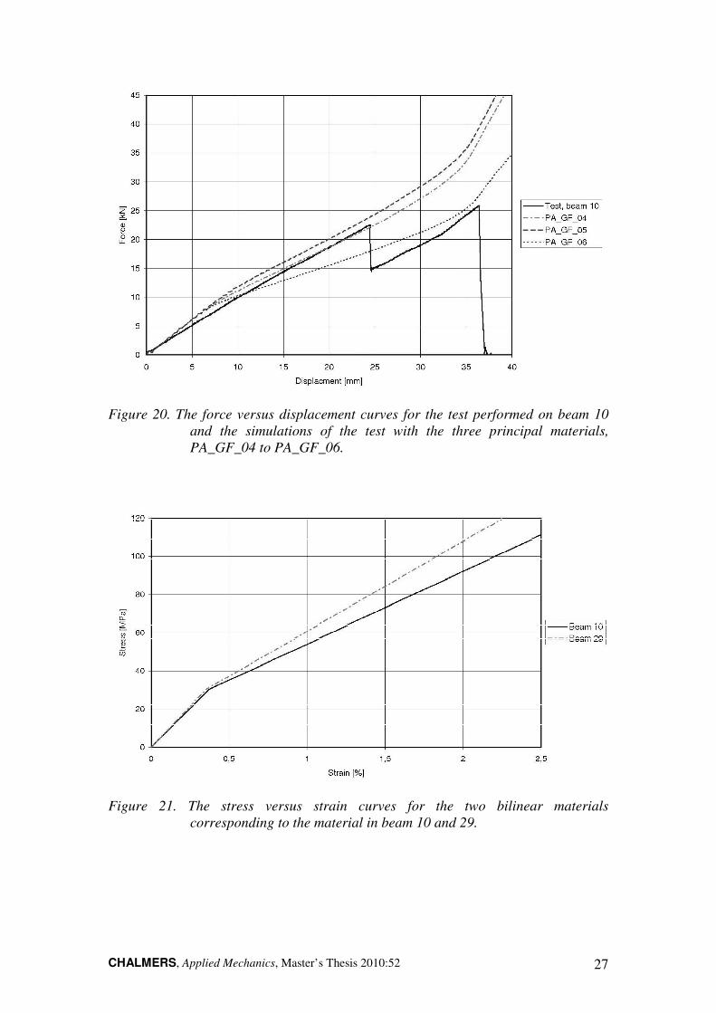
After the material tests described in the previous subsection, the initial tests were simulated with several different materials, all bilinear with isotropic properties. The modulus of elasticity measured with the extensometer was used and the yield stress was taken as the stress where the slope of the curve changes in the tensile tests to fracture, see Figure 19. The ratio between the tangent modulus and the modulus of elasticity from the tensile tests to fracture was found to be rather constant. The mean value of the ratio was 0.407 and 0.473 for beam 10 and 29 respectively, see Table A. 1 and Table A. 2 in Appendix A for more details. Since the tangent modulus was never measured with extensometer, its value was calculated from the modulus of elasticity measured with extensometer and the ratio obtained from the tensile tests without extensometer. This assumption is not generally known and accepted, so to reveal the influence from the yield stress and the tangent modulus, three principal sets of parameters, PA_GF_04 to PA_GF_06 in Table 3, were used in the bilinear material model. The aim was to see if the assumed material gave reasonable results and how much a change in one of the parameters affected the outcome. The densities for these materials were approximated based on the prescribed glass fibre fraction between 37 and 45 wt%. The applied force versus displacement curves from simulations of a beam in the initial test set up made with these principal sets of properties were compared with the corresponding curve from the initial test on beam 10, see Figure 20. It could be concluded that the material model seemed to give a reasonable force versus displacement curve. The dotted curve shows the effect of a lower tangent modulus and the correlation can be seen to be worse than for the other curves. The
CHALMERS, Applied Mechanics, Master’s Thesis 2010:52 26
correlation was better when a tangent modulus of half the modulus of elasticity was used. Based on this, the assumption that the ratio between modulus of elasticity and the tangent modulus can be used for calculating the tangent modulus seems reasonable. The influence from a higher yield stress than the assumed 30 MPa, is not big. It results in a slightly higher level of applied force, the dashed curve. The difference is not so big and therefore the assumption of a yield stress of 30 MPa will not lead to big uncertainties even though there is some variation among the actual yield stresses.
Based on these results, the material in beam 10 and 29 was modelled with the above described assumptions. The last two materials in Table 3 correspond to the material in beam 10 and 29 and the stress versus strain curves for the material model with these parameters can be seen in Figure 21. The density for each of the last two materials was adjusted so that the weight of the beam corresponds to the one given in Table 1.
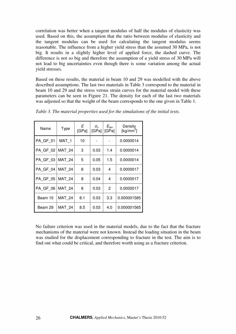
Table 3. The material properties used for the simulations of the initial tests.
No failure criterion was used in the material models, due to the fact that the fracture mechanisms of the material were not known. Instead the loading situation in the beam was studied for the displacement corresponding to fracture in the test. The aim is to find out what could be critical, and therefore worth using as a fracture criterion.
Name Type E
[GPa] σy
[GPa] Etan
[GPa] Density
[kg/mm3]
PA_GF_01 MAT_1 10 - - 0.0000014
PA_GF_02 MAT_24 3 0.03 1.4 0.0000014
PA_GF_03 MAT_24 5 0.05 1.5 0.0000014
PA_GF_04 MAT_24 8 0.03 4 0.0000017
PA_GF_05 MAT_24 8 0.04 4 0.0000017
PA_GF_06 MAT_24 8 0.03 2 0.0000017
Beam 10 MAT_24 8.1 0.03 3.3 0.000001585
Beam 29 MAT_24 8.5 0.03 4.0 0.000001565
CHALMERS, Applied Mechanics, Master’s Thesis 2010:52 27
Figure 20. The force versus displacement curves for the test performed on beam 10
and the simulations of the test with the three principal materials,
PA_GF_04 to PA_GF_06.
Figure 21. The stress versus strain curves for the two bilinear materials
corresponding to the material in beam 10 and 29.

CHALMERS, Applied Mechanics, Master’s Thesis 2010:52 28
5.1.4 Simulations of the initial tests
The initial test set up was simulated with a barrier modelled in a rigid material, MAT_20, deforming the beam with a prescribed motion of 0.3 mm/ms. The prescribed motion is about 100 times larger than the motion in the actual test, but is used in order to reduce the simulation time. This does not influence the simulated results, which is shown in Appendix E. The contact between the barrier and the beam was modelled as automatic surface to surface. In this automatic contact definition a master and a slave part are defined and the contact surfaces are internally generated in LS-DYNA. The wall and the support boxes were also modelled in rigid material. During the tests, the beams were clamped to the supports, but in the simulations the contact between the beam and the supporting boxes were modelled as automatic surface to surface contacts. Most likely, this did not affect the correlation since the more the barrier was displaced, the more the beam was pressed against the supporting boxes, which could be seen from the contact forces in the simulations. It means that the clamps lost their influence, as soon as the deformation started. The materials in the tested beams were modelled as described in the previous subsection. Due to the symmetry, a model of half the beam was used. The simulations were performed in LS-DYNA, version mpp971s.
5.1.5 Correlation between test and simulation for beam 10
Initially, only the first part of the simulation, i.e. the behaviour until the first fracture, was studied. Without a failure criterion, the later part of the test, after the first fracture, has to be treated separately. The first part was the most interesting part for the initial correlation investigations. The force needed to create the prescribed displacement, were compared for the tests and the simulations. The force versus displacement curve from the test performed on beam 10 is plotted together with the curve from the simulation of the test in Figure 22. In the simulation, the force was measured in the contact between the impactor and the beam. The curves can be seen to correlate rather well.
An adequate measure of how loaded the material in the beam is, was assumed to be corresponding to a critical strain where crazing is likely to occur, as described in Section 4.1.1. According to theory, crazing in fibre reinforced polymers occur in the interface between matrix and fibre, and initiate at fibres oriented perpendicular to the stress. If the material is assumed to have more or less random oriented fibres, crazing could start in any direction. Therefore, the maximum principal strain was assumed to be a relevant strain measure. For comparison, also the effective strain was studied as a measure for crazing. In order for crazing to occur, the material must be subjected to hydrostatic tension. To be able to see where crazing was most likely to occur when the beam was deformed, contour plots from the following expression was used, from here on called the modified principal strain,
( )11mod −⋅⋅= εεp
p (5.1)

CHALMERS, Applied Mechanics, Master’s Thesis 2010:52 29
where p is the pressure and ε1 is the maximum principal strain. The first ratio will equal -1 if hydrostatic tension is present and 1 if not. The factor -1 at the end of the expression was added to get the modified strain positive where crazing is likely to appear.
Figure 22. The force versus displacement curves from the initial test of beam 10 and
the corresponding simulation.
In the beginning of the simulations, for small displacements, the highest principal stresses and strains were obtained in the middle under the beam, where the material was subjected to almost uniaxial tensile stress. After a certain displacement in the simulations, around 19 mm, the maximum stresses and strains were instead located in the area where the first fracture appeared, i.e. under the beam near the first junction from the middle, see Figure 15. Fracture is expected, according to the test data, at the time step where the barrier has displaced the beam around 24 mm. At this displacement, the maximum principal stress was 77.6 MPa and the maximal principal strain was 1.76 %, both located in the fracture area. A contour plot of the maximum principal strain modified according to Equation (5.1) for this displacement can be seen in Figure 23. A magnification of the contour plot for the location where the first fracture occurred can be seen in Figure 24. It can be concluded that the location where crazing was most likely to occur according to the simulation, coincided with the location where the first fracture occurred in the test and the strain was 1.76 %. If instead the effective strain was used in the expression, the maximum value was 1.62 %, still at the same location. The overall distribution in the contour plot was not changed radically when the effective strain was used and the fracture region was still the most critical region. The maximum effective stress, according to von Mises, at this displacement was 128.8 MPa and was located on the inside of the corner of the beam. At the fracture location the effective stress was 75.5 MPa.

CHALMERS, Applied Mechanics, Master’s Thesis 2010:52 30
The maximum principal stresses, as well as the effective stress, at the fracture location were lower than the ultimate tensile stresses obtained in the material tests. The ultimate tensile stress might have been a bit lower in the junctions compared to the walls of the beam, where the material data were collected. It can also be due to pores in the junction, which would lead to that the actual stresses in the material were higher than the ones in the simulations. The fibre orientation does also most likely differ between the junctions and the walls.
Figure 23. The contour plot of the modified principal strain, according to
Equation (5.1), in the beam at a barrier displacement of 24 mm,
corresponding to the first fracture in the test.
Figure 24. A magnification of the fracture location from the contour plot in Figure
23. The arrow indicates the location of the maximum value.

CHALMERS, Applied Mechanics, Master’s Thesis 2010:52 31
In order to investigate the behaviour of the beam after the first fracture, simulations were made on a beam with a created crack. The elements were removed in the area where the first crack appeared. It was hard to determine from the film exactly how large the crack was, so several simulations with different amount of damage were investigated. The simulation with a crack almost through the entire beam gave the best correlation between the force versus displacement curves, see Figure 25. The simulation on the damaged beam was made on a complete beam model since it was no more symmetric.
In Figure 25, one can notice that the difference in force between the beam without and with damage is rather small for large displacements, i.e. larger than 35 mm. This was most likely an effect of the load situation, since for large displacements the beam was straightened out and most of the load was transferred to the crash boxes. This occurred a bit earlier in the simulations than in the test due to geometrical differences between the FE-model and the physical beam. When the film from the test and the simulations were compared, the main characteristics of behaviour of the beam after the first crack can be seen.
Figure 25. Force versus displacement from the test of beam 10 and corresponding
curves from the simulations made with a whole and a damaged beam.
The middle section of the beam was not in contact with the barrier anymore, neither in the test nor the simulation. The stress distribution in the beam was changed due to the induced crack. There were stress and strain concentrations at the crack tip, as expected. Except for the region around the crack tip, the crash boxes were subjected to large principal stresses and strains. When studying the modified principal strain, the maximum is obtained at the crack tip. If this area were excluded from the investigation, other parts subjected to rather high strains could be determined. Values around 1.9 % were obtained on the outside of the crash box and values above 2 % were obtained in the middle wall in the crash box. It seemed quite reasonable, compared to the actual second fracture, see Figure 15. A contour plot for the modified
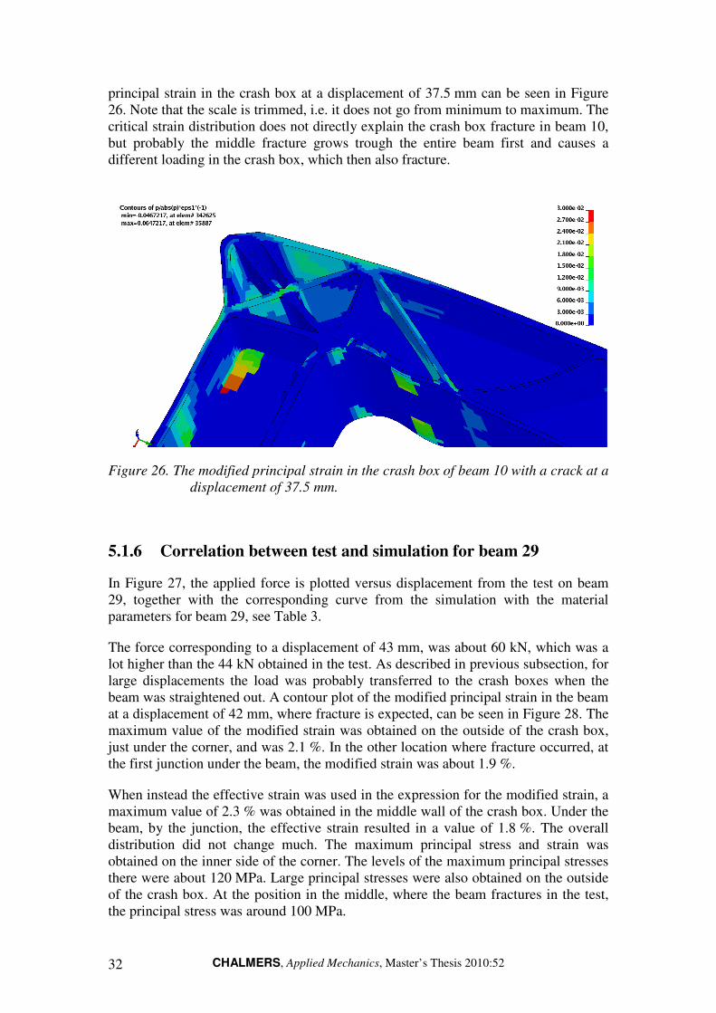
CHALMERS, Applied Mechanics, Master’s Thesis 2010:52 32
principal strain in the crash box at a displacement of 37.5 mm can be seen in Figure 26. Note that the scale is trimmed, i.e. it does not go from minimum to maximum. The critical strain distribution does not directly explain the crash box fracture in beam 10, but probably the middle fracture grows trough the entire beam first and causes a different loading in the crash box, which then also fracture.
Figure 26. The modified principal strain in the crash box of beam 10 with a crack at a
displacement of 37.5 mm.
5.1.6 Correlation between test and simulation for beam 29
In Figure 27, the applied force is plotted versus displacement from the test on beam 29, together with the corresponding curve from the simulation with the material parameters for beam 29, see Table 3.
The force corresponding to a displacement of 43 mm, was about 60 kN, which was a lot higher than the 44 kN obtained in the test. As described in previous subsection, for large displacements the load was probably transferred to the crash boxes when the beam was straightened out. A contour plot of the modified principal strain in the beam at a displacement of 42 mm, where fracture is expected, can be seen in Figure 28. The maximum value of the modified strain was obtained on the outside of the crash box, just under the corner, and was 2.1 %. In the other location where fracture occurred, at the first junction under the beam, the modified strain was about 1.9 %.
When instead the effective strain was used in the expression for the modified strain, a maximum value of 2.3 % was obtained in the middle wall of the crash box. Under the beam, by the junction, the effective strain resulted in a value of 1.8 %. The overall distribution did not change much. The maximum principal stress and strain was obtained on the inner side of the corner. The levels of the maximum principal stresses there were about 120 MPa. Large principal stresses were also obtained on the outside of the crash box. At the position in the middle, where the beam fractures in the test, the principal stress was around 100 MPa.

CHALMERS, Applied Mechanics, Master’s Thesis 2010:52 33
Figure 27. The force versus displacement curves from the test and the corresponding
simulation for beam 29.
Figure 28. The modified principal strain distribution in beam 29 at a displacement of
42 mm.
Altogether, the correlation of the results from the initial tests and the corresponding simulations were satisfactory. The correlation for the force versus displacement curves, turned out to be satisfactory when an isotropic, bilinear material model was used. The conclusion was that if the properties were obtained from the actual beam material, the used material model did not cause large uncertainties. Which fracture criterion to use in order to predict the fracture in a proper way was not clarified. However, the critical strain was assumed to be the most reliable measure so far. The obtained values for the modified principal strain, according to Equation (5.1), where the fractures were expected, were in the range 1.76 and 1.9 %. The maximum of the modified principal strain was not always located where the fracture occurred.
CHALMERS, Applied Mechanics, Master’s Thesis 2010:52 34
5.2 Testing of strain rate dependence
In order to be able to design load bearing components in short glass fibre reinforced polyamide, the strain rate dependence must be determined. Equipment for high strain rate tensile testing in order to obtain material properties at high strain rates was not available within this project. In order to reveal the dynamic effects in the material, tests on beams were performed. The aim was to hold all test conditions, except the loading rate, constant in two tests. Beam 26 and 27 were chosen for the tests. Both were manufactured late in the production series and with the same process parameters, which should result in beams with similar properties. The beams were assumed to have about the same fraction glass fibre.
The first of the two tests was the same as the ones performed in the initial testing, except that a circular impactor was used instead of the barrier. This change was made since the circular impactor was supposed to give a better defined load situation. At the same time, one more load situation is available to verify the simulation of the quasi static behaviour of the material. The test set up can be seen in Figure 29.
In the dynamic version of the test, the beam was fastened to a cart, which was driven with a velocity of 2.5 m/s into the circular impactor, see Figure 29. The weight of the cart was 1000 kg. The cart was driven until the cart was 500 mm away from the wall. At a distance of 800 mm from the wall, the velocity was measured over a distance of 60 mm. Additionally, the position of the cart was measured with a laser measurement equipment and an accelerometer was placed on the cart. Behind the wall, six force sensors were placed. The weight of the wall was estimated to 560 kg and the impactor has a weight of 68 kg.
Figure 29. The set ups for the tests aiming to reveal the strain rate effects. The quasi
static test (left) is as the initial test but with a circular impactor. In the
impact test (right), the beam is fastened on a moving cart and the
circular impactor is fastened on the wall.
5.2.1 Test results
The quasi static test with the circular impactor, was performed on beam 27 and the test equipment can be seen in Figure 30. The beam fractured at the same position as in

CHALMERS, Applied Mechanics, Master’s Thesis 2010:52 35
the previous tests, i.e. in the first junction from the middle under the beam. The displacement of the impactor was about 25 mm and the corresponding force about 17.5 kN.
Figure 30. The test set up for the quasi static test with the circular impactor.
In Figure 31, beam 26 can be seen placed in the cart for the dynamic impact test. In the test, the beam broke entirely about 10 ms after the first contact between the beam and the impactor. The velocity of the cart was measured to 9.11 km/h, i.e. 2.53 m/s, at a distance of 800 mm from the wall. The accelerometer measurement turned out to be less significant for the determination of the velocity of the cart, due to vibrations and other disturbances. The laser measurement equipment did not work properly at the test occasion.
The force measured behind the wall, in which the cart drove, was just above 20 kN at the time for the fracture. The fractured beam can be seen in Figure 32. The responses from the quasi static and the impact test can be compared in Figure 33. Assuming the same material properties in both tested beams, a stiffening effect can be seen in the beam subjected to the higher deformation rate. This behaviour is reasonable and expected according to literature, see Section 4.3.
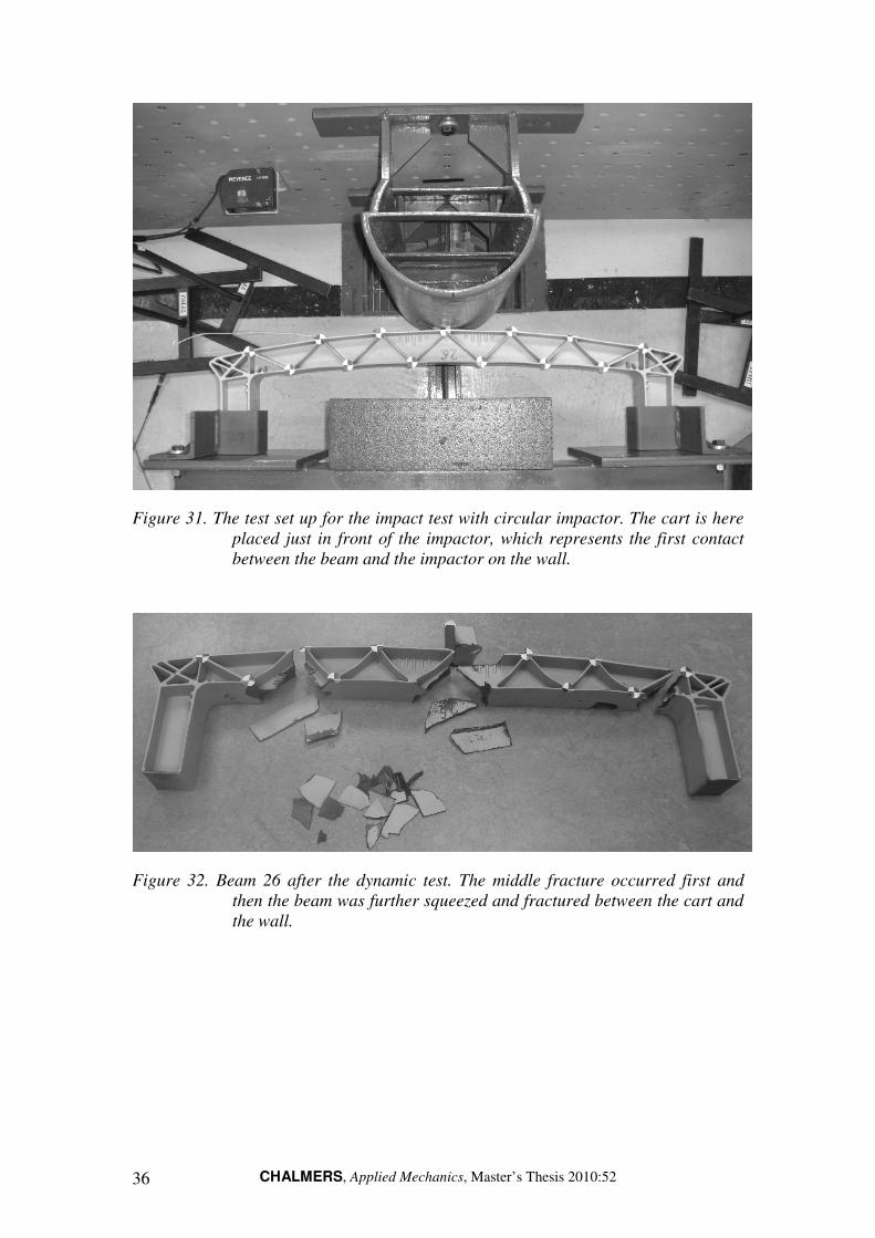
CHALMERS, Applied Mechanics, Master’s Thesis 2010:52 36
Figure 31. The test set up for the impact test with circular impactor. The cart is here
placed just in front of the impactor, which represents the first contact
between the beam and the impactor on the wall.
Figure 32. Beam 26 after the dynamic test. The middle fracture occurred first and
then the beam was further squeezed and fractured between the cart and
the wall.

CHALMERS, Applied Mechanics, Master’s Thesis 2010:52 37
Figure 33. The force versus displacement measured in the quasi static and the
dynamic impact test.
5.2.2 Material tests and models
The material in the tested beams was investigated in tensile tests at AdManus Materialteknik, following the same procedure as after the initial tests, described in Section 5.1.2. The stress versus strain curves from the 5 mm/min tensile tests to fracture can be seen in Figure A. 4 and Figure A. 5, in Appendix A. Large differences between strain measurements with the extensometer and between the grips were present in these tests, as in the ones for beam 10 and 29. The material in beam 26 and 27 turned out to be less stiff compared to beam 10 and 29. The lower modulus of elasticity was probably caused by the lower glass fibre fraction in these beams, namely 23.3 wt% and 21.9 wt% for beam 26 and 27 respectively. The main results from the tests made on beam 26 and 27 can be seen in Table 4 and all the results can be seen in Appendix A, Table A. 3 and Table A. 4. The stress versus strain curves from the tensile tests performed to fracture can be seen in Figure A. 4 and Figure A. 5.
Table 4. The results from materials tests made on beam 26 and 27. The values are
mean values and the standard deviations are given within
parenthesises.
Beam E1,ext [GPa]
E5 [GPa]
Etan,5 [GPa]
σu,5 [MPa]
εf,5 [%]
GF [wt%]
26 5.5 (1.1) 3.7 (0.5) 1.6 (0.4) 97 (14) 5.0 (0.9) 23.3 (0.9)
27 6.1 (1.1) 4.2 (0.6) 1.9 (0.5) 103 (13) 4.3 (0.4) 21.9 (0.4)

CHALMERS, Applied Mechanics, Master’s Thesis 2010:52 38
From the properties obtained, two sets of parameters for the bilinear material model were established. These parameters can be seen in Table 5. Also, for these parameters the ratio between the tangent modulus and the modulus of elasticity was used together with the modulus of elasticity obtained from the measurements with the extensometer. A slightly higher yield stress could be seen in the curves from these tests and a yield stress of 35 MPa was used for the simulations. The densities were set to give the known mass of the beams.
Table 5. The material properties used in the bilinear model for the simulations of
beam 26 and 27.
5.2.3 Simulation and correlation of the quasi static test
The simulation of the quasi static test with the circular impactor was performed as the previous simulations, but with a circular impactor in rigid material instead of the barrier. The motion of the impactor was prescribed to be 0.3 mm/ms and the wall supports were modelled as rigid. The contact between the beam and the impactor, as well as the contact between the beam and the wall, was modelled as automatic surface to surface contacts. Only half the test set up was modelled due to symmetry. The simulation was performed in LS-DYNA, version mpp971s.
In Figure 34 the applied force versus the displacement curves from the test on beam 27 and the corresponding simulation are plotted. As in the evaluation of the initial tests, the modified principal strain introduced in Equation (5.1) was used. The beam was studied at a displacement of 24 mm. The contour plot of the modified principal strain can be seen in Figure 35. The maximum value of the modified principal strain was obtained in the middle under the beam and was 2.2 %. At the failure location, a modified strain of 1.9 % was obtained. If the effective strain was used in Equation (5.1), values of 2.0 % in the middle under the beam and 1.8 % in the fracture region were obtained. A highest principal stress of 81.2 MPa was obtained in the middle under the beam. At this displacement, the maximal principal stress was 74.0 MPa under the first junction. The maximum shear stress at this time step was obtained on the inside of the corner and was 56.2 MPa.
Name Type E
[GPa] σy
[GPa] Etan
[GPa] Density
[kg/mm3]
Beam 26 MAT_24 5.5 0.035 2.3 0.00000147
Beam 27 MAT_24 6.1 0.035 2.7 0.000001455

CHALMERS, Applied Mechanics, Master’s Thesis 2010:52 39
Figure 34. The force versus displacement for the quasi static test and the
corresponding simulation for beam 27.
Figure 35. A contour plot of the modified principal strain at a displacement of 24 mm
in the simulation of the quasi static test.
5.2.4 Simulation and correlation of the dynamic test
For the dynamic test the entire test rig was simulated in order to capture the fact that the wall was not completely rigid, i.e. the wall moved when the cart hit it. Instead of a

CHALMERS, Applied Mechanics, Master’s Thesis 2010:52 40
prescribed motion, the cart was given the initial velocity and the mass of the cart. Behind the model of the wall, which was given the mass of the wall in the test set up, a beam element was used to connect the wall to a fixed piece of wall positioned a bit further back. The axial force in the beam element could then be compared to the force measured in the six sensors behind the wall. The material in the beam element was chosen in order to show critical damping. Only half the test set up was modelled in the simulations due to symmetry.
In Figure 36, the force measured behind the wall is plotted versus the displacement of the middle of the beam, both for the test and the simulation. The fluctuations in the curve from the simulation were due to the fact that the beam started to oscillate as it hit the impactor. The same tendency can be seen in the curve from the test, although the system is more damped. No damping was included in the simulation.
Since the measurements from the accelerometer can not be used, the velocity of the cart is not completely known throughout the crash. However, the large mass of the cart compared to the relatively weak beam made it reasonable to believe that the velocity of the cart was more or less constant from contact to fracture. The time and velocity was used to calculate the displacement of the beam, in order to make the different tests comparable.
Figure 36. The force measured behind the wall in the dynamic test and the
corresponding force from the simulation, as functions of displacement.
The displacement of the beam is zero when the beam first gets in
contact with the impactor. The displacement in the test is calculated
from assumed velocity, in order to make the curves comparable.
The loading situation in the beam was studied 10 ms after the first contact, since then fracture was expected. The distribution of the modified principal strain was similar to the one obtained in the simulation of the quasi static test, see Figure 41. The

CHALMERS, Applied Mechanics, Master’s Thesis 2010:52 41
maximum value was obtained in the middle under the beam and was 2.3 %. In the region where the first fracture occurs, the value was around 1.9 %. When using the effective strain, the values instead were 2.1 % and 1.8 % respectively. The largest maximum principal stress was located under the beam and was 75.9 MPa. In the fracture region, it was 66.8 MPa.
When taking into consideration that the material in the dynamic tested beam turned out to be less stiff than the material in the quasi static tested one, the stiffening effect seen in Figure 33 can be assumed to be even larger. From just comparing the measured forces prior to the fractures in each test, the stiffening effect can be estimated to about 20 %. If a higher modulus of elasticity is assumed to cause a higher force, proportional to the ratio of moduluses, the stiffening effect can be estimated to be around 30 % from comparing two equivalent stiff beams. Due to the fact that only one dynamic test was performed, the measurements were rather uncertain and oscillations were present, these figures are intended to be a estimation of the magnitude of the effect, rather than a verified result for the beam material.
Figure 37. The contour plot of the modified maximum principal strain from the
simulations of the dynamic tested beam, number 26, at the time 10 ms.
5.3 Testing with asymmetric loading
All the tested beams so far were tested with a symmetric loading and the first fracture in all quasi static tests were located at the same position in the beams. The quality of the material in the junctions compared to other parts of the beam was not known and the main fracture mechanisms were not determined. By adding an asymmetric load distribution probably another fracture location will take place. Therefore, an asymmetric test was performed. The test was performed quasi statically, since it was

CHALMERS, Applied Mechanics, Master’s Thesis 2010:52 42
then easier to control the test situation and obtain measurements without much disturbances, compared to a dynamically performed test.
5.3.1 Test results
Beam 18 was tested in an asymmetric test set up, which can be seen in Figure 38. The first fracture in the beam occurred at the junction on the rear side, opposite to the point where the beam was loaded, see Figure 39, at a displacement of 22.7 mm and a force of 19.6 kN. The beam was then just loaded a bit further before the test was interrupted.
Figure 38. The test set up where beam 18 is asymmetrically loaded.
Figure 39. The tested beam just after the fracture, which occurred on the rear side,
opposite from the loading point. The picture is taken from the film.
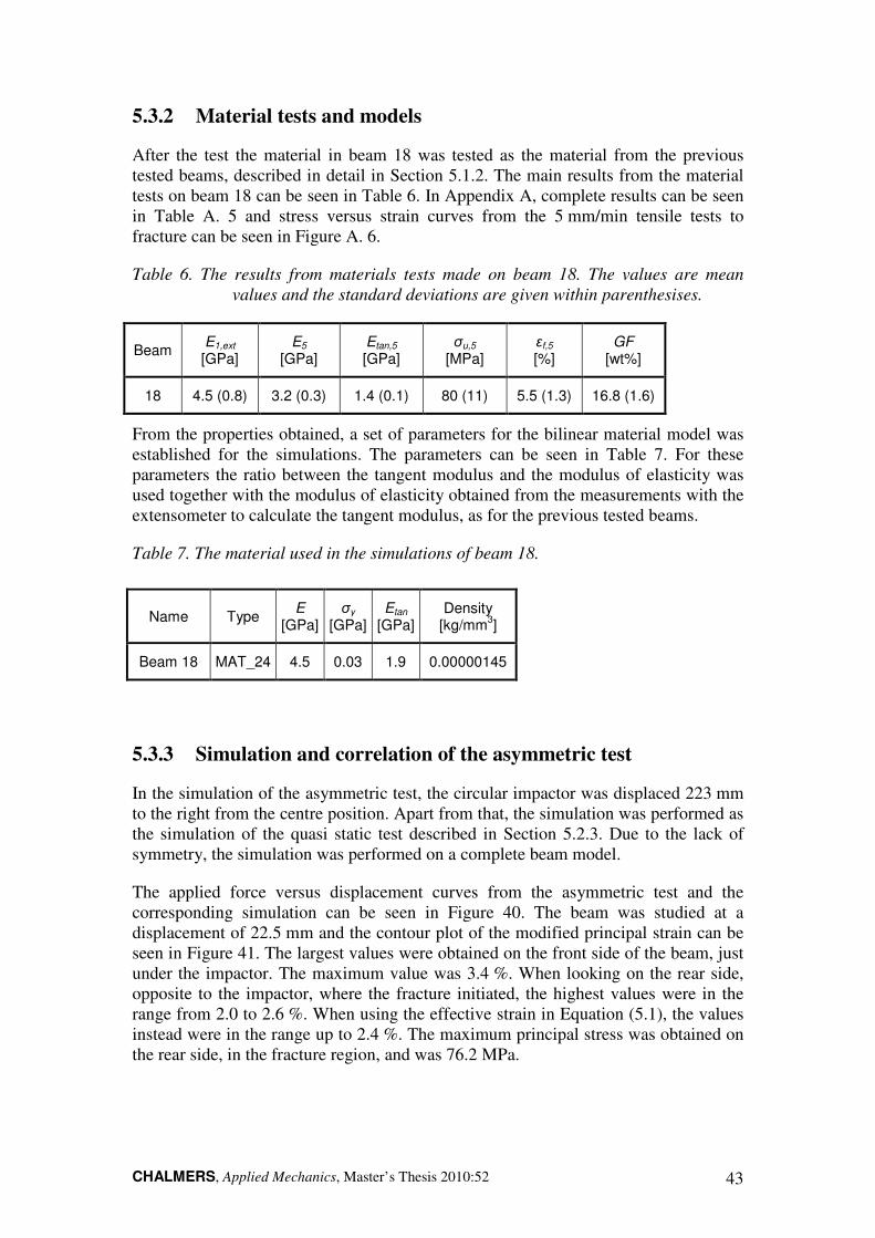
CHALMERS, Applied Mechanics, Master’s Thesis 2010:52 43
5.3.2 Material tests and models
After the test the material in beam 18 was tested as the material from the previous tested beams, described in detail in Section 5.1.2. The main results from the material tests on beam 18 can be seen in Table 6. In Appendix A, complete results can be seen in Table A. 5 and stress versus strain curves from the 5 mm/min tensile tests to fracture can be seen in Figure A. 6.
Table 6. The results from materials tests made on beam 18. The values are mean
values and the standard deviations are given within parenthesises.
Beam E1,ext [GPa]
E5 [GPa]
Etan,5 [GPa]
σu,5 [MPa]
εf,5 [%]
GF [wt%]
18 4.5 (0.8) 3.2 (0.3) 1.4 (0.1) 80 (11) 5.5 (1.3) 16.8 (1.6)
From the properties obtained, a set of parameters for the bilinear material model was established for the simulations. The parameters can be seen in Table 7. For these parameters the ratio between the tangent modulus and the modulus of elasticity was used together with the modulus of elasticity obtained from the measurements with the extensometer to calculate the tangent modulus, as for the previous tested beams.
Table 7. The material used in the simulations of beam 18.
5.3.3 Simulation and correlation of the asymmetric test
In the simulation of the asymmetric test, the circular impactor was displaced 223 mm to the right from the centre position. Apart from that, the simulation was performed as the simulation of the quasi static test described in Section 5.2.3. Due to the lack of symmetry, the simulation was performed on a complete beam model.
The applied force versus displacement curves from the asymmetric test and the corresponding simulation can be seen in Figure 40. The beam was studied at a displacement of 22.5 mm and the contour plot of the modified principal strain can be seen in Figure 41. The largest values were obtained on the front side of the beam, just under the impactor. The maximum value was 3.4 %. When looking on the rear side, opposite to the impactor, where the fracture initiated, the highest values were in the range from 2.0 to 2.6 %. When using the effective strain in Equation (5.1), the values instead were in the range up to 2.4 %. The maximum principal stress was obtained on the rear side, in the fracture region, and was 76.2 MPa.
Name Type E
[GPa] σy
[GPa] Etan
[GPa] Density
[kg/mm3]
Beam 18 MAT_24 4.5 0.03 1.9 0.00000145

CHALMERS, Applied Mechanics, Master’s Thesis 2010:52 44
Figure 40. The applied force versus displacement for beam 18 from the test and the
simulation.
Figure 41. A contour plot of the modified principal strain in the simulation of the
asymmetric test on beam 18 at a displacement of 22.5 mm.
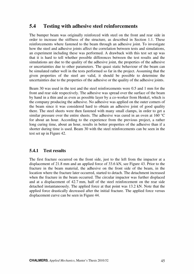
CHALMERS, Applied Mechanics, Master’s Thesis 2010:52 45
5.4 Testing with adhesive steel reinforcements
The bumper beam was originally reinforced with steel on the front and rear side in order to increase the stiffness of the structure, as described in Section 1.1. These reinforcements where fastened to the beam through an adhesive joint. To investigate how the steel and adhesive joints affect the correlation between tests and simulations, an experiment including these was performed. A drawback with this test set up was that it is hard to tell whether possible differences between the test results and the simulations are due to the quality of the adhesive joint, the properties of the adhesive or uncertainties due to other parameters. The quasi static behaviour of the beam can be simulated rather well in the tests performed so far in the project. Assuming that the given properties of the steel are valid, it should be possible to determine the uncertainties due to the properties of the adhesive or the quality of the adhesive joints.
Beam 30 was used in the test and the steel reinforcements were 0.5 and 1 mm for the front and rear side respectively. The adhesive was spread over the surface of the beam by hand in a thin and as even as possible layer by a co-worker from Henkel, which is the company producing the adhesive. No adhesive was applied on the outer corners of the beam since it was considered hard to obtain an adhesive joint of good quality there. The steel sheets were then fastened with many small clamps, in order to get a similar pressure over the entire sheets. The adhesive was cured in an oven at 160 °C for about an hour. According to the experience from the previous project, a rather long curing time, about an hour, results in better properties of the adhesive than if a shorter during time is used. Beam 30 with the steel reinforcements can be seen in the test set up in Figure 42.
5.4.1 Test results
The first fracture occurred on the front side, just to the left from the impactor at a displacement of 21.8 mm and an applied force of 33.6 kN, see Figure 43. Prior to the fracture in the beam material, the adhesive on the front side of the beam, in the location where the fracture later occurred, started to detach. The detachment increased when the fracture in the beam occurred. The circular impactor was further displaced and at a displacement of 42.7 mm, half of the steel reinforcement on the rear side detached instantaneously. The applied force at that point was 13.2 kN. Note that the applied force drastically decreased after the initial fracture. The applied force versus displacement curve can be seen in Figure 44.

CHALMERS, Applied Mechanics, Master’s Thesis 2010:52 46
Figure 42. The test set up for beam 30 with the adhesive steel reinforcements.
Figure 43. The fracture in the steel reinforced beam, the picture is taken from the film
of the test.

CHALMERS, Applied Mechanics, Master’s Thesis 2010:52 47
5.4.2 Material tests and models
After the test, the material in beam 30 was tested in the same ways as the material from the previous tested beams, as described in detail in Section 5.1.2. The main results from the material tests can be seen in Table 8. In Appendix A, more results can be seen in Table A. 6 as well as the stress versus strain curves from the 5 mm/min tensile tests to fracture in Figure A. 7.
Table 8. The results from materials tests made on beam 30. The values are mean
values and the standard deviations are given within parenthesises.
Beam E1,ext [GPa]
E5 [GPa]
Etan,5 [GPa]
σu,5 [MPa]
εf,5 [%]
GF [wt%]
30 8.8 (1.3) 4.9 (1.5) 2.2 (0.2) 125 (21) 5.0 (0.8) 30.5 (0.5)
From the properties obtained, a set of parameters for the bilinear material model was established. The parameters can be seen in Table 9. The same assumption regarding the calculation of the tangent modulus, as for the previous tested beams, was made.
Table 9. The material used in the simulations of beam 30.
The actual material properties of neither the steel nor the adhesive were tested within this project. The HyTens 1200 stainless steel material has a high yield stress and a relatively high ductility. The steel was modelled with a material of model MAT_24, piecewise linear plasticity, with load curves including some strain rate hardening.
The adhesive Terokal 50895 is a structural adhesive with a base of epoxy resin, with high peel and impact peel resistance. In these simulations, the adhesive layer was modelled with a layer of cohesive elements with the cohesive material model MAT_185. The mechanical behaviour of adhesives is often described through a stress-deformation relation. A typical relation for this material model and a further description can be found in Appendix C.
5.4.3 Simulation and correlation of test
The test with adhesive steel reinforcements was simulated as the previous quasi static test with circular impactor. The impactor and the wall and supports were modelled in rigid material. The impactor deformed the beam with a deformation rate of 0.3 mm/ms. The contacts between the impactor and the steel reinforcement in front of
5 Terokal 5089 has replaced Terokal 5087.
Name Type E
[GPa] σy
[GPa] Etan
[GPa] Density
[kg/mm3]
Beam 30 MAT_24 8.8 0.03 4.4 0.000001565
CHALMERS, Applied Mechanics, Master’s Thesis 2010:52 48
the beam as well as the supporting wall and the beam were modelled as automatic surface to surface. The steel sheets were modelled with shell element of corresponding thicknesses. Between the solid elements in the beam and the shell elements in the steel sheets a layer of solid, cohesive elements were used in order to model the adhesive. For these elements, an interior contact was used, in order to avoid elements with negative volumes when subjected to large deformations. The interior contact prevents further deformation when the element is deformed to a certain fraction of the original thickness. Additional, an eroding single surface contact was used, on a set including the beam, the steel and the adhesive, in order to handle the situation where the steel touches the beam after the cohesive elements have failed due to too large stresses.
When the beam was tested with the adhesive steel reinforcements, several uncertainties could not be avoided. All the prior uncertainties, such as the material quality, the assumed isotropy of the material and the bilinear material model, were of course still present. Additional, the properties of the adhesive were not validated and the quality of the adhesive joint could not be assured. In the simulations of the test, the uncertainties due to modelling of the adhesive were added. As for the previous tests, the contact force as a function of displacement was studied. However in addition, it was also of great importance to capture the behaviour of the adhesive, in terms of where and when it detached.
First, a simulation of the test was made where the properties of the adhesive defined in the previous project were used, see simulation 1 in Figure 44. The steel reinforcement in the simulation did only detach in the ends of the on the rear side of the beam and the first detachment seen in the test on the front side could not be seen at all in the simulation. Based on this, several simulations were made with different parameters for the adhesive in order to see how the real behaviour of the adhesive in the test could be captured. However, the responses in the simulations were too stiff and the force versus displacement curves did not correlate well. The adhesive in the simulations did detach much later than in the test and the detachment did not initiate in the same region as in the test. Despite varying the parameters in the cohesive model, the accurate behaviour could not be simulated.
The adhesive seemed most loaded on the outer sides on the rear side of the beam, and therefore detached there before it detached on the front side in all simulations. Due to this, another approach was chosen. Since the adhesive on the front side left from the impactor detached early in the test, in an area where the loading probably was not that high, the assumption was made that the adhesive there might have been of poor quality. A simulation was made, where the adhesive simply was removed from that area. It resulted in a less stiff response of the beam and the force versus displacement curve did correlate better with the curve from the test. The sudden decrease in force seen in the simulation and at almost the same time as in the test, was however due to two different reasons. The decrease in the test was mainly due to the fact that the beam fractured on the front side and probably just partly due to that the detachment of the adhesive grew a bit. Still no fracture criterion was used in the material in the simulation, so the entire decrease in force in the curve from the simulation was due to further detachment of the adhesive on the front side of the beam. At the point in the simulation where the beam was supposed to fracture according to the test, the material in the beam was studied. The material in the beam was not highly loaded. The levels
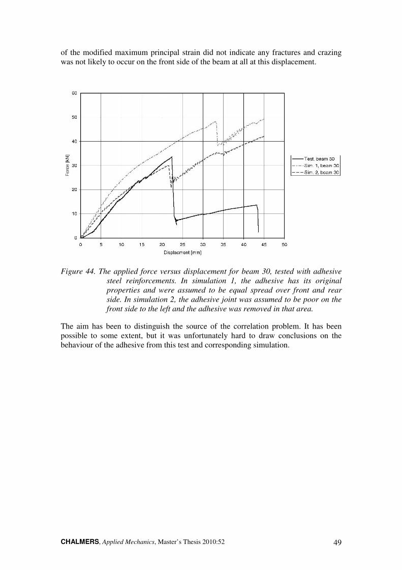
CHALMERS, Applied Mechanics, Master’s Thesis 2010:52 49
of the modified maximum principal strain did not indicate any fractures and crazing was not likely to occur on the front side of the beam at all at this displacement.
Figure 44. The applied force versus displacement for beam 30, tested with adhesive
steel reinforcements. In simulation 1, the adhesive has its original
properties and were assumed to be equal spread over front and rear
side. In simulation 2, the adhesive joint was assumed to be poor on the
front side to the left and the adhesive was removed in that area.
The aim has been to distinguish the source of the correlation problem. It has been possible to some extent, but it was unfortunately hard to draw conclusions on the behaviour of the adhesive from this test and corresponding simulation.
CHALMERS, Applied Mechanics, Master’s Thesis 2010:52 50
6 Updated simulations of previous crash tests
The material properties in the physical beam appeared to differ a lot from what was expected when designing the beam. It is of interest to investigate to what extent the correlation problems were caused by that. The aim with this section is not a new, complete analysis of the crash tests made in the previous project, but rather to estimate how the correlation problems could be reduced with a more accurate material model. This is done by performing some updated simulations. The influence from boundary conditions will also be investigated by including a larger part of the car in a simulation for comparison.
6.1 Crash test simulations with updated material model
A linear elastic material model, with the properties from designing the beam, was used in the simulations of the crash tests in the previous project. The modulus of elasticity was 10 GPa in those simulations. Some tensile tests, performed on the beam material prior to this project, indicated a modulus of elasticity around 6.7 GPa. To establish an updated material model with properties more likely to be valid, the material model was changed to a bilinear material model. The properties were based on the mean of the properties of beam 26, 27 and 29. The modulus of elasticity was 6.7 GPa, the yield stress 35 MPa and the tangent modulus 3.0 GPa. The density was left unchanged, since the mass of the beam was not known. No failure criterion was used in the material model.
According to the test standards for CMVSS215, three tests are performed in a series. Two tests with an offset pendulum are performed on each side of the beam, one in a high (20”) and one in a low (16”) position. The last test is one with a full width barrier. In all tests the velocity is 8 km/h. In the simulations of the two pendulum tests, the entire beam is modelled in the simulation, due to the lack of symmetry. In the barrier test, the symmetry is used and only a model of half the beam is used, see Figure 45. In all three simulations, the beam is fastened with four bolts through each crash box, which are simulated to be fixed in space in the ends. The simulations were performed in LS-DYNA, version ls971s, since it can handle the cohesive elements used for the adhesive joints.
The force as a function of deformation from the crash tests and the simulations for the three different tests are shown in Figure 46 to Figure 48. Also, the results from the simulations in the previous project are included for comparison.

CHALMERS, Applied Mechanics, Master’s Thesis 2010:52 51
Figure 45. The model used for the barrier test seen in ANSA. Boundary constraints
are indicated with blue arrows.
Figure 46. The force versus displacement curve from the crash test with the low
pendulum, fpt16_16, together with the corresponding curves from the
old and updated simulations.

CHALMERS, Applied Mechanics, Master’s Thesis 2010:52 52
Figure 47. The force versus displacement curve from the crash test with the high
pendulum, fpt16_20, together with the corresponding curves from the
old and updated simulations.
Figure 48. The force versus displacement curve from the crash test with the barrier,
fls15, together with the corresponding curves from the old and updated
simulations.
When comparing the updated simulations with the old ones, from the previous project, the slope of the force versus displacement curves is lower. For the crash tests with the low pendulum and the barrier, the correlation between the new simulations and the test data is better than between the test data and the old simulations. For the high pendulum test, the shapes of the force versus displacement curves do not have

CHALMERS, Applied Mechanics, Master’s Thesis 2010:52 53
the same shape as the curve from the test data. This might be an effect of the bumper beam foam used. The foam is not vertical symmetric and when the pendulum is placed in the high position the beam might not be loaded as intended.
6.2 Simulation including a larger part of the car
In the simulations of the crash tests, the beam model was fastened with modelled bolts through the crash boxes. The ends of the bolts were modelled as fixed in space, as described in the previous subsection. In order to see how these simplified boundary conditions, affected the results, the barrier test was simulated once more including a larger part of the car, see Figure 49. The ends of the side beams were simulated to be fixed in space, indicated with arrows in the figure. Even for this simulation, the new bilinear material model was used. In the simulation the barrier hit the car, instead of the opposite. The mass of the barrier was 1382 kg, which should correspond to about 85 % of the mass of the car and its initial velocity was 2.222 mm/ms, i.e. 8 km/h. The simulation was performed in LS-DYNA, version ls971s with a model where no symmetry was used. The simulations were terminated when 70 ms of the crash situation had been simulated.
Figure 49. The simulation model including a larger part of the car seen in Ansa. The
ends of the side beams were fixed in space and the arrows indicate the
boundary constraints.
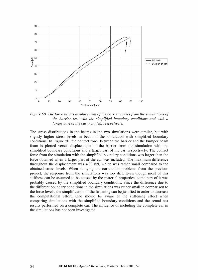
CHALMERS, Applied Mechanics, Master’s Thesis 2010:52 54
Figure 50. The force versus displacement of the barrier curves from the simulations of
the barrier test with the simplified boundary conditions and with a
larger part of the car included, respectively.
The stress distributions in the beams in the two simulations were similar, but with slightly higher stress levels in beam in the simulation with simplified boundary conditions. In Figure 50, the contact force between the barrier and the bumper beam foam is plotted versus displacement of the barrier from the simulation with the simplified boundary conditions and a larger part of the car, respectively. The contact force from the simulation with the simplified boundary conditions was larger than the force obtained when a larger part of the car was included. The maximum difference throughout the displacement was 4.33 kN, which was rather small compared to the obtained stress levels. When studying the correlation problems from the previous project, the response from the simulations was too stiff. Even though most of this stiffness can be assumed to be caused by the material properties, some part of it was probably caused by the simplified boundary conditions. Since the difference due to the different boundary conditions in the simulations was rather small in comparison to the force levels, the simplification of the fastening can be justified in order to decrease the computational effort. One should be aware of the stiffening effect when comparing simulations with the simplified boundary conditions and the actual test results performed on a complete car. The influence of including the complete car in the simulations has not been investigated.

CHALMERS, Applied Mechanics, Master’s Thesis 2010:52 55
7 Material specific investigation
In order be able to predict the behaviour of components made of short fibre reinforced polyamide 6, it is essential to know how the material behaves under certain conditions. Further investigation on material properties and quality has been included in the project, since reliable results could not be obtained from only the rather small number of physical experiments performed on beams. Additional tests on specimens out of beam material were performed. In this section, the influence from moisture is presented, followed by the influence from strain rate and temperature. Finally, the material quality in the beams is described.
7.1 Influence from moisture on the modulus of elasticity
It is known that moisture works as a softener in polyamide, see Section 4.4. It is however unknown how large impact the moisture content has on the mechanical properties of the material. The absorption and desorption of moisture are rather slow processes. Even though the beams were not easily dried, see Section 5.1, the moisture can still be the reason to part of the correlation problem in the previous project. Relative long time went by between the material testing, where the material parameters for designing the beams were determined, and the actual crash tests. There is reason to believe that the moisture content in the material varied between these different occasions.
Tensile tests were made in order to determine how the modulus of elasticity varies with moisture content. Four specimens from a crash box from beam 27 were used for the tests. The modulus of elasticity for each of the specimens was measured in a tensile test with an extensometer at a strain rate of 1 mm/min for four different moisture contents. The two lowest moisture contents for each specimen were obtained by drying the specimens at 150 ˚C for 3 and 9 hours respectively. The highest moisture content was obtained by placing the specimens in water for 12 hours. The intermediate moisture content, just above 1 %, was the moisture content corresponding to equilibrium with the surrounding at room temperature. The modulus was calculated between forces of 100 and 200 N, which correspond to low strains. The specimens were not pulled further to fracture and could therefore be tested again. The main advantage of testing the same specimens several times is that the fibre content and fibre orientation are kept constant for different moisture contents. One disadvantage is the risk of damage in the specimens during the tensile tests, which could affect the performance in the upcoming tests. Another drawback is that the tensile strength and strain at fracture will not be determined, even though they are of interest. However, the impact on the modulus of elasticity may indicate the magnitude of relevance of the moisture content and the need of further investigation including tensile strength and strain at fracture. The modulus of elasticity versus moisture content can be seen in Figure 51. As expected the modulus decreases with increasing moisture content. An increase in moisture content from around 0.05 % to just above 2.15 % leads to a decrease in modulus of elasticity of between 0.7 and 1.2 GPa.

CHALMERS, Applied Mechanics, Master’s Thesis 2010:52 56
Figure 51. The modulus of elasticity as a function of the moisture content in the
specimens. Each of the series corresponds to a specimen.
7.2 Influence from strain rate and temperature on the
modulus of elasticity
According to some literature, (Mouhmid et al., 2006), the strain rate dependence for short glass fibre reinforced PA66 at low strain rates is small. This was also the case in the tests made in the previous project, where the bumper beam was developed. Tests were then performed at two strain rates, 5 and 500 mm/min, but both were low compared to the actual crash test situation. However, in the performed tests in this project, a stiffening effect can be seen, see Section 5.2. In order to try to determine the strain rate dependence of the material, additional tensile tests at different strain rates were performed at AdManus Materialteknik. Also, tensile tests for different temperatures were performed.
The modulus of elasticity was measured with an extensometer for four different specimens from a crash box from beam 27. The modulus was measured between forces of 100 and 200 N, which corresponds to low strains, in each tensile test. Only the modulus of elasticity was determined, so the specimens were not tested to fracture and could be tested several times. This was desired since it assures that the fibre content and fibre orientation were the same for all the different strain rates, as for the tests with different moisture contents described in the previous subsection. It would be desirable to determine the tensile strength and strain at fracture as well, but as for the moisture content, the modulus of elasticity is assumed to indicate the magnitude of the impact from strain rate and temperature. First, the specimens were tested in tensile tests with six different deformation velocities, namely 100, 10, 1, 0.1, 0.01 and 0.001 mm/min which correspond to strain rates from 0.021 to 0.00000021 s-1. Second, the same specimens were tested tempered to four different temperatures, namely -5,

CHALMERS, Applied Mechanics, Master’s Thesis 2010:52 57
10, 23 and 45 ˚C, at a deformation rate of 1 mm/min. The strain was measured between the grips, due to the difficulties fastening the extensometer when trying to isolate the specimens to prevent a temperature change. Constant moisture content can not be assured with the available equipment, but the tests are performed in a series so there is reason to believe that the moisture content is more or less constant.
The strain measurements from the tensile tests done at the two highest strain rates seem to be uncertain, see Figure 52. In order to obtain a reasonable modulus of elasticity, the slope of a linear least square error line in a stress versus strain plot from the test was used.
Figure 52. A stress versus strain curve for the first specimen tested at a strain rate of
100 mm/min with a solid line indicating the trend from the test. The
stress is in GPa for direct calculation of the modulus of elasticity.
The measurements from the four lowest rates were better and the modulus of elasticity could be calculated as intended between forces of 100 and 200 N without large uncertainties. For the four lowest rates, the modulus of elasticity increases with increased strain rate, as expected, see Section 4.3. The increase in modulus is linear when the modulus is plotted versus the logarithm of the strain rate, see Figure 53. For strain rates above 1 mm/min, the modulus does not seem to further increase with the strain rate. It seems reasonable, that there is a knee point in the curve, above which the modulus does not increase as much with increased strain rate as below. The thin line in Figure 53, is an extrapolation of the linear increase seen for lower strain rates. The extrapolation is done up to strain rates corresponding to the ones present in the dynamic testing of the bumper beam, around 2 s-1. If this trend would be valid, the modulus of elasticity would be so high that the beam would respond extremely stiff at high strain rates, which has not been observed in the performed tests. However, one should be aware of the uncertainties in the strain measurements at the higher strain rate tensile tests performed here. There may still exist a small hardening effect for

CHALMERS, Applied Mechanics, Master’s Thesis 2010:52 58
strain rates above 1 mm/min, even though the modulus seems to not increase further in these tests.
Figure 53. The modulus of elasticity versus the logarithm of strain rate. The mean
value of the modulus of the four specimens is used at each strain rate.
The thin line indicates the linear relation found for lower strain rates
extrapolated to higher strain rates.
The results from the tensile tests with tempered specimens can be seen in Figure 54. Note that the rather low values of the modulus of elasticity are due to the fact that the strain was measured over the entire specimen, instead of with an extensometer. The tests at different temperatures are however still comparable and should indicate the temperature dependence. As expected, the modulus of elasticity decreases with increased temperature. The results from the tests performed at specimens with a temperature of 10 ˚C are not following the expected trend. The specimens were tested once again at this temperature, but similar results were obtained once more.
It is known that the strain rate dependence of a polymer is different below and above its glass temperature, see Section 4.3. The glass temperature of PA6 is between 50 and 60 ˚C, but may be lowered due to the moisture content. According to the coupling between temperature and strain rate, if the knee point is present when the modulus of elasticity is plotted versus temperature, that might indicate that there exists a knee point on the modulus versus strain rate curve as well.

CHALMERS, Applied Mechanics, Master’s Thesis 2010:52 59
Figure 54. The modulus of elasticity as a function of temperature. Each series
corresponds to a specimen. The relative low modulus of elasticity is due
to the fact that the strain was measured between the grips, not with an
extensometer, but the trend should be representative.
7.3 Material quality
The fibre orientation in the bumper beam is of interest, since it was not clear whether the compression moulding induced a layered structure. The fibre orientation was investigated at AdManus Materialteknik and was, as expected, not completely random. Some fibre orientation could be seen in the different parts of the beam. Since it is not known how the melt filled the form, it is not possible to draw any further conclusions on the relation between the fibre orientation and mould filling. In Figure A. 15, the fibre orientation in the surface of a polished piece from the front side of a bumper beam can be seen. The fibre orientation seems to be more or less random. This does not necessary indicate a random orientation throughout the thickness of the wall. A random orientated skin layer is also present for injection moulded part due to the rapid cooling when the melt reaches the mould, see Section 4.2.
The fibre length distribution is of importance in order to know how efficient the reinforcement can be, see Section 4.1.2. The fibre length distribution in the beams has been unknown, since the manufacturing included milling the fibres. The original length of the fibres was 12 mm. The fibre length distribution in some parts of the beams has been investigated at AdManus Materialteknik. Fibres with lengths very close to zero were neglected, since they were very many and do hardly contribute to the reinforcement. The fibre length distributions in the front side, the rear side and the crash boxes can be seen in Figure A. 12 to Figure A. 14, in Appendix A. The main fraction of the fibres was less than 1 mm and only a few fibres were longer than 1 mm. The distribution was similar in the front side, rear side and the crash boxes.

CHALMERS, Applied Mechanics, Master’s Thesis 2010:52 60
These results were expected and the distribution was similar to a typical fibre length distribution in short fibre reinforced injection moulded parts, (Hull, Clyne, 1996).
One of the major issues concerning the material properties in this project is the knee point in the stress-stain curves obtained in the tensile tests until fracture. It is not clarified whether yielding occurs or not. The yield stress for neat PA6, of the kind used in the beams, is normally 90 MPa in the dry state. For the conditioned polymer, it is instead 45 MPa. The stress levels where the knees occur in the tensile tests are low compared to these values. When the polymer matrix in a short fibre composite reaches its yield stress, the load can not be transferred to the fibres in an efficient way. After yielding, the polymer undergoes large deformations. Since the composite material was quite stiff also after the knee point, the following deformation was not very large. Another possible reason to the knee point is that the fibre-matrix bonding is not strong enough, i.e. it can correspond to a point where some fibres debond from the matrix.
Defects, such as pores and unwetted fibres, also affect the final properties of the material. The quality has been investigated at AdManus Materialteknik. Pores were present in the material, see Figure A. 16 in Appendix A. In the thicker walls of the beam, more pores were present compared to the thinner ones. One can note the difference when comparing cross sections from different parts of the beam. The crash boxes have the thickest walls and they contain most pores. The front side wall is of intermediate thickness and the rear side has the thinnest wall. The difference in pore content is expected, since larger dimensions, and the thereby larger volume of material, gives more shrinkage when the material cool down after the manufacturing. When the surface regions solidify faster than the inner parts, pores may form in the interior region, see the bottom three pictures in Figure A. 16 in Appendix A.

CHALMERS, Applied Mechanics, Master’s Thesis 2010:52 61
8 Results
The quasi static behaviour of the beams, without steel reinforcements, adhesive joints and bumper beam foam and with well defined loading and boundary conditions, could be simulated satisfactory by assuming isotropic material. A bilinear material model was used in order to capture the material behaviour in the tensile tests made on specimens from the tested beams.
No failure criterion was used in the material model, since the fracture mechanisms of the material were not known in detail. Instead, the material at the location where fracture was expected from the test was studied. A critical strain was used, based on the maximum principal strain and tension in the material, see Section 4.1.1 and Equation (5.1), and turned out to give a reasonable fracture prediction. The critical strain at fracture was a little less than 2 % for beam 10, 29, 27 and 26. For beam 18, the critical strain was 2.6 %, but that seems reasonable due to the fact that the glass fibre fraction was lower in that beam.
When performing two tests where the aim was to keep all parameters but the strain rate constant, a stiffening effect could be seen in the impact test. This indicated that the material is strain rate dependent. The stiffening effect is estimated from comparing the force versus displacement curves from the quasi static and the impact test, see Figure 33. The actual effect can be assumed to be even bigger, since the material in the beam in the impact test turned out to have a lower modulus of elasticity than the beam in the quasi static test.
In order to determine the strain rate dependence of the beam material, tensile tests at different strain rates were performed. Since no equipment for high strain rate testing was available, only strain rates low compared to the ones in the actual dynamic tests were used. A strain rate hardening could be seen. The modulus of elasticity increased linearly with the logarithm of the strain rate for strain rates below 0.00021 s-1. A knee point is present in the curve and the modulus of elasticity is more or less constant above that point. In addition tensile test at four different temperatures where performed and as expected the modulus of elasticity increased with decreasing temperature. The results from tests performed at 10 °C were unfortunately not following the trend of the other results. The reason to this could not be clarified within this project.
The simulations of the test performed on a beam with adhesive steel reinforcements, did not correlate well to the actual test. The quality of the adhesive joint and the properties of the adhesive could not be assured. The first detachment of the adhesive did not occur in the same region in the simulation and the test. The adhesive on the front side of the beam detaches near the circular impactor quite early in the tests. The quality of the adhesive joint may be poor there. A simulation where the adhesive was removed in that area gave better correlation between the force versus displacement curves from test and simulations.
The updated simulations of the crash tests in the previous project with the lower pendulum and the barrier with a bilinear material model, gave better correlation between the force versus displacement curves from the test data and the simulations. The more accurate material properties used in the updated simulations, improved the
CHALMERS, Applied Mechanics, Master’s Thesis 2010:52 62
correlation much. The forces versus displacement curves from the simulations of the high pendulum test do not correlate with the test data. The curves do not have the same shape. However, the curve from the updated simulation is located nearer the actual test data.
When a larger part of the car was modelled in the simulations, instead of just modelling the ends of the bolts through the crash boxes as fixed in space, the result was a less stiff response. The larger part of the car is a better model of the actual crash test, where a complete car was tested. The response in the simulations of crash tests, where the simplified boundary conditions are used, can therefore be assumed to be a bit too stiff.
The glass fibre fraction of the beams turned out to be much lower than prescribed. Instead of 37 or 45 wt% glass fibre the beams tested in this project had glass fibre contents in the range from 16.8 to 32.8 wt%. Tensile tests performed on specimens with different moisture content showed that the modulus of elasticity decreased with increasing moisture content. A increase in moisture content from just above zero to around 2 wt% lead to an decrease of the modulus of between 0.7 and 1.2 GPa, see Figure 51.
The fibre orientation was not completely random. At some locations some directions had an increased fibre orientation; these could not be related to the mould filling since it is unknown how the melt fills the mould. A somewhat layered structure could be seen and a random surface skin could be seen on the front side of a beam. The fibre length distribution turned out to be similar in the front side, the rear side and the crash boxes. A large fraction of the glass fibres in the beams are less than 1 mm and many have a length very close to zero.
CHALMERS, Applied Mechanics, Master’s Thesis 2010:52 63
9 Conclusions
The main part of the differences obtained between the crash tests and the simulations in the previous project was due to invalid material properties. The material used when designing the beam and in the simulations was much stiffer than the actual material in the produced and tested beams. After further investigation of the material quality, it turned out that the actual glass fibre fraction in the beams was much lower than expected. When studying the glass fibre fraction and the stiffness of the material, it can be concluded that a larger fraction do not always correspond to a higher modulus of elasticity. There is reason to believe that the adhesion between the matrix and the fibres not always is of good quality. Pores and other defects were also present in the beams. It is of big importance for the correlation between the tests and simulations that the material quality is trustworthy, which was not the case for the bumper beam prototypes.
When using a bilinear material model, with properties valid for the specific beam, the assumption of isotropic material behaviour gives a simulation which shows a satisfactory correlation with the test. Even though the material is not isotropic, the orientation effects in the beams seemed to be small enough to be neglected. According to literature, see Section 4.2, the fibre orientation effects, due to injection moulding, are small for thick components and low injection velocities. The thicknesses of the bumper beam are large compared to the usual dimensions of injection moulded parts. Also, the velocity of the melt as it fills the mould is low compared to the injection velocities used for injection moulding.
The short fibre reinforced PA6 in the bumper beams has some strain rate dependence. This gives a stiffening effect when loading the beam dynamically. This effect is estimated to be between 20 to 30 % from the force versus displacement curves from tests performed on bumper beams. Tensile tests at various strain rates show a hardening effect when the strain rate is increased, for low strain rates. The increase seems to decline at a strain rate around 0.00021 s-1. Due to uncertainties in the measurements, only limited conclusions can be drawn about the magnitude of the strain rate dependence above that level. The decline in strain rate sensitivity seems reasonable when studying the principal illustration of modulus as a function of strain rate, see Figure 12 (note that strain increases to the left). Since the glass transition temperature varies with moisture content, it was not known whether the material in the specimens was above or under the glass transition temperature at the test occasion. The strain rate dependence is larger under the glass transition temperature than above, see Section 4.3. It is not likely that there exists a transition from isothermal to adiabatic behaviour in this material under the strain rate corresponding to low speed crashes, see Section 4.3.
The stiffness of the material also increases with lowered temperature, as expected. In the principal illustration of the variation of the modulus of elasticity with temperature in Figure 12, it can be seen in the range around the glass transition temperature is the temperature range where the temperature sensitivity is largest. In Figure A. 17, curves for the neat PA6 of the type used in the beams are found. The range with a large sensitivity can be seen to shift towards lower temperatures for the conditioned state compared to the dry. It could not be determined exactly how the glass transition temperature varies with the moisture content but it seems reasonable that the tested

CHALMERS, Applied Mechanics, Master’s Thesis 2010:52 64
temperature range is located under the glass transition temperature. The resulting curves should then correspond to the first convex part of the principal illustration, see Figure 12. In some of the studied literature, (Wang et al., 2002), (Mouhmid et al., 2006), the modulus of elasticity seemed to continue to increase with decreased temperature and no decline in the sensitivity could be seem. No temperatures under 20 ˚C were tested and the resulting curves do most likely correspond to the concave second part of the principal illustration. It is relevant to note that the moisture in the bumper beam may lower the glass transition temperature. That may result in that the beam will be used in the temperature range around the transition temperature. The behaviour of the beam can then be affected to a larger extent.
The moisture content does not only change the glass transition temperature but the stiffness of the material. It is of importance to investigate under which circumstances the material is supposed to be used before the actual parameters of the material can be determined. One also has to note that the polyamide is dry when newly manufactured.
One of the major concerns in order to predict the failure of the bumper beams is a valid failure criterion. A quite simple, and possibly also adequate, measure used here is the critical strain, at which crazing may occur. The critical strain is found to be somewhat dependent on the glass fibre content but normally in the range from a little less than 2 up to 2.6 %. The maximum principal strain was used for the evaluation, but if the effective strain was used instead, the same trend was present but with somewhat lower values. If the maximum principal stresses from the fracture locations are compared to the tensile strengths from the tensile tests to fracture, the obtained stress levels in the beams are much lower, except for beam 18. The tensile tests are performed at specimens from the walls and most fractures occur in junctions, where the material properties may be different. One must be aware that crazing must not occur prior to the fracture in short fibre composites and that other fracture mechanisms may be critical.
CHALMERS, Applied Mechanics, Master’s Thesis 2010:52 65
10 Discussion and recommendations
The main reasons for the correlation problems in the previous project have been investigated and conclusions of their importance can be drawn, but there are some drawbacks concerning the testing within this project. Only a few beams were available for testing, leading to a very limited number of tests. More tests with corresponding simulations, especially dynamic ones, would have been preferable to obtain reliable results. Additional measurements were made to verify the stiffness of the test rig used for the quasi static experiments. The uncertainties due to the fact that the rig is not completely stiff are very small in comparison to other uncertainties within the project and can therefore be neglected see Appendix E. The tracking of points in the films from the tests did unfortunately not give any useful information. The reason is however not known, see Appendix E.
There are unfortunately some sources of error concerning the material testing. Only 6 or 8 specimens were taken from each beam for the tensile tests and a large variation was obtained. The material quality may vary a lot from specimen to specimen. The large variation was handled by using a mean value to establish properties for the material model. A safety factor or a value which a large fraction of the test results exceeds should instead have been used, if the aim would have been to design a new component or determine if a structure will stand a certain load situation. The specimens were sawed out from the beam so it was impossible to make them all equal and of such good quality as one could wish. Specimens could only be taken in the front and rear side of the beam and in the crash boxes and not in the locations where fracture several times did occur, like the junctions between the walls and the supporting walls. An investigation on the fracture mechanisms of the material is also necessary to establish a reliable fracture criterion.
The influence of the moisture content on the glass transition temperature must be further investigated as well as the material properties at different temperatures. This is of great importance since it is crucial to predict the properties in application, at the level of moisture content and temperature present. Also, the behaviour of the material at high strain rates should be further tested with high strain rate tensile test equipment.
Further investigation of the fibre orientation obtained due to the compression moulding is of great importance, both in order to verify the assumption of isotropic material behaviour as well as to learn more about how the material fractures with respect to the fibre orientation. Simulation softwares for compression moulding would be a great aid and would make it possible to refine the simulations with local properties according to the fibre distribution.
The main reason to the unsatisfactory correlation between experiments and simulations for the bumper beam has been that the material did not have the expected properties. This was mainly due to the manufacturing of the beams. For future work in similar projects, it is strongly recommended to assure the material properties and quality in the prototypes. Further investigation on the influence from the manufacturing process on the material properties are recommended in order to make sure that the properties of the components can be predicted. It is also important to assure that the manufacturing process gives the same result time after time. In compression moulding, it includes a precise portioning and placement of the charge.

CHALMERS, Applied Mechanics, Master’s Thesis 2010:52 66
For the bumper beam concept, short glass fibre reinforced PA6 might not be the right choice before the above mentioned tasks has been solved. The adhesive joints should be reconsidered since it caused further complications. There are other possible ways to reinforce polymers, such as steel wires moulded together with the component.

CHALMERS, Applied Mechanics, Master’s Thesis 2010:52 67
References
Bernasconi, A., Davoli, P., Basile, A., Filippi, A., Effect of fibre orientation on the fatigue behaviour of a short glass fibre reinforced polyamide-6, International Journal
of Fatigue 29 (2007), p. 199-208, Elsevier Ltd., 2006
Callister, W. D. Jr., Materials Science and engineering, An introduction, 6th edition, ISBN: 0-471-22471-5, John Wiley & Sons, Inc., 2003
Cook, R. D., Malkus, D. S., Plesha, M. E., Concepts and Applications of Finite
Element Analysis, 3rd edition, ISBN: 0-471-84788-7, John Wiley & Sons, Inc., USA, 1989
Crisfield, M. A., Non-linear Finite Element Analysis of Solids and Structures, Volume
2: Advanced Topics, ISBN: 0 471 95649 X, John Wiley & Sons Ltd, England, 1997
De Monte, M., Moosbrugger, E., Quaresimin, M., Influence of temperature and thickness on the off-axis behaviour of short glass fibre reinforced polyamide 6.6 – Quasi-static load, Composites: Part A (2010), Elsevier Ltd., 2010.
De Monte, M., Moosbrugger, E., Jaschek, K., Quaresimin, M., Multiaxial fatigue of a short glass fibre reinforced polyamide 6.6 – Fatigue and fracture behaviour, International Journal of Fatigue 32 (2010), p. 17-28, Elsevier Ltd., 2009
Hallquist, J. O., LS-DYNA Theory Manual, ISBN: 0-9778540-0-0, Livermore Software Technology Corporation, 2006
Hull, D., Clyne, T. W., An Introduction to Composite Materials, 2nd edition, ISBN: 0-521-38190-8, Cambridge University Press, 1996
Hult, J., Bjarnehed, H., Styvhet och styrka, Grundläggande kompositmekanik, (Stiffness and strength, Fundamental mechanics of composites, in Swedish), ISBN: 91-44-38101-8, Studentlitteratur, Lund, 1993
Kelly, A., Zweben, C., (editors), Comprehensive Composite Materials, ISBN: 978-0-08-042993-9, Volume 1: p. 377-401, Volume 2: p. 151-197, 291-331, Elsevier Science Ltd, 2000
Klason, C., Kubát, J., Platser – Materialval och materialdata, (Plastics – Material Choise and Material Data, in Swedish), ISBN: 91-7548-618-0, Industrilitteratur, 5th edition, 2004
LS-DYNA Keyword User’s Manual, Version 971, Volume I, ISBN: 0-9778540-2-7, Livermore Software Technology Corporation, 2007
LS-DYNA Keyword User’s Manual, Version 971, Volume II, Material Models, ISBN: 0-9778540-3-5, Livermore Software Technology Corporation, 2007
McCrum, N. G., Buckley, C. P., Bucknall, C. B., Principles of Polymer Engineering, 2nd edition, ISBN: 978-0-19-856526-0, Oxford Science Publications, (1997), 2007
CHALMERS, Applied Mechanics, Master’s Thesis 2010:52 68
Mouhmid B., Imad, A., Benseddiq, N., Benmedakhène, S., Maazouz, A., A study of the mechanical behaviour of a glass fibre reinforced polyamide 6,6: Experimental investigation, Polymer Testing 25 (2006), p. 544-552, Elsevier Ltd., 2006.
Mulliken, A. D., Mechanics of Amorphous Polymers and Polymer Nanocomposites during High Rate Deformation, Ph.D., Massachusetts Institute of Technology, 2006
Piggott, M. R., Load Bearing Fibre Composites, 2nd edition, ISBN: 9780306475917, Kluwer Academic Publishers, Boston, 2002.
Schoßig, M., Bierögel, C., Grellmann, W., Mecklenburg, T., Mechanical behaviour of glass-fibre reinforced thermoplastic materials under high strain rates, Polymer Testing
27 (2008), p. 893-900, Elsevier Ltd., 2008
Sundström, B. (ed.), Handbok och formelsamling i hållfasthetslära, (Handbook and formulary in strength of mechanics, in Swedish), Instutitionen för hållfasthetslära KTH, Södertälje, 1998
Wang, Z., Zhou, Y., Mallick, P. K., Effects of Temperature and Strain Rate on the Tensile Behavior of Short Fiber Reinforced Polyamide-6, Polymer Composites, Vol. 23, No. 5, 2002
Internet resources
CADPRESS – Compression Simulation software, The Madison group, http://www.madisongroup.com/engineering/cadpress.html, (accessed 2010-05-21)
Campus Plastics, Computer Aided Material Preselection by Uniform Standards, http://www.campusplastics.com/campus/datasheet/Ultramid%C2%AE+B3S/BASF/20/caf8ea95, (accessed 2010-07-29)
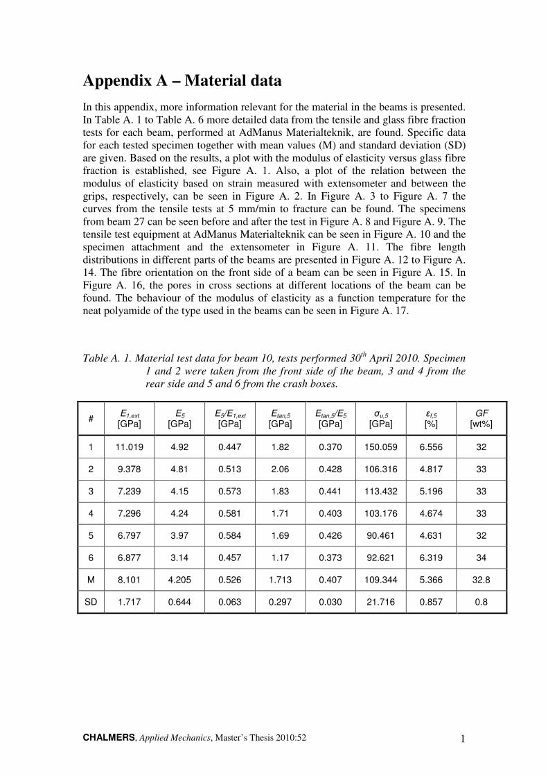
CHALMERS, Applied Mechanics, Master’s Thesis 2010:52 1
Appendix A – Material data
In this appendix, more information relevant for the material in the beams is presented. In Table A. 1 to Table A. 6 more detailed data from the tensile and glass fibre fraction tests for each beam, performed at AdManus Materialteknik, are found. Specific data for each tested specimen together with mean values (M) and standard deviation (SD) are given. Based on the results, a plot with the modulus of elasticity versus glass fibre fraction is established, see Figure A. 1. Also, a plot of the relation between the modulus of elasticity based on strain measured with extensometer and between the grips, respectively, can be seen in Figure A. 2. In Figure A. 3 to Figure A. 7 the curves from the tensile tests at 5 mm/min to fracture can be found. The specimens from beam 27 can be seen before and after the test in Figure A. 8 and Figure A. 9. The tensile test equipment at AdManus Materialteknik can be seen in Figure A. 10 and the specimen attachment and the extensometer in Figure A. 11. The fibre length distributions in different parts of the beams are presented in Figure A. 12 to Figure A. 14. The fibre orientation on the front side of a beam can be seen in Figure A. 15. In Figure A. 16, the pores in cross sections at different locations of the beam can be found. The behaviour of the modulus of elasticity as a function temperature for the neat polyamide of the type used in the beams can be seen in Figure A. 17.
Table A. 1. Material test data for beam 10, tests performed 30th
April 2010. Specimen
1 and 2 were taken from the front side of the beam, 3 and 4 from the
rear side and 5 and 6 from the crash boxes.
# E1,ext
[GPa]
E5 [GPa]
E5/E1,ext [GPa]
Etan,5 [GPa]
Etan,5/E5 [GPa]
σu,5 [GPa]
εf,5 [%]
GF [wt%]
1 11.019 4.92 0.447 1.82 0.370 150.059 6.556 32
2 9.378 4.81 0.513 2.06 0.428 106.316 4.817 33
3 7.239 4.15 0.573 1.83 0.441 113.432 5.196 33
4 7.296 4.24 0.581 1.71 0.403 103.176 4.674 33
5 6.797 3.97 0.584 1.69 0.426 90.461 4.631 32
6 6.877 3.14 0.457 1.17 0.373 92.621 6.319 34
M 8.101 4.205 0.526 1.713 0.407 109.344 5.366 32.8
SD 1.717 0.644 0.063 0.297 0.030 21.716 0.857 0.8
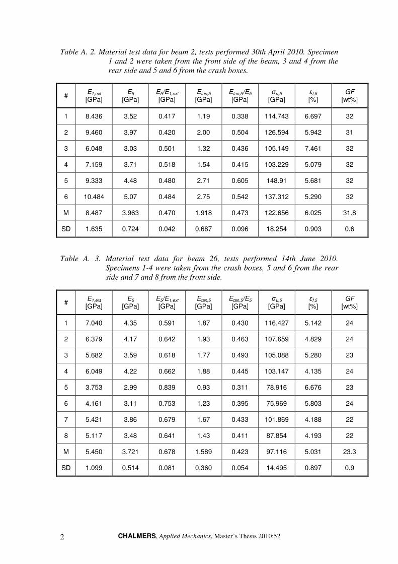
CHALMERS, Applied Mechanics, Master’s Thesis 2010:52 2
Table A. 2. Material test data for beam 2, tests performed 30th April 2010. Specimen
1 and 2 were taken from the front side of the beam, 3 and 4 from the
rear side and 5 and 6 from the crash boxes.
# E1,ext
[GPa]
E5 [GPa]
E5/E1,ext [GPa]
Etan,5 [GPa]
Etan,5/E5 [GPa]
σu,5 [GPa]
εf,5 [%]
GF [wt%]
1 8.436 3.52 0.417 1.19 0.338 114.743 6.697 32
2 9.460 3.97 0.420 2.00 0.504 126.594 5.942 31
3 6.048 3.03 0.501 1.32 0.436 105.149 7.461 32
4 7.159 3.71 0.518 1.54 0.415 103.229 5.079 32
5 9.333 4.48 0.480 2.71 0.605 148.91 5.681 32
6 10.484 5.07 0.484 2.75 0.542 137.312 5.290 32
M 8.487 3.963 0.470 1.918 0.473 122.656 6.025 31.8
SD 1.635 0.724 0.042 0.687 0.096 18.254 0.903 0.6
Table A. 3. Material test data for beam 26, tests performed 14th June 2010.
Specimens 1-4 were taken from the crash boxes, 5 and 6 from the rear
side and 7 and 8 from the front side.
# E1,ext
[GPa]
E5 [GPa]
E5/E1,ext [GPa]
Etan,5 [GPa]
Etan,5/E5 [GPa]
σu,5 [GPa]
εf,5 [%]
GF [wt%]
1 7.040 4.35 0.591 1.87 0.430 116.427 5.142 24
2 6.379 4.17 0.642 1.93 0.463 107.659 4.829 24
3 5.682 3.59 0.618 1.77 0.493 105.088 5.280 23
4 6.049 4.22 0.662 1.88 0.445 103.147 4.135 24
5 3.753 2.99 0.839 0.93 0.311 78.916 6.676 23
6 4.161 3.11 0.753 1.23 0.395 75.969 5.803 24
7 5.421 3.86 0.679 1.67 0.433 101.869 4.188 22
8 5.117 3.48 0.641 1.43 0.411 87.854 4.193 22
M 5.450 3.721 0.678 1.589 0.423 97.116 5.031 23.3
SD 1.099 0.514 0.081 0.360 0.054 14.495 0.897 0.9
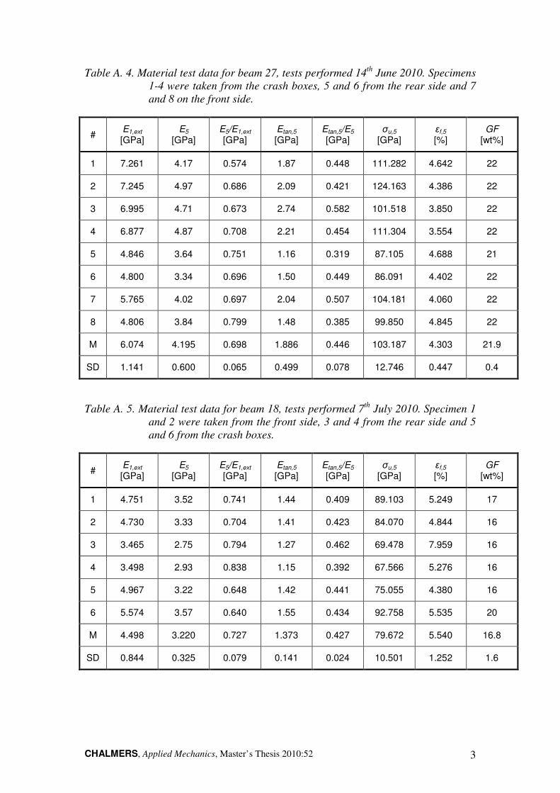
CHALMERS, Applied Mechanics, Master’s Thesis 2010:52 3
Table A. 4. Material test data for beam 27, tests performed 14th
June 2010. Specimens
1-4 were taken from the crash boxes, 5 and 6 from the rear side and 7
and 8 on the front side.
# E1,ext
[GPa]
E5 [GPa]
E5/E1,ext [GPa]
Etan,5 [GPa]
Etan,5/E5 [GPa]
σu,5 [GPa]
εf,5 [%]
GF [wt%]
1 7.261 4.17 0.574 1.87 0.448 111.282 4.642 22
2 7.245 4.97 0.686 2.09 0.421 124.163 4.386 22
3 6.995 4.71 0.673 2.74 0.582 101.518 3.850 22
4 6.877 4.87 0.708 2.21 0.454 111.304 3.554 22
5 4.846 3.64 0.751 1.16 0.319 87.105 4.688 21
6 4.800 3.34 0.696 1.50 0.449 86.091 4.402 22
7 5.765 4.02 0.697 2.04 0.507 104.181 4.060 22
8 4.806 3.84 0.799 1.48 0.385 99.850 4.845 22
M 6.074 4.195 0.698 1.886 0.446 103.187 4.303 21.9
SD 1.141 0.600 0.065 0.499 0.078 12.746 0.447 0.4
Table A. 5. Material test data for beam 18, tests performed 7th
July 2010. Specimen 1
and 2 were taken from the front side, 3 and 4 from the rear side and 5
and 6 from the crash boxes.
# E1,ext
[GPa]
E5 [GPa]
E5/E1,ext [GPa]
Etan,5 [GPa]
Etan,5/E5 [GPa]
σu,5 [GPa]
εf,5 [%]
GF [wt%]
1 4.751 3.52 0.741 1.44 0.409 89.103 5.249 17
2 4.730 3.33 0.704 1.41 0.423 84.070 4.844 16
3 3.465 2.75 0.794 1.27 0.462 69.478 7.959 16
4 3.498 2.93 0.838 1.15 0.392 67.566 5.276 16
5 4.967 3.22 0.648 1.42 0.441 75.055 4.380 16
6 5.574 3.57 0.640 1.55 0.434 92.758 5.535 20
M 4.498 3.220 0.727 1.373 0.427 79.672 5.540 16.8
SD 0.844 0.325 0.079 0.141 0.024 10.501 1.252 1.6

CHALMERS, Applied Mechanics, Master’s Thesis 2010:52 4
Table A. 6. Material test data for beam 30, tests performed 7th
July 2010. Specimen 1
and 2 were taken from the front side, 3 and 4 from the rear side and 5
and 6 from the crash boxes.
# E1,ext
[GPa]
E5 [GPa]
E5/E1,ext [GPa]
Etan,5 [GPa]
Etan,5/E5 [GPa]
σu,5 [GPa]
εf,5 [%]
GF [wt%]
1 8.480 4.41 0.520 2.05 0.465 99.145 4.575 30
2 9.259 6.20 0.670 2.65 0.427 141.113 4.413 31
3 9.001 2.09 0.232 1.97 0.943 110.357 5.950 30
4 6.582 5.54 0.842 2.05 0.370 110.269 3.986 31
5 9.348 5.73 0.613 2.18 0.380 151.539 5.680 31
6 10.388 5.45 0.525 2.09 0.383 136.524 5.198 30
M 8.843 4.903 0.567 2.165 0.495 124.824 4.967 30.5
SD 1.271 1.498 0.202 0.247 0.222 20.959 0.768 0.5
Figure A. 1. The modulus of elasticity, E1,ext, versus the weight fraction glass fibre in
each tested specimen.

CHALMERS, Applied Mechanics, Master’s Thesis 2010:52 5
Figure A. 2. The modulus of elasticity measured at 1 mm/min with an extensometer,
E1,ext, versus the modulus of elasticity measured in the tensile test to
fracture at 5 mm/min, E5.
Figure A. 3. The stress versus strain curves from the tensile tests to fracture at
5 mm/min for specimens from beam 29. The strain was measured over
the entire specimen.
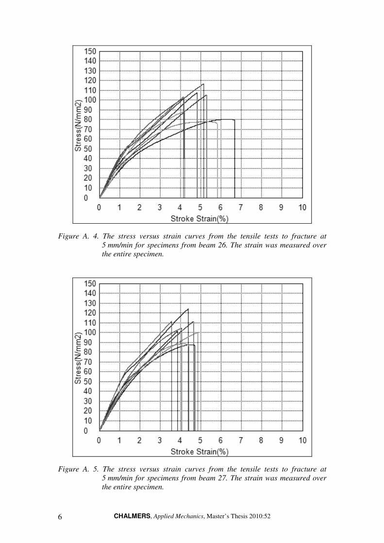
CHALMERS, Applied Mechanics, Master’s Thesis 2010:52 6
Figure A. 4. The stress versus strain curves from the tensile tests to fracture at
5 mm/min for specimens from beam 26. The strain was measured over
the entire specimen.
Figure A. 5. The stress versus strain curves from the tensile tests to fracture at
5 mm/min for specimens from beam 27. The strain was measured over
the entire specimen.
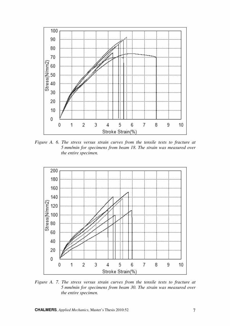
CHALMERS, Applied Mechanics, Master’s Thesis 2010:52 7
Figure A. 6. The stress versus strain curves from the tensile tests to fracture at
5 mm/min for specimens from beam 18. The strain was measured over
the entire specimen.
Figure A. 7. The stress versus strain curves from the tensile tests to fracture at
5 mm/min for specimens from beam 30. The strain was measured over
the entire specimen.

CHALMERS, Applied Mechanics, Master’s Thesis 2010:52 8
Figure A. 8. The specimens from beam 27 before the tensile tests.
Figure A. 9. The specimens from beam 27 after the tensile tests. It is desirable that the
probes fracture in the middle of the specimen, which is the case only for
the 5th
specimen.

CHALMERS, Applied Mechanics, Master’s Thesis 2010:52 9
Figure A. 10. The tensile test equipment at AdManus Materialteknik.
Figure A. 11. The specimen attachment in the grips (left) and the extensometer
mounted on the specimen (right). The measuring distance for the
extensometer is 25 mm.
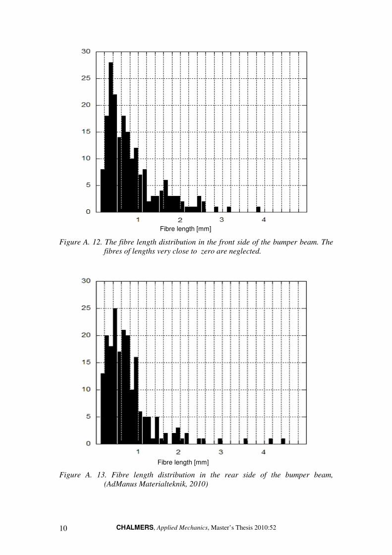
CHALMERS, Applied Mechanics, Master’s Thesis 2010:52 10
Figure A. 12. The fibre length distribution in the front side of the bumper beam. The
fibres of lengths very close to zero are neglected.
Figure A. 13. Fibre length distribution in the rear side of the bumper beam,
(AdManus Materialteknik, 2010)
Fibre length [mm]
Fibre length [mm]

CHALMERS, Applied Mechanics, Master’s Thesis 2010:52 11
Figure A. 14. The fibre length distribution in the crash box of the bumper beam,
(AdManus Materialteknik, 2010)
Figure A. 15. The fibre orientation on the front side of a bumper beam. The surface is
polished and studied in a microscope. (AdManus Materialteknik, 2010)
Fibre length [mm]

CHALMERS, Applied Mechanics, Master’s Thesis 2010:52 12
Figure A. 16. Pores in cross sections from different locations in beam A2; front side
(first row), rear side (second row, left), middle wall (second row, right)
and crash box (third and fourth row), (AdManus Materialteknik, 2010).

CHALMERS, Applied Mechanics, Master’s Thesis 2010:52 13
Figure A. 17. The modulus of elasticity versus temperature for neat PA6 of the kind
used in the beams, Ultramid® B3S, for the dry state (left) and the
conditioned state at 50 % RH (right), (Campus Plastics, 2010).
Table A. 7. Some properties for neat PA6 of the kind used in the beams, Ultramid®
B3S, for the dry state and conditioned state, at 50 % RH, (Campus
Plastics, 2010).
Dry Cond.
Modulus of elasticity [GPa] 3.4 1.2
Yield stress [MPa] 90 45
Melting temperature [˚C] 220 -
Glass transition temperature [˚C] 60 -
Density 1130 -
Table A. 8. Some properties for typical E-glass fibres, (Piggott, 2002).
Modulus of elasticity [GPa] 72
Tensile strength [MPa] 3400
Diameter [µm] 5-25
Maximum operation temperature [˚C] 550
Density [kg/m3] 2540

CHALMERS, Applied Mechanics, Master’s Thesis 2010:52 14
Appendix B – List of manufactured beams
In this appendix, a complete list of the manufactured beams in the previous project is given. Some beams were not kept after manufacturing and all beams could not be found at the time for this Master’s Thesis. The tool temperature is given for upper and lower mould part. The glass fibre fraction is the intended fraction in the production.
Table B. 1. A list of the manufactured prototype beams in the previous project. The
beams in bold style are the ones tested within this project.
# Weight [g]
Pressure [bar]
Glass fibre [wt%]
Tool temp. [˚C]
Thickness [mm]
Comments
A1 Tested, part of the beam is analyzed. Is at Ad Manus.
A2 Tested, part of the beam is analyzed. Is at Ad Manus.
A3 In the tool when it broke, is at Ljungby Komposit.
1 4398 150 37 50/60 Scraped after manufacturing.
2 4330 150 37 50/60 Scraped after manufacturing.
3 4480 150 37 50/60 Scraped after manufacturing.
4 4240 150 37 50/60 Scraped after manufacturing.
5 4334 150 37 50/60 Scraped after manufacturing.
6 4008 150 37 50/60 Scraped after manufacturing.
7 3832 150 37 50/60 Scraped after manufacturing.
8 3570 150 37 70/60 Scraped after manufacturing.
9 3726 150 37 70/60 Not tested, no adhesive/steel.
Is at Hovås Komposit.
10 3822 150 37 70/60 Tested in this project, 100428
11 3368 150 37 70/60 One of the crash boxes removed and tested.
12 3412 150 37 70/60 89.9 Missing
13 3676 150 37 70/60 90.4 Missing
14 3492 150 37 70/60 90.2 Tested in previous project
15 3442 150 37 70/60 90.6 Tested in previous project

CHALMERS, Applied Mechanics, Master’s Thesis 2010:52 15
16 3704 150 45 70/60 91.0 Tested in this project, 100426
17 3668 150 45 70/60 90.5
18 3496 150 45 70/70 90.6 Tested in this project, 100702
19 3738 150 45 70/70 90.5 Tested in previous project
20 3986 150 45 70/70 91.5 Scraped after manufacturing.
21 3824 150 45 70/70 91.4 Scraped after manufacturing.
22 3702 150 45 70/70 90.6 Missing
23 3748 150 45 70/70 91.0 Missing
24 3726 150 45 70/70 91.4 Scraped after manufacturing.
25 3554 150 45 70/70 90.0 Scraped after manufacturing.
26 3538 150 45 70/70 90.5 Tested in this project, 100528
27 3506 150 45 70/70 90.6 Tested in this project, 100519
28 3790 150 45 70/70 90.4 Missing
29 3766 150 45 70/70 89.9 Tested in this project, 100428
30 3772 150 45 70/70 90.0 Tested in this project, 100702
31 3656 150 45 70/70 90.5 Missing

CHALMERS, Applied Mechanics, Master’s Thesis 2010:52 16
Appendix C – Material models in LS-DYNA
The LS- DYNA material models used for the simulations of the performed experiments are briefly described in this appendix, (LS-DYNA Keyword User’s Manual, Version 971, Volume II, 2007).
MAT_001 *MAT_ELASTIC
The material model of type 1 is a model for an isotropic elastic material. It can be used for beam, shell and solid elements.
MAT_020 *MAT_RIGID
The material model of type 20 is a model of a rigid material. Parts made of this material are considered to belong to a rigid body.
MAT_024 *MAT_PIECEWISE_LINEAR_ELASTISITY
The material model of type 24 is a model for elasto-plastic materials with arbitrary stress versus strain curves. A load curve or a table with up to 8 stress and strain values can be defined to describe the behaviour. It is possible to establish a bilinear stress versus strain curve by defining a modulus of elasticity, yield stress and a tangent modulus. Also strain rate dependence can be defined.
MAT_185 *MAT_COHESIVE_TH
The material model of type 185 is a cohesive material model which can be used on
solid element types 19 and 20. A dimensionless separation measure, λ, is used
together with a trilinear traction-separation law, t(λ). The loading and unloading follows the same path. To describe the behaviour of a cohesive material, a peak
traction, σmax, must be defined. Additional, maximum separation lengths in the normal and tangential directions are defined. The shape of the traction versus deformation curve is described with scaled distances to peak traction, Λ1, beginning of softening, Λ2, and failure, Λfail, see Figure C. 1. The behaviour in the normal and tangential direction is different just due to the maximum separation lengths, NLS and TLS in the normal and tangential direction respectively. Apart from that the behaviour follows the same curve.

CHALMERS, Applied Mechanics, Master’s Thesis 2010:52 17
Figure C. 1. A typical traction, t(λ), versus deformation, λ, plot for an adhesive
material. The notation corresponds to MAT_COHESIVE_TH in
LS-DYNA, (LS-DYNA Keyword User’s Manual, Version 971, Volume II,
2007).

CHALMERS, Applied Mechanics, Master’s Thesis 2010:52 18
Appendix D – Notations for beam parts
In this appendix, the notation of different parts of the beam used throughout the report is clarified.
Figure D. 1. The notation of different parts of the beam used in the report.
Front side
Rear side
Middle walls
Crash box
Supporting walls
Joints
CHALMERS, Applied Mechanics, Master’s Thesis 2010:52 19
Appendix E – Uncertainties in simulations and tests
In this appendix the dynamic effects in the FE-simulations of the quasi static tests are discussed. Also, the investigations concerning the uncertainties in the physical quasi static tests are presented.
Dynamic effects in simulations of quasi static tests
Due to the time needed for the computations in the simulations, one want to use a rather high velocity for the prescribed motions in the quasi static tests. In order to make sure that the prescribed motion of the barrier and the circular impactor did not give rise to any dynamic effects in the simulations, simulations with different velocity of the impactors were made. These simulations were performed with the circular impactor but should be applicable for the simulations with the barrier as well. It can be seen in Figure E. 1, that the force versus displacement curve for the velocity 0.3 mm/ms coincide with the curve from the simulation with the velocity 0.03 mm/ms. This shows that there are no effects of the higher velocity used in the simulations of the quasi static tests. A simulation with a velocity of 3 mm/ms was made and it can be seen that the result still follows the same mean value, but that some oscillations were induced in the simulation.
Figure E. 1. The influence of displacement rate on the force versus displacement
curves from the simulations of the quasi static test with the circular
impactor. The simulation with the impact rate of 0.03 mm/ms was just
performed until a deformation of 30 mm, due to the long simulation
time.

CHALMERS, Applied Mechanics, Master’s Thesis 2010:52 20
Uncertainties concerning the testing
The displacements of the barrier and impactor presented throughout Section 5 are the measured displacements of the piston pushing the barrier or impactor forward during the test. A built in sensor is used for this, named GL-349.
Stiffness of the rig for quasi static tests
In order to see how stiff the rig is and how stiff it is fastened into the ground, some additional measurements were included at the last test session, where beam 18 and 30 were tested. A principal illustration of the additional measurements can be seen in Figure E. 2. In a perfectly stiff set up, GL-601 will equal GL-349 and GL-602 and GL-603 will equal zero.
Figure E. 2. A principal illustration of the test set up with the additional
measurements to determine the stiffness of the rig. The positive
direction for each displacement is indicated with arrows.
Once, the impactor was displaced without a beam mounted in the rig. The measurements from GL-601 and GL-349 were compared. During the movement of the impactor, GL-601 shows a larger displacement than GL-349. The difference increases with time and reaches its maximum, 1.24 mm, at the end of the movement. If the difference between GL-601 and GL-349 at each time were divided with the corresponding displacement measured in GL-349, the error was less than 2.5 % after some initial oscillations. Both GL-602 and GL-603 fluctuated around zero, with a maximum absolute value of 0.12 mm.
When beam 30 was tested, the displacement measured in GL-349 is larger than the one measure in GL-601 until the first fracture occurred and then GL-601 showed the larger displacement. The absolute value of the difference between GL-601 and GL-349 was increasing with increasing applied force. The difference between the two measurements for each time was divided with the corresponding displacement measured with GL-349, and the error seemed to be less than 4 %.
In the test on beam 30, the displacements in GL-602 were negative, corresponding to the wall moving towards the beam and the impactor. The displacement was not
CHALMERS, Applied Mechanics, Master’s Thesis 2010:52 21
proportional to the force; it first increased to a displacement of 0.5 mm in the negative direction, where it seemed to stabilize, with only small fluctuations. The displacements measured in GL-603 were positive, corresponding to that the test machine moved a bit backwards, which seems reasonable. The displacement seemed to be a function of the applied force. At a force of 30 kN the displacement was less than 0.7 mm. Assuming a worst case scenario, where the errors from GL-602 and GL-603 sum up, the error is still in the magnitude of 5 % of the total measured displacement measured with GL-349.
Film tracking
To be able to analyze the tests more in detail the tests were filmed. Prior to the tests, the beams were painted light gray to make cracks more visible. They were also provided with black and white tracking points to enable tracking in the film. All the junctions of the beam were tracked for all tests. Meta Post, version 6.3.1, was used for the tracking. Also the barrier or the impactor in each test was tracked. The time from first contact between the beam and the impactor and the corresponding displacement in the films, were compared to the measurements from the test occasion. There were uncertainties in these comparisons, due to the fact that it was not always obvious when the first contact occurred, neither in the tracked data from the film nor in the measurements. The contact time in the tracked data tended to be about 95 % of the contact time in the measurements. It is however unknown how exact the frame rate was after compression of the films. The displacement from first contact to fracture was shorter in the tracked data than in the test data, about 80 %. As a consequence of these differences, also the displacement velocities of the barrier and impactor in the quasi static tests as well as the velocity of the cart in the dynamic test were lower in the tracked films than in the test data.
The reason for the differences between the tracked data and the measured data is not known. For the correlation analyses the measured data from the test occasions were used, since it was assumed to be more accurate. A suspicion is that the camera was not placed far enough away from the beam were the distances were tracked. Also, there is a risk that the right pixel was not followed in the traction, so that an adjacent pixel is tracked. Such an error could lead to further uncertainties, but they should be small.