FACULTY OF ENGINEERING MULTIMEDIA UNIVERSITYfoe.mmu.edu.my/lab/lab sheet/LABSHEET TRIM2...

ETN 3096: Digital Signal Processing

2013/2014 1

FACULTY OF ENGINEERING MULTIMEDIA UNIVERSITY

LAB SHEETS

ETN 3096

DIGITAL SIGNAL PROCESSING TRIMESTER 2 (2013/2014)

DSP1: Introduction to DSP with Matlab

DSP2: Design of a Digital Filter with Matlab

(plus Demo on DSP Starter Kit)


2013/2014 2

Introduction to the Digital Signal Processing Labs

Students should develop the habit to read user manuals before using any product (software,

hardware or technical), and that online manuals and/or tutorials can easily be found with the use of

any search engine.

The purpose of the "Digital Signal Processing" labs is not to spend a lot of time just working out

theoretical results or following blindly some very specific instructions. The purpose is to give some

hands-on experience to the student by letting him "play around" with a number of basic signal

processing routines, and so develop a certain intuition about digital signal processing.

The expected result is that the student understands what he/she is doing and why he gets the results

that he gets. Hence, the report will have include the results, but most of all the discussion of the

results (evaluation of the success of the used techniques). Reports have to be brief, to the point,

including all the results plus a discussion of the results. Rambling will result in a loss of marks.


2013/2014 3

DSP1: Introduction to DSP with MATLAB

1. Objectives

To get familiar with the basics of Matlab programming environment.

To perform basic signal and filter analysis by using interactive GUI tools of the Signal

Processing Toolbox.

2. Equipment

Desktop PC

Matlab 5.3 with Signal Processing Toolbox

3. Background Theory

Introduction to Matlab

As a preparation for your DSP Lab session, start Matlab on any computer that has Matlab installed,

type "helpdesk", click on "Getting Started", and read at least following topics:

Introduction

What Is MATLAB?

The MATLAB System

Getting Started

Starting MATLAB

Matrices and Magic Squares

Entering Matrices

sum, transpose, and diag

Subscripts

The Colon Operator

The magic Function

Expressions

Variables

Numbers

Operators

Functions

Expressions

Working with Matrices

Generating Matrices

load

M-Files

Concatenation

Deleting Rows and Columns


2013/2014 4

The Command Window

The format Command

Suppressing Output

Long Command Lines

Command Line Editing

Graphics

Creating a Plot

Figure Windows

Adding Plots to an Existing Graph

Subplots

Imaginary and Complex Data

Controlling Axes

Axis Labels and Titles

Printing Graphics

Help and Online Documentation

The help Command

The Help Window

The lookfor Command

The Help Desk

The doc Command

Printing Online Reference Pages

Link to the MathWorks

The MATLAB Environment

The Workspace

save Commands

More About Matrices and Arrays

Linear Algebra

Arrays

Scalar Expansion

Flow Control

if

switch and case

for

while

break

Scripts and Functions

Scripts

Functions

Vectorization

Function Functions

Complementary information is found in the "Matlab Overview 1&2", which will be put online.


2013/2014 5

Introduction to MATLAB for DSP

Matlab can have several "toolboxes" added to it for specific applications. The list of the toolboxes

installed can be obtained by typing the "help" command. If the Digital Signal Processing toolbox is

installed, the user will see the following three lines in the list:

signal\signal - Signal Processing Toolbox.

signal\siggui - Signal Processing Toolbox GUI

signal\sigdemos - Signal Processing Toolbox Demonstrations

To obtain the list of functions available under each, the user can type "help signal", "help

siggui" and "help sigdemos", respectively.

The basic signals used often in digital signal processing are the unit impulse signal [n],

exponentials of the form anu[n], sine waves, and their generalizations to complex exponentials. Since

the only numerical data type in MATLAB is the M x N matrix, signals must be represented as

vectors: either M x 1 matrices if column vector, or 1 x N matrices if row vectors. In MATLAB all

signals must be finite in length. This contrasts sharply with analytical problem solving, where a

mathematical formula can be used to represent an infinite-length signal (e.g. a decaying exponential,

anu[n]).

A second issue is the indexing domain associated with a signal vector. MATLAB assumes by

defauls that a vector is indexed from 1 to N, the vector length. In contrast, a signal vector is often the

result of sampling a signal over some domain where the indexing runs from 0 to N - 1; or, perhaps,

the sampling starts at some arbitrary index that is negative, e.g. at -N. The information about the

sampling domain cannot be attached to the signal vector containing the signal values. Instead, the

user is forced to keep track of this information separately. Usually, this is not a problem until it

comes time to plot the signal, in which case the horizontal axis must be labeled properly.

A final point is the use of MATLAB's vector notation to generate signals. A significant power of

the MATLAB environment is its high-level notation for vector manipulation. for loops are almost

always unnecessary. When creating signals such as a sine wave, it is best to apply the sin function

to a vector argument, consisting of all the time samples.

Digital filters come in two types: FIR (Finite Impulse Response, non-recursive, always linear

phase) and IIR (Infinite Impulse Response, recursive, better performance, sometimes unstable). They

are low-pass, high-pass, band-pass or band-stop filters, meaning that they let either the low, or the

high, or a band of frequency pass, or they stop a band of frequencies. To design a filter, one has to

specify the passband (the frequencies that are allowed to pass, from 0 to the edge frequency, or from

the edge frequency to the maximum, or between two frequencies) with the maximum attenuation

that can be allowed in that frequency band; and the stopband with the minimum attenuation that is

required for those frequencies.


2013/2014 6

The response of a filter is determined by the positions of its zeros (for FIR filters) or poles and

zeros (for IIR filters) in the complex plane. Their position toward the unit circle will be very

important, as the unit circle represents the frequencies, from 0 (at complex number 1) to (at

complex number -1). To be stable, all the poles should be inside the unit circle. A zero near the unit

circle will attenuate the corresponding frequencies, while a pole will boost the same frequencies.

4. Experimental Procedure

The first demonstration package to analyze is filtdem. Type the command "filtdem" in the

command window (it may not work for Matlab version 6.0 and above, it’s advisable that you use

Matlab version 5.3 when you execute this command). A slideshow starts to illustrate the design of a

band pass filter using MATLAB. Examine the slide show attentively. Copy each command of the

slideshow into a new m-file, save it and execute it. To open a new M-file, go to File -> New -> M-

file. Make it a habit by compiling your programs using a new m-file. If you just type them into the

command window and execute them, your codes will be lost after your exit MATLAB.

To have more information about any command, use the help function (e.g. "help ellip") in the

command window. The semicolon at the end of the line suppresses the output; to see the output (and

observe what the command is doing), type the command without the semicolon. Use what you have

learned to synthesize a signal that is a combination of 4 sinusoids. Choose frequencies that are all

different from the frequencies mentioned in the slideshow and observe the corresponding spectrum.

Choose another type of filter (to find the other types of filter, type "help ellip") and analyze the

influence of using another filter order. Plot your result using the "stem" command instead of

"plot", explain your observations.

The second demonstration package to analyze is filtdemo. Type the command "filtdemo" in

the command window. Analyze the various low-pass filter designs using the interactive GUI.

Compare the characteristics of the seven available filters, examine their overall frequency response

as well as their passband and stopband characteristics. Vary the passband and stopband edge

frequencies, as well as the passband and stopband attenuations, either numerically, or by interactive

drag-and-drop in the display window. Comment on the results.

The third demonstration package to analyze is sigdemo1. Type the command "sigdemo1" in

the command window. Analyze the various signals (sine, rectangular, sawtooth) using the interactive

GUI by varying the amplitude and frequency, and seeing the Fourier representation after applying

one of the available windows. Comment on the results. Try to vary the frequency, amplitude, signal

shape, and window, and comment on the differences. Illustrate the problem of aliasing using the

GUI.


2013/2014 7

The fourth demonstration package to analyze is sptool. Type the command "sptool" in the

command window. In the "Filters" column, click the "View" button, disable the "Magnitude"

and "Phase" plots, and enable the "Zeros and Poles" plot. Next, in the previous window,

click "New Design", which brings you to a window similar to the one encountered with

"filtdemo". Arrange the windows so that you can see the "Filter Viewer" and "Filter

Designer" windows simultaneously. Analyze and comment on the positions of poles and zeros for

different filter design methods, passband and stopband edge frequencies, and passband and stopband

attenuations.

5.0 Quiz

A short written quiz regarding the experiment will be given during the lab session. Students will

be given 30 minutes to answer all questions shown in the screen.


2013/2014 8

DSP2: Design of a Digital Filter with MATLAB

1. Objectives

In this experiment, students are required to identify and analyze a digital audio signal with some

added noise. When the audio signal is recorded, it is often corrupted by noise. The objective of this

experiment is to identify these unknown noise signals to obtain the filter specification and to

eliminate them using a suitable digital filter implemented in MATLAB. This involves signal

spectrum analysis to produce filter performance specification. Subsequently the student is required

to design the filter that meet the specification by determining the filter order and finding the filter

coefficients. At the end of this lab the student should gain the practical knowledge to design a FIR

and IIR digital filter in MATLAB based on the given filter specification.

Note

Students are required to learn MATLAB and the basic theory of the FIR and IIR filter before coming

to the lab.

2. Apparatus

Desktop PC with soundcards,

MATLAB 5.3 with Signal Processing Toolbox,

Original and noise-corrupted audio files (WAV format)*.

* Each student will be assigned a different set of original audio signal and noisy audio signal in

".wav" format. Instructions on getting your files will be announced in MMLS.

3. Background Theory

A digital filter implements the difference equation that describes the algorithm to process the

time domain signal in order to achieve filtering objectives. The objective of filtering is to remove

signal in certain frequency range. The difference equation is implemented either in software on DSP

processor or on personal computers. It can also be implemented on hardware, for example in FPGA

or custom integrated circuit. The objective of the filter design is to obtain the filter coefficients so

that the difference equation of the filter can be implemented. Equation (3.1) shows the standard

difference equation for IIR filter (order = max (p,q)) and equation (3.2) shows the standard

difference equation for FIR filter of order q. The filter coefficients are given by bk and ak.

)1.3(][][][10

p

k

k

q

k

k knyaknxbny )2.3(][][0

q

k

k knxbny


2013/2014 9

Digital filters can be divided into finite impulse response (FIR) and infinite impulse response (IIR)

filter. IIR filter contains a feedback loop in the block diagram, hence the transfer function of an IIR

filter contains poles, and perhaps zeros as well. FIR filter, on the other hand, does not have the

feedback loop, thus its transfer function consists of only zeros. Both types of filter have its own

advantages:

Advantages of FIR filter:

Can have exact linear phase,

FIR filters are realized non-recursively, thus are always stable,

Round-off noise and coefficient quantization errors much less severe,

Arbitrary frequency responses.

Advantages of IIR:

Analog filters can be readily transformed into equivalent IIR digital filters. This is

impossible with FIR filters as they have no analog counterpart,

Require less filter coefficients than FIR to achieve similar frequency response,

In many applications, linearity of phase response is not an issue.

Generally there are 8 stages in the design of a digital filter:

1. Specification of the filter requirements

2. Choice of a type of filter (FIR or IIR).

3. Determination of the filter order.

4. Finding a set of coefficients.

5. Implementation.

6. Quantization.

7. Redesigning if necessary.

8. Choosing the filter structure.


2013/2014 10

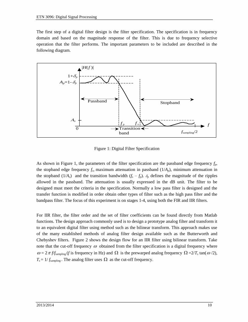
The first step of a digital filter design is the filter specification. The specification is in frequency

domain and based on the magnitude response of the filter. This is due to frequency selective

operation that the filter performs. The important parameters to be included are described in the

following diagram.

Figure 1: Digital Filter Specification

As shown in Figure 1, the parameters of the filter specification are the passband edge frequency fp,

the stopband edge frequency fs, maximum attenuation in passband (1/Ap), minimum attenuation in

the stopband (1/As) and the transition bandwidth (fs – fp). p defines the magnitude of the ripples

allowed in the passband. The attenuation is usually expressed in the dB unit. The filter to be

designed must meet the criteria in the specification. Normally a low pass filter is designed and the

transfer function is modified in order obtain other types of filter such as the high pass filter and the

bandpass filter. The focus of this experiment is on stages 1-4, using both the FIR and IIR filters.

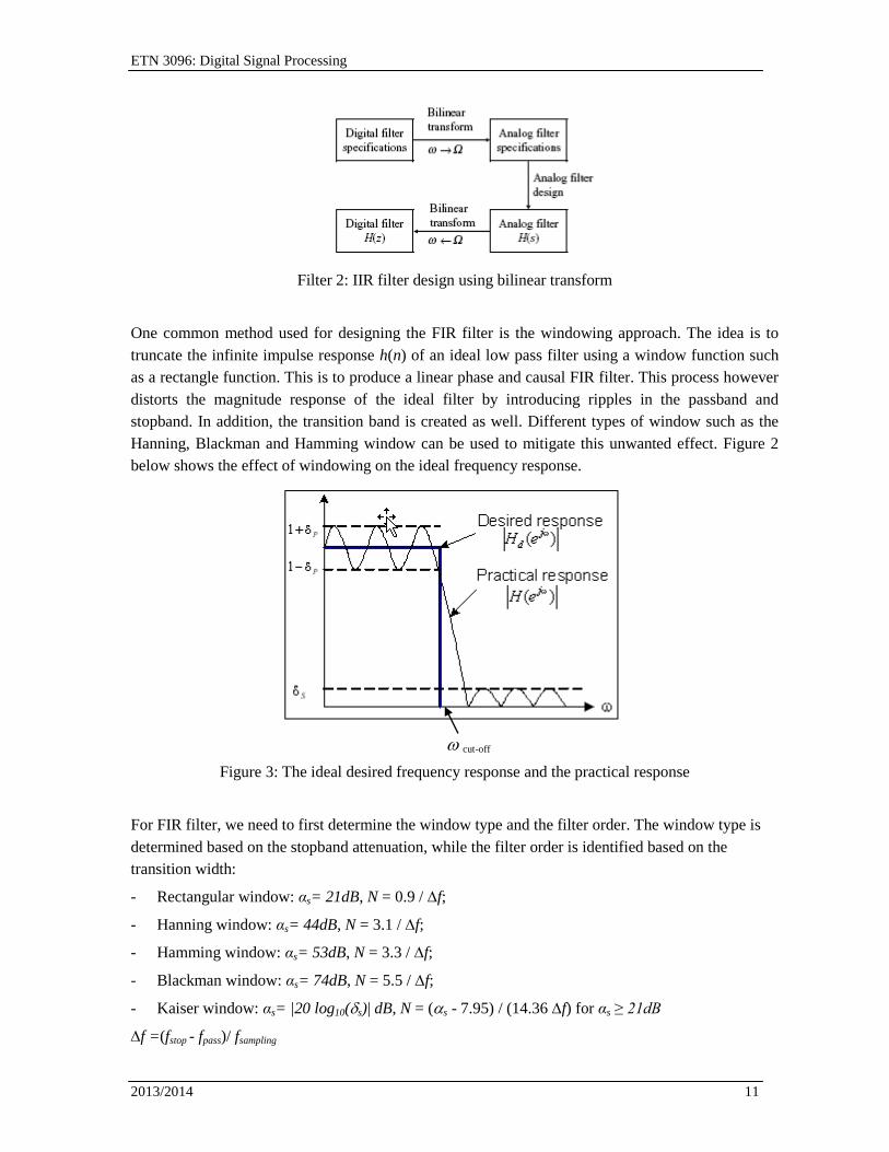
For IIR filter, the filter order and the set of filter coefficients can be found directly from Matlab

functions. The design approach commonly used is to design a prototype analog filter and transform it

to an equivalent digital filter using method such as the bilinear transform. This approach makes use

of the many established methods of analog filter design available such as the Butterworth and

Chebyshev filters. Figure 2 shows the design flow for an IIR filter using bilinear transform. Take

note that the cut-off frequency obtained from the filter specification is a digital frequency where

= 2 f/fsampling (f is frequency in Hz) and is the prewarped analog frequency =2/Ts tan( /2),

Ts = 1/ fsampling . The analog filter uses as the cut-off frequency.

|H( f )|

1+ p

Ap=1- p

s

0

Passband Stopband

Transition

band

f f p f s

fsampling/2


2013/2014 11

Filter 2: IIR filter design using bilinear transform

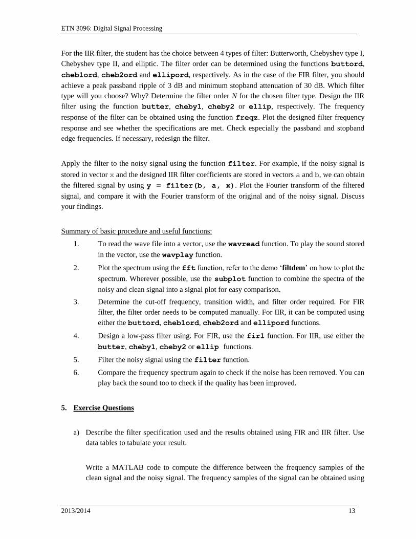
One common method used for designing the FIR filter is the windowing approach. The idea is to

truncate the infinite impulse response h(n) of an ideal low pass filter using a window function such

as a rectangle function. This is to produce a linear phase and causal FIR filter. This process however

distorts the magnitude response of the ideal filter by introducing ripples in the passband and

stopband. In addition, the transition band is created as well. Different types of window such as the

Hanning, Blackman and Hamming window can be used to mitigate this unwanted effect. Figure 2

below shows the effect of windowing on the ideal frequency response.

cut-off

Figure 3: The ideal desired frequency response and the practical response

For FIR filter, we need to first determine the window type and the filter order. The window type is

determined based on the stopband attenuation, while the filter order is identified based on the

transition width:

- Rectangular window: αs= 21dB, N = 0.9 / f;

- Hanning window: αs= 44dB, N = 3.1 / f;

- Hamming window: αs= 53dB, N = 3.3 / f;

- Blackman window: αs= 74dB, N = 5.5 / f;

- Kaiser window: αs= |20 log10(s)| dB, N = (s - 7.95) / (14.36 f) for αs ≥ 21dB

f =(fstop - fpass)/ fsampling


2013/2014 12

The filter coefficients of FIR filter can then be found using Matlab function.

4. Experimental Procedure

The audio signals need to be compared both in time and in frequency domain. To read the signal, use

the function wavread. You can also use the function wavread to identify the sampling frequency

of audio files (type ‘help wavread’). The length of the signal can be obtained using the

command length. The sound wave can be played using the command wavplay (don't be too

annoying for your fellow students by playing it over and over again…). Before the filter

specification can be obtained, the frequency spectrum of the clean and noisy signal will need to be

obtained. This enables you to locate the noise frequency range by comparing the spectrum plot for

both the clean and noisy signal. The frequency spectrum or Fourier transform can be obtained using

the command fft. Note that the fft is a complex function, hence it can be split up in its real and

imaginary parts (functions imag and real) or in its amplitude and phase (abs and angle).

Usually, we are more interested in the amplitude than in the phase - can you see why from the plot of

both phase and amplitude? You are only required to plot the spectrum magnitude until the Nyquist

frequency.

Plot the amplitude of the frequency spectrum for both the original clean signal and noisy signal.

From the comparison between both, specify the requirements for a filter that would eliminate the

noise as much as possible and alter the signal as little as possible. From passband edge frequency fp

and stopband edge frequency fs, the cutoff frequency fc is calculated as the average of both. The

student will have to implement both an FIR and an IIR filter. Although the concepts behind each

type of filter are very different, and their usage is also quite different, their design using MATLAB is

quite similar, thanks to the power of the MATLAB Signal Processing Toolbox.

For the FIR filter, the command fir1 will be used. For this experiment, you should achieve a peak

passband ripple of 3 dB and minimum stopband attenuation of 30 dB. Which window will you

choose? Why? Determine the filter order N for the chosen window. Design the FIR filter using the

function fir1. The frequency response of the filter can be obtained using the function freqz. Plot

the designed filter frequency response and see whether the specifications are met. Check especially

the passband and stopband edge frequencies. If necessary, redesign the filter.

Apply the filter to the noisy signal using the function filter. For example, if the noisy signal is

stored in vector x and the designed FIR filter coefficients are stored in vector h, we can obtain the

filtered signal by using y = filter(h, 1, x). Plot the frequency spectrum or Fourier

transform of the filtered signal, and compare it with the Fourier transform of the original and of the

noisy signal. Discuss your findings.


2013/2014 13

For the IIR filter, the student has the choice between 4 types of filter: Butterworth, Chebyshev type I,

Chebyshev type II, and elliptic. The filter order can be determined using the functions buttord,

cheb1ord, cheb2ord and ellipord, respectively. As in the case of the FIR filter, you should

achieve a peak passband ripple of 3 dB and minimum stopband attenuation of 30 dB. Which filter

type will you choose? Why? Determine the filter order N for the chosen filter type. Design the IIR

filter using the function butter, cheby1, cheby2 or ellip, respectively. The frequency

response of the filter can be obtained using the function freqz. Plot the designed filter frequency

response and see whether the specifications are met. Check especially the passband and stopband

edge frequencies. If necessary, redesign the filter.

Apply the filter to the noisy signal using the function filter. For example, if the noisy signal is

stored in vector x and the designed IIR filter coefficients are stored in vectors a and b, we can obtain

the filtered signal by using y = filter(b, a, x). Plot the Fourier transform of the filtered

signal, and compare it with the Fourier transform of the original and of the noisy signal. Discuss

your findings.

Summary of basic procedure and useful functions:

1. To read the wave file into a vector, use the wavread function. To play the sound stored

in the vector, use the wavplay function.

2. Plot the spectrum using the fft function, refer to the demo ‘filtdem’ on how to plot the

spectrum. Wherever possible, use the subplot function to combine the spectra of the

noisy and clean signal into a signal plot for easy comparison.

3. Determine the cut-off frequency, transition width, and filter order required. For FIR

filter, the filter order needs to be computed manually. For IIR, it can be computed using

either the buttord, cheb1ord, cheb2ord and ellipord functions.

4. Design a low-pass filter using. For FIR, use the fir1 function. For IIR, use either the

butter, cheby1, cheby2 or ellip functions.

5. Filter the noisy signal using the filter function.

6. Compare the frequency spectrum again to check if the noise has been removed. You can

play back the sound too to check if the quality has been improved.

5. Exercise Questions

a) Describe the filter specification used and the results obtained using FIR and IIR filter. Use

data tables to tabulate your result.

Write a MATLAB code to compute the difference between the frequency samples of the

clean signal and the noisy signal. The frequency samples of the signal can be obtained using


2013/2014 14

the MATLAB fft function. Use the code to estimate the noise frequency range. Your filter

design specifications depend on this estimation.

Noise frequency range (Hz): _____

Filter Specification

Sampling frequeny (Hz): ______ Nyquist Frequency (Hz) ____

Passband edge frequency (Hz): ____ Passband frequency range: ______

Stopband edge frequency (Hz): ______ Stopband frequency range: ______

Maximum passband attenuation (dB): _____ Minimum stopband attenuation (dB): ____

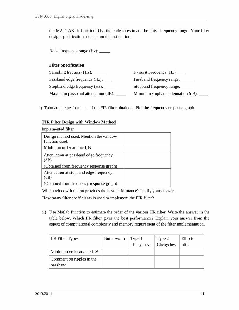
i) Tabulate the performance of the FIR filter obtained. Plot the frequency response graph.

FIR Filter Design with Window Method

Implemented filter

Design method used. Mention the window

function used.

Minimum order attained, N

Attenuation at passband edge frequency.

(dB)

(Obtained from frequency response graph)

Attenuation at stopband edge frequency.

(dB)


Which window function provides the best performance? Justify your answer.

How many filter coefficients is used to implement the FIR filter?

ii) Use Matlab function to estimate the order of the various IIR filter. Write the answer in the

table below. Which IIR filter gives the best performance? Explain your answer from the

aspect of computational complexity and memory requirement of the filter implementation.

IIR Filter Types Butterworth Type 1

Chebychev

Type 2

Chebychev

Elliptic

filter


Comment on ripples in the

passband


2013/2014 15

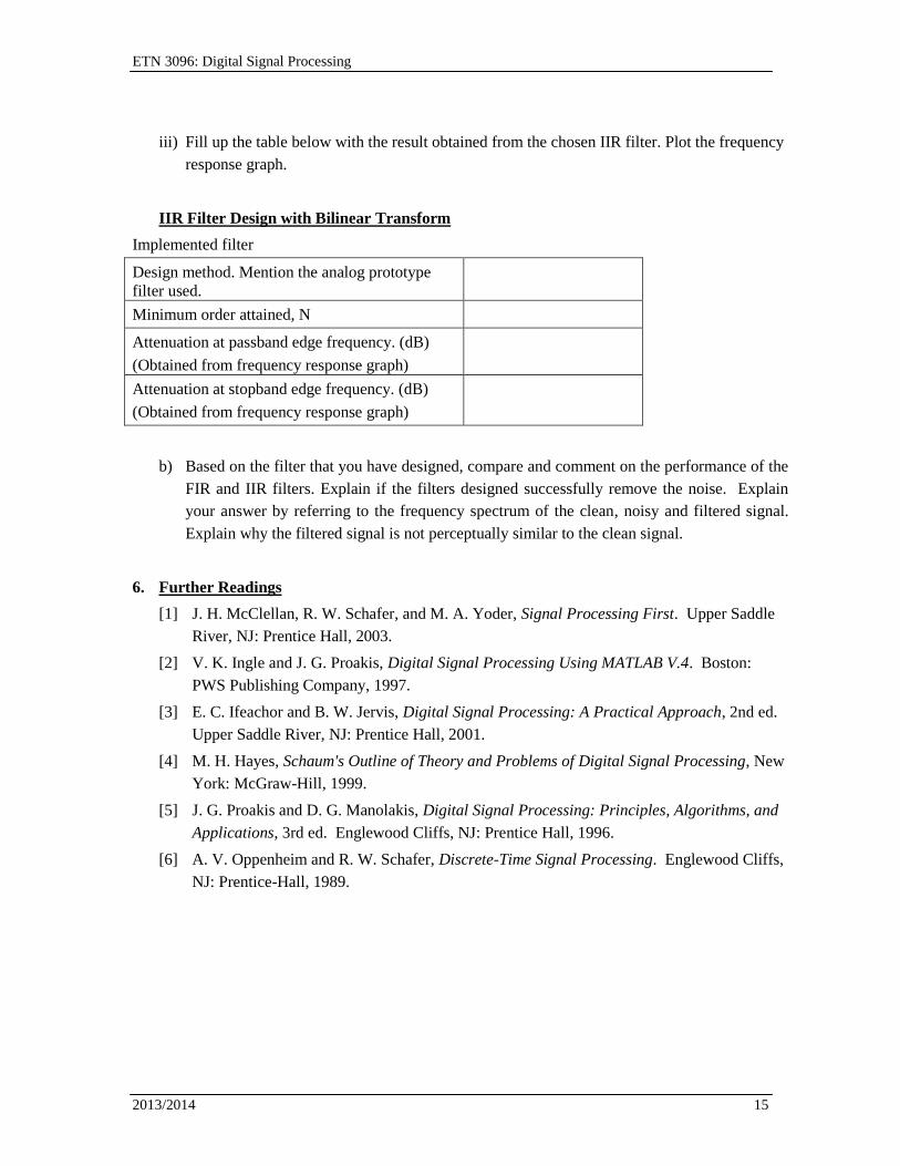
iii) Fill up the table below with the result obtained from the chosen IIR filter. Plot the frequency

response graph.

IIR Filter Design with Bilinear Transform

Implemented filter

Design method. Mention the analog prototype

filter used.


Attenuation at passband edge frequency. (dB)


Attenuation at stopband edge frequency. (dB)


b) Based on the filter that you have designed, compare and comment on the performance of the

FIR and IIR filters. Explain if the filters designed successfully remove the noise. Explain

your answer by referring to the frequency spectrum of the clean, noisy and filtered signal.

Explain why the filtered signal is not perceptually similar to the clean signal.

6. Further Readings

[1] J. H. McClellan, R. W. Schafer, and M. A. Yoder, Signal Processing First. Upper Saddle

River, NJ: Prentice Hall, 2003.

[2] V. K. Ingle and J. G. Proakis, Digital Signal Processing Using MATLAB V.4. Boston:

PWS Publishing Company, 1997.

[3] E. C. Ifeachor and B. W. Jervis, Digital Signal Processing: A Practical Approach, 2nd ed.

Upper Saddle River, NJ: Prentice Hall, 2001.

[4] M. H. Hayes, Schaum's Outline of Theory and Problems of Digital Signal Processing, New

York: McGraw-Hill, 1999.

[5] J. G. Proakis and D. G. Manolakis, Digital Signal Processing: Principles, Algorithms, and

Applications, 3rd ed. Englewood Cliffs, NJ: Prentice Hall, 1996.

[6] A. V. Oppenheim and R. W. Schafer, Discrete-Time Signal Processing. Englewood Cliffs,

NJ: Prentice-Hall, 1989.


2013/2014 16

7. Report Writing Guidelines

The lab report must be type written and shall consist of the following headings. Write clearly and

concisely to describe the important elements of your experiment. All graphs and tables need to be

labelled properly. Describe the data with proper units. The answer from the questions in section 5

can be incorporated into the result and discussion section. If there is any numerical calculation, it

needs to be shown in the procedure section. Do not forget to mention the filter specification and

design parameters used.

i) A header page

which mentions student name and ID number, subject, lab number, date of

experiment and date of report

ii) Introduction

This section introduces the basic theory underlying the experiment.

iii) Objectives

State the specific investigation that you would like to conduct in this

experiment.

iv) Procedures

Explain the procedure and the methodology used

v) Results and Discussion

Describe the results obtained in a suitable form such as table and graph.

Discuss the finding of the experiment from the result obtained.

vi) Conclusion

Derive conclusion based on your findings and results

vii) References

8. Report Submission Guidelines for DSP2

You are warned that any act of experiment data fabrication, copying of other people work and failure

to acknowledge the source of your information in the report (plagiarism) are serious offences and if

found, the student will be penalized. In addition to hard-copy submission, your soft-copy report

MUST also be submitted via email – allowing for "computer-aided copy detection" to be

executed.

WARNING: Students who are found to have copied someone else's report and the ones who

let somebody else copy their reports will all get their marks averaged. For example, two students

with similar reports originally deserving 20 marks each will each get 10 marks; and three students

with similar reports originally deserving 18 marks each will each get 6 marks instead. A complete

database of your seniors’ reports will also be used in the copy detection process. Plagiarizing

reports of previous years will result in getting zero marks.

Please read the following carefully, failing to comply with any item will result in mark reduction:

Please save your report in .doc format, .docx format will not be accepted.

In case the file size of the report exceeds 2Mbyte, it should be compressed using

ZIP/RAR. The filename of the report/zipped report should be your student ID number (e.g.

the lab report of student with ID number 95100107 should be "95100107.doc").


2013/2014 17

Students also need to submit two .wav files: one for the noisy signal filtered using the

designed FIR filter, and the other for the noisy signal filtered using the designed IIR filter.

The filename of the .wav files should be the student ID number followed by the letter i or

f, corresponding to the IIR or the FIR filter (e.g. the sound file of the signal filtered with

the IIR filter of student with ID number 95100107 should have the name

"95100107i.wav").

Attach and email the THREE FILES mentioned above to [email protected]. Emails

sent to the lecturer’s email address will not be considered. In your email’s subject heading,

please simply write ‘Re: DSP2 Lab Report Submission’.

mailto:[email protected]


2013/2014 18

Demo on the DSP Starter Kit

In DSP2, a demonstration on the use of the DSP starter kit (DSK) for Texas Instrument’s

TMS320C55xx processor will be given. In the following, some background information on real-time

DSP implementation using general-purpose DSP processors is given.

Overview

The demonstration setup for the real-time DSP implementation consists of

Texas Instrument’s DSP Starter Kit, TMS320VC5510

Headphone or Speaker

Multimedia PC

Code Composer Studio

o A DSP development tool that allows users to create, edit, build, debug and

analyse DSP programs either in a simulated environment or actual real-time

implementation into the DSP processor.

Matlab

o Design of DSP programs such as FIR and IIR filters using common

programming language such a C.

The objective of the setup is to demonstrate the work flow of designing a FIR filter using Matlab

(such as FDATool) and to implementation the designed filter onto a real-time DSP processor.

During the demonstration you will see that signals are being fed into the DSP board continuously

and output will be generated at real-time. This is possible with the DSP processor working multiple

times faster that the incoming signal to process and execute according to the loaded program (For

this demonstration we have loaded in a simple FIR LPF filter).

The work flow begins by designing a FIR filter using Matlab that meets certain requirements such

as;

the type of filters; LPF (Low Pass Filter), BPF (Band pass Filter)

no. of coefficients

Block Diagram of TMS320VC5510 DSK

Board

Audio signal

from PC’s audio

out

Headphone


2013/2014 19

cut-off frequency preferred filter

After the FIR filter has been designed, the filter is simulated under Matlab to obtain information

such as its frequency response and stability. This is to ensure that the designed filter meets the stated

requirements. Any changes or adjustment may be performed at this stage. After the filter is designed,

it will result in a few parameters i.e. the number of filter coefficients, value for each filter coefficient

and sampling period. These parameters will be loaded into the DSK board together with a program

written in CCS. This program will process the incoming signal with the obtained parameters. For

this demonstration, an FIR filter algorithm program is chosen and is written in C language using

CCS (Code Composer Studio). The FIR filter algorithm program will utilise the parameters

obtained.

The DSK board works under the CCS and communicates with it through its onboard USB (Universal

Serial Bus) JTAG Emulator as shown in the figure above. Therefore the FIR filter algorithm

program will perform the following task onto the DSK board (refer to signal flow graph shown

below):

Initiate all the necessary configuration such as sampling period, codec configuration,

memory allocation and etc.

Fetch the signal stored in the memory

Perform convolution between the stored signal and the coefficient values obtained

earlier using Matlab

Stored the resultant value

Signal Flow Graph

The resultant values will then be converted to an output signal via the DAC codec. The output signal

will contain the filtered input signal. In other words, the output signal is actually a convolution result

between the coefficients and the input signal. During the demonstration, a noisy signal will be the

Audio signal from

PC’s audio output

ADC Codec

Input signal is stored

in Memory (SDRAM)

DSP Processor (Convolution of the input signal and the filter coefficients)

Loaded FIR Filter Program

via Code Composer Studio

Headphone

DAC Codec

Resultant is stored in

Memory (SDRAM)

Filter coefficients


2013/2014 20

input signal and the DSK board will be programmed to be a FIR filter. The output of the DSK board

will be a clean signal with the noise removed.

Throughout the demonstration you will witness the workflow of implementing the theoretical DSP

knowledge to a realisable real-time DSP application.

Appendix

Software tools are computer programs that have been written to perform specific operations. Most

DSP operations can be categorized as being either analysis tasks or filtering tasks. Signal analysis

deals with the measurement of signal properties. MATLAB is a powerful environment for signal

analysis and visualization, which are critical components in understanding and developing a DSP

system. C programming is an efficient tool for performing signal processing and is portable over

different DSP platforms.

MATLAB is an interactive, technical computing environment for scientific and engineering

numerical analysis, computation, and visualization. Its strength lies in the fact that complex

numerical problems can be solved easily in a fraction of the time required with a programming

language such as C. By using its relatively simple programming capability, MATLAB can be easily

extended to create new functions, and is further enhanced by numerous toolboxes such as the Signal

Processing Toolbox and Filter Design Toolbox. In addition, MATLAB provides many graphical user

interface (GUI) tools such as Filter Design and Analysis Tool (FDATool).

The purpose of a programming language is to solve a problem involving the manipulation of

information. The purpose of a DSP program is to manipulate signals to solve a specific signal

processing problem. High-level languages such as C and C++ are computer languages that have

English-like commands and instructions. High-level language programs are usually portable, so they

can be recompiled and run on many different computers. Although C/C++is categorized as a high-

level language, it can also be written for low-level device drivers. In addition, a C compiler is

available for most modern DSP processors such as the TMS320C55x. Thus C programming is the

most commonly used high-level language for DSP applications.

C has become the language of choice for many DSP software development engineers not only

because it has powerful commands and data structures but also because it can easily be ported on

different DSP processors and platforms. The processes of compilation, linking/loading, and

execution are outlined in Figure 1.

Figure 1. Program compilation, linking, and execution flow


2013/2014 21

C compilers are available for a wide range of computers and DSP processors, thus making the C

program the most portable software for DSP applications. Many C programming environments

include GUI debugger programs, which are useful in identifying errors in a source program.

Debugger programs allow us to see values stored in variables at different points in a program, and to

step through the program line by line.

The manufacturers of DSP processors typically provide a set of software tools for the user to

develop efficient DSP software. The basic software development tools include C compiler,

assembler, linker, and simulator. In order to execute the designed DSP tasks on the target system, the

C or assembly programs must be translated into machine code and then linked together to form an

executable code. This code conversion process is carried out using software development tools

illustrated in Figure 2.

Figure 2. TMS320C55x software development flow and tools


2013/2014 22

The TMS320C55x software development tools include a compiler, an assembler, a linker, an

archiver, a hex conversion utility, a cross-reference utility, and an absolute lister. The C55x C

compiler generates assembly source code from the C source files. The assembler translates assembly

source files, either hand-coded by DSP programmers or generated by the C compiler, into machine

language object files. The assembly tools use the common object file format (COFF) to facilitate

modular programming. Using COFF allows the programmer to define the system’s memory map at

link time. This maximizes performance by enabling the programmer to link the code and data objects

into specific memory locations. The archiver allows users to collect a group of files into a single

archived file. The linker combines object files and libraries into a single executable COFF object

module. The hex conversion utility converts a COFF object file into a format that can be

downloaded to an EPROM programmer or a flash memory program utility.

The DSK is a low-cost development board for the user to develop and evaluate DSP algorithms

under a Windows operation system environment. In this demo, we will use the Spectrum Digital’s

TMS320VC5510 DSK for real-time experiments. The DSKworks under the Code Composer Studio

(CCS) development environment. The DSK package includes a special version of the CCS. The

DSK communicates with CCS via its onboard universal serial bus (USB) JTAG emulator. The

C5510 DSK uses a 200 MHz TMS320VC5510 DSP processor, an AIC23 stereo CODEC, 8 Mbytes

synchronous DRAM, and 512 Kbytes flash memory.

Texas Instruments’ CCS Integrated Development Environment (IDE) is a DSP development tool

that allows users to create, edit, build, debug, and analyze DSP programs. For building applications,

the CCS provides a project manager to handle the programming project. For debugging purposes, it

provides breakpoints, variable watch windows, memory/register/stack viewing windows, probe

points to stream data to and from the target, graphical analysis, execution profile, and the capability

to display mixed disassembled and C instructions. Another important feature of the CCS is its ability

to create and manage large projects from a GUI environment. In this demo, we will use simple

examples to show you the basic editing features, key IDE components, and the use of the C55x DSP

development tools.

Procedures of the demo are listed as follows:

1. Create a project for the CCS: Choose Project→New to create a new project file and save it.

The CCS uses the project to operate its built-in utilities to create a full-build application.

2. Create C program files using the CCS editor: Choose File→New to create a new file, type in

the C code and save it as a C source file. 3. Create a linker command file for the simulator: The command file (with extension .cmd) is used

by the linker to map different program segments into a prepartitioned system memory space. 4. Setting up the project: Add the C and cmd files to the project by choosing Project→Add

Files to Project. Programs written in C language require the use of the run-time support

library, either rts55.lib or rts55x.lib, for system initialization. This can be done by

selecting the compiler and linker dialog box and entering the C55x run-time support library,

rts55.lib, and adding the header file path related to the source file directory.


2013/2014 23

5. Build and run the program: Use Project→Rebuild All command to build the project. If

there are no errors, the CCS will generate the executable output file (extension .out). Before

we can run the program, we need to load the executable output file to the C55x DSK or the

simulator. To do so, use File→Load Program menu and select the .out file and load it.

Execute this program by choosing Debug→Run. The processor status at the bottom-left-hand

corner of the CCS will change from CPU HALTED to CPU RUNNING. The running process

can be stopped by the Debug→Halt command. We can continue the program by reissuing the

Run command or exiting the DSK or the simulator by choosing File→Exit menu.

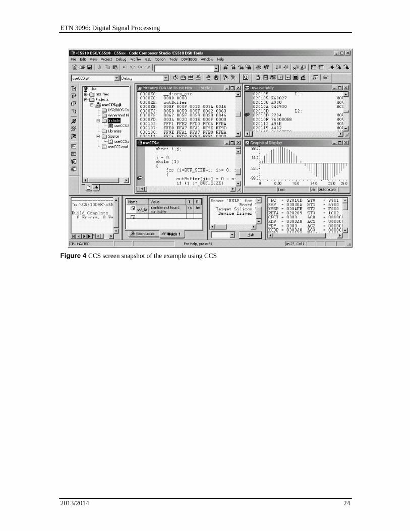
The photo of the C5510 DSK is shown in Figure 3. A CCS screen snapshot is shown in Figure 4.

Figure 3. TMSVC 5510 DSK


2013/2014 24

Figure 4 CCS screen snapshot of the example using CCS


2013/2014 25

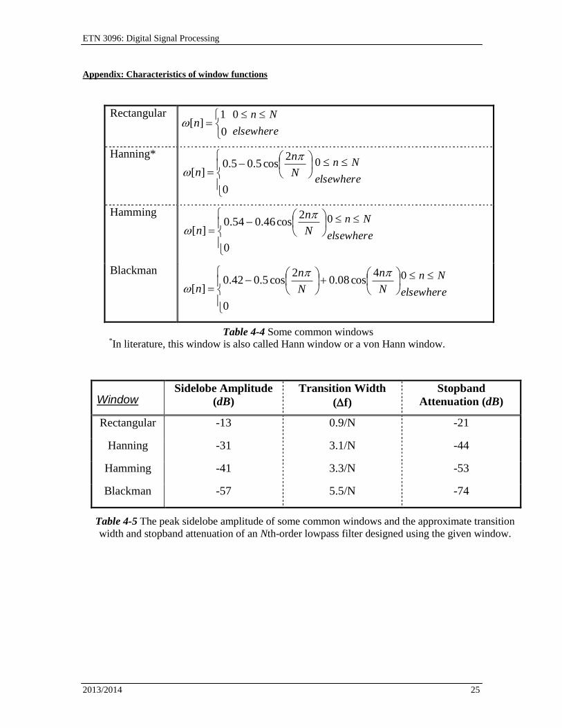
Appendix: Characteristics of window functions

Rectangular

0

1][n

elsewhere

Nn 0

Hanning*

0

2cos5.05.0

][ N

n

n

elsewhere

Nn 0

Hamming

0

2cos46.054.0

][ N

n

n

elsewhere

Nn 0

Blackman

0

4cos08.0

2cos5.042.0

][ N

n

N

n

n

elsewhere

Nn 0

Window Sidelobe Amplitude

(dB)

Transition Width

(f)

Stopband

Attenuation (dB)

Rectangular -13 0.9/N -21

Hanning -31 3.1/N -44

Hamming -41 3.3/N -53

Blackman -57 5.5/N -74

Table 4-4 Some common windows *In literature, this window is also called Hann window or a von Hann window.

Table 4-5 The peak sidelobe amplitude of some common windows and the approximate transition

width and stopband attenuation of an Nth-order lowpass filter designed using the given window.

FACULTY OF ENGINEERING MULTIMEDIA UNIVERSITYfoe.mmu.edu.my/lab/lab sheet/LABSHEET TRIM2...

Documents

Transcript of FACULTY OF ENGINEERING MULTIMEDIA UNIVERSITYfoe.mmu.edu.my/lab/lab sheet/LABSHEET TRIM2...