Dynamic load factors with damping

Item Type text; Thesis-Reproduction (electronic)

Authors Toriello, Michael Raymond, 1947-

Publisher The University of Arizona.

Rights Copyright © is held by the author. Digital access to this materialis made possible by the University Libraries, University of Arizona.Further transmission, reproduction or presentation (such aspublic display or performance) of protected items is prohibitedexcept with permission of the author.

Download date 29/06/2018 20:25:05

Link to Item http://hdl.handle.net/10150/347984

DYNAMIC.LOAD FACTORS WITH DAMPING

by

Michael Raymond Toriello

A Thesis Submitted to the Faculty of the

DEPARTMENT OF CIVIL ENGINEERING AND ENGINEERING MECHANICS

In Partial Fulfillment of the Requirements For the Degree of

MASTER OF SCIENCE WITH A MAJOR IN CIVIL ENGINEERING

In the Graduate College

THE UNIVERSITY OF ARIZONA

1 9 7 6

STATEMENT BY AUTHOR

This thesis has been submitted in partial fulfillment of re­quirements for an advanced degree at The University of Arizona and is deposited in the University Library to be made available to borrowers under rules of the Library.

Brief quotations from this thesis are allowable without special permission, provided that accurate acknowledgment of source is made* Requests for permission for extended quotation from or reproduction of this manuscript in whole or in part may be granted by the head of the major department or the Dean of the Graduate College when in his judg­ment the proposed use of the material is in the interests of scholar­ship, In all other instances, however, permission must be obtained from the author.

APPROVAL BY THESIS DIRECTOR

This thesis has been approved on the date shown below:

RALPH M.' RICHARD Professor of Civil Engineering and

Engineering Mechanics

ACKNOWLEDGMENTS

I wish to express my gratitude to Professor Ralph M, Richard for

his assistance and guidance in the development of this thesis project

and throughout my graduate studies.

Very special thanks to my wife, Jane, for her patience and

encouragement,

TABLE OF CONTENTS

Page

LIST OF I L L U S T R A T I O N S ........................ . v

ABSTRACT . . . . . ........... vii

CHAPTER

1. INTRODUCTION . 1

Definitions . . . . . . . . . . . . . . . . . . . . . 1Dynamic Load F a c t o r ........... 2Viscous Damping .................... . . . . . . . 3Coulomb Damping ......... . . . . . . . . . . . . 4Structural Damping . . . . . . . . . . . . . . . . 5

2. MOTION EQUATIONS FOR VISCOUS, COULOMB AND STRUCTURALDAMPING . . . . . . . . . . . . . . . . . 6

Motion Equations for Viscous Damping . . . . . . . . . 6Motion Equations for Coulomb Damping . . . . . . . . . 10Motion Equations for Structural Damping . . . . . . . 12Numerical Integration Method Application to

the Motion Equations . . . . . . . . . . . . . . . 15

3. COMPUTER PROGRAM DEVELOPMENT .............. . . . . . . . . 22

Program LODFACT . . . . . . . . . . . . . . 22Program Features ................ . . . . . . . . . 22

4. PRESENTATION OF RESULTS . . . . . . . . . . . . . . . . . 25

Rectangular Pulse Load . . . . . . . . . . . 25Data Check . . . . . . . . . . . . . . . . . . . . . . 29Triangular Pulse Load . . . . . . . . . . . . . . . . 34Ramp Load ........... 35

5. SUMMARY AND CONCLUSIONS . . . . . .............. . . . . . 44

APPENDIX A: NOTATION . . . . . . . . . . . . . . . . . . . . . . . 45

REFERENCES . . . . . . . . . . . . . . . . . . . . . . . . . . . . 47

iv

LIST OF ILLUSTRATIONS

Figure • Page

1. System with viscous damping . . . . . . . . . . . . . . . 3

2. System with Coulomb damping . . . . . . . . . . 4

3. Free body diagram for viscous d a m p i n g .................. . „ 6

4. Free body diagram for Coulomb damping ........... 10

5. Free body diagram for structural damping . . . . . . . . . 12

6. Random load varying with time . .............. 16

7. Linear variation of acceleration . . . . . . . . . . . . . 16

8. Approximated loading function for a blast load . . . . . . 23

9. Rectangular pulse load . . . . . . . . . . . . . . . . . . 25

10. Dynamic load factor for rectangular pulse load withviscous damping . . . . . . . . . . . . .......... . . . . 26

11. Dynamic load factor for rectangular pulse load withCoulomb damping . . . . . . . . . . . . . . . . . . . . . 27

12. Dynamic load factor for rectangular pulse load withstructural damping . . . . . . . . . . . . . . . . . . . . 28

13. Triangular pulse load . . . . . . . . . . . . . . . . . . 34

14. Dynamic load factor for triangular pulse load withviscous damping . . . . . . . . . . . . . . . . . . . . . 36

15. Dynamic load factor for triangular pulse load withCoulomb damping . . . . . . . . . . . . . . . . . . . . . 37

16. Dynamic load factor for triangular pulse load withstructural damping . . . . . . . . . . . . . . . . . . . . 38

17. Ramp load . ............ . . . . . . . . . . . . . . . . . 39

v

viLIST OF ILLUSTRATIONS”"Continued

Figure Page

18, Dynamic load factor for ramp load with viscous damping , . 40

19c Dynamic load factor for ramp load with Coulomb damping . 0 41

20, Dynamic load factor for ramp load with structural damping, 42

ABSTRACT

For various loading functions dynamic response curves are de­

veloped for three types of damping, viscous. Coulomb and structural.

It is shown that damping may have a very definite effect on the amount

of dynamic response even for short, impulse type loadings.

Equations of motion are derived for the three damping types and

a computer program devised for the solution by numerical integration.

By varying the damping coefficients with each loading function, dynamic

load factor charts are developed for viscous. Coulomb and structural

damping.

Although a great deal of work has been done in the area of

dynamic load factors for the undamped case less consideration has been

given for effects of damping in the case of impulse loadings.

CHAPTER 1

INTRODUCTION

Dynamic loads are of more concern today to the structural design

engineer than ever before with increased emphasis on earthquake designs

and the continuing concern for wind and blast loadings.

The concept of the dynamic load factor is used to correlate the

static and dynamic load effects on a structure. In developing dynamic

load factor charts, consideration must be given to the magnitude and

duration of the applied load, along with the stiffness, natural period

and damping coefficient and type of damping for the structure.

Extensive work has been done in the development of dynamic load

factor charts for the undamped case (Biggs et al. 1959). For most

engineering purposes the response for undamped vibration is considered

an adequate approximation for the actual damped condition (Biggs et al.

1959). The effects of damping however are very important in relation to

dynamic response. In some instances when damping is large enough, the

dynamic effect can be less than the static.

Definitions

The definition and a detailed explanation of the significance of

dynamic load factors and the three types of damping (viscous. Coulomb

and structural) follow.

1

Dynamic Load Factor

The dynamic load factor is a non-dimensional factor by which the

static displacement (Xg) produced by a reference load P applied as a

static load should be multiplied by in order to obtain the dynamic

displacement (^ ) if P is a function of time. It is simply the ratio

of dynamic displacement to static displacement, i.e..

Df - J (1)

The static displacement X g can be represented as

Xs ■ f <2>

where Pq is the reference applied static load and k the stiffness.

Using the expression for X g Equation 1 becomes

kXDf = (3).

o

After calculation of the maximum values of dynamic displacement

for a given loading function are made, dynamic load factors are then

determined (Equation 3) and plotted against the non-dimensional factor

t /T where t is a reference duration of the applied load and T the o onatural period of the structure.

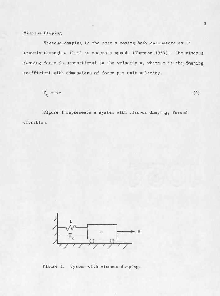
Viscous Damping

Viscous damping is the type a moving body encounters as it

travels through a fluid at moderate speeds (Thomson 1953). The viscous

damping force is proportional to the velocity v, where c is the damping

coefficient with dimensions of force per unit velocity.

Figure 1 represents a system with viscous damping, forced

vibration.

Fv cv (4)

/ k

Pm

Figure 1. System with viscous damping.

4

Coulomb Damping

Coulomb damping, or dry damping, results from the friction

forces during sliding between dry surfaces (Thomson 1953). The force

is opposite to the velocity, but constant,

Fc = p,N (5)

where ^ is the coefficient of friction and N the normal force. Figure 2

represents a system with Coulomb damping.

/zm

I n

Figure 2. System with Coulomb damping,

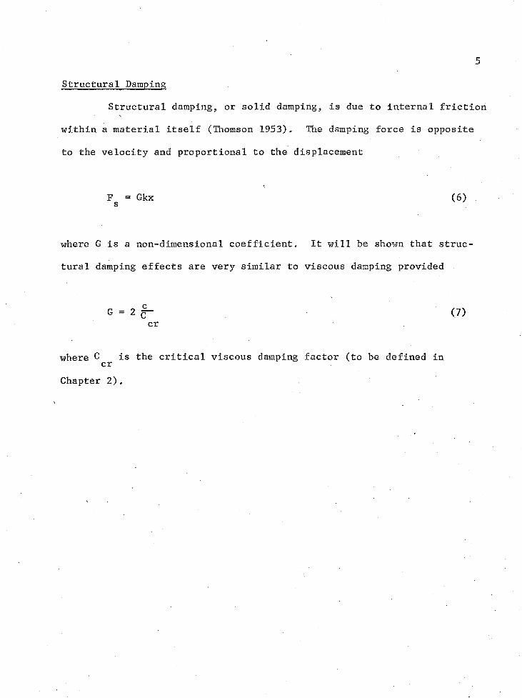
Structural Damping

Structural damping, or solid damping, is due to internal friction

within a material itself (Thomson 1953), The damping force is opposite

to the velocity and proportional to the displacement

Fg = Gkx (6)

where G is a non-dimensional coefficient. It will be shown that struc­

tural damping effects are very similar to viscous damping provided

G = 2 q (7)cr 1

where is the critical viscous damping factor (to be defined in

Chapter 2).

CHAPTER 2

MOTION EQUATIONS FOR VISCOUS, COULOMB AND STRUCTURAL DAMPING

In developing dynamic load factor charts motion equation for

each condition of damping are required to calculate acceleration,

velocity and displacement for the various loading conditions.

Motion Equations for Viscous Damping

Figure 3 represents a free body diagram for the system in Figure

1 viscous damping with forced vibration with x representing the displace-2 2ment; x = dx/dt the velocity; and x = d x/dt the acceleration.

mx ^ k x _ mg

t

f m g

Figure 3. Free body diagram for viscous damping.

Summing the forces in the horizontal direction the equation of motion

for Figure 3 becomes

mx + cx + kx = P (8)

where mx is the inertia force, cx the damping force, and kx the spring

force. Dividing Equation 8 by the mass m gives

x + ^x -f- Mx = ~ (9)m m m

The undamped circular frequency tu can be expressed as (Hinkle, Morse

and Tse 1963)

2 kw = - (10)m

Substituting Equation 10 into Equation 9 gives

x + Mfe + (JU x = — (11)m m

Equation 11 represents the equation of motion for a system with viscous

damping and forced vibration.

Now consider the same system with viscous damping but in free

vibration. The equation of motion for the system in Figure 1 without

P becomes

8

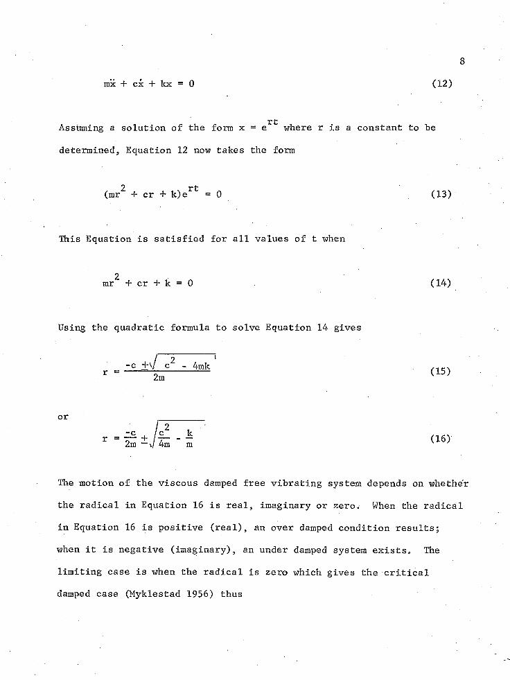
mx + cx + kx = 0 (12)

rtAssuming a solution of the form x = e where r is a constant to be

determined. Equation 12 now takes the form

(mr2 + cr + k)ert = 0 (13)

This Equation is satisfied for all values of t when

2mr -f cr *f k = 0 (14)

Using the quadratic formula to solve Equation 14 gives

r - -c c2 - 4mk (15)zm

or

<16>

The motion of the viscous damped free vibrating system depends on whether

the radical in Equation 16 is real, imaginary or zero. When the radical

in Equation 16 is positive (real), an over damped condition results;

when it is negative (imaginary), an under damped system exists. The

limiting case is when the radical is zero which gives the critical

damped case (Myklestad 1956) thus

9

f H <» >4m

Solving for critical damping

C _ = 2 x/(k/m)m2 (18)cr

Using the expression for circular frequency from Equation 10, critical

damping can be expressed as

/ 2 2'Ccr = 2 \/w m = 2(Dm (19)

Equation 11 may be written as

5 + C- x + co2x = (20)cr

Viscous damping can now be expressed as a percent of critical damping

where

Y = •§— (21)cr

Substituting the expressions for critical damping Equation 19 and 21

into Equation 20 gives

2 px + 2u)Yx 110 x = ^ (22)

10Equation 22 is the equation of motion for viscous damping with forced

vibration with damping represented as a percent of critical damping.

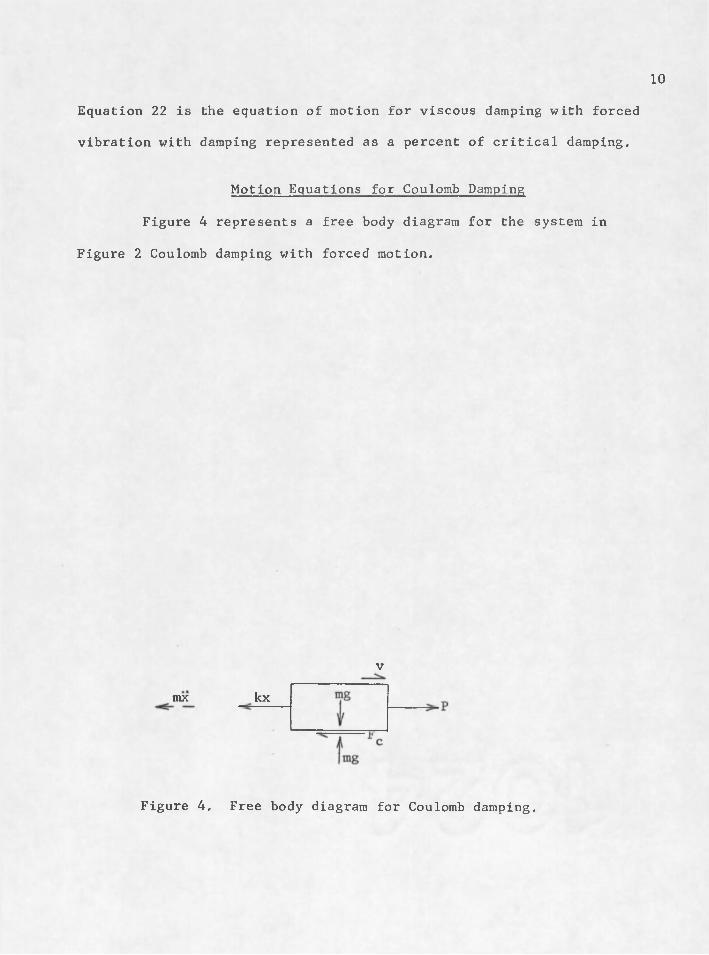
Motion Equations for Coulomb Damping

Figure 4 represents a free body diagram for the system in

Figure 2 Coulomb damping with forced motion.

v

mx kx

Figure 4. Free body diagram for Coulomb damping.

11Summing the forces in the horizontal direction the equation of motion

for Figure 4 becomes

mx 4- Fc + kx = P (23)

Dividing through by the mass m gives

*c k Px 4- — - -i— x = — (24)m m m

Again using the expression for circular frequence Equation 24 reduces

to

*C 2 Px 4 h cu x = (25)m m

The term F^ represents the frictional resistance or Coulomb damping as

defined previously in Chapter 1. Coulomb damping is constant (a function

of the material at contact surface) but always opposite to the velocity.

Therefore Equation 5 may be written

Fc = ^ Dc (26)

where

N = mg (27)

and

D = c

12The term allows the frictional force to act opposite the velocity.

The Coulomb damping force can now be expressed as

Fc = p-mgDc (29)

Substituting Equation 29 into Equation 25 gives

x + pgD + cu^x = — (30)c m

Equation 30 is the equation of motion for Coulomb damping with forced

motion.

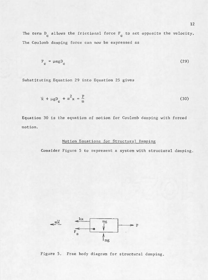
Motion Equations for Structural Damping

Consider Figure 5 to represent a system with structural damping,

_^kx mgV

rax

p * 1s f1 mg

Figure 5. Free body diagram for structural damping.

13

Summing the forces in the horizontal direction the equation of motion

for Figure 5 becomes

mx + Fg + kx = P (31)

Dividing through by the mass and introducing the circular frequency a)

Equation 31 reduces to

Fo ? Px + — — h a) x = (32)m m

The term Fg represents the structural damping force resulting from

internal friction within the material defined by Equation 6» This

damping force is proportional to the displacement but opposite to the

velocity therefore Equation 6 becomes

Fg = Gkx Dg (33)

where

D = sx

LW- = ± 1 (34)

The term Dg allows the damping force to act opposite the velocity. The

structural damping force can now be represented as

Fg = GkxDg (35)

14

Substituting the above expression into Equation 32 gives

GkxDs 2 Px H-------- h 0) x = — (36)m m

Using the expression for circular frequency

2 2 Px + a ) G D x + U)x = ‘” (37)s m

or

x + 0)2x [GD + 1] = - (38)s m

Equation 38 represents the equation of motion for structural damping

with forced vibration.

In Equation 37 let the structural damping coefficient G equal

to twice the percent critical damping (Y)

G = 2“ = 2Y (39)cr

Substituting the expressions represented by Equations 34 and 39 into

Equation 37

x + U)22Y

or

15

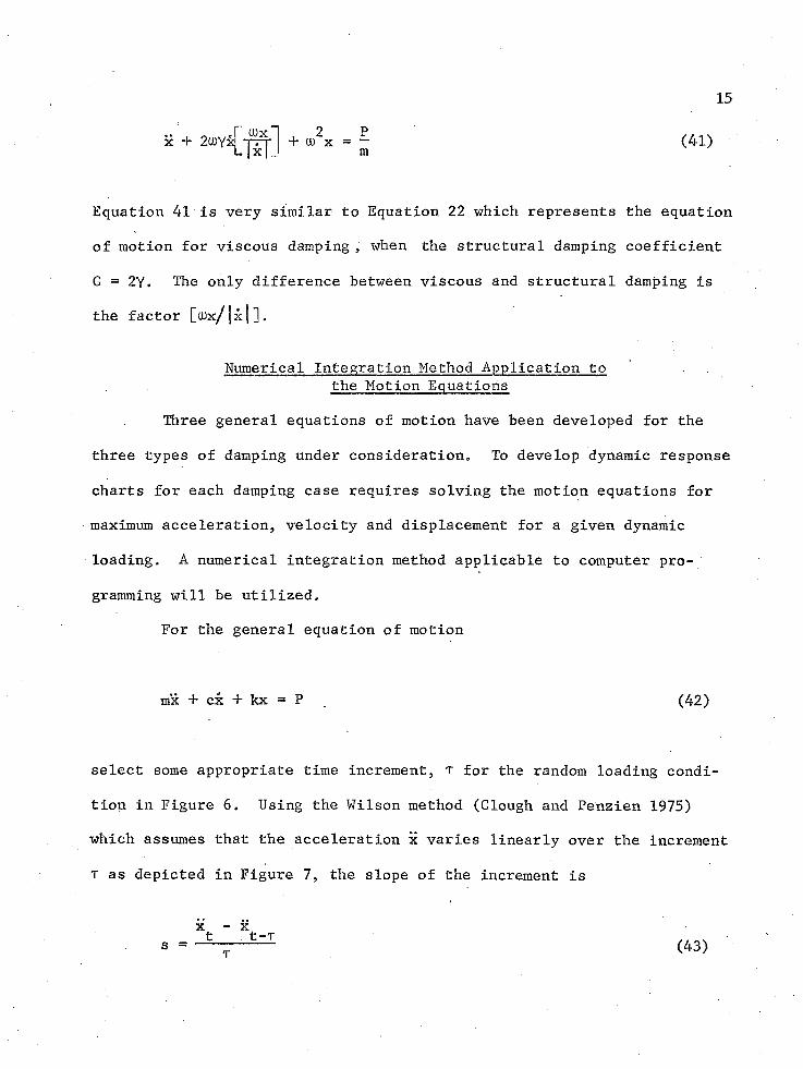
x + 2udyx ' (Ox.Hi- + uo^x = — (41)m

Equation 41 is very similar to Equation 22 which represents the equation

of motion for viscous damping , when the structural damping coefficient

G = 2Y« The only difference between viscous and structural damping is

the factor [a)x/|x| ],

Numerical Integration Method Application to the Motion Equations

Three general equations of motion have been developed for the

three types of damping under consideration. To develop dynamic response

charts for each damping case requires solving the motion equations for

maximum acceleration, velocity and displacement for a given dynamic

loading. A numerical integration method applicable to computer pro­

gramming will be utilized.

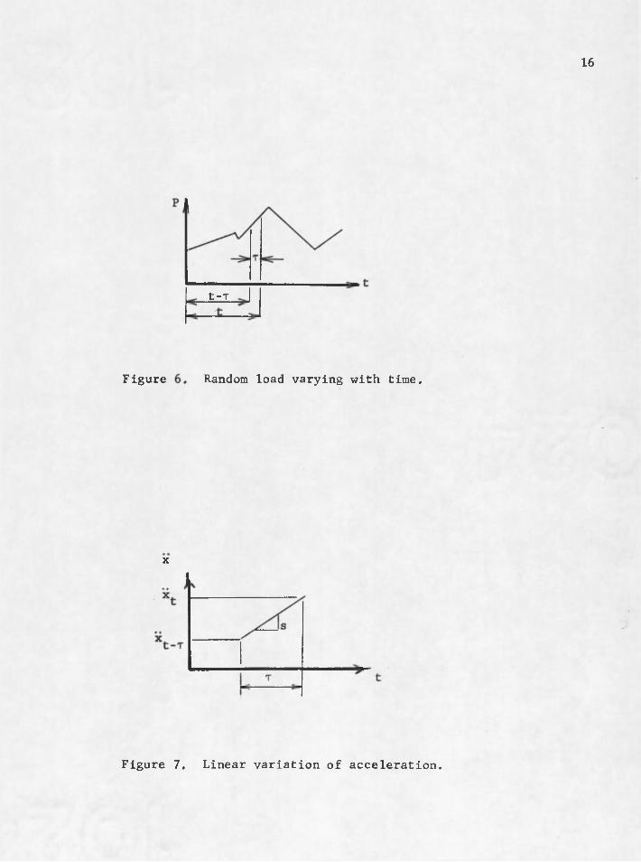
For the general equation of motion

mx + cx -f kx = P , (42)

select some appropriate time increment, t for the random loading condi­

tion in Figure 6. Using the Wilson method (Clough and Penzien 1975)

which assumes that the acceleration x varies linearly over the increment

r as depicted in Figure 7, the slope of the increment is

x. - x_8 = - 1 (43)

16

Figure

x

t-T

Random load varying with time.

Figure 7. Linear variation of acceleration.

17

or

*t = *t-T + ST (44)

Integrating equation 44 from zero to t to get the velocity

xt =ST

xtdT = Xt-TT + \ - r 2 (45)

Integrating again to get the displacement

xt %X |--t T ST'

V T = ^ 2 — + ^t-T7 + X t-T + T (46)

Now substituting the expression for s (Equation 43) into Equations

45 and 46

Xt = X t-TT + Xt-T + K ' T t'T] (47)

or

(48)

and

X T n * *T + +

t-T t-T 6 L T (49)

or

18

X T2 X T 2x t = ™ i + i t-TT + X t-T + 1 (50)

For programming purposes in Equation 48 let

Xt -t Ta = " Y " + xt.T (51)

and in Equation 50 let

.2

B “ + Xt—TT + Xt-T (52)

The equation for velocity now becomes

X tTxt = -y- + A (53)

and for the displacement

v 2xt - - f - + B (54)

The expressions developed for velocity and displacement are in

terms of acceleration and variables A and B which can be easily calcu­

lated. Using these expressions the three equations of motion developed

earlier in this chapter can be solved in terms of acceleration.

First consider Equation 22 the expression for viscous damping,

substituting the expressions for velocity (Equation 53) and displacement

(Equation 54) gives

19

x + + a J + + b] = £ (55)

separation of terms gives

x(l + cuyr + o) t ^/6) = P/m - 2u)yA - cu2B (56)

Now define

b = (1 + OUYT + u)2t 2/6) (57)

The final expression for acceleration for viscous damping becomes

x = ^ YA ' (58)V

Substituting the expression for displacement (Equation 54) into

30 which defines motion for Coulomb damping gives

2x + p,gD^ + ct2[^l 1- BJ = ^ (59)

separating terms

2 2 2 x(l + w r /6) = P/m - ngD^ - a) B (60)

Now define

b = (1 + cu^ t ^/6) (61)

The final expression for acceleration associated with Coulomb damping

x =P/m - p,gD - U) B c (62)

Using the expression for displacement (Equation 54) in Equation

38 which defines motion with structural damping gives

x + <D |_GDs + 1 xt£ _ 6 + B = P/m (63)

separating terms

2 2 2 2 2 2 x(l + (JO t GDg/6 + (JO r /6) = P/m - uo GD^B - (JO B (64)

and define

b ® (1 + (J02 T 2 G D g /6 + (J02 t 2 /6) (65)

The final expression for acceleration for structural damping becomes

2 1

Equations 589 62 and 66 along with the expressions for

bg9 A and B allow for calculations of acceleration for each damping

condition for the various loading conditions. Equations 53 and 54 allow

for calculations of velocity and displacement respectively in terms of

acceleration.

CHAPTER 3

COMPUTER PROGRAM DEVELOPMENT

The equations of motion developed in Chapter 2 for each condi­

tion of damping were solved using a computer program LODFACT which was

written for this study»

Program LODFACT

Program LODFACT with three subroutines computes maximum values

for acceleration, velocity, displacement and maximum dynamic load

factors corresponding to variations in t^/T for a given structure sub­

jected to a certain loading function.

Program Features

The main program is utilized to perform the routine functions of

reading data, calculating miscellaneous quantities, initializing vari­

ables and writing out results.

The subroutine TIME determines the time interval r for each

sector of the loading function. Consider the loading function in

Figure 8, For programming purposes all loading functions are idealized

as a combination of straight lines. In Figure 8 the solid lines repre­

sent an approximation for a blast load shown by the dotted lines. For

this particular loading function there are three primary sectors: sector

one 0 < t < t /3; sector two t /3 < t < t ; sector three t > t ,

23

P

Po

Figure 8. Approximated loading function for a blast load.

The time increment t must be small enough to allow for adequate

representation of the load in each sector. Numerically the following

values of r were selected. For frequencies less than 10 cycles per

second

T = 1/100 (67)

and for all frequencies over 10 cycles per second

t = T/10 (68)

was used. Equations 67 and 68 will insure that the time increment t is

small enough to give an adequate representation of any load function even

24

short impulse types. In cases where sector lengths are very short, say

less than the calculated value for t a minimum of ten increments are

provided.

Subroutine DAMP is utilized to solve the equations of motion for

each condition of damping. Each load sector is linearly integrated by

the determined value of r and acceleration, velocity and displacement

quantities are calculated for a given frequency for each type damping.

Maximum quantities for each load sector are stored for use in the final

subroutine.

The last subroutine MAX chooses the maximum value of accelera­

tion, velocity and displacement for the given load and frequency and

calculates the maximum dynamic load factor.

CHAPTER 4

PRESENTATION OF RESULTS

Three loading functions rectangular pulse, triangular pulse and

gradually applied (or ramp type) are considered for each type of damping

in the development of maximum dynamic load factor charts.

Rectangular Pulse Load

Figure 9 represents the rectangular pulse load applied to a

structure. For this particular loading function a maximum value of

t^/T = 1 was required to give a representative plot of the maximum

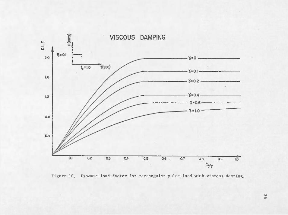
dynamic load factor. Figures 10, 11 and 12 represent maximum dynamic

load factor charts for viscous. Coulomb and structural damping respec­

tively for variations in damping with a rectangular pulse load.

P

Po

o

0 < t /T < 1 — o —

Figure 9. Rectangular pulse load.

25

D.LF

VISCOUS DAMPING

2.0

0.8

0.4

02 04 05 0.7 08 0.9to.

Figure 10. Dynamic load factor for rectangular pulse load with viscous damping.

N)

COULOMB DAMPING

2.0

/ I *0.2

0.4

0.60.8

0.4

02 0.4 0.5 0.6 0.7 0.8 0.9V-

Figure 11. Dynamic load factor for rectangular pulse load with Coulomb damping.

NO

STRUCTURAL DAMPING

G=02j0

G=o.a

G=0.8

0.8

0.4

0.2 0.3 0.4 0.60l5 0.7 OB OB

Figure 12. Dynamic load factor for rectangular pulse load with structural damping.

rooo

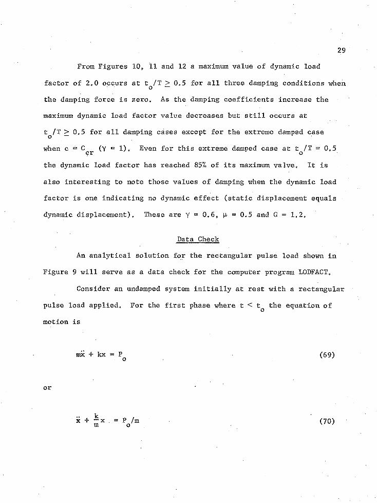
29From Figures 10, 11 and 12 a maximum value of dynamic load

factor of 2.0 occurs at t /T > 0 . 5 for all three damping conditions when

the damping force is zero. As the damping coefficients increase the

maximum dynamic load factor value decreases but still occurs at

t /T > 0 . 5 for all damping cases except for the extreme damped case

when c = (Y = 1). Even for this extreme damped case at £ /T = 0.5

the dynamic load factor has reached 85% of its maximum valve. It is

also interesting to note those values of damping when the dynamic load

factor is one indicating no dynamic effect (static displacement equals

dynamic displacement). These are Y = 0.6, p, = 0.5 and G = 1.2.

Data Check

An analytical solution for the rectangular pulse load shown in

Figure 9 will serve as a data check for the computer program LODFACT.

Consider an undamped system initially at rest with a rectangular

pulse load applied. For the first phase where t < t the equation of

motion is

mx + kx = Pq (69)

or '

x + — x . = P /m (70)m o ' '

Using the relation for circular frequency (Equation 10) gives

2x + (Dx = F

The solution for Equation 71 is of the form

x = I cos 0)t + J sin oat + P /ko

With initial conditions of x(0) = x(0) = 0, Equation 72 becomes

x = P /k(l - cos (tit) o

Expressing Equation 73 in terms of dynamic load factor gives

Df " P^Tk = ^ “ cos tot)O

Using the relationship

(ti = 2nf ® 2tt/T

Equation 74 becomes

D f = (1 - cos 2nt/T)

31

Taking the derivative with respect to t gives

f)f = I 2 sin 2Tit/T (77)

Solving for the maximum dynamic load factor

* 9ttDf = 0 = — sin 2rrt/T (78)

To satisfy Equation 78 t/T = 1/2. From Equation 76 the maximum dynamic

load factor becomes

D fmax = 2 for t J H > 1/2 (79)

For the second phase where t > tQ the equation of motion is

mx + kx = 0 (80)

or

The solution for equation 81 is of the form

x = G cos cut* + H sin cot* (82)

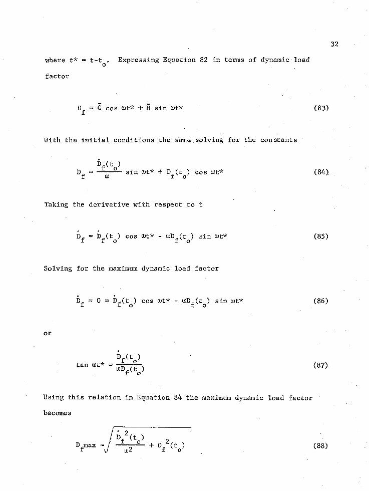
where t* = Expressing Equation 82 in terms of dynamic load

factor

Df = G cos tt)t* 4- H sin (JDt* (83)

With the initial conditions the same.solving for the constants

Df(to)D_ = ------- sin cot* + D (t ) cos cot* (84)t 0) t o

Taking the derivative with respect to t

Dj. = D (t ) cos U)t* - (Jt)D (t ) sin cat* (85)r f o f o

Solving for the maximum dynamic load factor

= 0 = D^(t^) cos cot* - coD^t^) sin cot* (86)

or

Df o^ tan u,t* - Ito ^ T )

Using this relation in Equation 84 the maximum dynamic load factor

becomes

33Using the expression developed for (Equation 76) and (Equation 77)

from phase one. Equation 88 reduces to

/ 2 2 1 D-max =,/ sin wt + (1 - 2 cos cut + cos (tit ) (89)f V o o o

or

D_max = / 2 - 2 cos (tit (90)f V o

Using the trigonometric identity

sin | - y - — I2-— (91)

Equation 90 reduces to

(titoD^max = 2 sin — (92)

Using the expression co = 2rr/T gives

rrtD f = 2 sin ~y - for t^/T < 1/2 (93)

In Figures 10, 11 and 12 plots of dynamic load factor versus

t^/T, the curve representing zero damping follows equations 79 and 93

precisely.

Triangular Pulse Load

For the triangular pulse load shown in Figure 13 values of t

ranging from 0 to 4 were required to give an adequate representation

the maximum dynamic load factor.

P

Po

to

Figure 13. Triangular pulse load.

35

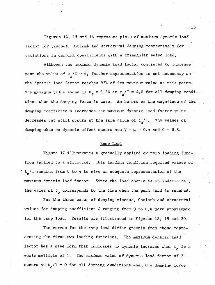
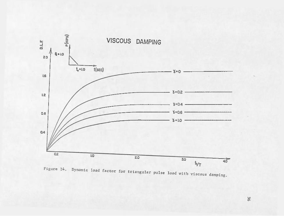
Figures 14, 15 and 16 represent plots of maximum dynamic load

factor for viscous. Coulomb and structural damping respectively for

variations in damping coefficients with a triangular pulse load.

Although the maximum dynamic load factor continues to increase

past the value of t^/T = 4, further representation is not necessary as

the dynamic load factor reaches 93% of its maximum value at this point.

The maximum value shown is = 1,86 at t^/T = 4,0 for all damping condi­

tions when the damping force is zero. As before as the magnitude of the

damping coefficients increases the maximum dynamic load factor value

decreases but still occurs at the same value of t /T. The values ofodamping when no dynamic effect occurs are Y = p s 0,4 and 0 = 0 , 8 ,

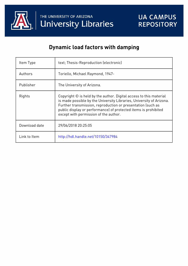
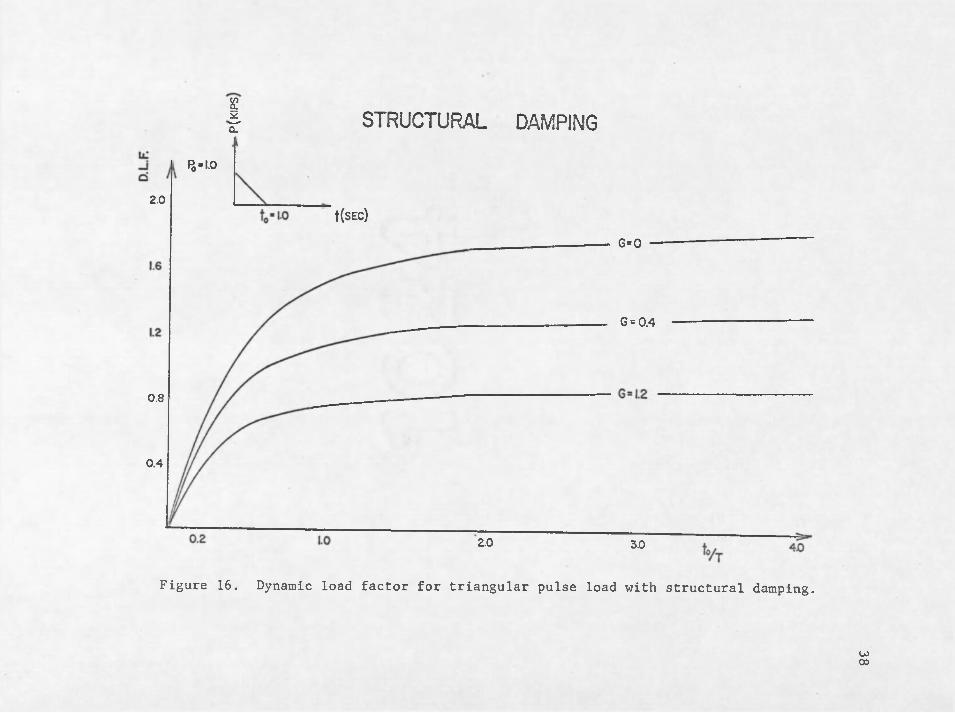
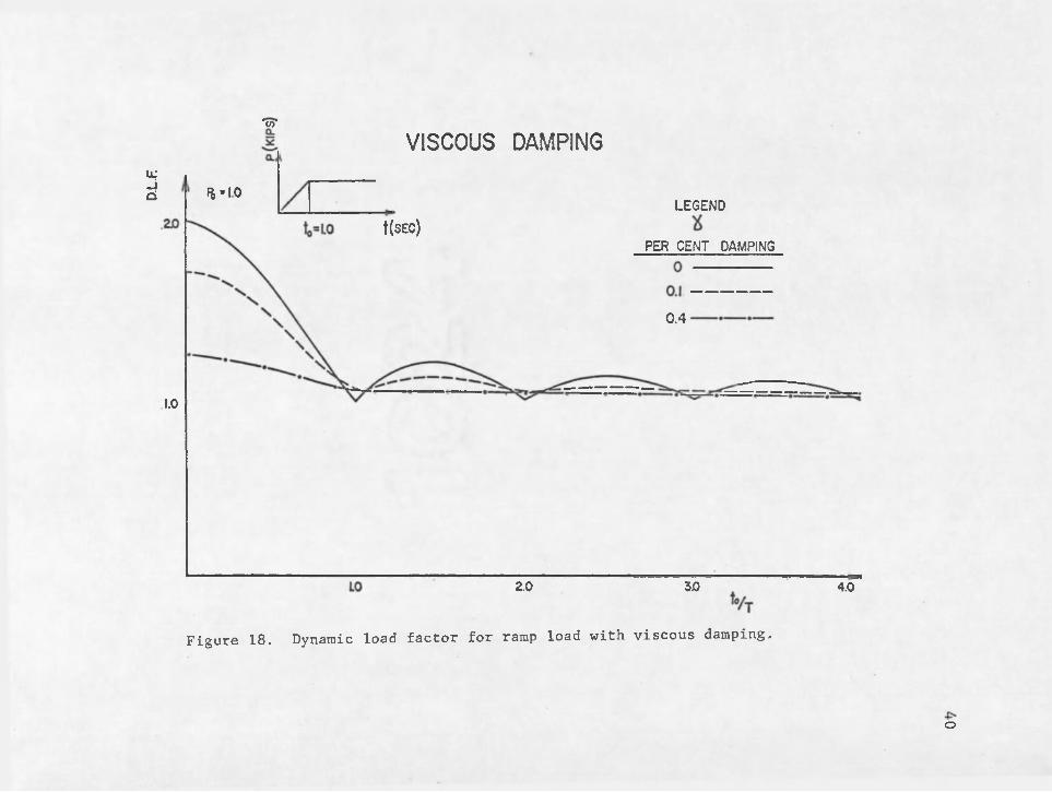
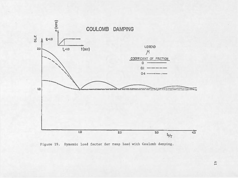
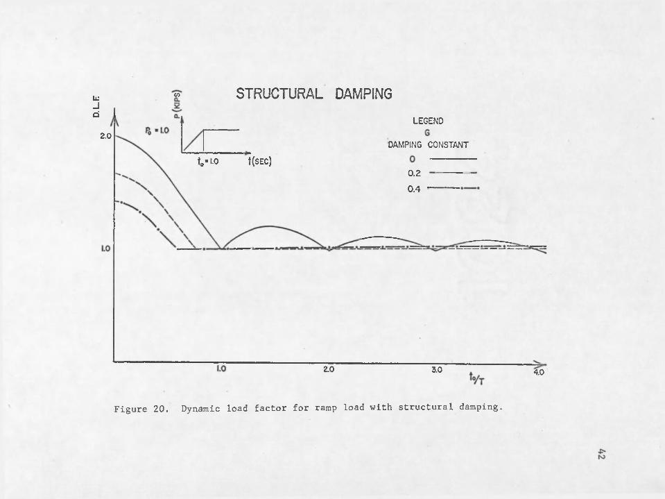
Ramp Load

Figure 17 illustrates a gradually applied or ramp loading func­

tion applied to a structure. This loading condition required values of

t^/T ranging from 0 to 4 to give an adequate representation of the

maximum dynamic load factor. Since the load continues on indefinitely

the value of t^ corresponds to the time when the peak load is reached.

For the three cases of damping viscous, Coulomb and structural

values for damping coefficient G ranging from 0 to 0.4 were programmed

for the ramp load. Results are illustrated in Figures 18, 19 and 20.

The curves for the ramp load differ greatly from those repre­

senting the first two loading functions. The maximum dynamic load

factor has a wave form that indicates no dynamic increase when t is aowhole multiple of T. The maximum value of dynamic load factor of 2

occurs at t /T = 0 for all damping conditions when the damping force

CO

VISCOUS DAMPING

■ 1.02.0

0.8

02ao 3.0

Figure 14. Dynamic load factor for triangular pulseload with viscous damping.

U)

COULOMB DAMPING

2.0

to=IJO t(sEC)

0.8

JX * 0.60.4

0220 3.0 4.0

Figure 15. Dynamic load factor for triangular pulse load with Coulomb damping.

u>'vj

| STRUCTURAL DAMPING

5 -1.0

2.0t(SEC)

G=0

G = 0.4

0.8

0.4

2.0 3.0

Figure 16. Dynamic load factor for triangular pulse load with structural damping.

u>00

39

0 < t /T < 4P

Po

o

Figure 17. Ramp load.

D.L.F

'to*

VISCOUS DAMPING

%"I0LEGEND

t(SEC)PER CENT DAMPING

0.4

1.0

2.0 30 4.0

Figure 18. Dynamic load factor for ramp load with viscous damping.scousVI

o

COULOMB DAMPINGLUa

LEGENDI(s e c)20 t=i.o

COEFFICIENT OF FRICTION

0.4

20 40

Figure 19. Dynamic load factor for ramp load with Coulomb damping.

D.LF

STRUCTURAL DAMPINGco

LEGEND2.0

DAMPING CONSTANTt(SEC)to-1.0

0.20.4

2.0 3.0 4.0

Figure 20. Dynamic load factor for ramp load with structural damping.

43

is zero. When any type of damping is applied the dynamic load factor

reaches a constant value of approximately 1,0 at t /T = 1,0 indicating

no appreciable dynamic effect.

CHAPTER 5

SUMMARY AND CONCLUSIONS

From the nine dynamic load factor charts developed the follow­

ing conclusions are made,

1, Damping may reduce the dynamic response significantly even for

short impulse type loads. When the damping force is large

enough the dynamic response can be reduced below the reference

static response for a given loading function.

2, The duration of a particular load, t , and the period of theostructure, T, are important factors in relation to dynamic

response. Depending on the type of load function the ratio of

t^/T can be very critical for design considerations. For load­

ing functions that are instantaneously applied (rectangular

pulse, and triangular pulse) for a long duration the dynamic

response will be a maximum for the type damping considered,

3, Viscous damping and structural damping have very similar effects

for each loading function studied when the structural damping

coefficient G is twice the percent critical viscous damping.

44

APPENDIX A

NOTATION

Symbol Explanation

A Variable used in calculating acceleration

B Variable used in calculating acceleration

b Constant used in calculating acceleration for° Coulomb damping

b Constant used in calculating acceleration for struc-S tural damping

b Constant used in calculating acceleration for viscousv damping

c Viscous damping coefficient

C Critical dampingcrD Variable used to determine direction of Coulomb dampingC force

Dynamic Load Factor

D Variable used to determine direction of structurals damping force

Coulomb damping force

f Frequency

Fg Structural damping force

F^ Viscous damping force

G Structural damping coefficient

g Gravitational force

45

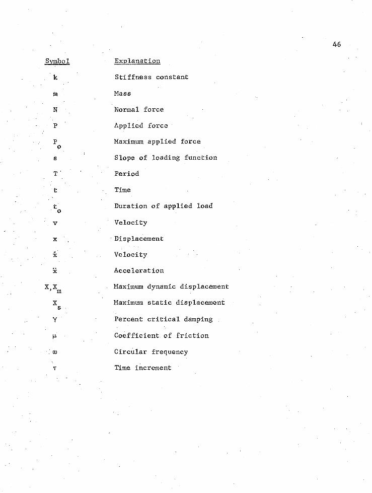
Symbol Explanation

k Stiffness constant

m Mass

N Normal force

P Applied force

P Maximum applied forceQs Slope of loading function

T Period

t Time

Duration of applied load

v Velocity

x ( Displacement

x Velocity

x Acceleration

X,X^ Maximum dynamic displacement

X Maximum static displacementsY Percent critical damping

[A Coefficient of friction

. a) Circular frequency

t Time increment

REFERENCES

Biggs, J. M . , Hansen, R. J., Holley, M. J., Jr., Minami, J. K. , Namye t, S., and Norris, C. H. 1959. Structural Design for Dynamic Loads. New York: McGraw-Hill.

Clough, R. W . , and Penzien, J. 1975. Dynamics of Structures. New York: McGraw-Hill.

Hinkle, R. T., Morse, I. E,, and Tse, F. S. 1963. Mechanical Vibra­tions. Boston: Allyn and Bacon.

Myklestad, N. 0. 1956. Fundamentals of Vibration Analysis. New York:McGraw-Hill,

Thomson, W. T. 1953. Mechanical Vibration. New York: Prentice-Hall.

47