
Factors of Production, Productivity, Institutions and ... · Factors of Production, Productivity,...
20
1 Factors of Production, Productivity, Institutions and Development in Brazil Ana Elisa Gonçalves Pereira* Luciano Nakabashi** Área 2: Desenvolvimento Econômico ABSTRACT Understanding the variables that determine income level and how they are related to each other is critical, particularly because of its importance for planning economic policies. The economic growth and development literature emphasizes that investments in technology, physical and human capital are essential to achieve high levels of development. Political and economic institutions have also been pointed out as relevant features in this process. Employing a sample of 5,507 Brazilian municipalities, this study carries out a development accounting exercise and measures the effect of institutions on per capita Gross Domestic Product (GDP), physical capital intensity, human capital stock and productivity. The empirical results illustrate that differences in the institutional framework are relevant to explain income disparities observed among the Brazilian municipalities. They also indicate that the effects of institutions on GDP occur mainly through human capital stock and total factor productivity and that institutions’ importance is greater for larger municipalities. Key-words: Income Level; Development Accounting; Institutions RESUMO Entender quais são as variáveis relevantes na determinação da renda de uma economia e de que forma essas variáveis se relacionam é fundamental, sobretudo como forma de embasar políticas futuras. A literatura ressalta que o investimento em capital físico, capital humano e tecnologia são essenciais para atingir níveis elevados de desenvolvimento. Tem-se ressaltado, também, a importância das instituições políticas e econômicas sólidas neste processo. Tendo isso em vista, este artigo realiza uma contabilidade do produto dos municípios brasileiros e procura mensurar o efeito da qualidade das instituições sobre o produto e seus componentes (intensidade de capital físico, estoque de capital humano e produtividade), pelo método de Mínimos Quadrados em Dois Estágios, a fim de evitar a possível causalidade reversa entre instituições e desenvolvimento. Os resultados empíricos indicam que as instituições são relevantes na determinação dos díspares níveis de produto per capita municipal e que este efeito ocorre, sobretudo, via produtividade total de fatores e via estoque de capital humano. Há evidências, também, de que o efeito positivo das instituições seja mais expressivo nos municípios mais populosos. Palavas-chave: Nível de Produto; Fatores de Produção; Instituições. JEL: C13; O11; O43. * Doutoranda em Economia pela Escola de Economia de São Paulo – Fundação Getúlio Vargas (EESP- FGV). Endereço eletrônico: [email protected] ** Professor na Universidade de São Paulo, Ribeirão Preto (FEA-RP/USP) e pesquisador do CNPQ. Endereço eletrônico: [email protected]
Transcript of Factors of Production, Productivity, Institutions and ... · Factors of Production, Productivity,...

1
Factors of Production, Productivity, Institutions and Development in Brazil
Ana Elisa Gonçalves Pereira*
Luciano Nakabashi**
Área 2: Desenvolvimento Econômico
ABSTRACT
Understanding the variables that determine income level and how they are related to each other is
critical, particularly because of its importance for planning economic policies. The economic growth
and development literature emphasizes that investments in technology, physical and human capital are
essential to achieve high levels of development. Political and economic institutions have also been
pointed out as relevant features in this process. Employing a sample of 5,507 Brazilian municipalities,
this study carries out a development accounting exercise and measures the effect of institutions on per
capita Gross Domestic Product (GDP), physical capital intensity, human capital stock and productivity.
The empirical results illustrate that differences in the institutional framework are relevant to explain
income disparities observed among the Brazilian municipalities. They also indicate that the effects of
institutions on GDP occur mainly through human capital stock and total factor productivity and that
institutions’ importance is greater for larger municipalities.
Key-words: Income Level; Development Accounting; Institutions
RESUMO
Entender quais são as variáveis relevantes na determinação da renda de uma economia e de que forma
essas variáveis se relacionam é fundamental, sobretudo como forma de embasar políticas futuras. A
literatura ressalta que o investimento em capital físico, capital humano e tecnologia são essenciais para
atingir níveis elevados de desenvolvimento. Tem-se ressaltado, também, a importância das instituições
políticas e econômicas sólidas neste processo. Tendo isso em vista, este artigo realiza uma
contabilidade do produto dos municípios brasileiros e procura mensurar o efeito da qualidade das
instituições sobre o produto e seus componentes (intensidade de capital físico, estoque de capital
humano e produtividade), pelo método de Mínimos Quadrados em Dois Estágios, a fim de evitar a
possível causalidade reversa entre instituições e desenvolvimento. Os resultados empíricos indicam que
as instituições são relevantes na determinação dos díspares níveis de produto per capita municipal e
que este efeito ocorre, sobretudo, via produtividade total de fatores e via estoque de capital humano. Há
evidências, também, de que o efeito positivo das instituições seja mais expressivo nos municípios mais
populosos.
Palavas-chave: Nível de Produto; Fatores de Produção; Instituições.
JEL: C13; O11; O43.
* Doutoranda em Economia pela Escola de Economia de São Paulo – Fundação Getúlio Vargas (EESP-
FGV).
Endereço eletrônico: [email protected]
** Professor na Universidade de São Paulo, Ribeirão Preto (FEA-RP/USP) e pesquisador do CNPQ.
Endereço eletrônico: [email protected]
2
1 INTRODUCTION
Studying and understanding the main causes of economic development differences is one of the
main objectives of economists. Although the concept of development has been expanded over the years
in order to capture the welfare of societies in a broader sense, there is a relative agreement in the
economic literature that high level of output per capita, even if not the sole social welfare determinant,
enables countries, regions and municipalities to achieve a higher living standard and to promote social
welfare. Understanding which are the relevant variables in determining a region income level and how
these variables are related is crucial, especially to provide a framework for economic policies.
The literature that addresses the issues related to economic growth and development emphasizes
that investment in physical capital, human capital and technology is essential to achieve high income
levels. It has also been emphasized the importance of solid economic and political institutions in this
process. By shedding light on the interactions among these variables, we can better understand the
mechanisms through which institutions are able to contribute to raise societies’ living standards.
The vast majority of theoretical and empirical studies in the economic growth and development
literature is built upon a production function. Therefore, it is natural to imagine that the fundamental
variables that affect the output per capita level of an economy operate through their impact on the
accumulation of factors of production and productivity. A sum of recent studies points to institutional
quality as a central variable in this analysis and finds strong evidence that institutions can account for
much of the variation in per capita income across economies. However, institutions by themselves do
not generate product. If institutions are able to explain a significant amount of output level variation
among economies, it shall be via their effects on factors of production accumulation and productivity.
Pande and Udry (2006) investigate the relationship between institutions and development using
intra-country data. They claim that, since macro institutions are constant in intra-country data study, the
results are more reliable and can bring new insights. It is also important to focus the analysis in
developing country case studies because institutions are more important to explain differences in
developing countries income when compared to developed ones, as indicated by Eicher and Leukert
(2009) and Lee and Kim (2009). Lee and Kim (2009)’s results point to the importance of institutions
mainly for low to middle income countries. As a country upgrade to the high income group, factors as
tertiary education and technology innovation became more relevant.
In this scenario, the present study aims to investigate the role of institutions on factors of
production accumulation as well as on total factor productivity in order to understand the channels
through which institutions can influence long-term economic development in the Brazilian
municipalities. To perform the empirical analysis, it is considered the institutions endogeneity problem
in relation to economic performance. This problem can be circumvented by employing the Two Stages
Least Squares (2SLS) method by means of historical and geographical instruments that are
determinants of initial institutions, as applied by previous literature (Acemoglu et. al, 2001; Cavalcanti
et. al., 2008; Easterly and Levine, 2003; Eicher and Leukert, 2009; Engerman and Sokoloff, 2002;
Jones and Hall, 1999; Nakabashi et. al, 2013).
The results indicate that the quality of the Brazilian municipal institutions affect their level of
output per capita mainly via total factor productivity (TFP) and human capital accumulation. In
addition, the institutional quality indicator has a different impact on product, human capital and TFP
when distinct population size samples are considered. Institutions are relevant in all samples, but its
importance increases with the municipalities’ population size.
The remainder of this paper is organized as follows: section two reviews the previous literature
on this subject; the following section describes the data and methodology employed; in the fourth
section it is presented and discussed the empirical results; and the last section concludes.
3
2 INSTITUTIONS, INCOME LEVEL, AND FACTORS OF PRODUCTION
North (1991) defines institutions as the rules of the game in a society, by ensuring property
rights, providing incentives for investment, better or worse wealth and income distribution, political
power, human capital, promoting innovation, and efficient allocation of resources. For the author,
countries’ institutional framework evolution throughout history influenced the amount of productive
investments, it can be regarded as crucial to their different growth trajectories.
Engermann and Sokoloff (2002) also highlight the institutional framework as a fundamental
factor for economic growth and, therefore, long run income level. They propose that in more egalitarian
societies with better institutions, there is greater investment in education, and the increasing levels of
schooling can trigger changes that lead to economic growth, as higher labor productivity, faster
technological innovation and greater participation of people in economic and political activities. The
authors argue that the income level disparities among former European colonies in America are due to
institutional disparities. For them, factor endowments and initial conditions - such as soil, climate,
population size and density of natives - were crucial to determine the type of institutions that initially
developed in these societies.
Some colonies, such as the Caribbean and Brazil, enjoyed climate and soil conditions extremely
favorable to the production of crops that were highly valued in the international market and more
efficiently produced on large scale plantations with slave labor (such as sugar, coffee and tobacco).
Therefore, there was large influx of African slaves to these regions, enabling economies of scale in the
commodities production. The widespread slavery in these regions contributed to unequal income,
human capital, and political power distributions, and consequently to the development of institutions
that benefited a small elite at the majority of the population expense (called extractive institutions by
Acemoglu, Johnson and Robinson, 2002). Engerman and Sokoloff (2002) claim that the impact of
climate and soil on income occurs exclusively via institutions, contrary to some previous studies that
attribute a direct impact of geographical features and initial factor endowment on the level of
development (Bloch, 1988; Lewis, 1978; Pomeranz, 2000; White, 1962; Wrigley, 1988, cited by
Acemoglu et. al., 2002).
Acemoglu et al. (2001, 2002) also link initial institutions to the economic development process.
As Engerman and Sokoloff (2002), they admit a possible reverse causality between institutions and
income level - i.e., regions with higher income levels are more likely to promote better institutions. To
address this problem, they employ instrumental variables related to the initial institutions.
The authors emphasize the institutional inertia hypothesis under which institutions tend to
remain fairly constant over long periods of time. Thus, it is assumed that the factors that led to a
society’s initial institutions development are good instruments for the current ones. Acemoglu et al.
(2002) argue that even extractive institutions - defined as those that concentrate power in the hands of a
small elite, reducing investment, industrialization opportunities, and economic growth - that cause
negative effects on economic development tend to persist over time. Such institutions benefit the elite
who hold political power and therefore the elite has no incentive to change them. Interactions between
de jure and de facto political power explains why the cluster of economic institutions remained
relatively constant in Latin America even with a set of relevant changes in political institutions after
independence, for example (Acemoglu and Robinson, 2008).
Based on the inertia of institutions premise, Acemoglu et al. (2001) employ the potential
mortality rate of colonizers as an instrumental variable for the quality of current institutions. They
believe that this rate (resulting ultimately from geographical conditions) was the major determinant of
the number of European settlers in the various colonized regions. For them, the number of European
settlers was decisive to the formation of initial institutions.

4
Based on data of 332 regions in 16 countries in the Americas, Bruhn and Gallego (2012) find
that the regions more densely populated in the pre-colonial period and that were colonized with bad
colonial activities have a lower level of economic development.1 Easterly and Levine (2003) also found
a statistically significant impact of institutions on output level. Their cross-country results do not give
support to the geography hypothesis. Factor endowments as well as government policies have no direct
influence on economic performance when taking into consideration the effect of institutions.
Arbiaa et. al. (2010) obtain results for the Europeans countries indicating that institutions and
geography are important variables to explain the variations in their productivity, but their results also
indicate that institutions play a dominant role over geographic characteristics, what is consistent with
the findings of Rodrik et. al. (2004) for a worldwide sample of countries.
Some studies that address the relationship between institutions and product level in Brazil are
those performed by Menezes-Filho et al. (2006), Nakabashi et al. (2013), Naritomi (2007), and
Naritomi et al. (2009). Menezes-Filho et al. (2006) find evidences that institutions indeed have an
important role in explaining disparities among the Brazilian states’ GDP per capita. As a proxy for
current institutions’ quality, Menezes-Filho et al. (2006) use a measure of labor laws enforcement. The
authors utilize as proxies for past institutions a number of past variables that have a strong correlation
with current institutions’ quality: the proportion of illiterates, the proportion of voters and the
proportion of foreigners. As the southernmost states had a lower proportion of illiterates, larger number
of electoral colleges and a greater proportion of foreign immigrants, latitude is the most strongly
correlated variable with these past institutional proxies. They used this variable as an instrument to
avoid the reverse causality problem.
To expand the sample size and, consequently, achieve more reliable results from a statistical
perspective, Naritomi (2007) employs a Brazilian municipalities’ database. The author emphasizes the
fact that there is uniformity in the municipalities’ macro-institutions - they have the same political
system, speak the same language - so the achieved results can bring new perspectives. In the empirical
analysis, Naritomi (2007) uses variables such as land distribution, concentration of political power,
management capability, and access to justice to measure institutional quality. She considers two
historical episodes as exogenous sources of institutional variation: the cycles of sugar cane and gold.
Thus, the author attempts to identify the effects of local institutions on economic performance without
incurring on the endogeneity problem. The 2SLS results indicate an important and robust role of
institutions - instrumented by historical variables - in determining the Brazilian municipalities’ GDP
per capita. However, taking these historical episodes as instruments can be a limitation because it is
assigned the same institutional index value for the municipalities that have not integrated these cycles.
The direct use of tools such as latitude, temperature and ethnic fragmentation may provide a
clearer picture of initial institutions developed in each municipality, as proposed by the majority of
empirical analyses that address this subject (Acemoglu et .al., 2005, 2002, 2001; Easterly and Levine,
2003; Eicher and Leukert, 2009; Engerman and Sokoloff, 2002; Hall and Jones, 1999).
Nakabashi et al. (2013) also make use of a database composed by the Brazilian municipalities.
They adopt as instrumental variables geographical and historical features such as latitude, climate and
ethnic fragmentation. The authors find a positive and significant impact of institutional quality -
measured by the Municipal Institutional Quality Index (MIQI) - on the Brazilian municipalities’ GDP.
Cavalcanti et al. (2008) consider data from different institutional features to build an
institutional quality index for a cross-section of countries with emphasis on the Brazilian economy in
the empirical analysis. Their index is based on regulatory costs of “doing private business”, and their
results indicate that these kind of institutions are relevant to determine income per capita.
1 Bad colonial activities are agriculture plantations involving slavery and other forms of coerced labor such as sugar, cotton,
rice and tobacco. They measure economic development based on current income level and on poverty rates.
5
A central study relating institutions and economic development was developed by Hall and
Jones (1999). They employ a sample of 127 countries and attempt to explain the observed difference in
their levels of output per worker. They assert that countries reach high levels of production when they
have high rates of investment in physical and human capital and when they use these inputs
productively. Among the above mentioned studies, this is the first one that evaluates the influence of
institutions on income level through their effects on the factors of production and productivity. Rodrik
et al. (2004) also investigate the effects of institutions on income level, factors of production (physical
and human capital) and total factor productivity in a cross-country sample. The 2SLS regressions
denote that geography has at best weak direct effects on GDP per capita. The results suggest that the
great influence of geography on the income level is via institutional quality, and the impact of
institutions on physical capital accumulation is more expressive than on human capital.
Although there are a significant number of studies that relate institutions and income level,
there are still scarce studies that address this relationship within a country and that underline the
possible transmission channels through which institutions affect income level. The present paper
analyzes the interaction between the two above cited variables in the case of the Brazilian
municipalities as in Nakabashi et al. (2013), and it goes further attempting to identify and to measure
the importance of the indirect effects that institutions have on income per capita through factors of
production accumulation and higher productivity.
3 METHODOLOGY AND DATA
This empirical analysis is based on Hall and Jones (1999)’s methodology. The income level
differences among Brazilian municipalities are decomposed into their factors of production and
productivity. Then, it is estimated the impact of municipal institutions on GDP per capita and its
components. Assume a Cobb-Douglas production function with constant returns to scale:
Yi = Ki(AiHi)
1- (1)
where Yi, Ai, Ki and Hi denote, respectively, the level of output, Harrod-neutral productivity, physical
capital stock, and human capital stock in the municipality i. Dividing both sides of equation (1) by Li -
labor force in municipality i -, we obtain on its left side, GDP per worker. Considering that Y = Yα Y
(1-α)
and dividing both sides of equation (1) by L(1-α)
, facilitates the algebraic manipulation:
Yiα Yi
(1-α)/Li
(1-α) = Ki
α (Ai H
i)(1-α)
/Li(1-α)
(2)
Using lowercase letters to represent the variables in per capita terms2 and rearranging equation
(2), it becomes:
yi(1-α)
= (Ki/Yi )α (Ai hi)
(1-α) (3)
where
y ≡ Y/L; k ≡ K/L; h ≡ H/L (4)
Raising both sides of equation (3) to the 1⁄(1-α) power:
yi = (Ki/Yi)(α/(1-α)
(Ai hi)(1-α)
(5)
Equation (5) decomposes output per capita into the three mentioned components. Hall and
Jones (1999) indicate that it is better to use capital-output ratio instead of capital-labor ratio because if
there is an exogenous increase in productivity, the K/L ratio will grow over time. In other words, if we
used capital-labor ratio in the product decomposition, its growth reflecting increases in productivity
2 In the empirical analysis, the municipalities’ population will be used as a proxy for their workforce. Therefore, the term
per worker is replaced by per capita hereafter.

6
would be erroneously attributed to capital accumulation. From equation (5), it is possible to decompose
Brazilian municipalities’ output per capita into productivity, capital intensity and human capital per
capita. This decomposition was performed based on a municipal database for 2000.
Data commonly used as proxies for physical capital stock at the Brazilian state level - as the
consumption of non-residential electricity - are not available to all municipalities, so we used urban
residential capital stock as a physical capital proxy. To measure human capital, it was employed the
human capital stock variable from the Brazilian Institute of Applied Economic Research (IPEA).
Productivity is calculated from equation (5) as a residual, as usually done in the development
accounting literature. For the parameter of income share of physical capital, this paper assumes the
value of α = 0.4, as in previous studies using national data (Gomes et. al., 2003; Coelho and Figueiredo,
2007). Taking the natural logarithm of both sides of equation (5), it can be expressed as:
lnyi = α/(1-α) lnKi/Yi + lnhi + lnAi (6)
To avoid the endogeneity problem, it is adopted a variety of geographical and historical
variables as exogenous instruments for municipal institutions and the equations are estimated by the
Two Stages Least Squares (2SLS) method, such as the international and national literature in this area.
This method also mitigates measurement error and relevant variables omission problems.
The econometric specification is:
i) First stage: lnIi = α0 + Z'iλ + X'iδ + μi (7)
ii) Second stage: lnyi = θ0 + θ1lnIi(hat) + X'iβ + ε(1,i) (8)
α/(1-α) lnKi/Yi = θ2 + θ3lnIi(hat)+ X'i γ + ε(2,i) (9)
lnhi = θ4 + θ5lnIi(hat)+X'i φ + ε(3,i) (10)
lnAi = θ6 + θ7lnIi(hat) +X'i + ε(4,i) (11)
where yi is GDP per capita of the municipality i, Ii is a proxy for institutional quality, ki is a proxy for
physical capital per capita, hi is a proxy for human capital per capita, Ai is Total Factor Productivity
(TFP), µi and εi are the error terms, Zi is a vector of instrumental variables, and Xi is a vector of other
exogenous control variables (included to test the robustness of the institutional quality proxy
coefficient). To estimate equations (8) to (11) by 2SLS, it is necessary that the instruments in Z vector
from equation (7) exhibit the desirable properties: to have high correlation with the endogenous
explanatory variables and to be orthogonal to the error terms.
We adopt geographical features as instruments for institutions such as latitude and climate
(considered determinants of initial institutions), ethnic fractionalization and proportion of whites (as
proxies for the type of colonization that occurred in each municipality, affecting initial institutions). It
is also assumed that institutions are persistent through time as argued by Acemoglu and Robinson
(2008, 2006). In this scenario, variables that are related to the establishment of initial institutions
capture the effect of current institutions on income and factors of production accumulation, avoiding
the endogeneity problem.
There is a significant correlation between latitude and current institutional proxy, which is
probably due to the fact that the establishment of Brazilian municipalities’ initial institutions was
related to the type of colonization and to the initial economic activities. In the north of the country,
which is warmer and more suitable for sugar cane cultivation, for example, there was a predominance
of large-scale plantations with slavery, and the production was directed to foreign markets. The
7
literature emphasizes that this system of production is historically linked to the emergence of
institutions unfavorable to subsequent economic development (Engerman and Sokoloff, 2002).
Following this reasoning, another candidate for the municipalities’ instrumental variables is the
proportion of people of European descent. Many authors employ variables that reflect the influence of
Western Europe - considered the birthplace of "good institutions" - as instruments for institutional
quality. Hall and Jones (1999), for example, use as instrumental variables linguistic aspects of the
population to capture the extent to which countries have been influenced by Western Europe, the first
region in the world to implement a social infrastructure favorable to production. The reasoning of
Acemoglu et al. (2002) is similar. The authors assert that in regions where European settlers established
in greater numbers, it was more likely to be developed the so-called private property institutions that
favored industrialization and the development process, unlike the extractive institutions, which favor
the concentration of power in the hands of small elite and reduce the economic growth opportunities. In
the present paper, based on this reasoning, it is used as a proxy for the presence of good institutions the
proportion of whites in each of the Brazilian municipalities.
In fact, among the potential instruments, the two variables that presented higher correlations
with the institutional quality indicator were the distance from the equator (0.59) and the proportion of
whites (0.54). These variables are in the Z vector in equation (7) in most of the estimated regressions to
circumvent the reverse causality problem between institutions and economic performance. For
comparison purposes, we have used temperature and the ethnic fractionalization index as instruments in
some of the first stage regressions. They have correlations of -0.51 and -0.26, respectively, with the
institutional quality index. Alesina et al. (2003) find a negative correlation between their ethnic
fractionalization index and institutions. The ethnic fragmentation index was calculated following
Mauro’s (1995) methodology, with data from the Brazilian Census (IBGE). The index is constructed
according to:
frac = 1 - ∑(nj/N)2 (12)
where nj is the number of individuals belonging to group j and N≡∑nj is the total number of
individuals. The five categories are: white (European descendants), mixed (pardos), black (African
descendants), yellow (East Asian descendants) and indigenous (natives). As this indicator increases, the
municipality’s ethnic fractionalization rises.
To measure institutional quality, it is employed the Municipal Institutional Quality Index
(MIQI) elaborated by the Brazilian Ministry of Planning, Budget and Management in 2005, based on
the Survey of Basic Municipal Information of 1999 from the Brazilian Bureau of Statistics (IBGE),
Appendix A provides a full description of this index. Besides the institutional index, some regressions
include control variables as the Gini inequality index, the municipalities’ degree of urbanization, the
municipality's age, the distance from the state capital, and altitude. Appendix B provides a detailed
description of the variables used in the empirical analysis and their data sources.
4 EMPIRICAL RESULTS
Initially, we present the estimated results employing the Brazilian municipalities’ full sample,
and the results that exclude the municipalities considered to be outliers. Then, municipalities are
divided into samples according to their population size. The first table in this section displays the
effects of the institutional quality indicator on the log of per capita GDP and on its components - the
three additive terms of equation (6). Thus, the sum of columns (2), (3), and (4) coefficients yields the
first column coefficient, and the sum of columns (6), (7), and (8) coefficients yields column (5)

8
coefficient. Regressions from (1) to (4) are based on the municipalities’ full sample, while the estimates
from columns (5) through (8) are based on the sample without the outliers3.
TABLE 1: 2SLS Estimates (instruments: llat lpropwhite) Whole Sample Without Outliers
Explained Variable Explained Variable (1) (2) (3) (4) (5) (6) (7) (8)
lny ∝/(1-∝)
lnk/y lnh lnA
lny ∝/(1-∝)
lnk/y Lnh lnA
4.3275 0.1349 1.3792 2.8133 4.3092 0.1431 1.3793 2.7868 (0.0998)*** (0.0561)** (0.0317)*** (0.1124)*** (0.0979)*** (0.0555)*** (0.0318)*** (0.1088)***
const. -3.5910 -0.3552 1.6611 -4.8969 -3.5827 -0.3571 1.6608 -4.8864 (0.1119)*** (0.0616)*** (0.0354)*** (0.1251)*** (0.1098)*** (0.0606)*** (0.0354)*** (0.1211)***
Obser. 5503 5503 5503 5503 5470 5470 5470 5470 F 1880.63 5.74 1889.29 626.24 1937.31 6.65 1886.48 656.27
Prob>F 0.000 0.016 0.000 0.000 0.000 0.010 0.000 0.000
DWH a 943.451 11.072 897.768 269.635 1021.182 10.030 896.189 306.258
(p-value) 0.0000 0.0009 0.0000 0.0000 0.0000 0.0015 0.0000 0.0000
Hansen J b 1.855 6.389 0.405 0.022 1.146 9.434 0.468 0.454
(p-value) 0.1732 0.0115 0.5245 0.8827 0.2844 0.0021 0.4938 0.5004
ACC LR c 2231.219 2231.219 2231.219 2231.219 2226.644 2226.644 2226.644 2226.644
(p-value) 0.0000 0.0000 0.0000 0.0000 0.0000 0.0000 0.0000 0.0000
S.Y. d 1374.958 1374.958 1374.958 1374.958 1373.314 1373.314 1373.314 1373.314
Ho a 10 % 19.93 19.93 19.93 19.93 19.93 19.93 19.93 19.93 Source: Authors’ elaboration.
Notes: Asterisks indicate statistical significance: *** significant at 1%; ** significant at 5%; * significant at 10%. Heteroskedasticity-
consistent standard errors are in parentheses. MIQI was instrumented in the first stage by latitude and proportion of whites. a: Durbin-Wu-
Hausman test for endogeneity. A rejection of H0 indicates the MIQI should be treated as an endogenous variable. b: J Hansen test for the
instruments quality (alternative to Sargan test when it is reported robust standard errors). The rejection of H0 casts doubt on the
instruments validity. c: Anderson Canonical Correlation test. The rejection of H0 indicates that the equation is identified. d: Cragg-Donald
F statistic and Stock and Yogo critical value. The rejection of H0 indicates the absence of weak instruments. GDP per capita is represented
by y, k/y is the capital-output ratio, h is a proxy for human capital per capita, A represents total factor productivity, and MIQI is the
municipal institutional quality index. Const. is the intercept, Obser. is the number of observations, and F statistic tests the joint
significance of the estimated coefficients.
In column (1), we observe the estimated impact of the institutional quality index on the
municipalities’ output per capita. The MIQI coefficient is positive and significant at the 1% level. Since
the variables are in log, the coefficients can be interpreted as elasticities: a 1% improvement in the
institutional quality corresponds to a 4.33% municipal output per capita average increase.
The last four rows of Table 1 report the tests results for endogeneity and for the validity and
relevance of the instruments in the first stage regressions. In all regressions, the Durbin-Wu-Hausman
tests rejected the null hypothesis of MIQI exogeneity, indicating that this index should be treated as
endogenous, i.e. it is appropriate to use the 2SLS method to estimate de regressions. The Hansen J test -
similar to the Sargan test, however for heteroskedasticity consistent standard errors - tests the joint null
hypothesis that: i) the instruments are valid (uncorrelated with the error term), and ii) the excluded
instruments are correctly excluded (i.e., the instrumental variables enter just in the first stage, having no
direct effects on the dependent variable in the second stage). This test does not reject the null
hypothesis in regression (1), indicating that latitude and proportion of whites’ instruments are valid (not
correlated with the residuals) and that they have no direct impact on output per capita. The Anderson
Canonical Correlation statistic tests the null hypothesis that the equation is unidentified. In all
regressions in Table 1, H0 is rejected, indicating that the instruments are relevant (correlated with the
endogenous regressor). It is also necessary to test whether the instruments are weak. The Cragg-Donald
3 The list of municipalities excluded from the sample in these regressions is in Appendix C.

9
statistic is used to check it. In all regressions in this table, the null hypothesis that the instruments are
weakly correlated with the endogenous regressor is rejected.
In column (2), the dependent variable is the first component of the production function on the
right-hand side of equation (6). Because the log of physical capital intensity is multiplied by α/(1- α)
and α = 0.4, to interpret the MIQI coefficient in the second column as elasticity, it is necessary to
multiply it by a factor of 1.5. Taking this into consideration, we can observe that municipalities with
1% better institutions have, on average, 0.2% higher capital intensity, and this effect is significant at
5%. However, in addition to the small impact of institutions on capital intensity, the Hansen J statistic
rejects the null hypothesis of the instruments validity, affecting the results reliability.
Column (3) reports the estimation results with log h as the left-hand side variable. The impacts
of institutions on human capital are more substantial. The results suggest that a 1% increase in the
institutional quality proxy has a positive impact of 1.38% in per capita human capital. The coefficient is
significant at 1% level, and in this column, the Hansen J statistic indicates that the instruments are
valid. The other tests also indicate that the instruments are not weak.
In Table 1 fourth regression, the dependent variable is the log of Total Factor Productivity
(TFP). Although MIQI coefficient is statistically significant and has positive effects on output and on
its three decomposition components, its effect on productivity is higher than on the other two product
components. The estimated parameter indicates that a 1% improvement in the institutional quality
indicator is related to a 2.81% average increase on TFP.
The remaining results in the four last columns of Table 1 are based in a sample reduced in 33
municipalities, which had discrepant values of product per capita (usually small municipalities that host
large companies, mining companies, refineries, etc.). The results changes marginally with their
exclusion. The estimated coefficients values changed slightly, and the tests results and estimated
parameters statistical significance remained unchanged (the exception is the significance level of the
capital intensity coefficient, which increased from 5% to 1%).
The following table has been included in order to test the results’ robustness, i.e. to see what
happens to the estimated coefficients and their standard deviations when other control variables are
included. Again, columns (1) to (4) results are based on the full sample of Brazilian municipalities,
while the remaining columns are based on the sample without the 33 above mentioned outliers.
TABLE 2: 2SLS results - control variables (instruments: llat and lpropwhite) Whole sample
Without outliers
Dependent variable Dependent variable (1) (2) (3) (4) (5) (6) (7) (8)
lny ∝/(1-∝)
lnk/y lnh lnA
lny ∝/(1-∝)
lnk/y lnh lnA
3.9640 -0.6573 1.1429 3.4784 3.9611 -0.6579 1.1427 3.4763 (0.1091)*** (0.0510)*** (0.0305)*** (0.1315)*** (0.1070)*** (0.0490)*** (0.0305)*** (0.1266)***
Gini -0.3837 -0.3627 -0.1565 0.1355 -0.3624 -0.3775 -0.1585 0.1737
(0.1852)** (0.0870)*** (0.0512)*** (0.2282) (0.1838)** (0.0854)*** (0.0513)*** (0.2245)
Urban 0.7335 0.9540 0.4099 -0.6304 0.7026 0.9761 0.4113 -0.6848
(0.0464)*** (0.0242)*** (0.0129)*** (0.0586)*** (0.0453)*** (0.0231)*** (0.0130)*** (0.0558)***
Age -0.0037 0.0054 0.0005 -0.0096 -0.0037 0.0053 0.0005 -0.0096
(0.0005)*** (0.0003)*** (0.0001)*** (0.0007)*** (0.0005)*** (0.0002)*** (0.0001)*** (0.0006)***
distcapital -1.87e-05 -1.44e-04 5.79e-06 1.19e-04 -4.06e-05 -1.33e-04 3.84e-06 8.90e-05
(6.21e-05) (2.94e-05)*** (1.80e-05) (7.71e-05) (6.07e-05) (2.80e-05)*** (1.81e-05) (7.37e-05)
Altitude -4.04e-05 1.36e-04 -1.14e-05 -1.65e-04 -3.53e-05 1.32e-04 -1.18e-05 -1.55e-04 (3.35e-05) (1.69e-05)*** (9.35e-06) (4.26e-05)*** (3.27e-05) (1.61e-05)*** (9.40e-06) (4.07e-05)***
const. -3.2516 -0.0691 1.7486 -4.9310 -3.2520 -0.0654 1.7499 -4.9365 (0.1729)*** (0.0799) (0.0498)*** (0.2071)*** (0.1710)*** (0.0782) (0.0498)*** (0.2027)***
Obser. 5503 5503 5503 5503 5470 5470 5470 5470
F 457.53 562.04 785.98 191.17 462.98 609.51 784.66 212.44

10
Prob>F 0.000 0.000 0.000 0.000 0.000 0.000 0.000 0.000
DWH a 828.812 40.030 943.176 339.518 897.519 51.379 939.186 389.748
(p-value) 0.0000 0.0000 0.0000 0.0000 0.0000 0.0000 0.0000 0.0000
Hansen J b 1.071 5.527 0.194 0.035 0.562 9.663 0.318 0.528
(p-value) 0.3006 0.0187 0.6594 0.8510 0.4534 0.0019 0.5731 0.4674
ACC LR c 1568.586 1568.586 1568.586 1568.586 1564.865 1564.865 1564.865 1564.865
(p-value) 0.0000 0.0000 0.0000 0.0000 0.0000 0.0000 0.0000 0.0000
S.Y. d 906.175 906.175 906.175 906.175 904.509 904.509 904.509 904.509
Ho a 10 % 19.93 19.93 19.93 19.93 19.93 19.93 19.93 19.93 Source: Authors’ elaboration.
Notes: Asterisks indicate statistical significance: *** significant at 1%; ** significant at 5%; * significant at 10%. Heteroskedasticity-
consistent standard errors are in parentheses. MIQI was instrumented in the first stage by latitude and proportion of whites. a: Durbin-Wu-
Hausman test for endogeneity. A rejection of H0 indicates the MIQI should be treated as an endogenous variable. b: J Hansen test for the
instruments quality (alternative to Sargan test when it is reported robust standard errors). The rejection of H0 casts doubt on the
instruments validity. c: Anderson Canonical Correlation test. The rejection of H0 indicates that the equation is identified. d: Cragg-Donald
F statistic and Stock and Yogo critical value. The rejection of H0 indicates the absence of weak instruments. GDP per capita is represented
by y, k/y is the capital-output ratio, h is a proxy for human capital per capita, A represents total factor productivity, and MIQI is the
municipal institutional quality index. Gini index of inequality is the Gini index of income inequality, urban is the degree of urbanization,
age is the municipality years from its emancipation to the 2000 year, distcapital is the municipality distance from the State capital in
kilometers, and altitude is the altitude in meters. Const. is the intercept, Obser. is the number of observations, and F statistic tests the joint
significance of the estimated coefficients.
The control variables insertion did not invalidate the conclusions of the MIQI impacts on
product per capita, but the regressions with the product components as the left hand-side variable
changed considerably. A 1% rise in MIQI is reflected in a 3.96% average GDP per capita change, with
1% level of significance. This effect is somewhat lower than that found in Table 1 (4.33%), in which
MIQI was the only explanatory variable.
The Gini index shows a negative and significant (at 5%) effect on the explained variable,
indicating that municipalities with worse income distribution (higher Gini) have lower per capita
product, ceteris paribus. However, its effect is not substantial in quantitative terms. Since the Gini
index has a standard deviation of 0.059, the estimated parameter implies that one standard deviation
increase in this index reflects in a GDP per capita fall of only 0.02%.
The urbanization degree and municipality’s age variables are also significant at 1% level. 1%
more urbanized municipalities have, on average, 0.73% higher income per capita, ceteris paribus. The
age variable effect is small: 100 years younger municipalities have only a 0.37% average higher
income per capita, taking into consideration the other variables influence. The distance from the state
capital and altitude are not statistically significant on output per capita level determination.
The most altered results after the control variables inclusion are those in which the explained
variable is the physical capital intensity. In column (2) of Table 2, it is possible to note that the MIQI
coefficient sign is reversed in relation to the results presented in the same column of Table 1. The MIQI
coefficient suggests that better institutions are associated with lower capital intensity.4 If, indeed, the
effect of MIQI on capital intensity is negative, a possible explanation is that of Hall, Sobel and Crowley
(2010). For the authors, where institutions are weak, a relevant part of physical capital is employed in
rent-seeking and other unproductive activities. If this is the case, controlling for other variables, one
can expect that where institutions are stronger, the capital stock is used more efficiently. Pritchett
(2000) also stresses that poorer regions with weaker institutions are more likely to overestimate
physical capital investments because part that is recorded as investment is diverted into other uses.
Therefore, poorer regions have recorded higher stocks of physical capital than in reality.
Also in column (2), we can verify that the Gini index is significant and has the expected sign
(municipalities with worse income distribution have lower physical capital intensity). Urbanization
4 This result could stem from the fact that the physical capital proxy is correlated with the urbanization degree variable
(correlation of 0.57), but this possibility is ruled out because estimating the same regression without the urbanization degree
variable, the negative sign and significance of the coefficient remains.

11
degree and the municipality age have a positive influence on the capital-output ratio. The variable
distance to the state capital is also significant, and its negative sign suggests that municipalities closer
to the state capitals are more capital-intensive, ceteris paribus. Altitude has a positive and significant
effect on the explained variable. However, all results in column (2) should be interpreted with caution
since the Hansen J test rejects (at least at 5% significance level) the validity of the instruments.
Regression (3) dependent variable is the (log) human capital per capita stock. The MIQI
coefficient is significant at 1% and indicates that municipalities with 1% better institutions have 1.14%
higher human capital per capita. The inclusion of the controls does not alter this variable significance,
but its quantitative effect is reduced to approximately 83% of its prior effect (Table 1).
The Gini index influence is negative and significant, indicating that income distribution affects
the Brazilian municipalities’ output per capita also via human capital accumulation. This effect is
consistent with the literature that emphasizes the role of better income distribution in fostering
investment in education (Engermann and Sokoloff, 2002). Urbanization degree has a positive and
significant effect on the explained variable. 1% more urbanized municipalities have, on average, a
0.41% higher human capital per capita stock. Another significant variable is the municipality’s age.
Older municipalities have higher stocks of human capital, keeping everything else constant. Finally, the
results indicate that the variables distance from the state capital and altitude are not relevant on human
capital per capita determination.
In the fourth column of this table, the explained variable is log Total Factor Productivity (TFP).
The log MIQI estimated coefficient in column (4) indicates that 1% better institutions are associated
with 3% higher TFP. This result is also in line with the literature (Arbiaa, Battistib and Di Vaio, 2010).
Good institutions encourage innovation. In addition, better institutions tend to allocate productive
resources more efficiently. This effect of institution on TFP seems to be even more important in
relation to human capital accumulation for the Brazilian municipalities.
The Gini index seems to have no effect on TFP. The sign of the urbanization degree is the
opposite of the previous regressions and this effect is significant at 1% level. The municipalities’ age
variable has a negative and significant influence on TFP. Altitude also has a negative impact on TFP.
Combining the effects of urbanization degree and altitude on TFP, we can interpret that in Brazil,
predominantly rural and plane municipalities (probably based on agriculture) have relatively higher
productivity, ceteris paribus. In the remaining results of Table 3 - columns (5) to (8) - the explanatory
variables estimated coefficients are similar in magnitude and significance level to the prior results,
indicating that the results almost do not change with the exclusion of the outliers.5
The significance and magnitude of the municipal institutions quality coefficient are not
considerably altered with the use of alternative instruments instead of latitude: temperature and ethnic
fragmentation index. However, the Hansen J test indicates them as not valid instruments, and therefore
these results are not reported here. The tests indicate that the use of llat and lpropwhite in previous
regressions were indeed the most appropriate choice.
Table 3 reports the results of estimating the institutional quality indicator influence on output
per capita when the sample is separated by municipalities’ population size. The objective of this
procedure is to assess if the effects of institutions on output per capita level are different according to
the municipalities’ population size. The hypothesis is that municipalities with larger population have
more coordination problems, more difficulties to solve their collective problems based on trust, and
therefore institutions are more relevant in their development process. For comparison purpose, the first
column of Table 3 replicates column (1) results of Table 2. Columns (2) to (6) display the estimations’
results based on different samples. In the last column, the sample is composed by 224 municipalities
with population over 100 thousand inhabitants.
5 In the next tables, the reported results are the ones based on the full sample because the results are quite similar when the
outliers are excluded from the database.
12
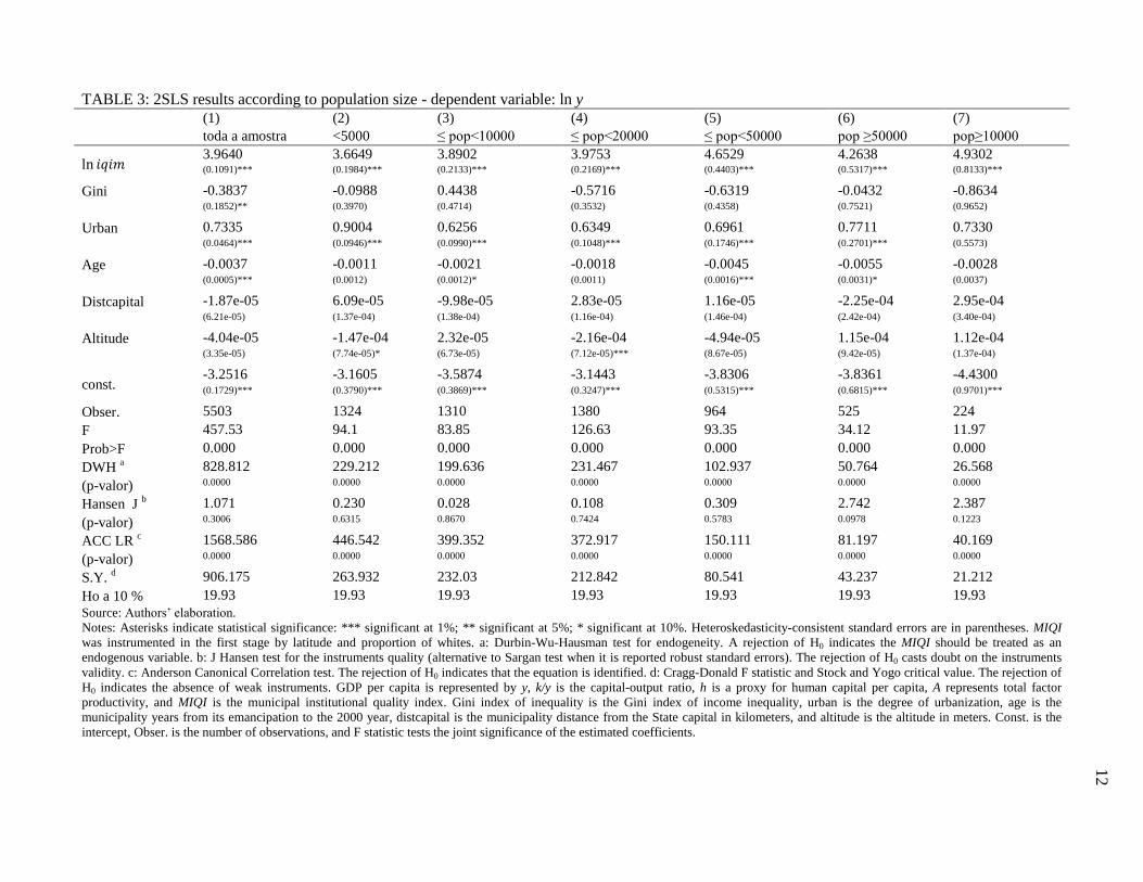
TABLE 3: 2SLS results according to population size - dependent variable: ln y
(1) (2) (3) (4) (5) (6) (7)
toda a amostra <5000 ≤ pop<10000 ≤ pop<20000 ≤ pop<50000 pop ≥50000 pop≥10000
3.9640 3.6649 3.8902 3.9753 4.6529 4.2638 4.9302 (0.1091)*** (0.1984)*** (0.2133)*** (0.2169)*** (0.4403)*** (0.5317)*** (0.8133)***
Gini -0.3837 -0.0988 0.4438 -0.5716 -0.6319 -0.0432 -0.8634
(0.1852)** (0.3970) (0.4714) (0.3532) (0.4358) (0.7521) (0.9652)
Urban 0.7335 0.9004 0.6256 0.6349 0.6961 0.7711 0.7330
(0.0464)*** (0.0946)*** (0.0990)*** (0.1048)*** (0.1746)*** (0.2701)*** (0.5573)
Age -0.0037 -0.0011 -0.0021 -0.0018 -0.0045 -0.0055 -0.0028
(0.0005)*** (0.0012) (0.0012)* (0.0011) (0.0016)*** (0.0031)* (0.0037)
Distcapital -1.87e-05 6.09e-05 -9.98e-05 2.83e-05 1.16e-05 -2.25e-04 2.95e-04
(6.21e-05) (1.37e-04) (1.38e-04) (1.16e-04) (1.46e-04) (2.42e-04) (3.40e-04)
Altitude -4.04e-05 -1.47e-04 2.32e-05 -2.16e-04 -4.94e-05 1.15e-04 1.12e-04
(3.35e-05) (7.74e-05)* (6.73e-05) (7.12e-05)*** (8.67e-05) (9.42e-05) (1.37e-04)
const. -3.2516 -3.1605 -3.5874 -3.1443 -3.8306 -3.8361 -4.4300 (0.1729)*** (0.3790)*** (0.3869)*** (0.3247)*** (0.5315)*** (0.6815)*** (0.9701)***
Obser. 5503 1324 1310 1380 964 525 224
F 457.53 94.1 83.85 126.63 93.35 34.12 11.97
Prob>F 0.000 0.000 0.000 0.000 0.000 0.000 0.000
DWH a 828.812 229.212 199.636 231.467 102.937 50.764 26.568
(p-valor) 0.0000 0.0000 0.0000 0.0000 0.0000 0.0000 0.0000
Hansen J b 1.071 0.230 0.028 0.108 0.309 2.742 2.387
(p-valor) 0.3006 0.6315 0.8670 0.7424 0.5783 0.0978 0.1223
ACC LR c 1568.586 446.542 399.352 372.917 150.111 81.197 40.169
(p-valor) 0.0000 0.0000 0.0000 0.0000 0.0000 0.0000 0.0000
S.Y. d 906.175 263.932 232.03 212.842 80.541 43.237 21.212
Ho a 10 % 19.93 19.93 19.93 19.93 19.93 19.93 19.93
Source: Authors’ elaboration.
Notes: Asterisks indicate statistical significance: *** significant at 1%; ** significant at 5%; * significant at 10%. Heteroskedasticity-consistent standard errors are in parentheses. MIQI
was instrumented in the first stage by latitude and proportion of whites. a: Durbin-Wu-Hausman test for endogeneity. A rejection of H0 indicates the MIQI should be treated as an
endogenous variable. b: J Hansen test for the instruments quality (alternative to Sargan test when it is reported robust standard errors). The rejection of H0 casts doubt on the instruments
validity. c: Anderson Canonical Correlation test. The rejection of H0 indicates that the equation is identified. d: Cragg-Donald F statistic and Stock and Yogo critical value. The rejection of
H0 indicates the absence of weak instruments. GDP per capita is represented by y, k/y is the capital-output ratio, h is a proxy for human capital per capita, A represents total factor
productivity, and MIQI is the municipal institutional quality index. Gini index of inequality is the Gini index of income inequality, urban is the degree of urbanization, age is the
municipality years from its emancipation to the 2000 year, distcapital is the municipality distance from the State capital in kilometers, and altitude is the altitude in meters. Const. is the
intercept, Obser. is the number of observations, and F statistic tests the joint significance of the estimated coefficients.
13
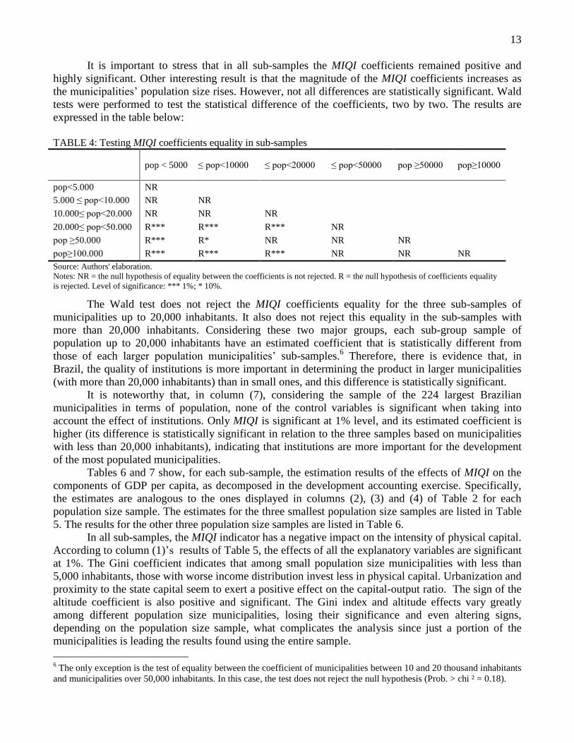
It is important to stress that in all sub-samples the MIQI coefficients remained positive and
highly significant. Other interesting result is that the magnitude of the MIQI coefficients increases as
the municipalities’ population size rises. However, not all differences are statistically significant. Wald
tests were performed to test the statistical difference of the coefficients, two by two. The results are
expressed in the table below:
TABLE 4: Testing MIQI coefficients equality in sub-samples
pop < 5000 ≤ pop<10000 ≤ pop<20000 ≤ pop<50000 pop ≥50000 pop≥10000
pop<5.000 NR
5.000 ≤ pop<10.000 NR NR
10.000≤ pop<20.000 NR NR NR
20.000≤ pop<50.000 R*** R*** R*** NR
pop ≥50.000 R*** R* NR NR NR
pop≥100.000 R*** R*** R*** NR NR NR
Source: Authors' elaboration.
Notes: NR = the null hypothesis of equality between the coefficients is not rejected. R = the null hypothesis of coefficients equality
is rejected. Level of significance: *** 1%; * 10%.
The Wald test does not reject the MIQI coefficients equality for the three sub-samples of
municipalities up to 20,000 inhabitants. It also does not reject this equality in the sub-samples with
more than 20,000 inhabitants. Considering these two major groups, each sub-group sample of
population up to 20,000 inhabitants have an estimated coefficient that is statistically different from
those of each larger population municipalities’ sub-samples.6 Therefore, there is evidence that, in
Brazil, the quality of institutions is more important in determining the product in larger municipalities
(with more than 20,000 inhabitants) than in small ones, and this difference is statistically significant.
It is noteworthy that, in column (7), considering the sample of the 224 largest Brazilian
municipalities in terms of population, none of the control variables is significant when taking into
account the effect of institutions. Only MIQI is significant at 1% level, and its estimated coefficient is
higher (its difference is statistically significant in relation to the three samples based on municipalities
with less than 20,000 inhabitants), indicating that institutions are more important for the development
of the most populated municipalities.
Tables 6 and 7 show, for each sub-sample, the estimation results of the effects of MIQI on the
components of GDP per capita, as decomposed in the development accounting exercise. Specifically,
the estimates are analogous to the ones displayed in columns (2), (3) and (4) of Table 2 for each
population size sample. The estimates for the three smallest population size samples are listed in Table
5. The results for the other three population size samples are listed in Table 6.
In all sub-samples, the MIQI indicator has a negative impact on the intensity of physical capital.
According to column (1)’s results of Table 5, the effects of all the explanatory variables are significant
at 1%. The Gini coefficient indicates that among small population size municipalities with less than
5,000 inhabitants, those with worse income distribution invest less in physical capital. Urbanization and
proximity to the state capital seem to exert a positive effect on the capital-output ratio. The sign of the
altitude coefficient is also positive and significant. The Gini index and altitude effects vary greatly
among different population size municipalities, losing their significance and even altering signs,
depending on the population size sample, what complicates the analysis since just a portion of the
municipalities is leading the results found using the entire sample.
6 The only exception is the test of equality between the coefficient of municipalities between 10 and 20 thousand inhabitants
and municipalities over 50,000 inhabitants. In this case, the test does not reject the null hypothesis (Prob. > chi ² = 0.18).

14
TABLE 5: 2SLS results by municipalities’ population size – production function components (three smallest population sample size) (1) (2) (3) (4) (5) (6) (7) (8) (9)
pop<5000 5000≤ pop<10000 1000≤ pop<20000
∝/(1-∝)
lnk/y lnh lnA
∝/(1-∝)
lnk/y Lnh lnA
∝/(1-∝)
lnk/y lnh lnA
-0.6807 1.0178 3.3278 -0.5907 1.0543 3.4266 -0.5718 1.0452 3.5019 (0.0992)*** (0.0562)*** (0.2452)*** (0.0924)*** (0.0558)*** (0.2499)*** (0.1001)*** (0.0571)*** (0.2624)***
Gini -0.5477 -0.1197 0.5686 -0.7428 -0.1984 1.3850 -0.2328 -0.2629 -0.0759
(0.1989)*** (0.1095) (0.5096) (0.2100)*** (0.1188)* (0.5696)** (0.1690) (0.0875)*** (0.4422)
Urban 1.0762 0.3586 -0.5345 0.9837 0.3208 -0.6789 0.9559 0.3827 -0.7037
(0.0513)*** (0.0263)*** (0.1238)*** (0.0504)*** (0.0257)*** (0.1260)*** (0.0503)*** (0.0260)*** (0.1295)***
Age 0.0060 0.0015 -0.0086 0.0061 0.0014 -0.0096 0.0048 0.0011 -0.0077
(0.0006)*** (0.0003)*** (0.0016)*** (0.0006)*** (0.0003)*** (0.0015)*** (0.0005)*** (0.0003)*** (0.0014)***
Distcapital -4.06e-04 1.46e-05 4.52e-04 -2.00e-04 5.26e-06 9.48e-05 -1.21e-04 4.65e-05 1.03e-04 (6.66e-05)*** (3.73e-05) (1.70E-04)*** (6.57e-05)*** (3.77e-05) (1.74e-04) (5.26e-05)** (3.57e-05) (1.41e-04)
Altitude 9.76e-05 -5.39e-05 -1.91e-04 9.72e-05 -1.11e-05 -6.28e-05 1.95e-04 -4.60e-05 -3.65e-04 (4.48e-05)** (2.07e-05)*** (1.06e-04)* (3.30e-05)*** (1.80e-05) (8.38e-05) (3.41e-05)*** (1.76e-05)*** (8.97e-05)***
const. 0.0604 1.9060 -5.1270 0.0746 1.8913 -5.5533 -0.2196 1.8926 -4.8173 (0.1876) (0.1081)*** (0.4722)*** (0.1666) (0.1030)*** (0.4495)*** (0.1573) (0.0822)*** (0.4054)***
Obser. 1324 1324 1324 1310 1310 1310 1380 1380 1380
F 193.60 121.66 77.32 131.45 170.95 48.05 113.44 222.09 36.71 Prob>F 0.000 0.000 0.000 0.000 0.000 0.000 0.000 0.000 0.000
DWH a 34.089 231.561 117.968 11.488 232.607 93.968 11.244 251.733 97.720
(p-value) 0.0000 0.0000 0.0000 0.0007 0.0000 0.0000 0.0008 0.0000 0.0000
Hansen J b 1.732 0.088 0.719 1.573 0.003 0.124 3.724 0.195 1.215
(p-value) 0.1881 0.7666 0.3965 0.2098 0.9564 0.7250 0.0536 0.6587 0.2704
ACC LR c 446.542 446.542 446.542 399.352 399.352 399.352 372.917 372.917 372.917
(p-value) 0.0000 0.0000 0.0000 0.0000 0.0000 0.0000 0.0000 0.0000 0.0000
S.Y. d 263.932 263.932 263.932 232.03 232.03 232.03 212.842 212.842 212.842
Ho a 10 % 19.93 19.93 19.93 19.93 19.93 19.93 19.93 19.93 19.93 Source: Authors’ elaboration.
Notes: Asterisks indicate statistical significance: *** significant at 1%; ** significant at 5%; * significant at 10%. Heteroskedasticity-consistent standard errors are in parentheses. MIQI
was instrumented in the first stage by latitude and proportion of whites. a: Durbin-Wu-Hausman test for endogeneity. A rejection of H0 indicates the MIQI should be treated as an
endogenous variable. b: J Hansen test for the instruments quality (alternative to Sargan test when it is reported robust standard errors). The rejection of H0 casts doubt on the instruments
validity. c: Anderson Canonical Correlation test. The rejection of H0 indicates that the equation is identified. d: Cragg-Donald F statistic and Stock and Yogo critical value. The rejection of
H0 indicates the absence of weak instruments. GDP per capita is represented by y, k/y is the capital-output ratio, h is a proxy for human capital per capita, A represents total factor
productivity, and MIQI is the municipal institutional quality index. Gini index of inequality is the Gini index of income inequality, urban is the degree of urbanization, age is the
municipality years from its emancipation to the 2000 year, distcapital is the municipality distance from the State capital in kilometers, and altitude is the altitude in meters. Const. is the
intercept, Obser. is the number of observations, and F statistic tests the joint significance of the estimated coefficients.

15
TABLE 6: 2SLS Results by Municipalities’ Population Size – Production Function Components (Three Largest Population Samples Size)
(1) (2) (3) (4) (5) (6) (7) (8) (9)
20000≤ pop<50000 pop≥50000 pop≥100000
∝/(1-∝) lnk/y lnh lnA
∝/(1-∝) lnk/y Lnh lnA
∝/(1-∝) lnk/y lnh lnA
-0.5836 1.3177 3.9189 -0.4731 1.5586 3.1783 -0.8431 1.6981 4.0752 (0.1955)*** (0.1136)*** (0.5322)*** (0.2452)* (0.1806)*** (0.6310)*** (0.3864)** (0.2906)*** (1.0053)***
Gini 0.1170 -0.1305 -0.6184 -0.4216 0.5619 -0.1835 -0.6456 0.5270 -0.7449 (0.1785) (0.1308) (0.4814) (0.3355) (0.2251)** (0.8977) (0.4536) (0.2907)* (1.2239)
Urban 0.8580 0.4420 -0.6039 0.9061 0.4677 -0.6027 0.8782 0.3388 -0.4840 (0.0854)*** (0.0446)*** (0.2195)*** (0.1696)*** (0.1141)*** (0.3100)* (0.2706)*** (0.2453) (0.7903)
Idade 0.0042 0.0000 -0.0086 (0.0026 -0.0008 -0.0073 0.0008 -0.0004 -0.0033 (0.0007)*** (0.0004) (0.0019)*** (0.0014)* (0.0011) (0.0036)** (0.0015) (0.0013) (0.0043)
Distcapital -9.56e-05 4.44e-05 6.28e-05 2.03e-05 -2.40e-05 -2.21e-04 -1.60e-04 1.26e-04 (3.30e-04
(6.77e-05) (4.04e-05) (1.78e-04) (1.02e-04) (7.51e-05) (2.80e-04) (1.44e-04) (1.07e-04) (4.07e-04)
Altitude 1.67e-04 1.923-05 -2.36e-04 3.54e-05 2.66e-05 5.30e-05 -1.68e-05 1.61e-05 (1.12e-04
(3.78e-05)*** (2.373-05) (1.03e-04)** (4.54e-05) (3.28e-05) (1.16e-04) (6.05e-05) (5.16e-05) (1.61e-04)
const. -0.3322 1.5086 -5.0071 -0.1034 0.8892 -4.6219 0.6521 0.8193 -5.9014 (0.2135) (0.1508)*** (0.5932)*** (0.3336) (0.2277)*** (0.8176)*** (0.4135) (0.3196)*** (1.2221)***
Obser. 964 964 964 525 525 525 224 224 224 F 59.00 144.50 19.30 7.31 43.01 5.49 3.78 14.10 4.09
Prob>F 0.000 0.000 0.000 0.000 0.000 0.000 0.001 0.000 0.001 DWH
a 1.114 150.875 34.542 0.017 86.601 10.732 0.286 43.719 6.357
(p-value) 0.2913 0.0000 0.0000 0.8955 0.0000 0.0011 0.5928 0.0000 0.0117
Hansen J b 0.005 0.099 0.125 0.353 0.341 1.279 0.007 0.448 1.766
(p-value) 0.9452 0.7532 0.7236 0.5527 0.5591 0.2581 0.9318 0.5035 0.1838
ACC LR c 150.111 150.111 150.111 81.197 81.197 81.197 40.169 40.169 40.169
(p-value) 0.0000 0.0000 0.0000 0.0000 0.0000 0.0000 0.0000 0.0000 0.0000
S.Y. d 80.541 80.541 80.541 43.237 43.237 43.237 21.212 21.212 21.212
Ho a 10 % 19.93 19.93 19.93 19.93 19.93 19.93 19.93 19.93 19.93 Source: Authors’ elaboration.
Notes: Asterisks indicate statistical significance: *** significant at 1%; ** significant at 5%; * significant at 10%. Heteroskedasticity-consistent standard errors are in parentheses. MIQI
was instrumented in the first stage by latitude and proportion of whites. a: Durbin-Wu-Hausman test for endogeneity. A rejection of H0 indicates the MIQI should be treated as an
endogenous variable. b: J Hansen test for the instruments quality (alternative to Sargan test when it is reported robust standard errors). The rejection of H0 casts doubt on the instruments
validity. c: Anderson Canonical Correlation test. The rejection of H0 indicates that the equation is identified. d: Cragg-Donald F statistic and Stock and Yogo critical value. The rejection of
H0 indicates the absence of weak instruments. GDP per capita is represented by y, k/y is the capital-output ratio, h is a proxy for human capital per capita, A represents total factor
productivity, and MIQI is the municipal institutional quality index. Gini index of inequality is the Gini index of income inequality, urban is the degree of urbanization, age is the
municipality years from its emancipation to the 2000 year, distcapital is the municipality distance from the State capital in kilometers, and altitude is the altitude in meters. Const. is the
intercept, Obser. is the number of observations, and F statistic tests the joint significance of the estimated coefficients.
16
In columns (1), (4) and (7) of Table 6, there is the same signal to the institutional quality
coefficient on the determination of k/y ratio as in columns (1), (4) and (7) of Table 5. That is, for all
samples based on distinct population sizes, the institutional indicator has a negative effect on capital
intensity. This effect is not statistically different among the samples in most cases, so we omit the Wald
test results.
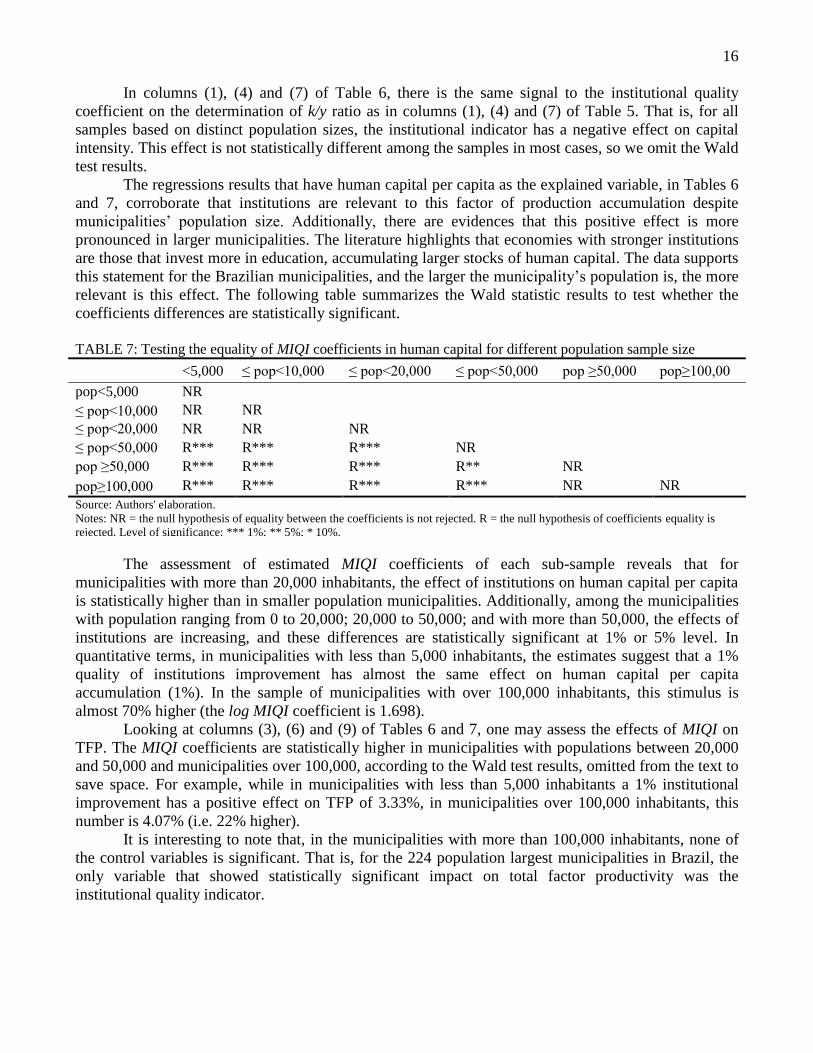
The regressions results that have human capital per capita as the explained variable, in Tables 6
and 7, corroborate that institutions are relevant to this factor of production accumulation despite
municipalities’ population size. Additionally, there are evidences that this positive effect is more
pronounced in larger municipalities. The literature highlights that economies with stronger institutions
are those that invest more in education, accumulating larger stocks of human capital. The data supports
this statement for the Brazilian municipalities, and the larger the municipality’s population is, the more
relevant is this effect. The following table summarizes the Wald statistic results to test whether the
coefficients differences are statistically significant.
TABLE 7: Testing the equality of MIQI coefficients in human capital for different population sample size
<5,000 ≤ pop<10,000 ≤ pop<20,000 ≤ pop<50,000 pop ≥50,000 pop≥100,00
pop<5,000 NR
≤ pop<10,000 NR NR
≤ pop<20,000 NR NR NR
≤ pop<50,000 R*** R*** R*** NR
pop ≥50,000 R*** R*** R*** R** NR
pop≥100,000 R*** R*** R*** R*** NR NR
Source: Authors' elaboration.
Notes: NR = the null hypothesis of equality between the coefficients is not rejected. R = the null hypothesis of coefficients equality is
rejected. Level of significance: *** 1%; ** 5%; * 10%.
The assessment of estimated MIQI coefficients of each sub-sample reveals that for
municipalities with more than 20,000 inhabitants, the effect of institutions on human capital per capita
is statistically higher than in smaller population municipalities. Additionally, among the municipalities
with population ranging from 0 to 20,000; 20,000 to 50,000; and with more than 50,000, the effects of
institutions are increasing, and these differences are statistically significant at 1% or 5% level. In
quantitative terms, in municipalities with less than 5,000 inhabitants, the estimates suggest that a 1%
quality of institutions improvement has almost the same effect on human capital per capita
accumulation (1%). In the sample of municipalities with over 100,000 inhabitants, this stimulus is
almost 70% higher (the log MIQI coefficient is 1.698).
Looking at columns (3), (6) and (9) of Tables 6 and 7, one may assess the effects of MIQI on
TFP. The MIQI coefficients are statistically higher in municipalities with populations between 20,000
and 50,000 and municipalities over 100,000, according to the Wald test results, omitted from the text to
save space. For example, while in municipalities with less than 5,000 inhabitants a 1% institutional
improvement has a positive effect on TFP of 3.33%, in municipalities over 100,000 inhabitants, this
number is 4.07% (i.e. 22% higher).
It is interesting to note that, in the municipalities with more than 100,000 inhabitants, none of
the control variables is significant. That is, for the 224 population largest municipalities in Brazil, the
only variable that showed statistically significant impact on total factor productivity was the
institutional quality indicator.

17
5 CONCLUSIONS
The results of this study employing Brazilian municipal data indicate that the quality of
municipal institutions affects the level of output per capita. After decomposing the product level into its
components via a Cobb-Douglas production function, it was observed that this effect is due to the
positive inducement of institutional quality on total factor productivity (TFP) and on human capital per
capita accumulation. Controlling for the endogeneity of institutions by the Two Stage Least Square
(2SLS) method, the positive effects of institutional quality on productivity, human capital and the level
of output per capita were robust to the inclusion of control variables such as income distribution,
degree of urbanization, altitude and distance from the state capital.
The positive effect of institutions on capital intensity, observed initially, was not robust to the
inclusion of the above mentioned control variables. In many specifications its influence was negative
on physical capital accumulation. Income inequality, measured by the Gini index, presented significant
negative effects on capital intensity in several specifications. The results suggest that municipalities
with more egalitarian income distribution have higher physical capital investment rates.
Another relevant conclusion is that the institutional quality indicator has a different impact on
product, on human capital accumulation and on TFP when it is considered distinct population size
samples. In municipalities with small populations, the institutional quality is important in determining
income per capita level, but this effect is quantitatively less substantial when compared to larger
municipalities. This effect is due to the higher importance of institutions on TFP and, mainly, human
capital determination on more populated municipalities. In particular, the results for the 224 most
populated Brazilian municipalities sample (over 100,000 inhabitants), the institutional quality indicator
was the only significant variable in determining the output per capita level, productivity and human
capital per capita.
There are still many relationships to be explored in more depth, especially regarding the ways in
which institutional quality affects output per capita level and the complex relationship among income
distribution, institutions and factors of production accumulation. With evidences that, in Brazil,
institutions affect the product per capita mainly via human capital accumulation and productivity, we
hope that the present analysis can instigate further research in the area.
REFERENCES
ACEMOGLU, D.; JOHNSON, S.; ROBINSON, J., 2001. The Colonial Origins of Comparative
Development: An Empirical Investigation. American Economic Review, v. 91, p. 1369-1401.
ACEMOGLU, D.; JOHNSON, S.; ROBINSON, J., 2002. Reversal of Fortune: Geography and
Institutions in the Making of the Modern World Income Distribution. Quarterly Journal of Economics,
v. 117, p. 1231-1294.
ACEMOGLU, D.; JOHNSON, S.; ROBINSON, J., 2005. Institutions as the fundamental cause of long-
run growth. In Handbook of Economic Growth, Chapter 6, p. 385–472.
ACEMOGLU, D.; ROBINSON, J., 2006. De Facto Political Power and Institutional Persistence.
American Economic Review PAPERS AND PROCEEDINGS,vol. 96 (2), p. 325-330.
ACEMOGLU, D.; ROBINSON, J., 2008. Persistence of power, elites and institutions. American
Economic Review, vol. 98 (1), p. 267–293.

18
ALESINA, A.; DEVLESCHAWUER, A.; EASTERLY, W.; KURLAT, S.; WACZIARG, R., 2003.
Fractionalization. Journal of Economic Growth, vol. 8 (2), p. 155-94.
ALESINA, A.; PEROTTI, R., 1998. Economic Risk and Political Risk in Fiscal Unions. Economic
Journal, Royal Economic Society, vol. 108 (449), p. 989-1008.
ARBIAA, G.; BATTISTIB, M.; DI VAIO, G., 2010. Institutions and geography: Empirical test of
spatial growth models for European regions. Economic Modelling, vol. 27 (1), p. 12-21.
BRUHN, M.; GALLEGO, F.A., 2012. Good, Bad, and Ugly Colonial Activities: Do They Matter for
Economic Development? The Review of Economic and Statistics, vol. 94 (2), p. 433-461.
CAVALCANTI, T.V.; MAGALHÃES, A.M.; TAVARES, J.A. (2008). Institutions and Economic
Development in Brazil. The Quarterly Review of Economics and Finance, vol. 48, p. 412-432.
COELHO, R.L.P.; FIGUEIRÊDO, L., 2007. Uma Análise da Hipótese de Convergência para os
Municípios Brasileiros. Revista Brasileira de Economia, vol. 61, p. 331-352.
EASTERLY, W.; LEVINE, R., 2003. Tropics, Germs, and Crops: how endowments influence
economic development. Journal of Monetary Economics, vol. 50 (1), p. 3-39.
EICHER. T. S.; LEUKERT, A., 2009. Institutions and Economic Performance: Endogeneity and
Parameter Heterogeneity. Journal of Money, Credit and Banking, vol. 41 (1), p. 197–219.
ENGERMAN, S. L.; SOKOLOFF, K. L., 2002. Factor endowments, inequality and paths of
development among new world economics. National Bureau of Economic Research, Cambridge.
GOMES, V., PESSÔA, S. A., & VELOSO, F., 2003. Evolução da produtividade total dos fatores na
economia brasileira: Uma análise comparativa. Pesquisa e Planejamento Econômico, vol. 33, n. 3, p.
389-434.
HALL, R. E.; JONES, C. I., 1999. Why Do Some Countries Produce So Much More Output per
Worker than Others? Quarterly Journal of Economics, vol. 114, n.1, pp. 83-116.
HALL, J. C.; SOBEL, R.S.; CROWLEY,J. R., 2010. Institutions, Capital, and Growth. Southern
Economic Journal, vol. 77, n. 2, p. 385-405.
LEE, K.; KIM, B. Y., 2009. Both Institutions and Policies Matter but Differently for Different Income
Groups of Countries: Determinants of Long-Run Economic Growth Revisited. World Development,
vol 37 (3), p. 533-549.
MENEZES-FILHO, N.; MARCONDES, R.L.; PAZELLO, E.T.; SCORZAFAVE, L.G., 2006.
Instituições e Diferenças de Renda entre os Estados Brasileiros: Uma Análise Histórica. In: XXXIV
BRAZILIAN ECONOMIC CONGRESS (ENCONTRO NACIONAL DE ECONOMIA), 2006,
Salvador.
MINISTÉRIO DO PLANEJAMENTO, ORÇAMENTO E GESTÃO. Agenda Político-Institucional.
<http://www.planejamento.gov.br/secretarias/upload/Arquivos/spi/downloads/081014_DOWN_EX_P
C_Agen_sumAgenda.pdf>

19
NAKABASHI,L; PEREIRA, A.E.G.; SACHSIDA, A., 2013. Institutions and Growth: A Developing
Country Case Study. Journal of Economic Studies. In press.
NARITOMI, J., 2007. Herança Colonial, Instituições e Desenvolvimento. Master Thesis. Economics
Graduate Program, Pontifícia Universidade Católica do Rio de Janeiro, Rio de Janeiro.
NARITOMI, J.; SOARES, R.; ASSUNÇÃO, J. J., 2009. Institutional Development and Colonial
Heritage within Brazil. Departmento de Economia PUC-Rio, Working Paper, 561.
NORTH, D. C.. Institutions., 1991. Journal of Economic Perspectives, v. 5, n. 1, p. 97-112.
PANDE, R.; UDRY, C., 2006. Institutions and Development: A View from Below. Economic Growth
Center, Yale University (Working paper).
PRITCHETT, L., 2000. The Tyranny of Concepts: CUDIE (Cumulated Depreciated Investment Effort)
is not Capital”. Journal of Economic Growth, vol. 5, p. 361-384.
RAJAN, R.G., 2007. The persistence of Underdevelopment: Constituencies and Competitive Rent
Preservation. ECGI Working Paper Series in Finance, 150.
RODRIK, D.; SUBRAMANIAN, A.; TREBBI, F., 2004. Institutions Rule: The Primacy of Institutions
over Geography and Integration in Economic Development. Journal of Economic Growth, vol. 9, p.
131-165.
STOCK, J.H.; YOGO, M., 2005. Testing for Weak Instruments in Linear IV Regression. In D.W.K.
Andrews and J.H. Stock, eds. Identification and Inference for Econometric Models: Essays in Honor
of Thomas Rothenberg. Cambridge: Cambridge University Press, 2005, pp. 80–108. Working paper
version: NBER Technical Working Paper 284.
APPENDIX A - Description of the institutional quality indicator
FIGURE A.1: Diagram of the institutional quality indicator composition
Degree of
Participation
(33%)
• Existence of councils (4%).
• Councils installed (4%).
• Policy councils (7%).
• Deliberative councils (7%).
• Councils that manage funds (11%).
Financial
Capacity
(33%)
• Existence of consortia (11%).
• Current Revenue vs Debt (11%).
• Real per capita savings (11%).
Management
Capacity
(33%)
• Up-to-dateness values of tax properties (8%).
• Degree of property tax on time payments (8%).
• Management tools (8%).
• Planning tools (8%).
MIQI

20
SOURCE: Brazilian Ministry of Planning, Budge and Management
Notes: The degree of participation measures population participation in local government and it is based on the number of
municipal councils and their characteristics. The financial capacity is based on the number of inter-municipal associations,
the relationship between a municipality’s debt and its current revenues, net of personnel expenses (which reflects the
municipality capacity to repay its debt in time), and real per capita savings. The management capacity is based on the
properties’ up-to-dateness values for tax purposes, the degree of property tax on time payments, and the number of
management and planning tools available to the municipal government. The management tools are: existence of district
administration or administrative regions; subprefecture (it is an administrative division of a municipality that is below
prefecture); master plan (strategic planning); act land; zoning law or equivalent; construction code; and code of postures.
The planning tools are: the existence of government plan; strategic plan and organic law (sort of municipal constitution).
APPENDIX B - Description of variables and data source - TABLE B.1: Description of variables and data source
Variable Description Data Source
Y Gross domestic product in 2000 Brazilian Bureau of Statistics (IBGE)
K Urban residencial capital in 2000 Ipeadata
H Human capital stock in 2000 Ipeadata
L Total resident population in2000 Ipeadata
MIQI Municipal Institutional Quality Indicator
The Brazilian Ministry of Planning, Budget
and Management based on the Survey of
Basic Municipal Information of 1999 from
the Brazilian Bureau of Statistics (IBGE)
Gini Income inequality index in 2000 Ipeadata
Urban Urbanization degree in 2000; Ratio (urban residential
population)/(total residential population)
Authors’ elaboration based on data from
Ipeadata
Distcapital Distance from the State Capital (km) Ipeadata
Altitude Altitude in meters Ipeadata
Age 2000 minus the municipal installation year Authors’ elaboration based on data from
IBGE
Propwhite
Proportion of whites; ratio (population that has declared
themselves as being white in the 2010 census) / total
residential population)
Authors’ elaboration based on data from
2010 IBGE census
Latitude Distance from de equator; latitude absolute value in degrees Ipeadata
Temp Annual average temperature in oC Ipeadata
Frac Ethnic fractionalization index following the methodology of
Mauro (1995)
Authors’ elaboration based on data from
2010 IBGE census
APPENDIX C - Outliers - TABLE C.1: Outliers
Municipality State Municipality State Municipality State
Barcarena PA São João Batista do Glória MG Cubatão SP
Parauapebas PA José da Barra MG Jambeiro SP
Ipojuca PE Tapira MG Luis Antônio SP
Camaçari BA Anchieta ES Motuca SP
São Francisco do Conde BA Carapebus RJ Ouroeste SP
Arapora MG Porto Real RJ Sandovalina SP
Betim MG Quissama RJ Taciba SP
Fortaleza de Minas MG Rio das Ostras RJ Triunfo RS
Fronteira MG Ariranha SP Itiquira MT
Indianópolis MG Castilho SP Perolândia GO
Pirajuba MG Colombia SP Sao Simão GO


