FACTORIZATION OF TROPICAL POLYNOMIALS by Nathan...
62
FACTORIZATION OF TROPICAL POLYNOMIALS IN ONE AND SEVERAL VARIABLES by Nathan B. Grigg Submitted to Brigham Young University in partial fulfillment of graduation requirements for University Honors Department of Mathematics Brigham Young University June 2007 Advisor: Tyler Jarvis Signature: Honors Representative: Steve Turley Signature:
-
Upload
hoangkhanh -
Category
Documents
-
view
215 -
download
1
Transcript of FACTORIZATION OF TROPICAL POLYNOMIALS by Nathan...
FACTORIZATION OF TROPICAL POLYNOMIALS
IN ONE AND SEVERAL VARIABLES
by
Nathan B. Grigg
Submitted to Brigham Young University in partial fulfillment
of graduation requirements for University Honors
Department of Mathematics
Brigham Young University
June 2007
Advisor: Tyler Jarvis
Signature:
Honors Representative: Steve Turley
Signature:

Copyright c© 2007 Nathan B. Grigg
All Rights Reserved
ABSTRACT
FACTORIZATION OF TROPICAL POLYNOMIALS
IN ONE AND SEVERAL VARIABLES
Nathan B. Grigg
Department of Mathematics
Bachelor of Science
This paper discusses the theory of factoring tropical polynomials as well
as some factoring techniques. I give an elementary proof of the Fundamen-
tal Theorem of Tropical Algebra and describe an algorithm to factor single-
variable polynomials with rational coefficients. For multi-variable tropical
polynomials I discuss the corner locus and a correspondence between poly-
nomials and weighted balanced complexes. I prove that tropical factorization
is NP-complete, and I give an algorithm that is efficient for many classes of
polynomials.

ACKNOWLEDGMENTS
I would like to thank all of those who have helped with this project. Thanks
to Gretchen Rimmasch for being a good friend and mentor, to Nathan Man-
waring, Natalie Wilde, and Julian Tay for their help, ideas, and support.
Thanks to my advisor, Dr. Jarvis, for making time in his very busy schedule
to help me when I needed it. Also, thanks to the BYU Math Department and
the Office of Research and Creative Activities for providing me with monetary
support.
Most of all, thanks to my Amy for her love, support, and motivation. She
has helped me more (and read this thesis more times) than anyone else that I
know.

Contents
Title and signature page . . . . . . . . . . . . . . . . . . . . . . . . . . . . iAbstract . . . . . . . . . . . . . . . . . . . . . . . . . . . . . . . . . . . . . vAcknowledgements . . . . . . . . . . . . . . . . . . . . . . . . . . . . . . . viiTable of Contents . . . . . . . . . . . . . . . . . . . . . . . . . . . . . . . . ixList of Figures . . . . . . . . . . . . . . . . . . . . . . . . . . . . . . . . . . xi
1 Introduction 11.1 The Rational Tropical Semi-ring . . . . . . . . . . . . . . . . . . . . . 3
2 Tropical Polynomials of One Variable 52.1 Polynomials and Functions . . . . . . . . . . . . . . . . . . . . . . . . 62.2 Least-coefficient Polynomials . . . . . . . . . . . . . . . . . . . . . . . 82.3 The Fundamental Theorem of Tropical Algebra . . . . . . . . . . . . 132.4 The Corner Locus of a Polynomial . . . . . . . . . . . . . . . . . . . 15
3 Tropical Polynomials of Several Variables 193.1 The Corner Locus and Weighted Balanced Complex . . . . . . . . . . 20
3.1.1 The Corner Locus . . . . . . . . . . . . . . . . . . . . . . . . . 203.1.2 The Weighted Balanced Complex . . . . . . . . . . . . . . . . 213.1.3 Polynomial-Complex Correspondence . . . . . . . . . . . . . . 24
3.2 Factors and Balanced Subcomplexes . . . . . . . . . . . . . . . . . . . 263.3 A Factoring Algorithm . . . . . . . . . . . . . . . . . . . . . . . . . . 29
3.3.1 NP-completeness . . . . . . . . . . . . . . . . . . . . . . . . . 293.3.2 A factoring algorithm . . . . . . . . . . . . . . . . . . . . . . . 303.3.3 Analysis . . . . . . . . . . . . . . . . . . . . . . . . . . . . . . 32
4 Conclusion 35
Appendix: The Tropical Maple Package 37
Bibliography 59
v

List of Figures
2.1 Functional equivalence, equality, and least coefficients . . . . . . . . . 72.2 A factoring example . . . . . . . . . . . . . . . . . . . . . . . . . . . 15
3.1 The corner locus of a polynomial in two variables . . . . . . . . . . . 213.2 A weighted balanced 2-complex . . . . . . . . . . . . . . . . . . . . . 243.3 Weighted balanced graph of a product . . . . . . . . . . . . . . . . . 283.4 Decomposing a Newton polyhedron by factoring a tropical polynomial 303.5 A two-variable factoring example . . . . . . . . . . . . . . . . . . . . 33
vi

Chapter 1
Introduction
Tropical algebra, also called “min-plus” or “max-plus” algebra, is a relatively new
topic in mathematics that has recently caught the interest of algebraic geometers,
computer scientists, combinatorists, and other mathematicians. According to An-
dreas Gathmann [5], tropical algebra was pioneered by mathematician and computer
scientist Imre Simon in the 1980s but did not receive widespread attention until a few
years ago. Interestingly, the title “tropical algebra” is nothing more than a reference
to Simon’s home country—Brazil.
Tropical algebra is a useful tool in solving a wide variety of problems. For example,
it can be used to solve complicated phylogenetic problems [2, 14], to simplify mathe-
matical physics problems [8], and to study implications of statistical models [11]. In
addition, tropical algebra often provides an easier way to solve complex enumerative
geometry problems [6, 10]. It can even be used to find and assess algorithms for
solving the classic traveling salesman problem [1].
The tropical semi-ring, which is the basis of this problem-solving tool and our
major object of study, is formed by replacing the standard addition operation with
the minimum function and replacing multiplication with addition (see Definition 1).
1

2
Although many difficult problems can be translated into simpler tropical problems,
even these simpler problems can be difficult if we do not understand the tropical al-
gebraic system. Since tropical algebra is so new, several things about it are unknown.
Our purpose in studying it, then, is to understand it better, since the more we un-
derstand about the mechanics of the tropical algebraic system, the more effective this
tool becomes.
To provide a better understanding of this system, this thesis concentrates on
factoring tropical polynomials. There are two reasons we want to factor polynomials.
First, it helps us to better study other areas of tropical algebra, which makes it
easier to solve some of the problems mentioned above. Second, factoring tropical
polynomials helps us to factor classical polynomials [4, 5].
In this paper I discuss the factorization of polynomials over the rational tropical
semi-ring. I discuss and present an elementary proof of the Fundamental Theorem of
Tropical Algebra. I show that every tropical polynomial of a single variable can be
factored completely into linear factors by a simple and straightforward process. I also
discuss the ideas of functional equivalence of tropical polynomials and least-coefficient
polynomials, two very important themes in tropical algebra.
I also discuss the factorization of polynomials of several variables. I prove that
factorization is NP-complete, and give an algorithm that runs in polynomial time
for some classes of polynomials. Since this algorithm depends on the properties of
a polynomial’s zero locus, I also discuss the theory of tropical zero loci. I discuss
weighted balanced complexes, as defined by Mikhalkin in [9].

1.1 The Rational Tropical Semi-ring 3
1.1 The Rational Tropical Semi-ring
Definition 1. The rational tropical semi-ring is Q = (Q ∪ {∞},⊕,�) , where
a⊕ b := min(a, b) , and
a� b := a + b .
We note that the additive identity of Q is ∞, in the sense that a ⊕∞ = a for
all a ∈ Q. Similarly, the multiplicative identity is 0 , since a � 0 = a for all a ∈ Q.
Elements of Q do not have additive inverses, but the multiplicative inverse of a is the
classical negative a . The commutative, associative, and distributive properties hold.
Notation. To simplify our notation, we will generally write tropical multiplication
a � b as just ab , and we will write repeated multiplication a � a as a2 . Since the
multiplicative inverse of an element a is negative a, we will write it as either a−1 or
−a. We will write classical addition, subtraction, multiplication, and division as a+b,
a− b, a · b, anda
b, respectively.
For example, in a tropical polynomial a monomial axb corresponds to the classical
function a+ b ·x. A general polynomial anxn⊕ an−1x
n−1⊕· · ·⊕ a1x⊕ a0 corresponds
to the classical function min{an + n · x, an−1 + (n− 1) · x, . . . , a1 + x, a0
}. If we write
xn without a coefficient, we mean 0xn, since 0 is the multiplicative identity. Also note
that 1xn 6= xn, so if we mean 1xn, we must write 1xn.

Chapter 2
Tropical Polynomials of One
Variable
We begin by discussing the semi-ring Q[x]—tropical polynomials of one variable. The
goal of this chapter is to present an elementary proof of the Fundamental Theorem
of Tropical Algebra,1 which states
Fundamental Theorem of Tropical Algebra. Every tropical polynomial in one
variable with rational coefficients can be factored uniquely as a product of linear trop-
ical polynomials with rational coefficients, up to functional equivalence.2
Although the authors of some papers refer to this theorem, they only mention it
to confirm it as true or dismiss it as trivial. Nevertheless, our proof of this theorem
is key to understanding vital components of the tropical algebraic structure. Note
that one version of the proof has been published by Izhakian in [7], but Izhakian
gives his proof over an “extended” tropical semi-ring that is substantially different
1This theorem is referred to as the Fundamental Theorem of Tropical Algebra because it is thetropical analogue of the Fundamental Theorem of Algebra. Clearly, however, this theorem is separatefrom (and not a consequence of) the classical Fundamental Theorem.
2This theorem is only true if we consider two polynomials to be equivalent if they define the samefunction, as we do in this thesis. See Section 2.1.
4
2.1 Polynomials and Functions 5
from the standard tropical semi-ring that most others study. Hence, there is merit in
discussing this elementary proof and the underlying ideas it addresses.
To prove this theorem, we will first discuss the idea of functional equivalence, in
Section 2.1. Tropically, it is most useful to consider two polynomials as equivalent
if the functions they define are equivalent. In Section 2.2, we will discuss a best
representative for each functional equivalence class, called a least-coefficient polyno-
mial. We will prove that every tropical polynomial is equivalent to a least-coefficient
polynomial and that each least-coefficient polynomial can be easily factored using the
formula given in Section 2.3.
2.1 Polynomials and Functions
A polynomial f(x) ∈ Q[x] is defined to be a formal sum
f(x) = anxn ⊕ an−1x
n−1 ⊕ · · · ⊕ a0 .
For two polynomials f and g , we write f = g if each pair of corresponding coefficients
of f and g are equal.
We can also think of a tropical polynomial as a function. Two polynomials f and
g are functionally equivalent (written f ∼ g) if for each x ∈ Q , f(x) = g(x) . It is
easy to check that functional equivalence is in fact an equivalence relation. Notice
that functional equivalence does not imply equality. For example, the polynomials
x2⊕1x⊕2 and x2⊕2x⊕2 are functionally equivalent,3 but not equal as polynomials.
In general, functional equivalence is a more useful equivalence relation to use with
tropical polynomials than equality of coefficients.
3That is, the classical functions that these polynomials correspond to—min(2 · x, 1 + x, 2) andmin(2 · x, 2 + x, 2) respectively—are equal as functions.

2.1 Polynomials and Functions 6
The function graph of a polynomial. For a polynomial of one variable, we can
plot the input x versus the output f(x) to better visualize the difference between
equality and functional equivalence. For example, the polynomial x2 ⊕ 1x ⊕ 2 men-
tioned above can be described classically as min{2 · x, 1 + x, 2}. So each term in
the polynomial can be represented by a classical line, and a polynomial’s function
corresponds to the lowest of these lines at each point, as shown in Figure 2.1.
rrrrrrrrrrrrrrrrrrrrrrrrrrrrrrrrrrrrrrrrrrrrrrrrrrrrrrrrrrrrrrrrrrrrrrrrrrrrrrrrrr
rrrrrrrrrrrrrrrrrrrrrrrrrrrrrrrrrrrrrrrrrrrrrrrrrrrrrrrrrrrrrrrrrrrrrrrrrrrrrrrrrrrrrrrrrrrrrrrrrrrrrrrrrrrrrrrrrrrrrrrrrrrrrrrrrrrrrrrrrrrrrrrrrrrrrrrrrrrrrrrrrrrrrrrrrrrrrrrrrrrrrrrrrrrrrrrrrrrrrrrrrrrrrrrrrrrrrrrrrrrrrrrrrrrrrrrrrrrrrrrrrrrrrrrrrrrrrrrrrrrrrrrrrrrrrrrrrrrrrrrrrrrrrrrrrrrrrrrrrrrrrrrrrrrrrrrrrrrrrrrrrrrrrrrrrrrrrrrrrrrrrrrrrrrrrrrrrrrrrrrrrrrrrrrrrrrrrrrrrrrrrrrrrrrrrrrrrrrrrrrrrrrrrrrrrrrrrrrrrrrrrrrrrrrrrrrrrrrrrr�
������
��
��
��
��
��
��
f(x) = x2 ⊕ 1x⊕ 2
rrrrrrrrrrrrrrrrrrrrrrrrrrrrrrrrrrrrrrrrrrrrrrrrrrrrrrrrrrrrrrrrrrrrrrrrrrrrrrrrrr
rrrrrrrrrrrrrrrrrrrrrrrrrrrrrrrrrrrrrrrrrrrrrrrrrrrrrrrrrrrrrrrrrrrrrrrrrrrrrrrrrrrrrrrrrrrrrrrrrrrrrrrrrrrrrrrrrrrrrrrrrrrrrrrrrrrrrrrrrrrrrrrrrrrrrrrrrrrrrrrrrrrrrrrrrrrrrrrrrrrrrrrrrrrrrrrrrrrrrrrrrrrrrrrrrrrrrrrrrrrrrrrrrrrrrrrrrrrrrrrrrrrrrrrrrrrrrrrrrrrrrrrrrrrrrrrrrrrrrrrrrrrrrrrrrrrrrrrrrrrrrrrrrrrrrrrrrrrrrrrrrrrrrrrrrrrrrrrrrrrrrrrrrrrrrrrrrrrrrrrrrrrrrrrrrrrrrrrrrrrrrrrrrrrrrrrrrrrrrrrrrrrrrrrrrrrrrrrrrrrrrrrrrrrrrrrrrrrrrr�
������
��
��
��
��
��
g(x) = x2 ⊕ 2x⊕ 2
Figure 2.1: Although f(x) and g(x) are not equal as polynomials, they are functionallyequivalent. Also, the 1x in f(x) is a least-coefficient term, while the 2x in g(x) is not.
When dealing with equivalence classes, it is useful to have a representative of
each equivalence class. One useful representative of the equivalence class [f(x)] is
the polynomial formed by making each of the coefficients of f(x) as small as possible
without changing the function defined by f(x).
Definition 2. A coefficient ai of a polynomial f(x) is a least coefficient if for any b ∈
Q with b < ai , the polynomial g(x) formed by replacing ai with b is not functionally
equivalent to f(x) .
Note. If f(x) = anxn ⊕ an−1x
n−1 ⊕ · · · ⊕ arxr , where an, ar 6= ∞ , then an and ar
are least coefficients. Additionally, if r < i < n and ai = ∞ , then ai is not a least
coefficient.

2.2 Least-coefficient Polynomials 7
Example. Let f(x) = x2⊕ 1x⊕ 2 and let g(x) = x2⊕ 2x⊕ 2, as in Figure 2.1. Then
the 2x in g(x) is not a least-coefficient term, since we can replace the 2 with a 1 and
still have the same function. The 1x in f(x), however, is a least-coefficient term,
since replacing the 1 with any number less than 1 would form a polynomial with a
different function than f(x).
Lemma 1 (Alternate definition of least coefficient). Let aixi be a term of a polynomial
f(x) , with ai not equal to infinity. Then ai is a least coefficient of f(x) if and only
if there is some x0 ∈ Q such that f(x0) = aixi0 .
Proof. For all x ∈ Q , note that f(x) ≤ aixi . Suppose that there is no x such that
f(x) = aixi . Then f(x) < aix
i for all x . Now, let ϕ(x) = f(x) − (i · x + ai) . Note
that ϕ is a piecewise-linear, continuous function that is linear over a finite number of
intervals. Thus, there is an interval large enough to contain all the pieces of ϕ. By
applying the extreme value theorem to this interval, we see that sup ϕ ∈ ϕ(R) , and
hence sup ϕ < 0 . Let ε = | sup ϕ| and b ∈ Q be such that ai − ε < b < ai . Then
f(x)− (i · x + b) < f(x)− (i · x + ai) + ε ≤ 0
and therefore f(x) < i ·x+b for all x ∈ Q . Since the polynomial created by replacing
ai with b is functionally equivalent to f(x) , ai is not a least coefficient.
For the other direction, suppose that there is an x0 ∈ Q such that f(x0) = aixi0 .
Given b < ai , let g(x) be f(x) with ai replaced by b . Then g(x0) ≤ bxi0 < aix
i0 =
f(x0) , so g is not functionally equivalent to f . Therefore ai is a least coefficient.
2.2 Least-coefficient Polynomials
Definition 3. A polynomial is a least-coefficient polynomial if all its coefficients are
least coefficients.

2.2 Least-coefficient Polynomials 8
Lemma 2 (Uniqueness of least-coefficient polynomials). Let f and g be tropical least-
coefficient polynomials. Then f is equal to g if and only if f is functionally equivalent
to g .
Proof. It is clear that f = g implies f ∼ g , since this is true for all tropical polynomi-
als. Now suppose that f 6= g . Then for some term aixi of f(x) and the corresponding
term bixi of g(x) , we have ai 6= bi . Without loss of generality, suppose ai < bi . Since
g is a least-coefficient polynomial, g(x0) = bixi0 for some x0 , by Lemma 1. Now,
f(x0) ≤ aixi0 < bix
i0 = g(x0) ,
so f is not functionally equivalent to g .
The least-coefficient representative is often the most useful way to represent a
functional equivalence class of tropical polynomials.
Lemma 3. Let f(x) = anxn⊕an−1x
n−1⊕· · ·⊕arxr . There is a unique least-coefficient
polynomial g(x) = bnxn ⊕ bn−1x
n−1 ⊕ · · · ⊕ brxr such that f ∼ g . Furthermore, each
coefficient bj of g(x) is given by
bj = min
({aj
}∪
{ai · (k − j) + ak · (j − i)
k − i
∣∣∣∣r ≤ i < j < k ≤ n
}). (2.1)
Proof. First we will show that f ∼ g . Given x0 , note that f(x0) = asxs0 = as + s · x0
for some s . Also,
g(x0) = minr≤j≤n
{bj + j · x0}
= minr≤i<j<k≤n
{aj + j · x0,
ai · (k − j) + ak · (j − i)
k − i+ j · x0
}. (2.2)

2.2 Least-coefficient Polynomials 9
So for any i, j, and k such that r ≤ i < j < k ≤ n , if x0 ≥ ai−ak
k−ithen
as + s · x0 ≤ ai + i · x0
=ai · (k − j) + ak · (j − i)
k − i+ (j − i) ·
(ai − ak
k − i
)+ i · x0
≤ ai · (k − j) + ak · (j − i)
k − i+ (j − i) · x0 + i · x0
=ai · (k − j) + ak · (j − i)
k − i+ j · x0 .
A similar argument shows that if x0 ≤ ai−ak
k−i, then
as + s · x0 ≤ ak + k · x0 ≤ai · (k − j) + ak · (j − i)
k − i+ j · x0 .
Since this is true for all i, j, and k, the equation in (2.2) evaluates to g(x0) = asxs0,
so g(x0) = f(x0) and f ∼ g , as desired.
Secondly, we must show g is a least-coefficient polynomial. Given a coefficient bj
in g , suppose that aj is a least coefficient of f . From Equation (2.1) we see that
bj ≤ aj . Since aj is a least coefficient, there is some x0 such that f(x0) = ajxj0 , so
bjxj0 ≥ g(x0) = f(x0) = ajx
j0 . Therefore bj = aj and g(x0) = bjx
j0 .
Now suppose that aj is not a least coefficient. Then since ar and an are least-
coefficient, we can choose u < j and v > j such that au and av are least coefficients
and for any t such that u < t < v , at is not a least coefficient.
Let x0 = au−av
v−uand suppose, by way of contradiction, that f(x0) 6= aux
u0 . Then
f(x0) = awxw0 < aux
u0 for some w . Note that aw is a least coefficient, so it cannot be
that u < w < v by our assumption on u and v . If w < u then for x ≥ x0 ,
aw + w · x = aw + u · x− (u− w) · x
≤ aw + u · x− (u− w) · x0
= aw + w · x0 + u · (x− x0)
< au + u · x0 + u · (x− x0)
= au + u · x
2.2 Least-coefficient Polynomials 10
For x < x0 ,
av + v · x = av + u · x + (v − u) · x
< av + u · x + (v − u) · x0
= av + v · x0 + u · (x− x0)
= au + u · x0 + u · (x− x0)
= au + u · x
So there is no x such that f(x) = auxu and thus au is not a least coefficient, which
contradicts our assumption. If w > v , a similar argument shows that av is not a least
coefficient, again contradicting our assumption. Therefore,
f(x0) = au + u ·(
au − av
v − u
)=
au · (v − j) + av · (j − u)
v − u+ j ·
(au − av
v − u
)= c + j · x0 , where c =
au · (v − j) + av · (j − u)
v − u. (2.3)
Again, from (2.1) we see that bj ≤ c , and from (2.3) we see cxj0 = f(x0) = g(x0) ≤
bjxj0 . So bj = c and g(x0) = bjx
j0 .
Finally, g is the only such polynomial by Lemma 2.
Note. The use of a least-coefficient polynomial as a best representative for a func-
tional equivalence class is one of the key ideas of this chapter. We cannot develop
well-defined algebraic transformations of tropical polynomials without unique repre-
sentatives for functional equivalence classes. While Izhakian discusses in [7] what
he calls an “effective” coefficient (similar to a least coefficient), the idea of using
least-coefficient polynomials to represent functional equivalence classes has not been
discussed.
When dealing with polynomials of a single variable, we have a simple way to
determine whether or not a polynomial is a least coefficient:

2.2 Least-coefficient Polynomials 11
Lemma 4. Let f(x) = anxn⊕an−1x
n−1⊕· · ·⊕arxr , where each ai is not infinity. Let
di = ai−1 − ai be the difference between two consecutive coefficients. Then f(x) is a
least-coefficient polynomial if and only if the difference between consecutive coefficients
is non-decreasing, that is, if dn ≤ dn−1 ≤ · · · ≤ dr+1 .
Proof. Suppose that f has a set of consecutive coefficients whose differences are
decreasing, that is, axi+1, bxi, and cxi−1 are consecutive terms of f(x) such that
b−a > c− b . Then b > 12· (a+ c) . We will show that f(x0) < bxi
0 for all x0 , meaning
that b is not a least coefficient.
Given x0 , if x0 ≤ 12· (c− a) then
axi+10 = (i + 1) · x0 + a
≤ i · x0 +1
2· (c− a) + a
= i · x0 +1
2· (c + a)
< i · x0 + b = bxi0 ,
so f(x0) ≤ axi+10 < bxi
0 . Similarly, if x0 ≥ 12· (c− a) ,
cxi−10 = (i− 1) · x0 + c
≤ i · x0 −1
2· (c− a) + c
= i · x0 +1
2· (c + a)
< i · x0 + b = bxi0 ,
so f(x0) ≤ cxi−10 < bxi
0 . Therefore b is not a least coefficient, and f is not a least-
coefficient polynomial.
For the other direction, suppose that the differences between the coefficients of
f(x) are non-decreasing. Since an, ar 6= ∞ , an and ar are least coefficients. Let ai be
a coefficient of f , with r < i < n , and let x0 = ai−1−ai+1
2. We will show that f(x0) =
aixi0 , so ai is a least coefficient. We must show for all k that i · x0 + ai ≤ k · x0 + ak .

2.3 The Fundamental Theorem of Tropical Algebra 12
This is certainly true for i = k . Suppose k > i . Since (at − at+1) ≤ (as − as+1)
for t ≥ s , we have
(ai − ai+2) = (ai − ai+1) + (ai+1 − ai+2) ≤ 2 · (ai − ai+1)
(ai − ai+3) = (ai − ai+2) + (ai+2 − ai+3) ≤ 3 · (ai − ai+1)
And in general we get
(ai − ak) ≤ (ai − ai+1) · (k − i) =1
2·(2 · (ai − ai+1)
)· (k − i)
≤ 1
2·((ai−1 − ai) + (ai − ai+1)
)· (k − i) = x0 · (k − i) .
Thus, i · x0 + ai ≤ k · x0 + ak . A similar argument holds for k < i . So (tropically)
aix0i ≤ asx0
s for all s . This means that f(x0) = aix0i, so ai is a least coefficient.
Therefore, f is a least-coefficient polynomial.
Note. If f(x) has a coefficient ai such that ai = ∞ for r < i < n , then f is not a
least-coefficient polynomial; but of course, aj = ∞ for all j > n and all j < r , even
in a least-coefficient polynomial.
2.3 The Fundamental Theorem of
Tropical Algebra
We are now ready to state and prove the Fundamental Theorem of Tropical Algebra.
Theorem 5 (Fundamental Theorem). Let f(x) = anxn ⊕ an−1x
n−1 ⊕ · · · ⊕ arxr be
a least-coefficient polynomial. Then f(x) can be written uniquely as the product of
linear factors
anxr (x⊕ dn) (x⊕ dn−1) · · · (x⊕ dr+1) , (2.4)

2.3 The Fundamental Theorem of Tropical Algebra 13
where di = ai−1 − ai . In other words, the roots of f(x) are the differences between
consecutive coefficients. Since every polynomial is equivalent to a least-coefficient
polynomial, this proves that every tropical polynomial can be factored into linear terms.
Proof. Since f(x) is a least-coefficient polynomial, the differences between consec-
utive coefficients is non-decreasing, i.e., dn ≤ dn−1 ≤ · · · ≤ dr+1 . Knowing these
inequalities, we can expand (2.4) to get
anxn ⊕ andnx
n−1 ⊕ andndn−1xn−2 ⊕ · · · ⊕ andndn−1 · · · dr+1 . (2.5)
But the coefficient of the xi term in this polynomial is
andndn−1 · · · di+1 = an + dn + dn−1 + · · ·+ di+1 .
A straightforward computation shows that this is equal to ai, so the polynomial in
(2.5) is equal to f(x), as desired.
Now suppose that there is another way of writing f(x) as a product of linear
factors. Call this product g and note that it must have the same degree as f . Addi-
tionally, the smallest non-infinite term of g must have the same degree as the smallest
non-infinite term of f . Hence, we are able to write
g(x) = a′nxr (x⊕ d′n)
(x⊕ d′n−1
)· · ·
(x⊕ d′r+1
),
with each d′i chosen, after reindexing, if necessary, such that d′n ≤ d′n−1 ≤ · · · ≤ d′r+1 .
Expanding this product shows that the differences between consecutive coefficients
of g are non-decreasing, so g is a least-coefficient polynomial by Lemma 4. Also, it is
clear that f 6= g , so by Lemma 2, f is not functionally equivalent to g . Therefore,
the factorization is unique.
Factoring: an example. To better understand how factoring one-variable poly-
nomials works, consider the polynomial f(x) = x3 ⊕ 3x2 ⊕ 2x ⊕ 4. First we use
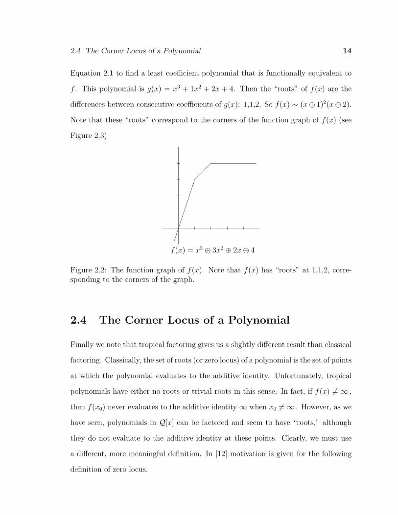
2.4 The Corner Locus of a Polynomial 14
Equation 2.1 to find a least coefficient polynomial that is functionally equivalent to
f . This polynomial is g(x) = x3 + 1x2 + 2x + 4. Then the “roots” of f(x) are the
differences between consecutive coefficients of g(x): 1,1,2. So f(x) ∼ (x⊕ 1)2(x⊕ 2).
Note that these “roots” correspond to the corners of the function graph of f(x) (see
Figure 2.3)
�����������
��
f(x) = x3 ⊕ 3x2 ⊕ 2x⊕ 4
Figure 2.2: The function graph of f(x). Note that f(x) has “roots” at 1,1,2, corre-sponding to the corners of the graph.
2.4 The Corner Locus of a Polynomial
Finally we note that tropical factoring gives us a slightly different result than classical
factoring. Classically, the set of roots (or zero locus) of a polynomial is the set of points
at which the polynomial evaluates to the additive identity. Unfortunately, tropical
polynomials have either no roots or trivial roots in this sense. In fact, if f(x) 6= ∞ ,
then f(x0) never evaluates to the additive identity ∞ when x0 6= ∞ . However, as we
have seen, polynomials in Q[x] can be factored and seem to have “roots,” although
they do not evaluate to the additive identity at these points. Clearly, we must use
a different, more meaningful definition. In [12] motivation is given for the following
definition of zero locus.

2.4 The Corner Locus of a Polynomial 15
Definition 4. Let f(x) ∈ Q[x]. The zero locus (or corner locus) Z(f) is defined to
be the set of points x0 in Q for which at least two monomials of f attain the minimum
value.
The di in (2.4) are precisely that points of Z(f), as we now show.
Theorem 6. Given a point d ∈ Q and a least-coefficient polynomial f(x) , x⊕ d is a
factor of f(x) if and only if f(d) attains its minimum on at least two monomials.
Proof. First, suppose that x ⊕ d is a factor of f(x) . If we write f as a product of
linear factors as in (2.4), di = d for some di .For all j < i ,
ai + i · di = ai + (i− j) · di + j · di
≤ ai + di + di−1 + · · ·+ dj+1︸ ︷︷ ︸i−j terms
+j · di
= aj + j · di .
A similar calculation shows that for j > i , we have ai + i · di ≤ aj + j · di . So
f(di) = aidii . Also, aid
ii = andndn−1 · · · di+1d
ii = andndn−1 · · · did
i−1i = ai−1d
i−1i , so
the minimum is attained by at least two monomials of f(x) at x = d .
For the other direction, suppose that the minimum is attained by two monomials
at f(d) . By way of contradiction, suppose that these monomials are not consecutive.
Then for some j < i < k , we have ajdj = akd
k < aidi . If x ≤ d then
ak + k · x = ak + i · x + (k − i) · x
≤ ak + i · x + (k − i) · d
= ak + k · d + i · (x− d)
< ai + i · d + i · (x− d)
= ai + i · x.
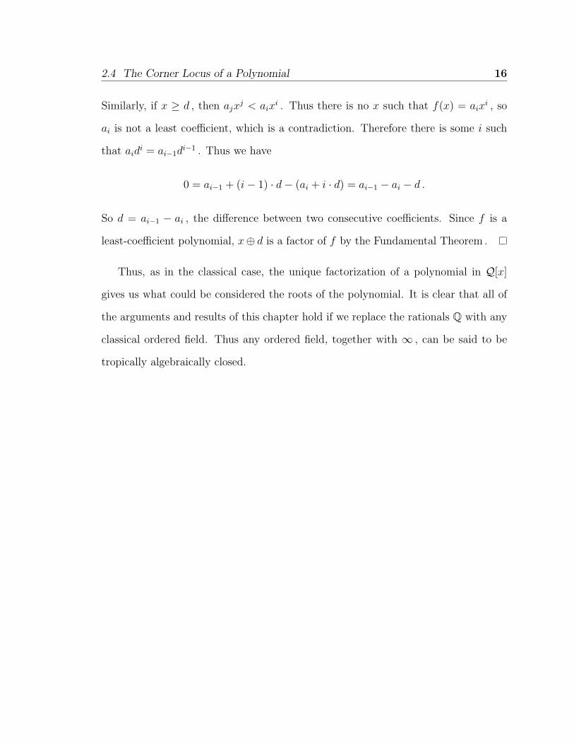
2.4 The Corner Locus of a Polynomial 16
Similarly, if x ≥ d , then ajxj < aix
i . Thus there is no x such that f(x) = aixi , so
ai is not a least coefficient, which is a contradiction. Therefore there is some i such
that aidi = ai−1d
i−1 . Thus we have
0 = ai−1 + (i− 1) · d− (ai + i · d) = ai−1 − ai − d .
So d = ai−1 − ai , the difference between two consecutive coefficients. Since f is a
least-coefficient polynomial, x⊕ d is a factor of f by the Fundamental Theorem .
Thus, as in the classical case, the unique factorization of a polynomial in Q[x]
gives us what could be considered the roots of the polynomial. It is clear that all of
the arguments and results of this chapter hold if we replace the rationals Q with any
classical ordered field. Thus any ordered field, together with ∞ , can be said to be
tropically algebraically closed.

Chapter 3
Tropical Polynomials of Several
Variables
Although we can factor every single-variable polynomial into linear factors, we have
no hope of being able to do the same for polynomials of two or more variables. In fact,
tropical polynomials in more than one variable do not always have unique factoriza-
tions.1 Nevertheless, the structure of the tropical zero locus makes it possible for us
to learn a lot more about tropical factorization than we would expect to be able to.
To make use of this structure, we discuss the tropical zero locus in detail. We discuss
polyhedral complexes and a correspondence between weighted balanced complexes
and tropical polynomials. We prove that factorization of tropical polynomials in two
or more variables is NP-complete. We then present a method in which we use the
structure of the tropical zero locus to find factorizations of polynomials.
Notation. In Chapter 2, we were very careful to distinguish between formal equality
and functional equivalence. In this chapter, we will not be so careful. We will now
consider two polynomials the same polynomial if they define the same function. In
1For example, the cubic polynomial x2y ⊕ xy2 ⊕ x2 ⊕ xy ⊕ y2 ⊕ x ⊕ y factors into irreduciblepolynomials as (x⊕ 0)(y ⊕ 0)(x⊕ y) or as (x⊕ y ⊕ 0)(xy ⊕ x⊕ y).
17

3.1 The Corner Locus and Weighted Balanced Complex 18
other words, we will write f = g to mean that f and g are functionally equivalent.
We will also use multi-index notation throughout this chapter. In other words,
we will write a polynomial f ∈ Q[x1, . . . , xn] as
f(x) =⊕I∈∆
aIxI ,
where I = (I1, . . . In) ∈ (Z+)n, and xi = x1I1x2
I2 · · ·xnIn . The set ∆ is called the
support of f . It is important to note that a tropical monomial aIxI is written classi-
cally as 〈x, I〉+aI , where 〈·, ·〉 is the scalar product and we think of x as (x1, . . . , xn).
Therefore, we have
f(x1, . . . , xn) = f(x) =⊕I∈∆
aIxI = min
I∈∆{〈x, I〉+ aI}.
It is also important to note that since our base field is Q = Q∪{∞}, our calcula-
tions will sometimes include multiplication by or subtraction of infinity. We will use
the convention that ∞ · 0 = 0 and ∞−∞ = 0.
3.1 The Corner Locus and Weighted
Balanced Complex
3.1.1 The Corner Locus
Definition 5. If f ∈ Q[x1, . . . , xn] is a polynomial then the tropical zero locus or
corner locus of f is the set
Z(f) := {α ∈ Qn : two or more monomials of f attain the minimum at α}.
Even though it is not technically a zero locus, we call Z(f) the tropical zero locus
because it is analogous to the classical zero locus. We often refer to Z(f) as the corner
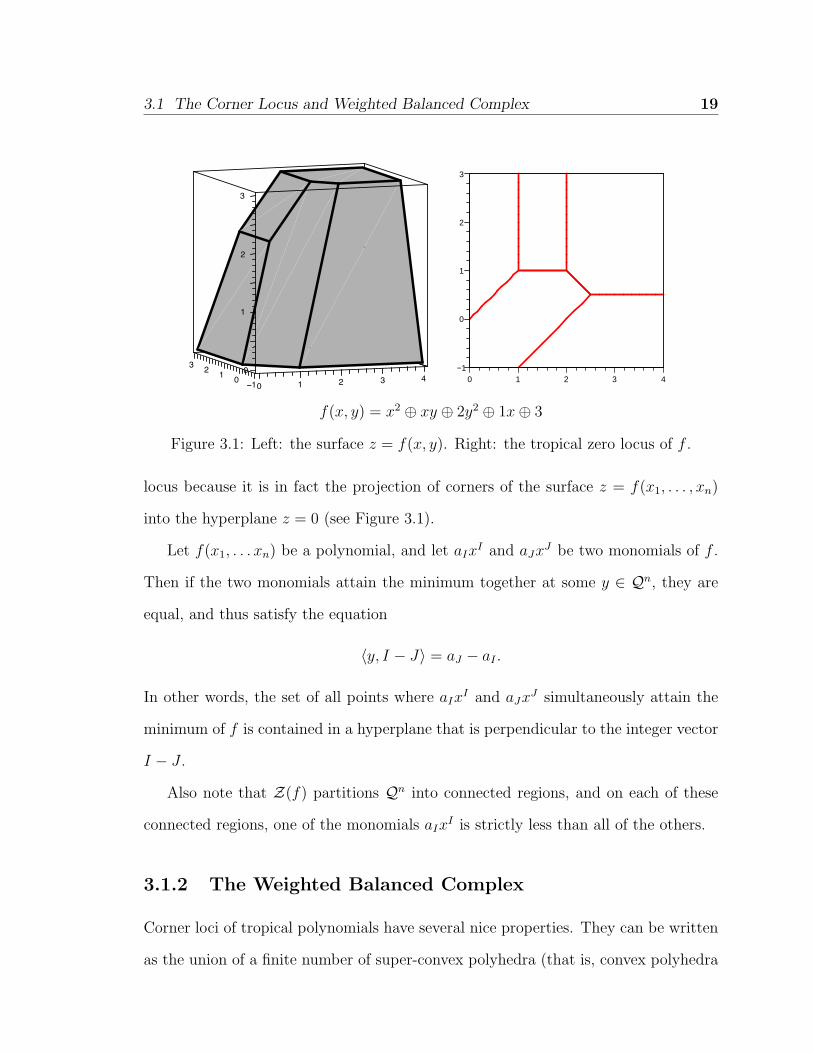
3.1 The Corner Locus and Weighted Balanced Complex 19
0
3 2 1−1
43210
0
1
2
3
−12 3 4
3
1
2
1
0
0
f(x, y) = x2 ⊕ xy ⊕ 2y2 ⊕ 1x⊕ 3
Figure 3.1: Left: the surface z = f(x, y). Right: the tropical zero locus of f .
locus because it is in fact the projection of corners of the surface z = f(x1, . . . , xn)
into the hyperplane z = 0 (see Figure 3.1).
Let f(x1, . . . xn) be a polynomial, and let aIxI and aJxJ be two monomials of f .
Then if the two monomials attain the minimum together at some y ∈ Qn, they are
equal, and thus satisfy the equation
〈y, I − J〉 = aJ − aI .
In other words, the set of all points where aIxI and aJxJ simultaneously attain the
minimum of f is contained in a hyperplane that is perpendicular to the integer vector
I − J .
Also note that Z(f) partitions Qn into connected regions, and on each of these
connected regions, one of the monomials aIxI is strictly less than all of the others.
3.1.2 The Weighted Balanced Complex
Corner loci of tropical polynomials have several nice properties. They can be written
as the union of a finite number of super-convex polyhedra (that is, convex polyhedra

3.1 The Corner Locus and Weighted Balanced Complex 20
whose faces of every dimension are also convex) that intersect each other only along
entire faces. The polyhedra can also be assigned weights and are balanced in a sense
that we will discuss later. We formalize all of this in the definition of a weighted
balanced complex. We also give the definition of a weighted balanced complex. Our
definitions are based on Mikhalikin’s definitions, given in [9].
Definition 6. A subset Π ⊂ Qn+1 is called a rational polyhedral complex (herein a
complex ) if it can be presented as a finite union of closed sets in Qn+1 called cells
with the following properties.
• Each cell is a closed convex (possibly semi-infinite or infinite) polyhedron. We
call a cell of dimension k a k-cell.
• Each cell has rational slope (i.e. its affine span is the kernel of a rational matrix).
• The boundary of a k-cell (that is, the boundary in the corresponding affine
span) is a union of (k − 1)-cells.
• Different open cells (that is, the interiors of the cells in the corresponding affine
spans) do not intersect.
For simplicity, we require all cells to be maximal in the sense that the union of two
distinct k-cells is not a k-cell. The dimension of a complex is the maximal dimension
of its cells. We call a complex of dimension n an n-complex.
Definition 7. A complex Π ⊂ Qn+1 is called weighted if there is a natural number
assigned to each n-cell of Π.
We are now ready to discuss what it means for a weighted complex to be balanced.
First, it is important to distinguish between boundary cells and interior cells.
3.1 The Corner Locus and Weighted Balanced Complex 21
Definition 8. In a complex Π ⊂ Qn+1, a boundary cell is a cell A that is contained
in a boundary hyperplane of Qn+1. In other words A ⊂ {(x1, . . . , xn) : xi = ∞} for
some i. An interior cell is a cell not contained in any boundary hyperplane.
Definition 9. In a complex Π ⊂ Qn+1, the integer covector of an interior n-cell F
is a vector c ∈ Zn such that c is normal to F , with the entries of c relatively prime.
Note an integer covector is only well-defined up to its sign. The covector becomes
well defined when we associate it with one of the regions of Qn+1 on either side of it.
The integer covector of an n-cell with respect to a region is the integer covector of
the n-cell that points from the n-cell into the region.
Definition 10 (Balancing Condition). Let Π ⊂ Qn+1 be a weighted n-complex with
the property that for k < n, every (k − 1)-cell is contained in the boundary of some
k-cell. Let r be an interior (n− 1)-cell of Π. Let {F1, . . . , Fk} be the set of n-cells in
Π containing r in their boundary. Then Π is balanced at r if for the weights ω1, . . . , ωk
corresponding to the Fi, we have
k∑i=1
ωici = 0,
where each ci is an integer covector corresponding to Fi and no two ci correspond to
the same region of the complement of Π.
We say that Π is balanced at the boundary if each boundary hyperplane either
contains no n-cells or is the union of a set of n-cells, all of which have the same
weight.
We say that Π is balanced (i.e. Π is a weighted balanced complex ) if Π is balanced
at each of its interior (n− 1)-cells and balanced at the boundary.
Note. Much work has been done regarding so-called tropical graphs and tropical
weighted balanced graphs that correspond to tropical curves (see [5, 13]). In Q2, a

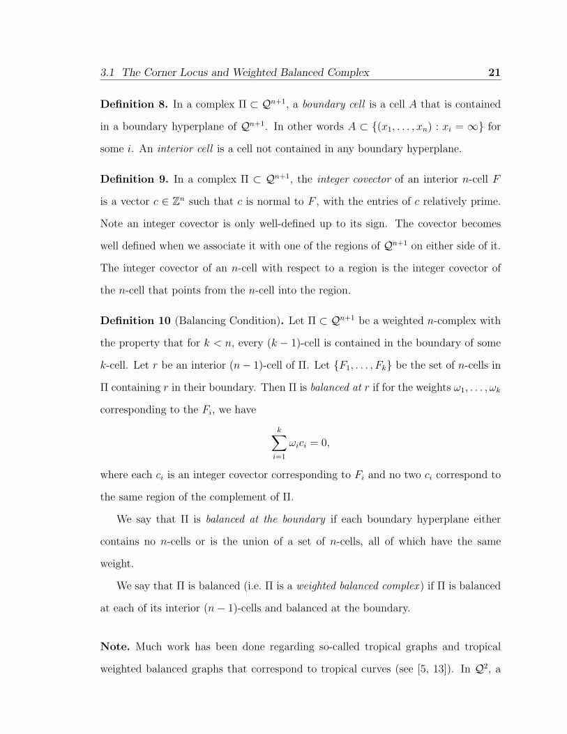
3.1 The Corner Locus and Weighted Balanced Complex 22
Figure 3.2: Corner locus of x⊕ y⊕ z⊕ 0: A weighted balanced 2-complex. Note that
the 2-cells are balanced around the 1-cells
weighted balanced 1-complex is a weighted balanced graph. The 1-cells of a weighted
balanced 1-complex correspond to the edges of a weighted balanced graph, and the
0-cells correspond to vertices. In this paper, we do not consider tropical graphs in Qn
for n > 2, since they do not correspond to the corner locus of a single polynomial.
For the same reason, we do not consider polyhedral complexes of codimension greater
than one.
Also, note that the balancing condition (together with our requirement that cells
of a complex be maximal) implies that each interior (n−1)-cell is in fact the boundary
of three or more n-cells.
3.1.3 Polynomial-Complex Correspondence
Theorem 7. There is a bijective correspondence between weighted balanced complexes
and tropical polynomials, up to functional equivalence and multiplication of the poly-
nomial by a scalar.

3.1 The Corner Locus and Weighted Balanced Complex 23
This theorem is proved by Mikhalkin in [9], although he does not use the language
of tropical polynomials. We should also note that Mikhalkin only proves the corre-
spondence up to multiplication by an indeterminant. It is easy to see that by using
Qn, we do not have this ambiguity. We also note that Mikhalkin proves the theorem
for Rn, while we only use Qn. Since Q is algebraically closed, Qn is sufficient.
Using this theorem, we can prove things about polynomials by proving things
about their corresponding weighted balanced complexes. For convenience, we will
give the correspondence explicitly.
The Weighted Balanced Complex Corresponding to a Polynomial. Let f
be a tropical polynomial. Mikhalkin has shown that Z(f) is a complex. We make
Z(f) into a weighted complex by assigning each n-cell F a weight as follows:
• If F a boundary n-cell, contained in the hyperplane corresponding to xi = ∞,
then xi divides f . Let m be the largest power of xi dividing f . The we assign
the weight m to F .
• If F is an interior n-cell, then F is the boundary between two (n+1)-dimensional
regions in Qn+1. If aIxI and aJxJ are the monomials corresponding to these
regions, then we define the weight of F to be the lattice length of the vector
I − J .2
Definition 11. The weighted balanced complex formed above is called the weighted
balanced complex of f and is denoted W(f).
The Polynomial Corresponding to a Weighted Balanced Graph Given a
weighted balanced complex Π ⊂ Qn+1, we construct a polynomial as follows.
2This weight is easily calculated to be the GCD of the entries of I − J .
3.2 Factors and Balanced Subcomplexes 24
1. Choose a region R0 of the complement of Π. Some monomial attains the mini-
mum on this region. Call it aIxI , where aI is arbitrary.
2. For every other region R of the complement of Π, choose a sequence of regions
R0, R1, . . . , Rk−1, Rk = R such that each Ri−1 is adjacent to the region Ri . For
1 ≤ i ≤ k, let Fi be the n-cell that separates Ri−1 from Ri. Let ωi be the weight
of Fi, and let ci be the integer covector corresponding to Fi and Ri. Assign the
monomial aJxJ to R, where
J = I −k∑
i=1
ωici .
3. Adjust the entries of I to be all positive, but as small as possible so that xim
divides f but xim+1 does not, where m is the weight of the n-cells in the xi
boundary, if there are any, and 0 otherwise.
4. Assign coefficients using the (n− 1)-cells.
3.2 Factors and Balanced Subcomplexes
Lemma 8. Let a, b, c, d ∈ Z2 with b − a and d − c multiples of the same primitive
integral vector e. Then the lattice length from a + c to b + d is the sum of the lattice
length from a to b and the lattice length from c to d.
Proof. Let b− a = ω1e and d− c = ω2e. Then ω1 and ω2 are the lattice lengths from
a to b and c to d respectively. It is clear that (b + d)− (a + c) = (b− a) + (d− c) =
ω1e + ω2e = (ω1 + ω2)e. So the lattice length from a + c to b + d is ω1 + ω2, as
desired.
Lemma 9 (Aaron Hill). If f and g are tropical polynomials, then the corner locus of
fg is equal to the union of the corner locus of f and the corner locus of g. In other
words, Z(fg) = Z(f) ∪ Z(g).

3.2 Factors and Balanced Subcomplexes 25
Proof. The proof is straightforward, and is given in [3].
Lemma 10. Let f, g ∈ Q[x1, . . . , xn+1], and let F be an n-cell of W(fg) ⊂ Qn+1.
Let ωf be the weight of the n-cell of W(f) that contains F , if such an n-cell exists,
or 0 if no such n-cell exists. Define ωg the same way. Then the weight of F is equal
to ωf + ωg.
Proof. If F is a boundary n-cell, then this follows directly from Definition 11. So we
may assume that F is an interior n-cell.
We will now prove that F is either contained in an n-cell of W(f) or the interior
of F is disjoint from W(f). Note that every point of a weighted balanced complex
is either in the interior of an n-cell or in the boundary of an n-cell. Small enough
neighborhoods of an interior point of an n-cell are contained in a hyperplane, while
neighborhoods of points on n-cell boundaries are not. Suppose that there is a point
α ∈ F ◦ ∩ W(f). Since α is in the interior of F , it must be in the interior of some
n-cell G of W(f). Let β be any other point of the interior of F . Since F is convex,
every point on the line segment from α to β is in the interior of F , and therefore not
in the boundary of G. So in fact, β must be in the interior of G, and we have F ⊂ G.
If F is contained in an n-cell of W(f), then there is one monomial of f for each
side of F that attains the minimum of f in that region. If the interior of F is disjoint
from W(f), then the same monomial attains the minimum on each side of F . The
same is of course true for W(g).
Let a and b correspond to the exponents of the monomials of f that attain the
minimum on either side of A, and let c and d correspond to the exponents of the
monomials of g that attain the minimum on either side of A (It is possible that c = d).
Now b− a = ωfe for some primitive integer vector e. It is clear that d− c = ωge for
the same vector e. So by Lemma 8, the weight of F is the lattice length from a + c

3.2 Factors and Balanced Subcomplexes 26
to b + d which is simply the lattice length from a to b plus the lattice length from c
to d, which is ωf + ωg, as desired.
1
1
1
1
11
11
1
2
2
3
f g fg
Figure 3.3: Weighted balanced graphs of f , g, and fg. Note that when a segmentoverlaps in the product, the weights add (see Lemma 10).
Definition 12. If G is a weighted complex, then a subset H of G is a subcomplex
of G if H is a complex, and each n-cell F of H has weight less than or equal to the
weight of the n-cell of G that contains F .
Lemma 11. If f is a factor of g then W(f) is a balanced subcomplex of W(g).
Proof. By definition, W(f) is a weighted balanced complex. Lemma 10 guarantees
that W(f) is a subcomplex of W(g).
Theorem 12. If G is a subcomplex of W(f) ⊂ Qn+1 that satisfies the balancing
condition, then the polynomial corresponding to G is a factor of f .
Proof. Consider W(f) as a collection of n-cells {F1, . . . , Fk}, with each Fi assigned a
weight ωi. We can think of G as the same collection of n-cells, with each Fi assigned
a weight σi, with 0 ≤ σi ≤ ωi. Note that we assign an n-cell Fi a weight of σi = 0 in
3.3 A Factoring Algorithm 27
G if Fi is not in G, otherwise σi corresponds to the weight of Fi in G. Also note that
while G may not be maximal in the sense that we required in Definition 6, this is of
little importance. Let H be the weighted complex given by {F1, . . . , Fk} with each
Fi assigned a weight ωi − σi.
We first prove that H satisfies the balancing condition. Let r be an interior (n−1)-
cell of H and let {Fn1 , . . . , Fnm} be the set of n-cells adjacent to r. Let {cn1 , . . . cnm}
be the integer covectors of the Fni, no two with respect to the same region of the
complement of H. Then we have
m∑i=1
(ωn1 − σni)cni
=m∑
i=1
ωnicni
−m∑
i=1
σnicni︸ ︷︷ ︸
both zero since W(f) and Gare respectively balanced
= 0− 0 = 0.
Thus, H is balanced at all of its interior (n − 1)-cells. It is clear that H is also
balanced at the boundary.
Let f1 be the polynomial corresponding to G and f2 the polynomial corresponding
to H. By Lemma 10, W(f1f2) = W(f). So in fact cf1f2 = f for some constant c.
Therefore, the polynomial f1 corresponding to G is a factor of f .
3.3 A Factoring Algorithm
3.3.1 NP-completeness
Theorem 13. The problem of factoring tropical polynomials in two or more variables
is NP-complete.3
3 NP stands for nondeterministic polynomial time, and we say that a problem is NP if it ispossible to verify a solution in polynomial time (though it may not be possible to find a solutionto such a problem in polynomial time). To say that factoring is NP-complete means that if wecould find factors in polynomial time (as opposed to just being able to verify them), then wecould solve every NP problem in polynomial time. In other words, this theorem asserts that it isextremely unlikely that a polynomial-time factoring algorithm exists. For more information, seehttp://mathworld.wolfram.com/NP-CompleteProblem.html

3.3 A Factoring Algorithm 28
Proof. It is clear that the problem of factoring tropical polynomials is NP, since the
weighted balanced complex of a polynomial can clearly be found in polynomial time,
and verifying that one polynomial is a factor of another is a matter of checking that
one weighted balanced complex is a subcomplex of the other.
In [4], Gao and Lauder show that the problem of decomposing Newton polyhedra
is NP-complete. We prove that any algorithm that would factor tropical polynomials
would decompose Newton polyhedra as well.
Let P be a two-dimensional Newton polyhedron, let v0 be a vertex of P and
for 1 ≤ i ≤ k, let ei be a primitive integer vector and ωi a weight such that for
1 ≤ j ≤ k, vk = v0 +∑j
i=1 ωiei. Since P is a polygon,∑k
i=1 ωiei = 0. So there is
a weighted balanced 1-complex with k edges (1-cells), each of which has weight ωi
and is perpendicular to ei. If we factor the polynomial corresponding to this complex
then we find a subcomplex, which corresponds to a summand of P by Lemma 13
of [4] (see Figure 3.4). Since decomposing Newton polyhedra is NP-complete, so is
factoring tropical polynomials.
Figure 3.4: If there were a polynomial-time algorithm to factor tropical polynomials,then the same algorithm would decompose Newton polyhedra. Since decompositionof Newton polyhedra is NP-complete, so is tropical factoring.
3.3.2 A factoring algorithm
Let f ∈ Q[x1, . . . xn+1] be a tropical polynomial. Let G = W(f) ⊂ Qn+1.
3.3 A Factoring Algorithm 29
1. Choose an n-cell F of G. Let S = {F}.
2. For each element Fi of S, analyze the (n − 1)-cells in the boundary of Fi to
determine if and how each (n− 1)-cell can be decomposed. If necessary, choose
one of the decompositions. Add all the n-cells of the decomposition to S.4
3. Repeat Step 2 until no new n-cells are added to S.
When the algorithm is finished, S will be a balanced subcomplex of G. So by
Theorem 12, the polynomial corresponding to S is a factor of f . It is possible,
however, that S = G, in which case we have found a trivial factor. Even if S 6= G,
there may be multiple (distinct) factorizations of f . It is necessary to repeat the
whole process, using all possible combinations of choices in Step 2 to determine all
possible factorizations of f or to determine that f is irreducible.
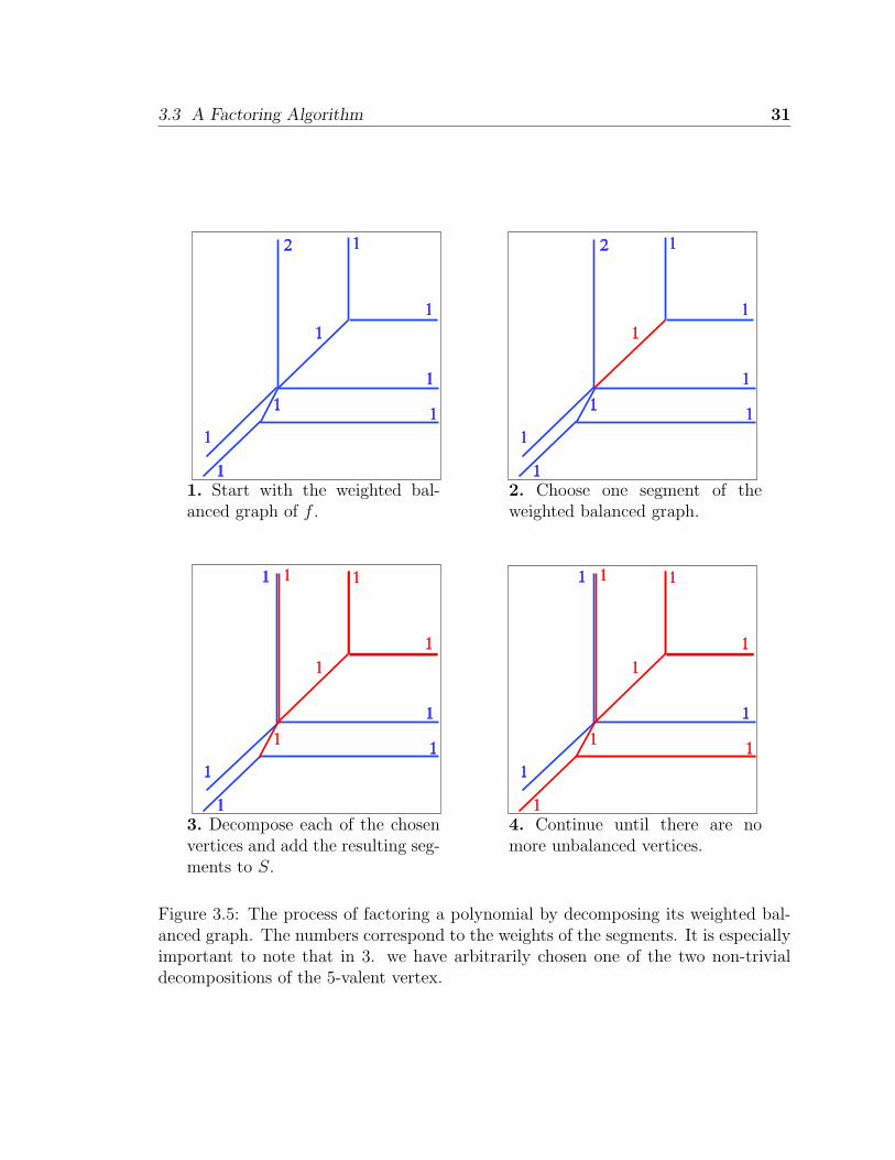
Example To see how the algorithm works, we will look at an example (see Fig-
ure 3.5). Let f = x3 ⊕ x2y ⊕ 1xy2 ⊕ 1y3 ⊕ x2 ⊕ xy ⊕ y2 ⊕ x ⊕ y ⊕ 2. The weighted
balanced graph G of f consists of 8 segments (1-cells) of weight 1 and one segment
of weight 2. There are two 3-valent vertices (0-cells) and one 5-valent vertex (shown
in part 1 of the figure).
We first choose one segment of G, as indicated in part 2 of the figure. By choosing
the segment, we have also chosen two vertices. We analyze each of these vertices to
decompose them. The upper right vertex cannot be decomposed, so we must add the
other two adjacent segments to our set. The lower left vertex can be decomposed, in
two different ways. We choose one of these decompositions and add the correspond-
ing segments to our set (shown in part 3). It is important to note that if we had
chosen the other decomposition, we would have gotten a different factorization, as
4Decomposing an (n−1)-cell is equivalent to decomposing a two-dimensional Newton polyhedron.For an algorithm that can do this, see [4].

3.3 A Factoring Algorithm 30
this polynomial can be factored in two different ways. Finally, this step has given us
one more vertex. It cannot be decomposed, so we add two more segments to our set
(part 4).
Since all of the vertices are now balanced, we have found a balanced subgraph,
which by Theorem 12 corresponds to a factor of f . This (red) balanced subgraph
corresponds to the polynomial x2 ⊕ 1y2 ⊕ x⊕ y ⊕ 2, while the remaining (blue) part
corresponds to the polynomial x⊕ y⊕ 0. The reader can check that these two factors
indeed multiply to give f .
3.3.3 Analysis
The efficiency of this algorithm depends on the number of decompositions of a the
(n−1)-cells ofW(f). For polynomials of a fixed degree, the number of decompositions
of the vertices of the corner loci of these polynomials is inversely proportional to the
number of vertices. So in general, for polynomials of a fixed degree, polynomials
whose corner loci have more vertices can be factored more efficiently.
One interesting attribute of this factoring algorithm is that regardless of the di-
mension of the polyhedral complex, the problem of decomposing (n − 1)-cells is the
same. Decomposing (n− 1) cells is equivalent to the problem of decomposing a two-
dimensional Newton polyhedron. In [4] it was shown that decomposing higher dimen-
sional Newton polyhedron can help factor classical polynomials. Since decomposing
an n-dimensional Newton polyhedron is equivalent to factoring a tropical polyno-
mial that has a single 1-cell, we can decompose an n-dimensional Newton polyhedron
simply by decomposing its two-dimensional faces.
3.3 A Factoring Algorithm 31
2 1
1
1
1
1
1
1
1
2 1
1
1
1
1
1
1
1
1. Start with the weighted bal-anced graph of f .
2. Choose one segment of theweighted balanced graph.
1 1
1
1
1
1
1
1
1
1 1 1
1
1
1
1
1
1
1
1
3. Decompose each of the chosenvertices and add the resulting seg-ments to S.
4. Continue until there are nomore unbalanced vertices.
Figure 3.5: The process of factoring a polynomial by decomposing its weighted bal-anced graph. The numbers correspond to the weights of the segments. It is especiallyimportant to note that in 3. we have arbitrarily chosen one of the two non-trivialdecompositions of the 5-valent vertex.

Chapter 4
Conclusion
I have shown that tropical polynomials with rational coefficients can be factored into
a product of linear polynomials. My elementary proof explains some of the nuances of
functional equivalence and introduces least-coefficient polynomials as representatives
of functional equivalences classes. I have given an algorithm to convert a polynomial
into least-coefficient form and show that least-coefficient polynomials can be factored
by inspection. Overall, my research provides a basis by which others can better
understand one-variable polynomials.
I have also shown that the problem of factoring tropical polynomials of two or
more variables is NP-complete. I have discussed weighted balanced complexes and
their usefulness in factoring tropical polynomials. I have also given an algorithm that
can factor tropical polynomials. My research on multi-variable polynomials provides
a better view at the geometry behind tropical polynomials.
I have also written some Maple programming code that can graph and manipulate
tropical polynomials. This code is included in Appendix 4, and has been very useful
to the BYU Tropical Algebra research group and will also be useful to others who
study tropical polynomials.
32

Appendix: The Tropical Maple
Package
During my research for this thesis and other related problems in tropical geometry, I
produced the Tropical Maple Package. It is compatible with Maple versions 10 and
higher. It is capable of graphing and otherwise manipulating tropical polynomials. It
can also compute tropical resultants and determinants of tropical matrices.
Perhaps the most useful of these procedures are plotgraph and graph, which
together with the internal procedure dual determine the corner locus of a polynomial
in two variables. Note that there is not an implementation of our factoring algorithm,
since this implementation was not completed at the time of printing.
Tropical:= module()
option package;
local trop,endpoints,Add,Multiply,Det,Isect,t,symcheck,
maxmin,cv,bestrange,LATEX,dual;
export Latex,tropical,coefs,graph,plotgraph,dualgraph,multiply,5
add,deriv,minfunc,plotgraphs,Poly,toLCP,isLCP,det,
SylvesterMatrix,resultant,makeparametric,makepoints,setCoordinates,
setMaxMin,maxfunc,colorlist,isect,toCCP;
maxmin:=-1; #change this to 1 for max or -1 for min
cv:=(a)->[a[1],a[2]];10
colorlist:=[red,green,blue,magenta,cyan,black,tan,yellow,navy,
coral,plum,grey,aquamarine];
trop:=proc(poly)
description "Convert a tropical polynomial into a list of classic15
33

Appendix: The Tropical Maple Package 34
polynomials. This allows the user to enter tropical polynomials in
standard polynomial form.";
if type(poly,‘+‘) then op(map(trop,[op(poly)]))
elif type(poly,‘*‘) then ‘+‘(op(map(trop,[op(poly)])))
elif type(poly,‘^‘) then ‘*‘(op(map(trop,[op(poly)])))20
elif type(poly,list(list)) then
seq(a[1]+a[2]*x+a[3]*y+‘if‘(nops(a)>3,a[4]*z,0), a in poly)
elif type(poly,Array) then
seq(poly[a,1]+poly[a,2]*x+poly[a,3]*y+‘if‘(op([2,2,2],poly)>3,
poly[a,4]*z,0),a=op([2,1],poly))25
elif type(poly,list(algebraic)) then op(poly)
else poly
fi;
end proc:
30
tropical:=poly->[eval(trop(poly),[‘0‘=0,‘1‘=1,zero=0,one=1,
‘-1‘=-1,minusone=-1])];
#The tropical function is what the user uses. It calls trop and then
makes certain substitutions to allow the user to enter polynomials
such as ‘1‘*x+‘0‘.35
minfunc:=proc(poly)
local s1,s2;
description "Returns a functional representation of a polynomial";
if nops([args])>1 then40
if type(op(2,[args]),symbol) then
s1:=convert(op(2,[args]),string)
else
s1:=convert(op(2,[args]),string)[2..-2]
fi;45
s2:=convert(min(op(tropical(poly))),string);
parse("("||s1|| ")->" ||s2);
else
min(op(tropical(poly)))
fi;50
end proc;
maxfunc:=proc(poly)
local s1,s2;
description "Returns a functional representation of a polynomial";55
if nops([args])>1 then
if type(op(2,[args]),symbol) then

Appendix: The Tropical Maple Package 35
s1:=convert(op(2,[args]),string)
else
s1:=convert(op(2,[args]),string)[2..-2]60
fi;
s2:=convert(max(op(tropical(poly))),string);
parse("("||s1|| ")->" ||s2);
else
max(op(tropical(poly)))65
fi;
end proc;
coefs:=proc(poly)
local f,g,clist,a,b,templist;70
description "Returns an array of the coefficients and powers of
polynomial terms for a polynomial in x,y,and z. Used internally,
but also useful to the user.";
clist:=[];
f:=tropical(poly);75
for g in f do
b:=[‘if‘(type(g,‘+‘),op(g),g)];
templist:=[0,0,0,0];
for a in b do
if member(’x’,indets(a)) then80
templist[2]:=a/x
elif member(’y’,indets(a)) then
templist[3]:=a/y
elif member(’z’,indets(a)) then
templist[4]:=a/z85
else templist[1]:=a
fi
od;
clist:=[op(clist),templist];
od;90
if nops([args])>1 then
clist
else
Array(1..nops(clist),1..4,clist);
fi;95
end proc:
graph:=proc(poly)
local duallines,lines,l1,l2,dir,p1,p2,p3,proj,t,opts,temp,s;
Appendix: The Tropical Maple Package 36
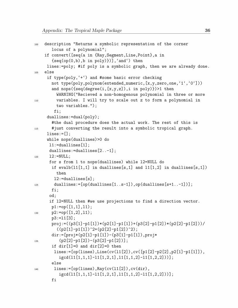
description "Returns a symbolic representation of the corner100
locus of a polynomial";
if convert([seq(a in {Ray,Segment,Line,Point},a in
{seq(op(0,b),b in poly)})],‘and‘) then
lines:=poly; #if poly is a symbolic graph, then we are already done.
else105
if type(poly,‘+‘) and #some basic error checking
not type(poly,polynom(extended_numeric,[x,y,zero,one,‘1‘,‘0‘]))
and nops({seq(degree(i,[x,y,z]),i in poly)})>1 then
WARNING("Recieved a non-homogenous polynomial in three or more
variables. I will try to scale out z to form a polynomial in110
two variables.");
fi;
duallines:=dual(poly);
#the dual procedure does the actual work. The rest of this is
#just converting the result into a symbolic tropical graph.115
lines:=[];
while nops(duallines)>0 do
l1:=duallines[1];
duallines:=duallines[2..-1];
l2:=NULL;120
for s from 1 to nops(duallines) while l2=NULL do
if evalb(l1[1,1] in duallines[s,1] and l1[1,2] in duallines[s,1])
then
l2:=duallines[s];
duallines:=[op(duallines[1..s-1]),op(duallines[s+1..-1])];125
fi;
od;
if l2=NULL then #we use projections to find a direction vector.
p1:=op([1,1],l1);
p2:=op([1,2],l1);130
p3:=l1[3];
proj:=((p3[1]-p1[1])*(p2[1]-p1[1])+(p3[2]-p1[2])*(p2[2]-p1[2]))/
((p2[1]-p1[1])^2+(p2[2]-p1[2])^2);
dir:=[proj*(p2[1]-p1[1])-(p3[1]-p1[1]),proj*
(p2[2]-p1[2])-(p3[2]-p1[2])];135
if dir[1]=0 and dir[2]=0 then
lines:=[op(lines),Line(cv(l1[2]),cv([p1[2]-p2[2],p2[1]-p1[1]]),
igcd(l1[1,1,1]-l1[1,2,1],l1[1,1,2]-l1[1,2,2]))];
else
lines:=[op(lines),Ray(cv(l1[2]),cv(dir),140
igcd(l1[1,1,1]-l1[1,2,1],l1[1,1,2]-l1[1,2,2]))];
fi
Appendix: The Tropical Maple Package 37
else #that is, if l2 is not NULL
lines:=[op(lines),Segment(cv(l1[2]),cv(l2[2]-l1[2]),
igcd(l1[1,1,1]-l1[1,2,1],l1[1,1,2]-l1[1,2,2]))];145
fi;
od;
fi;
opts:=[args[2..-1]];
temp:=’default’;150
hasoption(opts,type,’temp’,’opts’);
#return section
if temp=’parametric’ then
makeparametric(lines)
else155
lines;
fi;
end proc:
plotgraph:=proc(poly)160
local ff,gra,temp,opts;
description "Draws the tropical zero locus of a tropical polynomial";
#some basic error checking
if type(poly,list) and not (type(poly,list(list)) or
type(poly,list(anything))) then165
WARNING("First argument of plotgraph must be a single polynomial.
Use ’plotgraphs’ for multiple polynomials.");
elif not type(poly,polynom) and not type(poly,list(list)) and
not type(poly,list(anything)) then
WARNING("Unexpected first argument.");170
fi;
opts:=[args[2..-1]];
gra:=graph(poly);
#view
temp:=bestrange(gra);175
hasoption(opts,view,’temp’,’opts’);
opts:=[op(opts),view=temp];
#thickness
temp:=2;
hasoption(opts,thickness,’temp’,’opts’);180
if temp=’weights’ then
temp:=[seq(op(3,a),a in gra)];
fi;
opts:=[op(opts),thickness=temp];
#color185
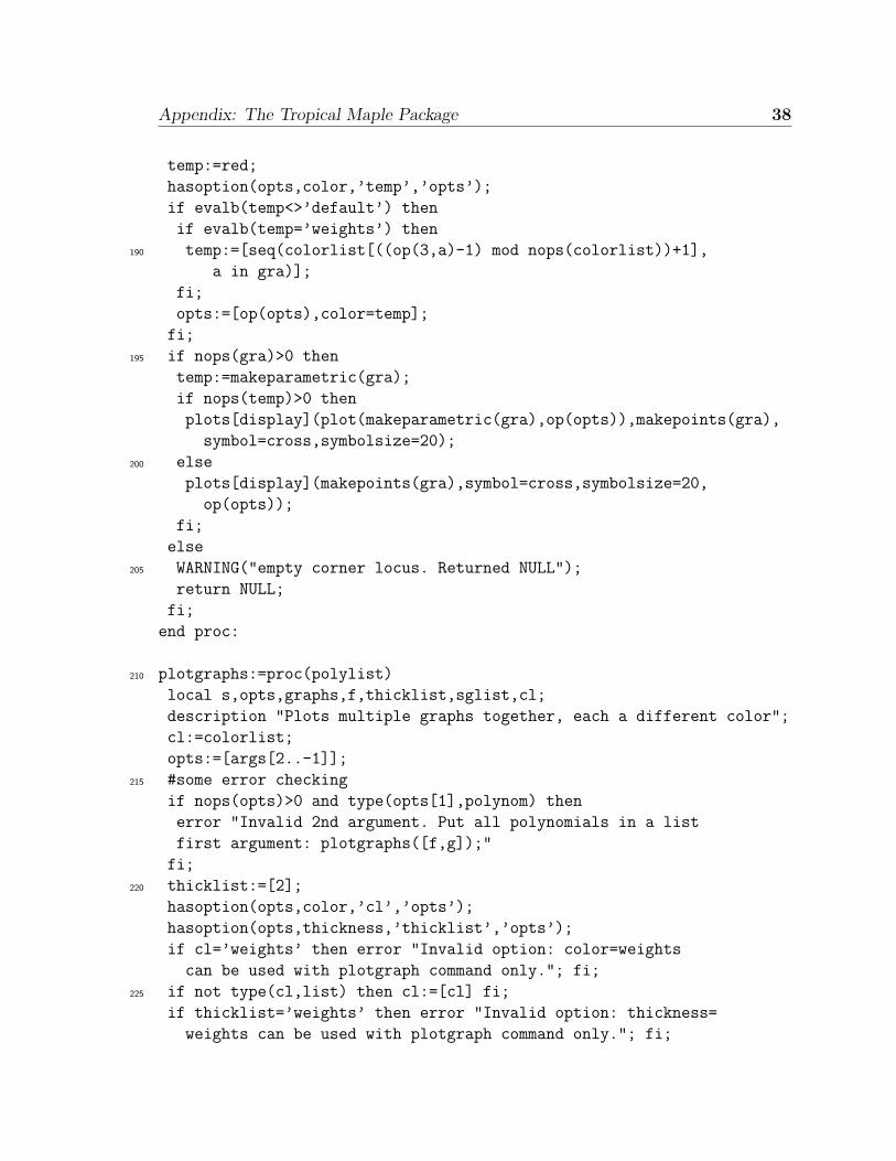
Appendix: The Tropical Maple Package 38
temp:=red;
hasoption(opts,color,’temp’,’opts’);
if evalb(temp<>’default’) then
if evalb(temp=’weights’) then
temp:=[seq(colorlist[((op(3,a)-1) mod nops(colorlist))+1],190
a in gra)];
fi;
opts:=[op(opts),color=temp];
fi;
if nops(gra)>0 then195
temp:=makeparametric(gra);
if nops(temp)>0 then
plots[display](plot(makeparametric(gra),op(opts)),makepoints(gra),
symbol=cross,symbolsize=20);
else200
plots[display](makepoints(gra),symbol=cross,symbolsize=20,
op(opts));
fi;
else
WARNING("empty corner locus. Returned NULL");205
return NULL;
fi;
end proc:
plotgraphs:=proc(polylist)210
local s,opts,graphs,f,thicklist,sglist,cl;
description "Plots multiple graphs together, each a different color";
cl:=colorlist;
opts:=[args[2..-1]];
#some error checking215
if nops(opts)>0 and type(opts[1],polynom) then
error "Invalid 2nd argument. Put all polynomials in a list
first argument: plotgraphs([f,g]);"
fi;
thicklist:=[2];220
hasoption(opts,color,’cl’,’opts’);
hasoption(opts,thickness,’thicklist’,’opts’);
if cl=’weights’ then error "Invalid option: color=weights
can be used with plotgraph command only."; fi;
if not type(cl,list) then cl:=[cl] fi;225
if thicklist=’weights’ then error "Invalid option: thickness=
weights can be used with plotgraph command only."; fi;

Appendix: The Tropical Maple Package 39
if not type(thicklist,list) then thicklist:=[thicklist] fi;
s:=0;
sglist:=map(graph,polylist); #make symbolic graphs230
if not(hasoption(opts,view)) then opts:=
[op(opts),view=bestrange([seq(op(o),o in sglist)])] fi;
graphs:=[];
for f in sglist do
graphs:=[op(graphs),plotgraph(f,op(opts),color=235
cl[(s mod nops(cl))+1],thickness=thicklist[(s mod
nops(thicklist))+1])];
s:=s+1;
od;
plots[display](graphs);240
end proc;
dual:=proc(poly)
local f,g,u,v,w,vertices,f0,fmin,t,points,h,hh,lines,xx,yy,det,
vertices2,ncc;245
description "Analyzes the dual of a polynomial in order to
draw the dual graph or the corner locus of a polynomial.";
f:=eval(tropical(poly),z=0);
g:=coefs(poly);
vertices:={}:250
vertices2:={};
ncc:={};
for u from 1 to nops(f) do
if u in ncc then next fi;
for v from u+1 to nops(f) do255
if v in ncc then next fi;
for w from v+1 to nops(f) do
if w in ncc then next fi;
det:=(g[u,2]-g[v,2])*(g[u,3]-g[w,3])-(g[u,2]-g[w,2])*
(g[u,3]-g[v,3]);260
if det<>0 then
xx:=(g[u,3]-g[w,3])/det*(g[v,1]-g[u,1])+(g[v,3]-g[u,3])/det*
(g[w,1]-g[u,1]);
yy:=(g[w,2]-g[u,2])/det*(g[v,1]-g[u,1])+(g[u,2]-g[v,2])/det*
(g[w,1]-g[u,1]);265
if not [xx,yy] in vertices2 then
f0:=eval(f,[x=xx,y=yy]);
fmin:=maxmin*max(op(maxmin*f0));
if fmin=f0[u] then
Appendix: The Tropical Maple Package 40
points:={};270
for t from 1 to nops(f0) do
if f0[t]=fmin then points:=points union {t} fi
od;
hh:=simplex[convexhull]([seq([maxmin*g[a,2],maxmin*g[a,3]],
a in points)]);275
vertices:=vertices union {[hh,[xx,yy]]};
vertices2:=vertices2 union {[xx,yy]};
for h in points do
if not [maxmin*g[h,2],maxmin*g[h,3]] in hh then
ncc:=ncc union {h}280
fi
od;
fi
fi
fi285
od
od
od;
lines:=[];
for v in vertices do290
hh:=v[1];
lines:=[op(lines),seq([{hh[t],hh[t+1]},v[2],hh[‘if‘(t+2>nops(hh),
t-1,t+2)]],t=1..nops(hh)-1),[{hh[1],hh[-1]},v[2],hh[2]]];
od;
if nops(lines)=0 then295
#this is in case there are no polygons in the dual (only edges)
vertices:={};
for u from 1 to nops(f) do
for v from u+1 to nops(f) do
if g[u,2]=g[v,2] then300
xx:=0;
yy:=(g[v,1]-g[u,1])/(g[u,3]-g[v,3]);
else
xx:=(g[v,1]-g[u,1])/(g[u,2]-g[v,2]);
yy:=0;305
fi;
f0:=eval(f,[x=xx,y=yy]);
fmin:=maxmin*max(op(maxmin*f0));
points:={};
for t from 1 to nops(f0) do310
if f0[t]=fmin then
Appendix: The Tropical Maple Package 41
points:=points union {maxmin*[g[t,2],g[t,3]]}
fi;
od;
if nops(points)>1 then315
vertices:=vertices union {[points,[xx,yy]]}
fi;
od
od;
lines:=[];320
for v in vertices do
hh:=[op(endpoints(v[1]))];
lines:=[op(lines),[{hh[1],hh[2]},v[2],hh[2]]];
od;
fi;325
lines;
end proc:
dualgraph:=proc(poly)
local d,g,pairedlines,lines,side,dotlist,pair;330
description "Graphs a tropical polynomial dual graph";
g:=coefs(poly);
pairedlines:=dual(poly);
if nops(pairedlines)=0 then
error "Empty corner locus"335
else
lines:={};
for pair in pairedlines do
lines:=lines union {pair[1]};
od;340
if member(’dots’,[args]) then
d:=degree(Poly(poly));
dotlist:=seq(seq(plottools[point]([maxmin*xx,maxmin*yy]),
xx=0..(d-yy)),yy=0..d);
else345
dotlist:=NULL
fi;
plots[display]([seq(plottools[line](op(1,l),op(2,l)),l in lines),
dotlist],tickmarks=[[-1="1"],[-1="1"]],axes=none,
scaling=constrained);350
fi;
end proc:

Appendix: The Tropical Maple Package 42
Multiply:=proc(poly)
local ff,p,f1,f2;355
description "Multiplies two or more polynomials
[internal for faster computing]";
if nargs=0 then return 0 fi;
ff:=Add(poly);
for p in args[2..-1] do360
ff:=Add([seq(seq(a+b,a in coefs(p,list)),b in coefs(ff,list))]);
od;
ff;
end proc;
365
multiply:=proc()
description "Multiplies two polynomials [for user]"
Poly(Multiply(args));
end proc;
370
Add:=proc(poly)
local t,ff,s,w;
description "Adds a number of polynomials";
w:=false;
ff:=[seq(op(coefs(p,list)),p in [args])];375
for t from 1 to nops(ff) while t<=nops(ff) do
if type(ff[t,1],infinity) then
#if ff[t,1]<>infinity then
#w:=true fi;
ff:=[op(ff[1..t-1]),op(ff[t+1..nops(ff)])];380
t:=t-1;
else
for s from t+1 to nops(ff) while s<=nops(ff) do
if ff[t,2]=ff[s,2] and ff[t,3]=ff[s,3] and ff[t,4]=ff[s,4] then
ff:=[op(ff[1..t-1]),[maxmin*max(maxmin*ff[t,1],maxmin*ff[s,1]),385
ff[t,2],ff[t,3],ff[t,4]],op(ff[t+1..s-1]),op(ff[s+1..nops(ff)])];
s:=s-1;
fi;
od;
fi;390
od;
#if w then WARNING("w") fi;
if nops(ff)=0 then
infinity
else395
ff

Appendix: The Tropical Maple Package 43
fi;
end proc;
add:=proc()400
Poly(Add(args));
end proc;
deriv:=proc(poly,vars)
description "Takes the derivative of a tropical polynomial";405
local d,a,var,dlist,onevar;
if type(vars,symbol) then onevar:=true else onevar:=false fi;
dlist:=[];
for var in vars do
d:=[];410
for a in tropical(poly) do
if member(cat(var),indets(a)) then d:=[op(d),a-var] fi;
od;
dlist:=[op(dlist),d]
od;415
if onevar then Poly(op(dlist)) else map(Poly,dlist) fi;
end proc;
endpoints:=proc(points)
local mx,Mx,my,My,p,ep;420
description "Finds the endpoints of a line segment [internal]";
mx:=min(seq(p[1],p in points));
Mx:=max(seq(p[1],p in points));
my:=min(seq(p[2],p in points));
My:=max(seq(p[2],p in points));425
ep:={};
for p in points do
if (p[1]>=Mx or p[1]<=mx) and (p[2]>=My or p[2]<=my) then
ep:=ep union {p}
fi430
od;
ep;
end proc;
Poly:=proc(poly)435
local g,t,c;
description "Makes a polynonmial out of a tropical polynomial";
if type(poly,polynom) then

Appendix: The Tropical Maple Package 44
poly
else440
g:=coefs(poly);
c:=op([2,1,2],g);
if c=0 then return infinity fi;
for t from 1 to c do
if g[t,1]=1 and (g[t,2]<>0 or g[t,3]<>0 or g[t,4]<>0) then445
g[t,1]:=‘1‘
elif g[t,1]=0 then
if g[t,2]=0 and g[t,3]=0 and g[t,4]=0 then
g[t,1]:=‘0‘
else450
g[t,1]:=1
fi;
fi;
od;
‘+‘(seq(g[t,1]*x^g[t,2]*y^g[t,3]*z^g[t,4],t=1..c));455
fi;
end proc;
isLCP:=proc(poly1)
local g,corners,u,v,tf,notinf,vertices,t,poly;460
description "Checks if a polynomial is least coefficients.";
tf:=true;
poly:=eval(poly1,z=‘0‘);
g:=coefs(poly);
notinf:=[seq([g[a,2],g[a,3]],a=op([2,1],g))];465
corners:=simplex[convexhull](notinf);
for u from min(seq(g[a,2],a=op([2,1],g))) to
max(seq(g[a,2],a=op([2,1],g))) while tf do
for v from min(seq(g[a,3],a=op([2,1],g))) to
max(seq(g[a,3],a=op([2,1],g))) while tf do470
if not evalb([u,v] in simplex[convexhull]([op(corners),[u,v]]))
and not evalb([u,v] in notinf) then
tf:=false
fi
od #v475
od; #u
if tf then
vertices:={seq(a[2],a in dual(poly))};
for t from 1 to op([2,1,2],g) while tf do
if g[t,1]>min(g[t,1],max(seq(eval(minfunc(poly),[x=v[1],y=v[2]])-480

Appendix: The Tropical Maple Package 45
g[t,2]*v[1]-g[t,3]*v[2],v in vertices))) then
tf:=false;
fi
od;
fi;485
tf;
end proc;
toLCP:=proc(poly1)
local g,corners,u,v,notinf,vertices,monomial,t,inf,s,poly;490
description "Determines a least coefficient polynomial
for a polynomial in two variables";
poly:=eval(poly1,z=‘0‘);
g:=coefs(poly);
notinf:=[seq([g[a,2],g[a,3]],a=op([2,1],g))];495
inf:=[];
corners:=simplex[convexhull](notinf);
for u from min(seq(g[a,2],a=op([2,1],g))) to max(seq(g[a,2],
a=op([2,1],g))) do
for v from min(seq(g[a,3],a=op([2,1],g))) to max(seq(g[a,3],500
a=op([2,1],g))) do
if not evalb([u,v] in simplex[convexhull]([op(corners),[u,v]])) and
not evalb([u,v] in notinf) then
inf:=[op(inf),[u,v,0]];
fi505
od #v
od; #u
s:=op([2,1,2],g);
g:=Array(1..s+nops(inf),1..4,g);
for t from 1 to nops(inf) do510
g[t+s,1]:=infinity;
g[t+s,2]:=inf[t,1];
g[t+s,3]:=inf[t,2];
g[t+s,4]:=inf[t,3];
od;515
vertices:={seq(a[2],a in dual(poly))};
for t from 1 to op([2,1,2],g) do
g[t,1]:=min(g[t,1],max(seq(eval(minfunc(poly),[x=v[1],y=v[2]])-
g[t,2]*v[1]-g[t,3]*v[2],v in vertices)));
od;520
Poly(g);
end proc;

Appendix: The Tropical Maple Package 46
toCCP:=proc(poly)
description "Converts a polynomial to Contributing Coefficient Form";525
local f,d,l,t;
d:=dual(poly);
l:={seq(op([maxmin*op([1,1],g),maxmin*op([1,2],g)]),g in d)};
f:=coefs(poly);
Poly([seq(‘if‘([f[t,2],f[t,3]] in l,f[t,1]+f[t,2]*x+f[t,3]*y+530
f[t,4]*z,NULL),t=op([2,1],f))]);
end proc;
Det:=proc(mat)
#errorchecking535
if type(mat,Matrix) then
if op([1,2],mat)<>op([1,1],mat) then
error "expected nxn matrix but received %1x%2 matrix",
op([1,1],mat),op([1,2],mat)
fi;540
if op([1,1],mat)=1 then
mat[1,1]
elif op([1,1],mat)=2 then
Add(Multiply(mat[1,1],mat[2,2]),Multiply(mat[1,2],mat[2,1]));
else #n>2545
Add(seq(Multiply(mat[1,i],Det(mat[2..op([1,1],mat),
[1..(i-1),(i+1)..op([1,1],mat)]])),i=1..op([1,1],mat)));
fi;
elif type(mat,list) and not type(mat,list(list)) then
if not type(sqrt(nops(mat)),integer) then550
error "list length must be the square of an integer.
(Received a list of length %1)",nops(mat);
fi;
Det(Matrix(sqrt(nops(mat)),sqrt(nops(mat)),[seq([seq(
mat[sqrt(nops(mat))*(i-1)+j],j=1..sqrt(nops(mat)))],555
i=1..sqrt(nops(mat)))]));
else
if not type(mat,list(list)) and not type(mat,array) then
WARNING("unrecognized input. Input should be of type
Matrix or list");560
fi;
Det(Matrix(mat));
fi;
end proc;
565
Appendix: The Tropical Maple Package 47
det:=proc()
Poly(Det(args));
end proc;
SylvesterMatrix:=proc(p1,p2,v)570
local M,t,s;
M:=LinearAlgebra[SylvesterMatrix](p1,p2,v);
for t from 1 to op([1,1],M) do
for s from 1 to op([1,2],M) do
if M[t,s]=0 then M[t,s]:=infinity fi;575
if M[t,s]=1 then M[t,s]:=0 fi;
od;
od;
M;
end proc;580
resultant:=proc(p1,p2,v)
det(SylvesterMatrix(p1,p2,v));
end proc;
585
makeparametric:=proc(o)
description "Returns a parametric version of a symbolic graph";
if nops([args])>1 then map(makeparametric,[args])
elif type(o,list) then map(makeparametric,o);
elif op(0,o)=’Line’ then590
[op([1,1],o)+op([2,1],o)*t,op([1,2],o)+op([2,2],o)*t,
t=-infinity..infinity]
elif op(0,o)=’Ray’ then
[op([1,1],o)+op([2,1],o)*t,op([1,2],o)+op([2,2],o)*t,t=0..infinity]
elif op(0,o)=’Segment’ then595
[op([1,1],o)+op([2,1],o)*t,op([1,2],o)+op([2,2],o)*t,t=0..1]
fi;
end proc:
makepoints:=proc(o)600
description "Returns a list of points extracted from a
symbolic graph";
if nops([args])>1 then map(makepoints,[args])
elif type(o,list) then map(makepoints,o);
elif op(0,o)=’Point’ then605
plottools[point](op(o));
fi;

Appendix: The Tropical Maple Package 48
end proc:
bestrange:=proc(symbolicgraph)610
description "Determines automatic range for a symbolic graph";
local r1,s;
r1:=[min(seq(op([1,1],g),g in symbolicgraph)),max(seq(op([1,1],g),
g in symbolicgraph)),min(seq(op([1,2],g),g in symbolicgraph)),
max(seq(op([1,2],g),g in symbolicgraph))];615
for s from 1 to 4 by 2 do
if r1[s]=r1[s+1] then
r1[s]:=r1[s]-1;
r1[s+1]:=r1[s+1]+1;
else620
r1[s]:=r1[s]-.5*(r1[s+1]-r1[s]);
r1[s+1]:=r1[s+1]+.5*(r1[s+1]-r1[s]);
fi
od;
s:=r1[2]-r1[1]-(r1[4]-r1[3]);625
if evalf(s)>0 then
r1[4]:=r1[4]+s/2;
r1[3]:=r1[3]-s/2;
else
r1[2]:=r1[2]-s/2;630
r1[1]:=r1[1]+s/2;
fi;
return [r1[1]..r1[2],r1[3]..r1[4]];
end proc;
635
Isect:=proc(object1,object2)
description "Internal procedure to determine intersection of two
Point-Segment-Ray-Line objects";
local oo,o1,o2,p,t,r;
o1:=symcheck(object1); o2:=symcheck(object2);640
if op(0,o1)=Point then
oo:=o1;o1:=o2;o2:=oo;
fi;
if op(0,o2)=Point then #o2 is a point
if op(0,o1)=Point then #if both are points645
if o1=o2 then return o1 else return NULL fi;
fi;
if op([2,2],o1)*(op([1,1],o1)-op([1,1],o2))<>op([2,1],o1)*
(op([1,2],o1)-op([1,2],o2)) then
return NULL;650

Appendix: The Tropical Maple Package 49
fi;
if op([2,1],o1)=0 then
t:=(op([1,2],o2)-op([1,2],o1))/op([2,2],o1)
else
t:=(op([1,1],o2)-op([1,1],o1))/op([2,1],o1)655
fi;
if op(0,o1)=Line or
(op(0,o1)=Ray and t>=0) or
(op(0,o1)=Segment and t>=0 and t<=1) then
return o2660
else
return NULL;
fi;
fi;
if op([2,1],o1)*op([2,2],o2)=op([2,2],o1)*op([2,1],o2) then665
#(they are parallel)
if op([2,2],o1)*(op([1,1],o1)-op([1,1],o2))<>op([2,1],o1)*
(op([1,2],o1)-op([1,2],o2)) then
return NULL;
fi;670
if op(0,o2)=Line then
oo:=o1; o1:=o2; o2:=oo;
fi;
if op(0,o1)=Line then #(one of them is a line)
return o2;675
fi;
if op(0,o1)=Ray and op(0,o2)=Ray then
if op([2,1],o2)*op([2,1],o1)+op([2,2],o2)*op([2,2],o1)>0 then
if (op([1,1],o1)-op([1,1],o2))*op([2,1],o1)+(op([1,2],o1)-
op([1,2],o2))*op([2,2],o1)>0 then680
return o1
else
return o2
fi;
else685
if (op([1,1],o2)-op([1,1],o1))*op([2,1],o1)+(op([1,2],o2)-
op([1,2],o2))*op([2,2],o2)>=0 then
return symcheck(Segment(op(1,o1),op(1,o2)-op(1,o1),
min(op(3,o1),op(3,o2))));
else690
return NULL;
fi;
fi;
Appendix: The Tropical Maple Package 50
fi; #(end case: both rays)
if op(0,o1)=Ray then695
oo:=o1; o1:=o2; o2:=oo;
fi;
if op([2,1],o1)=0 then
t:=[(op([1,2],o2)-op([1,2],o1))/op([2,2],o1),
op([2,2],o2)/op([2,2],o1)]700
else
t:=[(op([1,1],o2)-op([1,1],o1))/op([2,1],o1),
op([2,1],o2)/op([2,1],o1)]
fi;
if op(0,o2)=Ray then705
r:=[0,infinity]
else
r:=[0,1]
fi;
r:=sort([t[1],t[1]]+t[2]*r);710
r:=[max(0,r[1]),min(1,r[2])];
if r[2]>=r[1] then
return symcheck(Segment(op(1,o1)+op(2,o1)*r[1],op(2,o1)*
(r[2]-r[1]),min(op(3,o1),op(3,o2))));
else715
return NULL;
fi;
fi; #end case: they are parallel
#find the point where they would intersect
p:=[(op([2,2],o2)*(op([1,1],o1)-op([1,1],o2))-op([2,1],o2)*720
(op([1,2],o1)-op([1,2],o2)))/
(op([2,2],o1)*op([2,1],o2)-op([2,1],o1)*op([2,2],o2)),
(op([2,2],o1)*(op([1,1],o2)-op([1,1],o1))-op([2,1],o1)*
(op([1,2],o2)-op([1,2],o1)))/
(op([2,2],o2)*op([2,1],o1)-op([2,1],o2)*op([2,2],o1))];725
#(Cramer’s rule)
for t from 1 to 2 do
if op(0,[o1,o2][t])=Ray and p[t]<0 then
return NULL;
elif op(0,[o1,o2][t])=Segment and ((p[t])<0 or (p[t])>1) then730
return NULL;
fi;
od;
return Point(op(1,o1)+p[1]*op(2,o1));
end proc;735

Appendix: The Tropical Maple Package 51
isect:=proc(o1)
description "Returns the intersection of two symbolic graphs";
if o1=[] then return [] fi;
if type(o1,list({polynom,list})) then740
isect(op(o1));
elif nargs=1 then
graph(o1);
elif nargs=2 then
[op({seq(seq(Isect(a,b),a in graph(o1)),b in graph(args[2]))})];745
else
isect(isect(o1,args[2]),args[3..-1]);
fi;
end proc;
750
symcheck:=proc(object)
description "Checks a symbolic graph for validity";
if op(0,object)=Point and nops(object)<>1 then
error "Invalid Point Object";
fi;755
if op(0,object) in {Ray,Segment,Line} then
if nops(object)<>3 then
error "Invalid "||(op(0,object));
elif op(2,object)=[0,0] then
return Point(op(1,object))760
fi;
fi;
object;
end proc;
765
setCoordinates:=proc()
description "Sets the Coordinate System";
local c;
if nargs>1 then
error "expected one argument of type procedure or symbol,770
received %1 arguments",nargs
elif nargs=1 then
c:=op(1,[args]);
if type(c,procedure) then
cv:=c;775
elif type(c,symbol) then
if c=default then
cv:=a->[a[1],a[2]];

Appendix: The Tropical Maple Package 52
elif c=equilateral then
cv:=a->[a[1]-a[2]/2,sqrt(3)/2*a[2]];780
else
error "expected ’default’ or ’equilateral’ or user-defined
procedure,received ’%1’.",c;
fi;
else785
error "expected ’default’ or ’equilateral’ or user-defined
procedure,received type %1",whattype(c);
fi;
fi;
print(cv)790
end proc;
setMaxMin:=proc(x)
if x=’max’ then maxmin:=1; ’max’;
elif x=’min’ then maxmin:=-1; ’min’;795
fi;
end proc;
Latex:=proc(poly)
printf(LATEX(poly));800
end proc;
LATEX:=proc(poly);
if type(poly,‘+‘) then
cat("",seq(op([LATEX(op(i,poly))," \\oplus "]),i=1..805
(nops(poly)-1)),LATEX(op(-1,poly)));
elif type(poly,‘*‘) then
cat("",seq(LATEX(op(i,poly)),i=1..nops(poly)));
elif type(poly,‘^‘) then
cat("",LATEX(op(1,poly)),seq(op(["^{",op(i,poly),"}"]),810
i=2..nops(poly)));
elif type(poly,{numeric,symbol}) then
if type(poly,infinity) then
"\\infty "
else815
convert(poly,string)
fi;
elif type(poly,Matrix) then
cat(
"\\left[\\begin{array}{",seq("c",i=1..op([1,2],poly)),"}\n",820

Appendix: The Tropical Maple Package 53
seq(op([seq(op([LATEX(poly[i,j]),"&"]),j=1..op([1,2],poly)-1),
LATEX(poly[i,-1]),"\\\\\n"]),i=1..op([1,1],poly)-1),
seq(op([LATEX(poly[-1,j]),"&"]),j=1..op([1,2],poly)-1),
LATEX(poly[-1,-1]),
"\n\\end{array}\\right]");825
else
WARNING("I don’t know how do LaTeX that...I might have messed up.
(Type: %1)",whattype(poly));
convert(poly,string);
fi;830
end proc;
end module:
Bibliography
[1] Mike Develin, Tropical secant varieties of linear spaces, Discrete Comput. Geom.
35 (2006), no. 1, 117–129. MR MR2183492 (2006g:52024)
[2] Mike Develin and Bernd Sturmfels, Tropical convexity, Doc. Math. 9 (2004),
1–27 (electronic). MR MR2054977 (2005i:52010)
[3] Amanda Ellis, Classification of conics in the tropical projective plane, Master’s
thesis, Brigham Young University, December 2005.
[4] Shuhong Gao and Alan G. B. Lauder, Decomposition of polytopes and polynomi-
als., Discrete & Computational Geometry 26 (2001), no. 1, 89–104.
[5] Andreas Gathmann, Tropical algebraic geometry, Jahresber. Deutsch. Math.-
Verein. 108 (2006), no. 1, 3–32. MR MR2219706
[6] Andreas Gathmann and Hannah Markwig, The numbers of tropical plane curves
through points in general position, preprint http://arxiv.org/pdf/math.AG/
0504390, January 2006.
[7] Zur Izhakian, Tropical varieties, ideals and an algebraic nullstellensatz, preprint
http://arxiv.org/pdf/math.AC/0511059, 2005.
[8] G. L. Litvinov and V. P. Maslov (eds.), Idempotent mathematics and mathe-
matical physics, Contemporary Mathematics, vol. 377, American Mathematical
54
BIBLIOGRAPHY 55
Society, Providence, RI, 2005, Papers from the International Workshop held in
Vienna, February 3–10, 2003. MR MR2145152 (2006a:00008)
[9] Grigory Mikhalkin, Decomposition into pairs-of-pants for complex algebraic
hypersurfaces, Topology 43 (2004), no. 5, 1035–1065. MR MR2079993
(2005i:14055)
[10] , Tropical geometry and its applications, preprint http://arxiv.org/pdf/
math.AG/0601041, 2006.
[11] Lior Pachter and Bernd Sturmfels, Tropical geometry of statistical models,
Proc. Natl. Acad. Sci. USA 101 (2004), no. 46, 16132–16137 (electronic). MR
MR2114586
[12] Jurgen Richter-Gebert, Bernd Sturmfels, and Thorsten Theobald, First steps in
tropical geometry, Idempotent mathematics and mathematical physics, Contemp.
Math., vol. 377, Amer. Math. Soc., Providence, RI, 2005, pp. 289–317. MR
MR2149011 (2006d:14073)
[13] David Speyer, Tropical geometry, Ph.D. thesis, UC Berkeley, 2005.
[14] David Speyer and Bernd Sturmfels, Tropical mathematics, preprint http://arxiv.
org/pdf/math.CO/0408099, 2004.
Index
balancing condition, 23boundary cell, 23
cell, 22complex
rational polyhedral, 22weighted, 22weighted balanced, 21, 23
corner locus, 15, 20correspondence
polynomial-complex, 24
factorizationalgorithm, 30non-unique, 19, 31NP-completeness, 29
functional equivalence, 6, 20
graph,tropical, 24
integer covector, 23interior cell, 23
least coefficient, 7, 8least-coefficient polynomial, 8, 12
notation, 3, 20
Q, 3
Simon, Imre, 1subcomplex, 28
tropical algebraapplications , 1definition, 3fundamental theorem, 5, 13
tropical graph, 24
tropical zero locus, 15, 20
weighted balanced complex, 21of a polynomial, 25of a product, 27polynomial of, 25
weighted complex, 22
56


![Polynomial Statistics, Necklace Polynomials, and the ...tghyde/Hyde -- Thesis Defense.pdf · Factorization Statistics.Poly d(F q) = the set of monic degree d polynomials in F [x]..The](https://static.fdocuments.in/doc/165x107/5fab0ac0fcbc7304052f6b25/polynomial-statistics-necklace-polynomials-and-the-tghydehyde-thesis-defensepdf.jpg)

![3E28 Galois Theoryh008/teaching/3E28/3e28notes.pdf · Note also that factorization of polynomials in C[X] is (in theory) straightforward: the Fundamental Theorem of Algebra says that](https://static.fdocuments.in/doc/165x107/5f3b01ed4b8c5457c36b7941/3e28-galois-theory-h008teaching3e283e28notespdf-note-also-that-factorization.jpg)