![LOCALIZATION OF EILENBERG-MACLANE G-SPACES WITH …homology theories and ordinary homology and cohomology theories in § 1, following Wilson [16]. Given a homology theory h% and a](https://static.fdocuments.in/doc/165x107/5edc8695ad6a402d6667388f/localization-of-eilenberg-maclane-g-spaces-with-homology-theories-and-ordinary-homology.jpg)
FACTORIZATION HOMOLOGY Contents - NU Math Sitesnilay/pdf/... · homology is a machine that takes...
70
FACTORIZATION HOMOLOGY Contents 1. What is factorization homology? [09/20/17] 2 1.1. Introduction 2 1.2. Examples 2 2. How to come up with factorization homology yourself [09/22/17] 5 2.1. Kan extensions 5 2.2. Manifolds 6 3. Framings [09/25/17] 8 3.1. Framed embeddings, naively 8 3.2. Framed embeddings, homotopically 8 4. Homotopy pullbacks and framing [09/27/17] 11 4.1. Homotopy pullbacks 11 4.2. Framed vs rectilinear n-disks 12 5. Examples of n-disk algebras [09/29/2017] 14 6. Examples, continued [10/02/2017] 17 7. Homotopy colimits [10/04/2017] 19 8. Homotopy colimits, continued [10/06/2017] 21 8.1. Homotopy colimits 21 8.2. Factorization homology—a predefinition 21 9. ∞-categories [10/09/2017] 23 9.1. Topological enrichment 23 9.2. Complete Segal spaces and quasicategories 23 10. Colimits in ∞-categories [10/11/2017] 26 10.1. Colimits in 1-categories 26 10.2. Colimits in quasicategories 26 11. Homotopy invariance I [10/13/2017] 29 12. Homotopy invariance II [10/16/2017] 32 13. Homotopy invariance III [10/18/2017] 34 14. Back to topology [10/20/2017] 37 14.1. Finishing up homotopy invariance 37 14.2. Back to factorization homology 37 15. Computing factorization homology [10/25/17] 39 16. Nonabelian Poincar´ e duality I [10/27/2017] 41 17. Nonabelian Poincar´ e duality II [10/30/2017] 44 18. Nonabelian Poincar´ e duality III [11/01/2017] 46 19. Nonabelian Poincar´ e duality IV [11/03/2017] 48 20. Factorization homology is a homology theory [11/06/2017] 50 21. Nonabelian Poincar´ e duality VI [11/08] 52 22. Commutative algebras [11/10/2017] 54 23. Local systems and dualities [11/13/2017] 56 Date : Fall 2017. 1
Transcript of FACTORIZATION HOMOLOGY Contents - NU Math Sitesnilay/pdf/... · homology is a machine that takes...

FACTORIZATION HOMOLOGY
Contents
1. What is factorization homology? [09/20/17] 21.1. Introduction 21.2. Examples 22. How to come up with factorization homology yourself [09/22/17] 52.1. Kan extensions 52.2. Manifolds 63. Framings [09/25/17] 83.1. Framed embeddings, naively 83.2. Framed embeddings, homotopically 84. Homotopy pullbacks and framing [09/27/17] 114.1. Homotopy pullbacks 114.2. Framed vs rectilinear n-disks 125. Examples of n-disk algebras [09/29/2017] 146. Examples, continued [10/02/2017] 177. Homotopy colimits [10/04/2017] 198. Homotopy colimits, continued [10/06/2017] 218.1. Homotopy colimits 218.2. Factorization homology—a predefinition 219. ∞-categories [10/09/2017] 239.1. Topological enrichment 239.2. Complete Segal spaces and quasicategories 2310. Colimits in ∞-categories [10/11/2017] 2610.1. Colimits in 1-categories 2610.2. Colimits in quasicategories 2611. Homotopy invariance I [10/13/2017] 2912. Homotopy invariance II [10/16/2017] 3213. Homotopy invariance III [10/18/2017] 3414. Back to topology [10/20/2017] 3714.1. Finishing up homotopy invariance 3714.2. Back to factorization homology 3715. Computing factorization homology [10/25/17] 3916. Nonabelian Poincare duality I [10/27/2017] 4117. Nonabelian Poincare duality II [10/30/2017] 4418. Nonabelian Poincare duality III [11/01/2017] 4619. Nonabelian Poincare duality IV [11/03/2017] 4820. Factorization homology is a homology theory [11/06/2017] 5021. Nonabelian Poincare duality VI [11/08] 5222. Commutative algebras [11/10/2017] 5423. Local systems and dualities [11/13/2017] 56
Date: Fall 2017.
1

2 FACTORIZATION HOMOLOGY
23.1. Local systems 5623.2. Spooky duality 5724. Koszul duality [11/15/2017] 5925. The cotangent functor [11/20/2017] 6126. Koszul duality II [11/27/2017] 6326.1. Goodwillie calculus 6427. Manifold calculus [11/29/2017] 6627.1. Goodwillie-Weiss manifold calculus 66Appendix A. Exercises 69References 70
These are notes from John Francis’ “Factorization homology” course taught dur-ing the Fall quarter of the 2017 year at Northwestern. Errors and inaccuracies are,as usual, due to the notetaker(s).
1. What is factorization homology? [09/20/17]
1.1. Introduction. What is factorization homology? Well, if it were an animal, Icould describe it in two ways: distribution and phylogeny. More specifially, we willfirst see how factorization homology is distributed over the face of the planet. Thenwe will describe how it evolved from single-celled organisms, i.e. how you mightcome up with it yourself.
For the moment you can think of factorization homology as a sort of
generalized (co)sheaf homology.
Notice that this phrase can be hyphenated in two different ways. In one sense it isa generalization of the ideas of sheaf cohomology, and in the other it is a homologytheory for generalized sheaves (or sheaf-like objects). In particular, factorizationhomology is a machine that takes two inputs: a geometry M and an algebraicobject A. The output is ∫
M
A,
the factorization homology of with coefficients in A.
1.2. Examples. Let’s look at the first description: what are some examples offactorization homology that appear naturally in mathematics?
(1) Homology. Here M is a topological space and A is an abelian group. Inthis case the output is a chain complex∫
M
A ' H•(M,A),
quasiisomorphic to singular homology with coefficients in A.John: What is a theoremyou can’t prove without
ordinary homology? (2) Hochschild homology. Here M is a one-dimensional manifold – let’s takein particular M = S1 – and A will be an associative algebra. In this case∫
S1
A ' HH•A,
the Hochschild homology of A. You might be less familiar with this alge-braic object than ordinary homology. It’s importance comes from how

FACTORIZATION HOMOLOGY 3
it underlies trace methods in algebra (e.g. characteristic 0 representa-tions of finite groups). Hochschild homology is a recipient of “the uni-versal trace” and hence an important part of associative algebra. Notethat HH0A = A/[A,A].
(3) Conformal field theory. This is in some sense the real starting pointfor the ideas we will develop in this class. Here M is a smooth completeetc. algebraic curve over C and A is a vertex algebra. In this case theoutput
∫MA was constructed by Beilinson and Drinfeld, and is known as
chiral homology of M with coefficients in A. It is a chain complex, withH0(
∫MA) being the space of conformal blocks of the conformal field theory.
(4) Algebraic curves over Fq. Here M is an algebraic curve over Fq and Gis a connected algebraic group over Fq. In this case
∫MG is known as the
Beilinson-Drinfeld Grassmannian and is a stack. One interesting propertythat it has is that
H•
(∫M
G, Q`)' H•(BunG(M), Q`),
where here we are taking `-adic cohomology. Although the Beilinson-Drinfeld Grassmannian is more complicated than the stack of principalG-bundles, it is more easily manipulated. We note that the equivalenceabove is a form of nonabelian Poincare duality.
In particular, one might be interested in computing
χ(BunG(M)) =∑[P ]
1
|Aut(P )|,
which makes sense over a finite field. The computation of this quantity isknown as Weil’s conjecture on Tamagawa numbers.
(5) Topology of mapping spaces. Now M is an n-manifold without bound-ary andA will be an n-fold loop space, A = ΩnZ = Maps((Dn, ∂Dn), (Z, ∗)).The output is a space weakly homotopy equivalent to Mapsc(M,Z) ifπiZ = 0 for i < n. This is also known as nonabelian Poincare duality.Again the left hand side is more complicated but more easily manipulated.
(6) n-disk algebra (perturbative TQFT). Here M is an n-manifold and Ais an n-disk algebra (or an En-algebra) in chain complexes. The output is achain complex and has some sort of interpretation in physics. One thinks ofA as the algebra of observables on Rn, and
∫MA is the global observables
(in some derived sense). In a rough cartoon of physics, one assigns to openssets of observables, and a way to copmute expectation values. Factorizationhomology puts together local observables to global observables:
Obs(M) '∫M
A,
at least if we are working in perturbative QFT.(7) TQFT. Here M is an n-manifold (maybe with a framing) and A is an
(∞, n)-category (enriched in V). The output is a space (if enriched, an ob-ject of V), which is designed to remove the assumptions from the examplesabove.
That’s all the examples for now. Next class we’ll go over how one might havecome up with factorization homology. It is worth noting that in this class we will
4 FACTORIZATION HOMOLOGY
focus on learning factorization homology as a tool instead of aiming to reach somefancy theorem. Hopefully this will teach you how to apply it in contexts you mightbe interested in.
Pax: What is the physical interpretation of the first and second chiral homolo-gies? John: One might be interested in things like Wilson lines, where these higherhomology groups come into play.

FACTORIZATION HOMOLOGY 5
2. How to come up with factorization homology yourself [09/22/17]
2.1. Kan extensions. Consider the following thought experiment. Suppose youwant to study objects in some context M. Unfortunately objects here are prettyhard in general. Inside M, however, we have some objects D ⊂ M that areparticulary simple, and moreover we know that everything else in M is “built outof” objects in D.
Let’s consider the example where M is a nice category of (homotopy types of)topological spaces. Let D consist of the point, i.e. all contractible spaces. Now tostudy M we might map functors out of it into some category V. Let’s start withD instead. Consider Fun(∗,V). Of course this is canonically just V. How do weextend this to studying M? We have an obvious restriction map
Fun(M,V) Fun(∗,V).ev∗
We want to look for a left adjoint to this functor ev∗ John: If you don’t knowwhat a left adjoint is youshould learn it because Iwon’t tell you. No, I’m notjoking (laughs).
There are two different thingswe could do. We could ignore the homotopy-ness of everything, and take the naivecategorical left-adjoint. If, say V is the category of chain complexes, this naiveleft-adjoint produces a stupid answer. . . depending on what our precise definitionsare. Let’s suppose that by M we meant the homotopy category of spaces (hereobjects are spaces and maps are sets of homotopy classes of maps). Then we areextending
∗ V
hoSpaces
A
A naive left adjoint would take the functor A to the functor sending a space X to thestupid answer A⊕π0X (on morphisms take summands to summands correspondingto where the connected components are sent). Why is this a left adjoint?Similarly if we take M to be just
spaces and all continuous maps, X would be sent to A⊕X . Here by X we mean theunderlying set of elements of X.
There is a more sophisticated notion of a derived or homotopy left adjoint.Suppose now that by M we mean the topological category of spaces, where themapping sets are spaces equipped with the compact-open topology. Now we takea homotopy Kan extension. This fancy left adjoint will now send a space X tothe the chain complex C∗(X,A) (up to equivalence). Hence we see that we canrecover homology from this paradigm of extending a simpler invariant to the wholecategory.
How do we choose what D and M are? Suppose we want to study F(M) forM ∈ M. For concreteness, let’s say we’re studying manifolds. The most basicquestion to ask: is there a local-to-global principle for F? The simplest case is forF to be a sheaf, i.e.
F(M) limU∈U F(U).∼
If so you don’t need factorization homology, and you can just leave.For instance, consider F = C∗(Maps(·, Z)) taking spaces to chain complexes. Is
this a sheaf? Well if we forget about C∗, we get a sheaf, as a map into Z is thesame as giving maps on subsets of the domain that agree on overlaps. What does

6 FACTORIZATION HOMOLOGY
taking chains do? Well notice that
C∗(Maps(U∐
V,Z)) = C∗(Maps(U,Z)×Maps(V,Z))
= C∗(Map(U,Z))⊗ C∗(Maps(V,Z)).
This is not a sheaf because in this case tensor products and direct sums are neverthe same for these chain complexes!Why? So what can we do? We need to change whatwe consider D to be from open coverings to something else.
Idea: to study F maybe there are more general arrangements of D ⊂ M suchthat local-to-global principles still apply, without F being a sheaf.
2.2. Manifolds. The following problem will guide us for the next few weeks.
Let M be a manifold and let Z be a space. Calculate the homologyof the mapping space H•Maps(M,Z).
To begin, let us specify which categories we will be working with.
Definition 1. Let Mfldn be the (ordinary) category of smooth n-manifolds, withHom(M,N) = Emb(M,N) the set of smooth embeddings of M into N . Similarly,let Mfldn be the topological category of smooth n-manifolds, with Hom(M,N) =Emb(M,N) the space of smooth embeddings of M into N , equipped with thecompact open smooth topology.
The compact open smooth topology takes a bit of work to define, so we’ll leavethat as background reading. A good reference is Hirsch’s book on differential topol-ogy [Hir94]. Roughly, convergence in this topology is pointwise in the map as wellas all its derivatives. To get a feel for what this entails, consider a knot. Locallytighten the knot until the knot turns (locally) into a line. These knots would wouldconverge in the usual compact-open topology to another knot, but in the smoothtopology, they do not converge as the tightening procedure creates sharp kinks. Inparticular π0Emb(S1,R3) is very different from π0Embtop(S1,R3).
Definition 2. We define the category Diskn to be the full subcategory of Mfldnwhere the objects are finite disjoint unions of standard Euclidean spaces
∐I Rn.
Similarly the category Diskn is the full topological subcategory ofMfldn where theobjects are finite disjoint unions of Euclidean space.
Observe that HomDiskn(Rn,Rn) = Emb(Rn,Rn).
Lemma 3. The map Emb(Rn,Rn) → GLn(R) ' OnR given by differentiating atthe origin is a homotopy equivalence.
Proof sketch. There is an obvious map GLnR → Emb(Rn,Rn). One of the com-posites is thus clearly the identity. It remains to show that the other compositionis homotopic to the identity. The homotopy is given by shrinking the embeddingdown to zero.
This fact should fill you with hope. The objects which are building blocks of man-ifolds have automorphism spaces that are, up to homotopy, just finite-dimensionalmanifolds. Actually it will be useful to think of the n-disks as some sort of algebra.
Definition 4. An n-disk algebra in V is a symmetric monoidal functor A : Diskn →V.

FACTORIZATION HOMOLOGY 7
As we stated before, our first goal in this class is to understand the homologyH∗Maps(M,Z) using n-disk algebras and factorization homology.
Question from someone: what’s the relation with En-algebras? John: It turnsout that En-algebras are equivalent to n-disk algebras with framing.
Question from Tochi: what if you work with manifolds with boundary? John:well if you require boundaries to map to boundaries you can make the same defi-nitions. You then have to work with Euclidean spaces and half-spaces. You’ll endup with two types of algebras instead of just n-disk algebras.
8 FACTORIZATION HOMOLOGY
3. Framings [09/25/17]
3.1. Framed embeddings, naively.
Definition 5. A framing of an n-manifold M is an isomorphism of vector bundlesTM ∼= M × Rn.
Of course, not all manifolds have framings. For instance, one can check that all(compact oriented) two-manifolds except for S1 × S1 do not admit framings. Youmight use the Poincare-Hopf theorem, which expresses the Euler characteristic asa sum of the index of the zeroes of a vector field v on M that has isolated zeroes.Hence if M is framed, the Euler characteristic of M must be zero.
Here is an example of a theorem that John does not know how to prove withoutthe use of homology.
Theorem 6 (Whitney or Wu). Every orientable three-manifold admits a framing.
Pax: isn’t there a later proof of this via geometric methods by Kirby? John:well ok I don’t know how to prove it without homology. . .
Notice that any Lie group has a framing, as one takes a basis for the Lie alge-bra and pushes it forward by the group action. On the other hand, manifolds ofdimension four generally do not have framings (at least in John’s experience).
We can ask the following question: what is a framed open embedding? Thereare a few options. The naive (strict) option is as follows. Suppose that we havean open embedding M → N of framed manifolds. The pullback of TN is TM , wehave two different trivializations of TM . We might ask that the induced map oftrivial bundles M ×Rn →M ×Rn be the identity. In other words, we ask the twoframings to be the same.
Okay fine, but lets think about what we want the answer to be. Embeddings arevery flexible you can stretch them and twist them. But strict framed embeddings arevery rigid the way we’ve defined them above. For instance, they are automaticallyisometries (giving the fibers the usual Euclidean metric). But of course there aren’tvery many isometric embeddings into a compact manifold. Thus the strict definitionof a framed embedding is not what we want to work with.
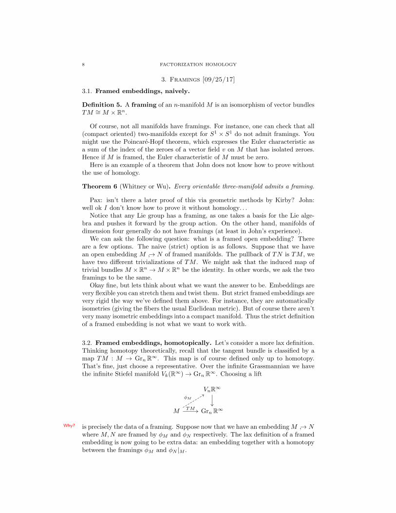
3.2. Framed embeddings, homotopically. Let’s consider a more lax definition.Thinking homotopy theoretically, recall that the tangent bundle is classified by amap TM : M → Grn R∞. This map is of course defined only up to homotopy.That’s fine, just choose a representative. Over the infinite Grassmannian we havethe infinite Stiefel manifold Vk(R∞)→ Grn R∞. Choosing a lift
VnR∞
M GrnR∞TM
φM
is precisely the data of a framing.Why? Suppose now that we have an embedding M → Nwhere M,N are framed by φM and φN respectively. The lax definition of a framedembedding is now going to be extra data: an embedding together with a homotopybetween the framings φM and φN |M .

FACTORIZATION HOMOLOGY 9
Definition 7. The space of framed embeddings Embfr(M,N) is the homotopypullback
Embfr(M,N) Emb(M,N)
MapsVnR∞(M,N) MapsGrn R∞(M,N)
In particular a framed embedding is an embedding M → N and a homotopy inMapGrn R∞(M,N) between the images along each map.
Exercise 8. Check that VnR∞ ' ∗.
With all this talk of homotopy pullbacks (which we’ll talk about in more detailnext time) it looks like we’ve made things more complicated, whereas we introduced
framings to make things simpler. Let’s calculate Embfr(Rn,Rn) as an example. Bydefinition, this sits in the following diagram
Embfr(Rn,Rn) Emb(Rn,Rn)
MapsVnR∞(Rn,Rn) MapsGrn R∞(Rn,Rn).
Notice that the bottom left object is homotopy equivalent to Maps∗(Rn,Rn) ' ∗.The bottom right space is homotopy equivalent to the loop space Ω Grn R∞ 'ΩBO(n) ' O(n). From last time, Emb(Rn,Rn) ' Diff(Rn) ' GL(n) ' O(n) (thisis homework 1). Now the vertical map on the right is a homotopy equivalence.This implies (by some machinery) that the vertical map on the left is an equivalence.We conclude that
Embfr(Rn,Rn) ' ∗.The rest of homework 1 is to show that Emb(Rn, N) is homotopy equivalent tothe frame bundle of TN . Applying this to the diagram above where we replace thesecond copy of Rn with N , we obtain
Embfr(Rn, N) Emb(Rn, N)
MapsVnR∞(Rn, N) MapsGrn R∞(Rn, N).
Now the same argument will show that the vertical map on the right is an equiva-lence, and that the map of the left is an equivalence. It follows now that
Embfr(Rn, N) ' N.
Hence we see that by adding framings we are replacing the role of the orthogonalgroup by that of a point. Indeed, this will allow for an easier transition betweenalgebra and topology.
Definition 9. We define the category D iskrectn to be the topological category con-
sisting of finite disjoint unions of open unit disks∐I D under rectilinear embed-
dings. In other words, embeddings which can be written as a composition of trans-lations and dilations. Here we use the usual topology indcued from the smoothcompact-open topology.

10 FACTORIZATION HOMOLOGY
One advantage of rectilinear embeddings is that they are easy to analyze. Forinstance, the space of embeddings from a single disk to a single disk is contractible:take an embedding, translate it to the origin, and the expand it outwards. In thisway D iskrect
n (D,D) = Embrect(D,D) deformation retracts onto the identity map.More generally, one checks that there is a homotopy equivalence
D iskrectn (
∐Dn, Dn) Confk(Dn)∼
Next time we will prove the following.
Proposition 10. There is a homotopy equivalence D iskrectn ' D iskfrn .

FACTORIZATION HOMOLOGY 11
4. Homotopy pullbacks and framing [09/27/17]
Let’s define more precisely some of the terms we used last time.
4.1. Homotopy pullbacks.
Definition 11. Suppose we have a map f : X → B together with a point ∗ ∈ B.The homotopy fiber of X → B over ∗ ∈ B is the fiber product
hofiber(f : X → B) := ∗ ×B Maps([0, 1], B)×B X.
In particular it is the space of triples (∗, φ, x) where φ(0) = ∗ and φ(1) = f(x).
hofiber(f) X
∗ B
Lemma 12. The formation of homotopy fibers is homotopy invariant. More pre-cisely, given an weak equivalence of spaces X → X ′ over B a pointed space viamaps f and g,
X X ′
B
then the homotopy fiber of f is weakly equivalent to the homotopy fiber of g.
Proof. Simply apply the (naturality of the) long exact sequence on homotopy groupsfor a Serre fibration to the map of fibrations Why are these fibrations?
hofiber(f) hofiber(g)
Maps([0, 1], B)×B X Maps([0, 1], B)×B X ′
B
We conclude that π∗ hofiber(f) ∼= π∗ hofiber(g).
Homework 2: Show, more generally, that homotopy pullbacks are homotopyinvariant.
Recall last time we were discussing MapsB(M,N) for some space B: maps “over”B. This object is defined to be the homotopy
MapsB(M,N) Maps(M,N)
∗ Maps(M,B)
In our case the map on the bottom is (a choice of) the map classifying the tangentbundle of M . Returning to last lecture, notice that by homotopy invariance wecan argue that MapsVnR∞(M,N) ' Maps(M,N) since VnR∞ ' ∗. Hopefully this
background fills in some of the gaps we left open during last lecture. But here we are usinghomotopy invariance in thebase?

12 FACTORIZATION HOMOLOGY
4.2. Framed vs rectilinear n-disks. Let us now return to our assertion from lasttime.What is a homotopy
equivalence of topologicalcategories?
Proposition 13. There is a functor D iskrectn → D iskfrn which is a homotopy equiv-alence.
Proof. Using the computations from last lecture we see that
D iskfrn(Rn,Rn) ' ∗ ' D iskrect
n (Dn, Dn).
What this functor does on objects is clear. On morphisms, the framing is deter-mined by the dilation factor present in the rectilinear embeddings. More generally,consider
D iskrectn
(∐I
Dn,∐J
Dn
)=
∐π:I→J
∏J
D iskrectn
∐π−1(j)
Dn, Dn
.
So it suffices to show that
D iskfrn
(∐I
Rn,Rn)' D iskrect
n
(∐I
Dn, Dn
).
Recall that ev0 : D iskrectn (
∐Dn, Dn) → ConfI(D
n) is a homotopy equivalence,which we mentioned ast time. Returning to our homotopy pullback square
Embrect(∐
Rn,Rn) Emb(∐
Rn,Rn)
∗ ' MapsEO(n)(∐
Rn,Rn) MapsBO(n)(∐
Rn,Rn)
notice that
Fr(TM) ' Emb(Rn,M) Emb((Rn, 0), (M,x)) ' O(n)
M x
ev0
Likewise
Emb(∐
Rn,M)∏I O(n)
ConfI(M) x1, . . . , xI
ev0
Hence MapsBO(n)(∐
Rn,Rn) '∏I MapsBO(n)(Rn,Rn) '
∏I O(n).
Up to homotopy, we now obtain
Embfr(∐
Rn,Rn) ConfI(Rn)×∏I O(n)
∗∏I O(n)
so we conclude that Embfr(∐
Rn,Rn) ' ConfI(Rn) which concludes the proof ofthe proposition.

FACTORIZATION HOMOLOGY 13
Example 14. Consider the case n = 1. What do the framed and rectilinearembeddings look like in this case? Well D iskfr
n(∐I R1,R1) ' ConfI(R1) is discrete
up to homotopy, and thus identified noncanonically with the symmetric group onI letters.
Recall a definition from the first day.
Definition 15. An En algebra in V is a symmetric monoidal functor D iskrectn → V⊗.
Next time we will see that E1-algebras are, in a suitable sense, equivalent toassociative algebras.

14 FACTORIZATION HOMOLOGY
5. Examples of n-disk algebras [09/29/2017]
Notice that we have a functor D iskfrn → D iskn. In particular, the former category
has less structure than the latter.Why is this?
Let’s recall the following way of thinking about a commutative algebra.
Definition 16. A commutative algebra in V⊗ (a symmetric monoidal category) isa symmetric monoidal functor
(Fin,∐
) (V,⊗),A
where Fin is the category of finite sets.
This probably looks a little unfamiliar, so let’s unpack it. Observe that theunderlying object is A = A(∗). The unit morphism is A(∅) = 1V → A(∗). Here1V is the symmetric monoidal unit in V. The multiplicative structure comes fromthe map from the two-point set to the one-point set, and the commutativity followsfrom the fact that this map is Σ2-invariant and that A is a symmetric monoidalfunctor so that A⊗2 → A is Σ2-invariant as well.
Definition 17. For V a symmetric monoidal topological category, an n-disk al-gebra is a symmetric monoidal functor D iskn → V. Similarly a framed n-diskalgebra is a symmetric monoidal functor D iskfr
n → V and a En-algebra is a sym-metric monoidal functor D iskrect
n → V.
Today we will discuss examples of n-disk algebras for V being chain complexesand toplogical spaces.
(1) There are the trivial n-disk algebras. For instance, consider A = Z, whichsends ∐
I Rn Z⊗I ∼= Z
and any embedding∐I Rn →
∐J Rn Z id−→ Z.
We can all agree that this is pretty trivial. More generally, we might takeA = Z⊕B, which sends
∐I Rn to (Z⊕B)⊗I and sends
∐I Rn → Rn to a
map (Z⊕B)⊗I → Z⊗B. What is this map? Let’s start by looking at thecase where |I| = 2. In that case take the map
Z⊕ Z⊗B ⊕B ⊗ Z⊕B ⊗B idZ⊕ idB ⊕ idB ⊕0−−−−−−−−−−−−→ Z⊕B.
You can generalize this for larger I – just take the product on the B factorsto be zero.This map looks weird. Fix it.
(2) Now let A : (Fin,∐
) → (Ch,⊗) be a commutative dg algebra. There isa natural symmetric monoidal functor π0 : (D iskn,
∐) → (Fin,
∐) which
sends∐I Rn 7→ π0(
∐I Rn) = I. The composition of these maps gives
us an n-disk algebra. The idea here is that in an n-disk algebra there isnot just one way of multiplying things. Indeed, there are Emb(
∐2 Rn,Rn)
multplications. What we have just done is used the π0 functor to reducethese various multiplications into the unique multiplication coming fromthe unique map from the two-point set to the one-point set.

FACTORIZATION HOMOLOGY 15
(3) The next example is that of an n-fold loop space of a pointed space (Z, ∗).We will construct a functor D iskn → Top and then postcompose with C∗to obtain a chain complex. This first functor is ΩnZ : D iskn → Top, whichwe will now define. Recall that for M a space and Z a pointed space, wesay that a map M → Z is compactly supported if there exists K ⊂ Mwith K compact and such that g|M\K = ∗ ∈ Z. Then we define
ΩnZ := Mapsc(−, Z) : (D iskn,∐
)→ (Top,×).
If you haven’t thought much about compactly supported maps then thereis something you have to check. Observe that if
U Z
V
g
the map U → V is an open embedding then the map g, given by sendinga point v to g(v) for v ∈ U and ∗ otherwise, is continuous (homework 3).Hence Mapsc is covariant via this extension by zero procedure. Moreoverit is symmetric monoidal as it sends disjoint unions to products.
Why is this called the n-fold loop space? Well notice that
ΩnZ = Maps((Dn, ∂Dn), (Z, ∗))' Mapsc(Rn, Z)
where we identify Rn with the interior of the closed disk Dn. In total, weget
D isknMapsc(−,Z)−−−−−−−−→ Top
C∗−−→ Ch
whose composite we write C∗ΩnZ. What happens if we don’t
use compactly supportedand take values in cochains?What is this n-disk algebrain terms of things we know?
(4) At the opposite end of the spectrum from trivial algebras are free algebras.The free En algebra on V ∈ (Ch,⊗), which we’ll notate as
FE(V ) : D iskrectn → Ch,
sends
Rn 7→⊕k≥0
C∗
(Embrect(
∐k
Dn, Dn)
)⊗Σk V
⊗k.
Here the Σk denotes the diagonal quotient. We will define what it does onmorphisms in a moment.
This has the universal property that given any map of chain complexesV → A for A an En-algebra (by this we mean a map of chain complexes V →A(Rn)), there exists a unique map of En-algebras such that the diagram
V A
FEn(V )
µ
commutes. The vertical map V → FEn is given by the inclusion into thek = 1 summand which is just V .

16 FACTORIZATION HOMOLOGY
What is this dashed map? For each k we need a map
C∗
(Embrect(
∐k
Dn, Dn)
)⊗Σk V
⊗k → A(Rn).
To do this we use the map
C∗
(Embrect(
∐k
Dn, Dn)
)⊗Σk V
⊗k µ⊗k−−→ C∗
(Embrect(
∐k
Dn, Dn)
)⊗Σk A
⊗k
and then use the multiplication for A. Let’s explain this. Notice that A :D iskrect
n → Ch and we have Embrect(∐kD
n, Dn)→ MapsCh(A⊗k(Dn), A(Dn))which by Dold-Kan (recall that everything is enriched in Top) correspondsto a map
C∗
(Embrect(
∐k
Dn, Dn)
)→ HomCh(A⊗k(Dn), A(Dn))
that is Σk-equivariant. Because of the equivariance it factors to the quo-tient, which gives us the multiplication map. Now apply (equivariant)tensor-hom adjunction to obtain this multiplication map. Okay, but wehaven’t yet shown that the free thing is actually an En-algebra, but we’reout of time.
(5) The last example we were gonna talk about is pretty awesome. Too badwe’re out of time.
Notice that if Z was an Eilenberg-MacLane space, there is overlap between ex-amples 2 and 3.

FACTORIZATION HOMOLOGY 17
6. Examples, continued [10/02/2017]
Last lecture we ran out of time in the proof of the following result.
Proposition 18. The functor FEn(V ) sending
Dn 7→⊕k>0
C∗
(Embrect(
∐k
Dn, Dn)
)⊗Σk V
⊗k
is the free En-algebra on V ∈ Ch.
Proof. Last time we showed that this functor satisfied the correct universal propertythough we hadn’t yet specified what it did on morphisms. To define what it doesto morphisms we need to construct a map
Embrect(∐I
Dn, Dn)→ MapsCh(FEn(V )⊗I ,FEn(V )).
By the Dold-Kan correspondence this is equivalent to specifying a map
C∗(Embrect(∐I
Dn, Dn))→ Hom(FEn(V )⊗I ,FEn(V ))
which by the tensor-(internal)hom adjunction, is equivalent to the data of a map
C∗(Embrect(∐I
Dn, Dn))⊗FEn → FEn(V ),
in other words, a map
C∗(Embrect(∐I
Dn, Dn))⊗
⊕k>0
C∗(Emb(∐k
Dn, Dn))⊗Σk V⊗k
⊗I → FEn(V ).
Let’s maybe just look at the left hand side in the case where I ∼= 0, 1:
C∗(Embrect(∐2
Dn, Dn)⊗⊕k0,k1
(C∗(Embrect(
∐k0
Dn, Dn))⊗Σk0V ⊗k0 ⊗ C∗(Embrect(
∐k1
Dn, Dn))⊗Σk1V ⊗k1
)
=⊕
k0,k1≥0
C∗
(Embrect(
∐2
Dn, Dn)× Embrect(∐k0
Dn, Dn)× Embrect(∐k1
Dn, Dn)
)⊗Σk0
×Σk1V ⊗(k0+k1)
But from this last expression it is easy to see now that we have a map from what’sin the parentheses to Embrect(
∐k0+k1
Dn, Dn)⊗Σk0+k1V ⊗(k0+k1) by composing the
embeddings (up to keeping track of the symmetric group).
Let’s talk about the example that we didn’t have time to discuss at the end oflast class. This is the class of En enveloping algebras of Lie algebras. Let g be aLie algebra. For simplicity we’ll work over R. John: this works for Lie
algebras valued in spectratoo, up to some changes.We define a functor D iskn → AlgLie(ChR) which sends U 7→ Ω∗c(U, g), i.e. a
Euclidean space to its space of compactly supported de Rham forms. Notice thatthis construction sends disjoint unions to direct sums. We now postcompose withthe Chevalley complex CLie
∗ (or if you like CLie∗ (g) ' R ⊗L
Ug R). We will write this
composite functor as CLie∗ (Ω∗c(•, g)), and it sends disjoint unions to tensor products.
D iskn AlgLie(ChR) ChR

18 FACTORIZATION HOMOLOGY
We will use the fact that
CLie∗ (g⊕ g′) ' CLie
∗ (g)⊕ CLie∗ (g′).
We claim that for n = 1,CLie∗ (Ω∗c(R1, g)) ' Ug.
In particular this functor which maps Lie algebras to En-algebras is left-adjoint tothe forgetful functor AlgEn → AlgLie.
Here’s a small aside. Where is this Lie algebra structure coming from? Wellnotice that we have a map
C∗(Embrect(∐2
Dn, Dn))⊗A⊗2 → A.
But notice that the left-hand side is homotopic to C∗(Sn−1) (do this exercise!). At
the level of homology, this gives a map H∗ Sn−1 ⊗R (H∗A)⊗2 → H∗A. There are
two generators for the homology of Sn−1 and so we a degree 0 map
H∗A⊗H∗A→ H∗A,
which is the associative algebra structure. However, we have another map comingfrom the fundamental class of Sn−1,
(H∗A⊗H∗A)[n− 1]→ H∗A,
is a Lie algebra structure on H∗A[1−n]. (Everything here should be valued in Ch)A reference for this forgetful functor is a paper by F. Cohen.
Since we’re almost out of time, let me give you a hint of what we’ll be doingnext. In factorization homology we are given some functor A : D iskn → Ch (or intoTop). Factorization homology is an extension∫
M
A = hocolim (D iskn/MA−→ Ch)
an extension that fits into
D iskn/M Ch
Mfldn
A
We need to define not only the homotopy colimit but also what we mean byD iskn/M . What do we want it to be? Its mapping spaces should fit into thehomotopy pullback diagram
MapsD iskn/M(U, V ) Emb(U, V )
∗ Emb(U,M)
V →M
U→M
As usual, if we require this to be a pullback instead of a homotopy pullback thisspace will be too small. In fact, it will be empty. Okay, you say – so let’s just definea category of n-disks with these mapping spaces. The problem that you will runinto here is that the composition will be associative only up to homotopy due to thecomposition of the paths in Emb(U,M) required by the adjective “homotopy”. Sowe’ll have to dip our toes into the theory of infinity-categories, which neatly dealswith both this issues and homotopy colimits.
FACTORIZATION HOMOLOGY 19
7. Homotopy colimits [10/04/2017]
We are interested in proving the following result.
Theorem 19. The homotopy colimit is homotopy invariant. More precisely, giventwo functors F,G : C → Top and any natural transformation α : F =⇒ G suchthat for all c ∈ C, α(c) : F (c)→ G(c) is a homotopy equivalence, then
hocolimC F ' hocolimC G
is a homotopy equivalence.
Notice that we can replace homotopy equivalence everywhere with weak homo-topy equivalence. Actually we will sketch the proof. The details will be left ashomework 4. There is a problem in the usual theory of colimits: they are nothomotopy invariant. Consider the following simple example. We have a map ofspans
Dn Sn−1 Dn
∗ Sn−1 ∗where the vertical arrows are homotopy equivalences. But the colimits of the topand bottom rows are Sn and ∗ respectively, which are of course not homotopyequivalent.
We have two basic tools that we will use to fix this: Mayer-Vietoris and Seifert-van Kampen.
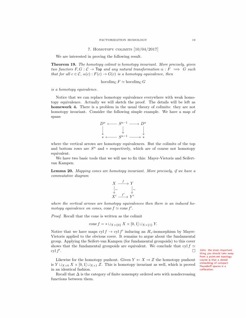
Lemma 20. Mapping cones are homotopy invariant. More precisely, if we have acommutative diagram
X Y
X ′ Y ′
f
∼ ∼
f ′
where the vertical arrows are homotopy equivalences then there is an induced ho-motopy equivalence on cones, cone f ' cone f ′.
Proof. Recall that the cone is written as the colimit
cone f = ∗ tX×0 X × [0, 1] tX×1 Y.
Notice that we have maps cyl f → cyl f ′ inducing an H∗-isomorphism by Mayer-Vietoris applied to the obvious cover. It remains to argue about the fundamentalgroup. Applying the Seifert-van Kampen (for fundamental groupoids) to this covershows that the fundamental groupoids are equivalent. We conclude that cyl f 'cyl f ′. John: the most important
thing you should take awayfrom a point-set topologycourse is that a closedembedding of compactHausdorff spaces is acofibration.
Likewise for the homotopy pushout. Given Y ←− X −→ Z the homotopy pushoutis Y tX×0 X × [0, 1] tX×1 Z. This is homotopy invariant as well, which is provedin an identical fashion.
Recall that ∆ is the category of finite nonempty ordered sets with nondecreasingfunctions between them.

20 FACTORIZATION HOMOLOGY
Definition 21. A simplicial space is a functor X• : ∆op → Top. The geometricrealization |X•| is the colimit
|X•|∐n≥0Xn ×∆n
∐[m]→[l]Xl ×∆m
The basic principle is that the “generators” are given by coproducts and the“relations” are given by reflexive coequalizers. For homotopy colimits the gener-ators will still be coproducts, but the relations will be handled by the geometricrealization.
Definition 22. For X• a simplicial space, the nth latching object LnX• is
(1) LnX• = colim(∆op
<n)/[n]
Xm ⊂ Xn
The index category is the category of maps [n]→ [m] for m < n.Think of this as all thedegenerate simplices induced
from everything below n. We say that X is Reedy cofibrant if the map LnX• → Xn is a cofibration forall n.
Lemma 23. If we have a map of simplicial spaces X• → Y• such that both X andY are Reedy cofibrant with the induced maps Xn ' Yn homotopy equivalences then|X•| ' |Y•|.
Proof outline. We proceed by induction on skeleta. In particular we have the geo-metric realization of the n-skeleton
| sknX•|∐k6nXk ×∆k
∐[m]→[l];m,l6nXl ×∆m
These skeleta sit inside the total geometric realization as closed embeddings whence|X•| = lim | sknX•|. So we will prove |X•| ' |Y•| by proving that | sknX•| '| skn Y•. The base case just says that sk0X•X0 ' Y0 = sk0 Y0. For the inductivestep check that there is a pushout
LnX ×∆n∐LnX×∂∆n Xn × ∂∆n skn−1X•|
Xn ×∆n sknX•|
Likewise for Y . By the inductive hypothesis we know that the map from the topright of the diagram for X to the top right of the diagram for Y is a homotopyequivalence. By assumption the same is true for the bottom left corner. Similarlyone has to prove that the top left is a homotopy equivalence. It is then importantthat the top and left arrows are cofibrations to conclude that the n-skeleton of Xis homotopy equivalent to the n-skeleton of Y .
Write out the details of this proof as homework 4.Let’s now turn to homotopy colimits. Given C a category we have a simplicial
object NC∗ : ∆op → Set, the nerve of C. Observe that the ordinary colimit alwaysreceives a surjective map from the coproduct of the functor applied to all the objectsin the indexing category. In particular the colimit will always be this coproductquotiented by a relation coming from morphisms in C. For homotopy colimits wewill get a map F : NC → Top sending [p] 7→ tNCpF and hocolimC F = |F•|.

FACTORIZATION HOMOLOGY 21
8. Homotopy colimits, continued [10/06/2017]
8.1. Homotopy colimits. Recall that if we have an ordinary functor F : C → Topthen the colimit colimC F can be expressed as a coequalizer: a quotient of thecoproduct of F (c) for all c ∈ C by the maps in C (every colimit is a reflexivecoequalizer of coproducts).
Definition 24. Given F : C → Top we write F• : ∆op → Top for the functor send-ing [n] 7→
∐NCn F (c0) (where c0 is the first object in the simplex). The simplicial
structure maps are given by copmosition and identities as usual. Then we definethe Bousfield-Kan homotopy colimit
hocolimC F := |F•|
Notice that every homotopy colimit is a geometric realization of coproducts.
Theorem 25 (Homotopy invariance of hocolim). Suppose we have two functorsF,G : C → Top such that F (c) and G(c) are cofibrant (i.e. CW complexes) forall c ∈ C, and there is a natural transformation α such that α(c) is a homotopyequivalence. Then hocolimC F ' hocolimC G.
Proof. This is homework 4 (from last time). Recall that the lemma from last timetells us that given a map of Reedy cofibrant simplicial spaces X• → Y• inducingequivalences on n-simplices for every n, the geometric realizations are equivalent.Hence we need only check Reedy cofibrancy for F• and G•.
In this case the nth latching object of F• is
LnF• =∐
F (c0)
where the coproduct is taken over all degenerate n-simplices of NC. But by the CWcomplex assumption above the maps LnF• → F• is a cofibration, as desired.
8.2. Factorization homology—a predefinition.
Definition 26. We define Diskn/M to be the category of n-disks embedding in Mwith morphisms given by inclusion (it is equivalent to the subposet of opens on Msuch that the image is diffeomorphic to an n-disk).
We can make the following predefinition (easier to make, harder to work with).Given A : Diskn → Top we define the factorization homology∫
M
A := hocolimDiskn/M A.
Really we should be working with the topological version D iskn/M but it will endup being homotopy equivalent.
We want factorization homology∫MA to be M , where we replace Rn with A(Rn).
Example 27 (Desiderata).
(1) if A = ∗? Then we would like∫M∗ ' ∗.
(2) if A(∐I Rn) =
∐I Rn then
∫M
id 'M.
(3) be able to compute∫MA for A belonging to the examples we discussed
earlier. For instance, commutative algebras, n-fold loop spaces, free n-diskalgebras, trivial n-disk algebras, and enveloping algebra of a Lie algebra.
(4) if A lands in Ch sending∐I Rn 7→ A⊕I then
∫MA ' C∗(M,A) (and likewise
for spectra).
22 FACTORIZATION HOMOLOGY
We need tools for computing homotopy colimits. For instance, it is useful tointroduce the topological version,
Diskn/M → D iskn/M ,
and it turns out that homotopy colimits over these two categories are equivalent.To make statements like this, we need crieria for when two homotopy colimits areequivalent when they’re indexed by different categories.
Since we don’t have time left today to introduce∞-categories, let’s go over someproperties of hocolim.
Theorem 28 (Quillen’s theorem A). Let g : C → D is a functor. If F is somefunctor from D to some target (such as topological spaces). Then
hocolimC F ' hocolimD F
if and only if g is final. In other words, for d ∈ D, define Cd/ := C ×D Dd/, andsay that g is final if B(Cd/) ' ∗ where BC := hocolim ∗.
There is another key property of homotopy colimits involving hypercovers. Sup-pose we have a functor C → Opens(X) → Top. When is
hocolimC F ' X?
Define, for x ∈ X, Cx to be the full subcategory of objects c such that x ∈ F (c). IfBCx ' ∗ for each x ∈ X then hocolimC F ' X.
Exercise 29. hocolim∗ F = F (∗).

FACTORIZATION HOMOLOGY 23
9. ∞-categories [10/09/2017]
9.1. Topological enrichment. Suppose we have a category T with products aswell as a functor ∆→ T from the ordinal category. Then MapsT (s, t) is a simplicialset with
MapsT (s, t)p = HomT (s× [p], t),
where by [p] we denote the image of the functor. If we now apply geometric real-ization, we obtain mapping spaces.
Consider for example T = Top (as a non-enriched, ordinary category). Thereis a functor ∆ → Top which sends [p] to the geometric p-simplex. Then we get asimplicial set MapsTop(X,Y )•, and notice that
MapsTop(X ×∆p, Y ) ∼= MapsTop(∆p,MapsTop(X,Y ))
where we equip the set MapsTop(X,Y ) with the compact-open topology, as usual.Hence the simplicial set MapsTop(X,Y )• is isomorphic to the singular simplicial setSing MapsTop(X,Y ). If we apply the geometric realization, since |SingA| ' A, wesee that we obtain the usual topological enrichment (at least up to homotopy) onthe category Top.
This trick allows us to enrich various categories in Top. As we have seen abovethe category of topological spaces is an immediate example, and it is not hard todo similarly for the category of simplicial sets. Another two familiar examples arethose of chain complexes and natural transformations of functors. For a slightlyunfamiliar example one could use the functor ∆ → CAlgop
R of de Rham forms onsimplices, which sends [p] 7→ Ω∗(∆p), to give the (opposite) category of commuta-tive R-algebras a topological enrichment.
This leads us to the following general idea, which highlights the importance oftopological enrichment.
Principle: Everywhere where there is a notion of homotopy, thereexists an enrichment in Top such that this is an actual homotopy.
9.2. Complete Segal spaces and quasicategories. Now, whatever∞-categoriesare, they should have two properties:
(1) The collection of ∞-categories up to some notion of equivalence should beequal to the collection of topological categories modulo homotopy equiva-lence (see below for the formal definition).
(2) Colimits, limits, functor categories, over/undercategories in ∞-categoriesare homotopy colimits, homotopy limits, etc. in the corresponding topo-logical category.
Definition 30. Let F : C → D be a functor between topological categories. Wesay that F is a homotopy equivalence if for each c, c′ ∈ C, MapsC(c, c
′) 'MapsD(Fc, Fc′) and every object d ∈ D is homotopy equivalent to some F (c) forc ∈ C. In other words, there exists a map d → Fc such that MapsD(e, d) →Maps(e, Fc) is a homotopy equivalence for all e ∈ D.
So that’s roughly the philosophy of∞-categories. They are a nice ground to workon when dealing with homotopy invariance. When it comes to actually defining∞-categories, there is a conceptual option and a more economical option: completeSegal spaces and quasicategories, respectively. Let me tell you briefly about com-plete Segal spaces.
24 FACTORIZATION HOMOLOGY
When we are given C a category, there is a set of objects and a set of morphisms.However, the only way we ever use categories is up to equivalence, and these un-derlying sets have no invariance properties with respect to equivalence of categories(for instance the sets of objects or corresponding sets of morphisms need not havethe same number of elements). This leads us to the question: how can we think ofa category in a way that better reflects the homotopy theory (i.e. equivalences) ofcategories.
It turns out that we can construct spaces of objects and morphisms of C in thefollowing way. Consider the underlying groupoid C0 ⊂ C where we have thrownout all the noninvertible maps. Taking the nerve (classifying space) NC0 gives usa simplicial set. The associated space is of course the geometric realization |NC0|.For morphisms, consider the category Funiso([1], C) of functors [1]→ C with naturaltransformations through isomorphisms. This category is a also a groupoid, so weobtain a space |N Funiso([1], C)|.
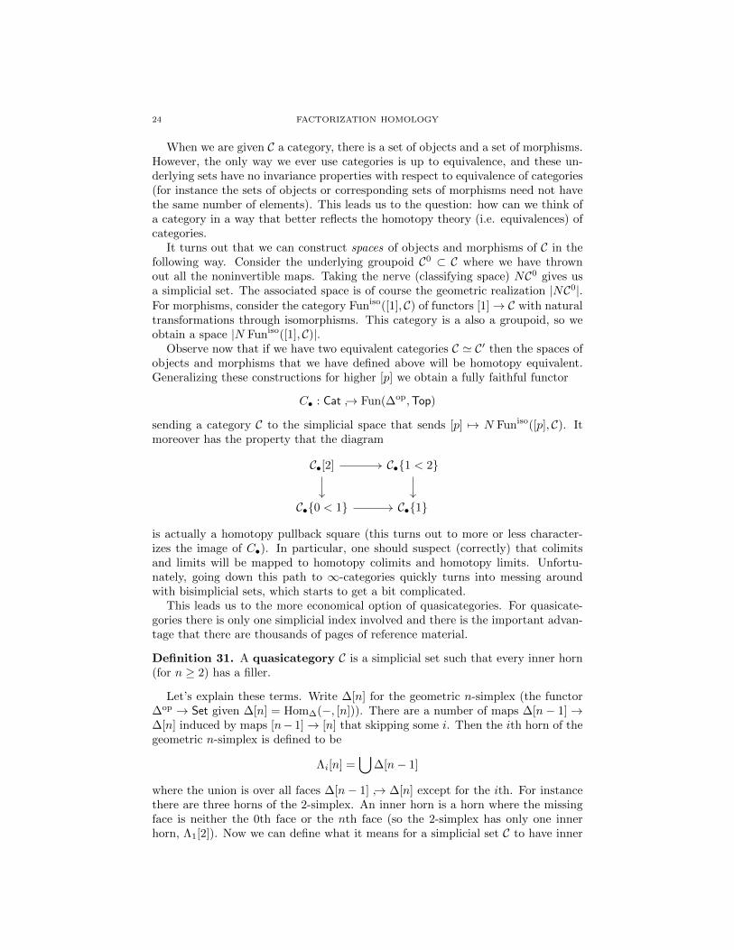
Observe now that if we have two equivalent categories C ' C′ then the spaces ofobjects and morphisms that we have defined above will be homotopy equivalent.Generalizing these constructions for higher [p] we obtain a fully faithful functor
C• : Cat → Fun(∆op,Top)
sending a category C to the simplicial space that sends [p] 7→ N Funiso([p], C). Itmoreover has the property that the diagram
C•[2] C•1 < 2
C•0 < 1 C•1
is actually a homotopy pullback square (this turns out to more or less character-izes the image of C•). In particular, one should suspect (correctly) that colimitsand limits will be mapped to homotopy colimits and homotopy limits. Unfortu-nately, going down this path to ∞-categories quickly turns into messing aroundwith bisimplicial sets, which starts to get a bit complicated.
This leads us to the more economical option of quasicategories. For quasicate-gories there is only one simplicial index involved and there is the important advan-tage that there are thousands of pages of reference material.
Definition 31. A quasicategory C is a simplicial set such that every inner horn(for n ≥ 2) has a filler.
Let’s explain these terms. Write ∆[n] for the geometric n-simplex (the functor∆op → Set given ∆[n] = Hom∆(−, [n])). There are a number of maps ∆[n− 1]→∆[n] induced by maps [n− 1]→ [n] that skipping some i. Then the ith horn of thegeometric n-simplex is defined to be
Λi[n] =⋃
∆[n− 1]
where the union is over all faces ∆[n− 1] → ∆[n] except for the ith. For instancethere are three horns of the 2-simplex. An inner horn is a horn where the missingface is neither the 0th face or the nth face (so the 2-simplex has only one innerhorn, Λ1[2]). Now we can define what it means for a simplicial set C to have inner

FACTORIZATION HOMOLOGY 25
horn fillings. It means that for every map Λi[n]→ C there is a lift, or “filling”,
Λi[n] C
∆[n]
of the map to the simplex making the diagram commute.
Example 32. Spaces and categories are two natural sources of quasicategories.
(1) Consider C = Sing(X). By the adjunction between geometric realizationand Sing the data of a map Λi[n] → SingX is precisely the data of amap |Λi[n]| → X. Now one can choose (there is no unique choice) saya retraction |∆[n]| → |Λi[n]|. Composing with the map to X and againapplying adjointness, we obtain a map ∆[n]→ SingX making the relevantdiagram commute. We conclude that the singular simplicial set of a spaceis a quasicategory.
(2) Given a category C consider the nerve C = NC. By the Yoneda lemma amap Λ1[2]→ NC is precisely the data of a composable pair of morphismsin C. In particular there is a unique way of filling the horn into the simplexby using the composition of these two maps. A similar argument holds forhigher-dimensional horns. We conclude that the nerve of any category is aquasicategory.
What we will do next is give the definitions of colimits, limits, functor categories,and over/undercategories in quasicategories. We will also discuss a variant of thenerve functor, N : TopCat → QuasiCat, which in good cases will send hocolim 7→colim.
Grisha: I understand your philosophy that complete Segal spaces are morecompelling than quasicategories. Is there some concrete statement that backs thisclaim up? John: I don’t know if this is getting at your question but here’s anexample. There is an inclusion Cat∞ ⊂ Fun(∆op,Top) so it’s easy to give aninternal definition of the ∞-category of ∞-categories. However the correspondingconstruction is not so easy with quasicategories.

26 FACTORIZATION HOMOLOGY
10. Colimits in ∞-categories [10/11/2017]
10.1. Colimits in 1-categories. Recall the definition of a colimit of a functorF : C → D in the theory of ordinary categories. We define the right cone C. of Cas follows. It has objects the objects of C together with an object we denote ∗. Formorphisms we take
HomC.(x, y) =
∗ y = ∗∅ x = ∗HomC(x, y) otherwise
Next we define the undercategory DF/ as the fiber
DF/ Fun(C.,D)
F Fun(C,D)
It has as objects pairs d ∈ D with a natural transformation F =⇒ d, where d isthe constant functor.What are the morphisms in
the undercategory?With these definitions we can now define colimits.
Definition 33. An object d ∈ D is a colimit of the functor F : C → D if thereexists a functor F : C. → D with F (∗) ∼= d and such that the natural restriction
DF/ → DF/ is an equivalence.
If you’re a bit confused, like Nilay is, about why this is a colimit, observe thatthe category C. has a final object. For any C′ which has a final object, if we havea functor G : C′ → D then there is an equivalence DG/ ∼= DG
′/, where G′ : C → Dis the restriction of G.
10.2. Colimits in quasicategories. We’d like to make a similar definition forquasicategories. We will need to be able to define equivalence, right cones, andundercategories in that context.
Definition 34. For C a quasicategory and any objects x and y (i.e. x, y ∈ C[0])we define the mapping space MapsC(x, y) as the fiber
MapsC(x, y) Maps(∆[1], C)
x, y Maps(∆[0], C)×Maps(∆[0], C)
ev0× ev1
Here Maps(X,Y ) for X and Y simplicial sets is a simplicial set whose set of n-simplices is the set HomsSet(X × ∆[n], Y ), i.e. the internal hom. The mappingspace is a priori just a simplicial set.
Recall that Kan complexes—simplicial sets that satisfy the horn filling conditionfor all horns (not just inner horns)—are the combinatorial analog of spaces.
Lemma 35. As defined above, MapsC(x, y) is a Kan complex.
Definition 36. If F : C → D is a functor between quasicategories (i.e. a map ofsimplicial sets), then F is a categorical equivalence if
(1) the induced map F : hC → hD is an equivalence of categories, where hC isthe category with objects that of C and morphisms the set π0 Maps(X,Y )n.

FACTORIZATION HOMOLOGY 27
(2) for any x, y ∈ C the induced map F : MapsC(x, y) → MapsD(Fx, Fy) is ahomotopy equivalence (equivalently a homotopy equivalence after geometricrealization).
Now we need the notion of the right cone of a simplicial set. Well for a hint ofwhat this definition should be, let’s look at the nerve of the right cone constructionabove:
N(C.)k = Fun([k], C.) = ∗ tk∐i=0
Fun([i], C)
= ∗ tk∐i=0
N(C)i.
This leads us to the following definition.
Definition 37. For S a simplicial set, define the right cone on S to be
S.k = ∗ t∐i6k
Si.
One checks that this naturally forms a simplicial set.
Definition 38. For F : C → D a functor of quasicategories, we define the under-category DF/ to be the fiber
DF/ Fun(C.,D)
F Fun(C,D)
Definition 39. We say that d ∈ D is a colimit of F if there exists a functor
F : C. → D with F (∗) = d and DF/ ' DF/ is a categorical equivalence.
Theorem 40.
(1) Colimits in a quasicategory are invariant upto categorical equivalence. Inother words, if we have an equivalence C ' C′ and D ' D′ with a commu-tative diagram
C C′
D D′F F ′
then colimC F = colimC′ F′. What does this mean?
(2) The simplicial set Fun(C,D) is a quasicategory if C,D are quasicategories,and is invariant up to categorical equivalence. In other words, there is acategorical equivalence of quasicategories Fun(C,D) ' Fun(C′,D′).
The proof is a straightforward exercise in model categorical language and wemight work through this in the future. First let’s explain why these results are sogreat, and why they motivate working with quasicategories.
Consider D iskrect∞ = lim−→D iskrect
n the sequential limit. One finds that D iskrect∞ '
Fin. For motivation for why this might be true, recall that Embrect(∐
2Dn, Dn) '

28 FACTORIZATION HOMOLOGY
Sn−1 and as n grows large we obtain S∞, which is contractible. A basic questionone might ask is whether there is a factorization
D iskrect∞ Top
Fin
It turns out that there does not exist such a factorization in general:
Fun(Fin,Top) 6' Fun(D iskrect∞ ,Top)
This is stemming from the fact that infinite loop spaces are not equivalent to topo-logical groups.Expand on what this has to
do with ∞-categories. Is thepoint that passing to
∞-categories will yield anequivalence?

FACTORIZATION HOMOLOGY 29
11. Homotopy invariance I [10/13/2017]
Recall there was a homework problem to show that there is a continuous as-signment Mapsc(U,Z)→ Mapsc(V,Z). I should have specified that we are to giveMapsc(U,Z) the subspace topology as inherited from Maps∗(U
+, Z). If we viewit as a subspace of Maps(U,Z) this is statement is not true. Of course, this didnot seem to prevent you from proving it. . . you know what they say—where there’sa will, there’s a way. Anyway, for the next homework revise that solution. Inaddition, do the following for homework.
Exercise 41. Prove that there is a homeomorphism |∆[n]| ∼= ∆n. Moreover, showthat the geometric realization |X| of a simplicial set X has the structure of a CWcomplex with an n-cell for each nondegenerate n-simplex.
I want to give you a good taste of proofs in quasicategory theory, without havingto prove absolutely everything. The following (the homotopy invariance of colimits)should be a good pedagogical example with which we can “get in and get out” ofthe theory of quasicategories. The main reference will of course be Jacob Lurie’sHigher Topos Theory [Lur09].
Proposition 42 (HTT proposition 1.2.9.3). Let p : C → D be a map of quasicat-egories and j : K → C be any map. Then if p is an equivalence, so is the inducedmap
Cj/ Dpj/.∼
Matt: how does this relate to the notion of pointwise homotopy invariance?John: this result is a bit harder than that one. How does this imply the
statement last lecture aboutcolimits?Let’s outline the proof:
(1) Cj/ is a quasicategory(2) Cj/ → C is a left fibration(3) Given two left fibrations C′, C′′ over C, and a compatible map g between
them, then g is an equivalence if it is an equivalence on fibers. In otherwords it is an equivalence if for all x ∈ C the map C′ ×C x → C′′ ×C xis an equivalence of Kan complexes.
We’ll begin by showing (2). We first need a definition.
Definition 43. For X,Y simplicial sets, the join X ? Y is the simplicial set givenon totally ordered sets as
(X ? Y )(J) =∐
J=I∐I′
X(I)× Y (I ′)
where in the coproduct, every element of I is less than every element of I ′. Equiv-alently,
(X ? Y )([n]) = Xn t
∐i+j=n−1
Xi × Yj
t YnIn the case where C,D are categories, one can check that the usual join C ? D,
which has
HomC?D(x, y) =
Hom(x, y) x, y ∈ C or x, y ∈ D∗ x ∈ C, y ∈ D∅ otherwise

30 FACTORIZATION HOMOLOGY
has the property that its nerve is the quasicategorical join of the correspondingnerves of C and D. A similar statement is true for spaces. Another thing to checkis that X. = X ?∆[0]. Homework 6: Check that ∆[n] ?∆[m] ∼= ∆[n+m+ 1]
Definition 44. A class of morphisms S ⊂ C (for C an ordinary category) isweakly saturated if it is
(1) closed under pushouts,(2) closed under (transfinite) composition,(3) and closed under retracts.
This notion is important because any map that has a lifting property with respectto some class of morphisms S then it will also have the lifting property with respectto the weakly saturated closure.Did I say this correctly?
Definition 45. We say that A→ B is left/right/inner anodyne if it belongs tothe smallest weakly saturated class containing (for n ≥ 1), Λi[n] → ∆[n], i < n(left), Λi[n] → ∆[n], i > n (right), Λi[n] → ∆[n], 0 < i < n (inner).
Notice that “anodyne” is an english word meaning inoffensive, bland, or unprob-lematic.
Lemma 46 (HTT proposition 2.1.2.3). Given inclusions of simplicial sets f : A0 ⊂A, g : B0 ⊂ B such that f is right anodyne or g is left anodyne, then
A0 ? B∐
A0?B0
A ? B0 → A ? B
is inner anodyne.
Proof. The two cases are dual so we will just do the case where f is right anodyne.Consider the class of all morphisms f : A0 → A for which the inclusion of theproposition is inner anodyne. This class is weakly saturated whence it suffices toshow that it contains Λi[n] ⊂ ∆[n] for 0 < i 6 n. We thus suppose that f is of thisform. Similarly for g: reduce g : ∂∆[m] ⊂ ∆[m]. We now have
Λi[n] ?∆[m]∐
Λi[n]?∂∆[m]
∆[n] ? ∂∆[m] → ∆[n+m+ 1].
More homework: Λi[n] ? ∂∆[m] ∼= Λi[n+m+ 1], which concludes the proof.
Definition 47. We say that X → Y is a inner/left/right fibration if it has theright lifting property with respect to inner/left/right anodyne maps.
Proposition 48 (HTT proposition 2.1.2.1). Given A ⊂ B p−→ Xq−→ S, with r = qp
and r0 : A ⊂ B, with q an inner fibration. Then Xp/ → Xp0/ ×Sr0/ Sr/ is a leftfibration.
This is all to show that Cp/ → C is a left fibration (and that the domain is aquasicategory).
Sam: what does a left fibration geometrically realize to? A quasifibration? John:Yeah. [Correction next lecture: I meant to say no. There is a paper of Quillen inthe Annals, titled something like: “the geometric realization of a Kan fibration isa Serre fibration.” You can guess what the main theorem is. It turns out thatfor X → Y a left (or right) fibration it is not necessarily true that |X| → |Y | is a
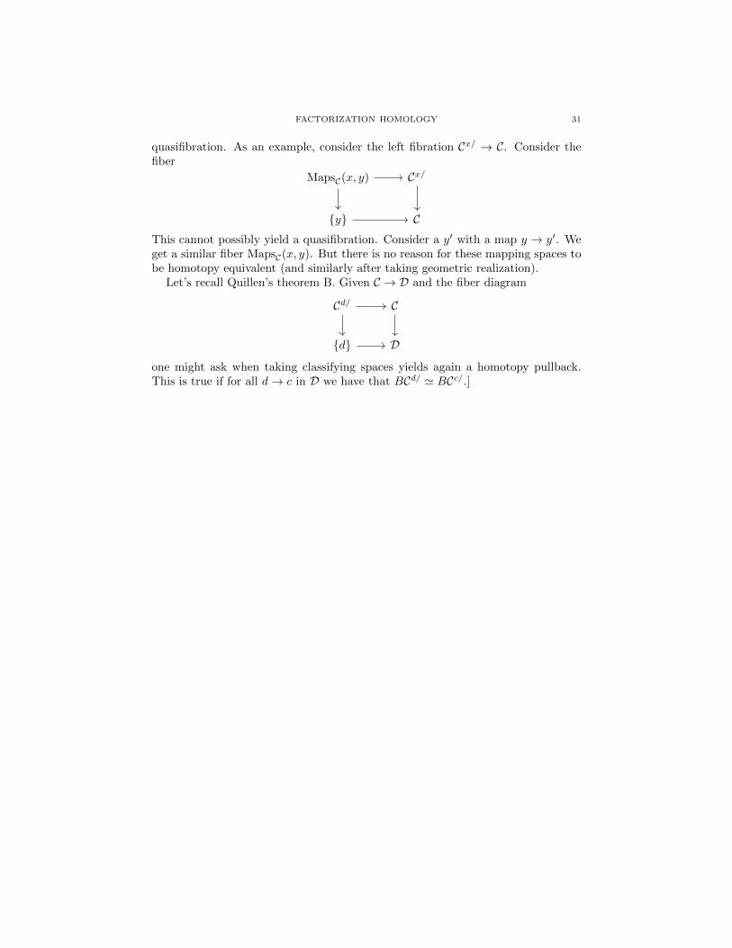
FACTORIZATION HOMOLOGY 31
quasifibration. As an example, consider the left fibration Cx/ → C. Consider thefiber
MapsC(x, y) Cx/
y CThis cannot possibly yield a quasifibration. Consider a y′ with a map y → y′. Weget a similar fiber MapsC(x, y). But there is no reason for these mapping spaces tobe homotopy equivalent (and similarly after taking geometric realization).
Let’s recall Quillen’s theorem B. Given C → D and the fiber diagram
Cd/ C
d D
one might ask when taking classifying spaces yields again a homotopy pullback.This is true if for all d→ c in D we have that BCd/ ' BCc/.]
32 FACTORIZATION HOMOLOGY
12. Homotopy invariance II [10/16/2017]
Today we’ll discuss the proof of the following fact, which was (1) in our outlineproof of homotopy invariance.
Corollary 49 (HTT 2.1.2.2). For all Kp−→ C the associated undercategory Cp/ is
a quasicategory.
Proof. We claim that Cp/ → C is a left fibration. Left implies inner, so composingwith the map to the point implies that Cp/ → C → ∆[0] is an inner fibration (it iseasy to check that compositions of fibrations are fibrations directly from the liftingproperty). We conclude that Cp/ is a quasicategory.
It remains to show that Cp/ → C is a left fibration, which we do below.
Recall from last time we had shown (if you include the homework) the following.
Lemma 50 (HTT 2.1.2.3). Given f : A0 → A, g : B0 → B with either f rightanodyne or g left anodyne then
A0 ? B∐
A0?B0
A ? B0 → A ? B
is inner anodyne.
This immediately implies
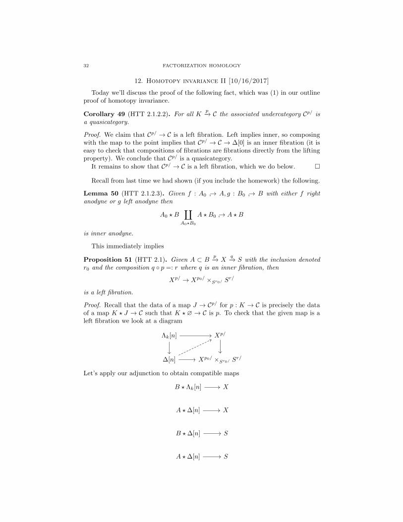
Proposition 51 (HTT 2.1). Given A ⊂ Bp−→ X
q−→ S with the inclusion denotedr0 and the composition q p =: r where q is an inner fibration, then
Xp/ → Xp0/ ×Sr0/ Sr/
is a left fibration.
Proof. Recall that the data of a map J → Cp/ for p : K → C is precisely the dataof a map K ? J → C such that K ? ∅ → C is p. To check that the given map is aleft fibration we look at a diagram
Λk[n] Xp/
∆[n] Xp0/ ×Sr0/ Sr/
Let’s apply our adjunction to obtain compatible maps
B ? Λk[n] X
A ?∆[n] X
B ?∆[n] S
A ?∆[n] S

FACTORIZATION HOMOLOGY 33
Putting these together,
B ? Λk[n] ∪A?Λk[n] A ?∆[n] X
B ?∆[n] S
and applying the lemma above, the vertical map on the left is inner anodyne,whence because X → S is an inner fibration, there exists a lift.
This concludes the proof that the undercategory is a quasicategory. To see this,we apply the proposition to the case where X = C, A = ∅, and B = ∗. HenceCp/ → C is a left fibration. Huh?
Sean: is there a time when it matters that these were left fibrations and notjust inner? John: absolutely. Think of inner as a technical condition but left/rightas a homotopy invariant property. In particular, every functor is equivalent to aninner fibration. This is not at all true for left fibrations. In particular, LFibD 'Fun(D,Spaces)—they’re like “fiber bundles with connection on D.”
Proposition 52 (HTT 1.2.5.1). For C a simplicial set the following are equivalent:
(1) C is a quasicategory and hC is a groupoid;(2) C → ∗ is a left fibration;(3) C → ∗ is a right fibration;(4) C → ∗ is a Kan fibration, i.e. C is a Kan complex.
If any of these are try we call C an ∞-groupoid or space.
Proposition 53 (HTT 1.2.4.3). A morphism φ : ∆[1]→ C in a quasicategory C isan equivalence if and only if for any extension f0 : Λ0[n]→ C
∆[1] C
Λ0[n]
∆[n]
φ
there is a lift to a map f : ∆[n]→ C.
Proof. By adjunction
0 C/∆[n− 2]
∆[0 < 1] C/∂∆[n− 2]
That proves one direction. For the other direction take a map φ : x→ y. We have
a filler Λ0[2] → ∆[2]ψ−→ C call it σ. This 2-simplex σ gives a homotopy idx ' ψ φ.
Show that φ ψ ' idy for homework.
This implies the equivalence of (1) ⇐⇒ (2) and dually (1) ⇐⇒ (2). But then(1) ⇐⇒ (2) + (3) = (4).

34 FACTORIZATION HOMOLOGY
13. Homotopy invariance III [10/18/2017]
Recall last time we wanted to prove Proposition 1.2.5.1.
Proof. To show that (1) =⇒ (2) notice that every ∆[1]→ C is a homotopy equiva-lence. Choose any f0
Λ[n] C
∆[n]
f0
and now by the previous proposition there exists an extension
∆[0 < 1]
Λ0[n] C
∆[n]
To see that (2) =⇒ (1) draw the same picture and apply the proposition, whichimplies that φ is an equivalence.
Notice that by taking opposites (1) ⇐⇒ (2) implies (1) ⇐⇒ (3), since takingopposites takes left fibrations to right fibrations. Hence (1) ⇐⇒ (2) + (3). Butbeing a left and right fibration is the same as being a Kan fibration, which completesthe proof.
Corollary 54. If C is a quasicategory there exists a maximal sub-Kan complex C0
whose morphisms consist of the homotopy equivalences in C.Figure out the HTT number.Fix the notation to tilde.
Proof. We can define C0 as the subsimplicial set with 1-simplices the homotopyequivalences. C0 is a quasicategory, and hC0 is a groupoid if and only if C0 is a Kancomplex.
In particular we have Kan ⊂ QCat ⊂ sSet and the construction in the corollaryis the right adjoint to the inclusion Kan → QCat.
Recall that our purpose was to show that colimits in quasicategories are invariant
with respect to categorical equivalence. In particular, given Jj−→ C p−→ D where p is
a categorical equivalence, we want to show that Cj/ ' Dpj/. We first needed theundercategories to be quasicategories. This we showed last time. Next we showthat the two horizontal arrows
Cj/ Dpj/ ×D C Dpj/
C
are equivalences. To see that the first is an equivalence we observe first that thevertical maps in the triangle are left fibrations, whence it is enough to show that it

FACTORIZATION HOMOLOGY 35
produces an equivalence on fibers. Thus we need the following. Given
C′ C′′
D
g
p
where g and h are left fibrations, we wish to show that p is an equivalence if andonly if C′d → C′′d is an equivalence of Kan complexes for all d ∈ D. To prove this it’seasiest to prove a slightly more general result. Then we need
Lemma 55 (HTT 2.5.4.1). Given J → C → D with the map from C to D anequivalence, then Cj/ ×C x → Dpj/ ×D px is an equivalence of Kan complexesfor all x ∈ C.
The following picture is good to keep in mind:
Kan fibration
left fibration right fibration
coCartesian fibration Cartesian fibration
inner fibration
Recall that an inner fibration is more of a technical condition rather than hav-ing some homotopy invariant meaning. Each of these fibrations (except for innerfibrations) are classified by functors to a representing object.
Example 56. Consider a functor F : [1] → Cat. Call F (0) = C, F (1) = D. Fromthis we can construct a categoryM = cyl(F ) := C×[1]
∐C×1D which sits over [1],
M→ [1]. This cylinder construction is a map Fun([1],Cat)→ Cat/[1]. You shouldthink of this as the most basic example of an “unstraightening construction”. Thecategories you obtain are the coCartesian fibrations over [1].
Definition 57. We say that a correspondence between two categories C and Dis a functor M→ [1] with M0
∼= C and M1∼= D.
This construction gives us correspondences but not all correspondences arise thisway. If we consider a span E from C to D we can produce a correspondence. Inparticular take the parameterized join C ?E D = C
∐E×0 E × [1]
∐E×1D over [1].
If our fibrations in our diagram above are over C (except for the inner fibration,say), then we get a diagram before unstraightening
Fun(C,Gpd0∞)
Fun(C,Gpd∞) Fun(C,Gpdop∞)
Fun(C,Cat∞) Fun(C,Catop∞)

36 FACTORIZATION HOMOLOGY
Note: unstraightening is also known as the “Grothendieck construction.” In par-ticular given F : C → Cat∞ then the fiber is just F (x) over x:
F (x) CF
x C
Corollary 58. Suppose we have a map C′ → C′′ of left fibrations over C, if C′ = CFand C′′ = CG (unstraightening) with the map of fibrations being induced by a naturaltransformation α sending F =⇒ G : C → Gpd∞. Then the map is an equivalence
if and only if α is an equivalence if and only if F (x)α−→ G(x) is an equivalence i.e.
C′x → C′′x is an equivalence.
We would have to prove a lot of this stuff to prove our fact, so we will probablytake it for granted.
Principle: any construction from category theory that only uses universal prop-erties goes through for ∞-categories.
The reason this unstraightening stuff is important because it’s generally easierto think about functors out of things instead of fibrations. On the other hand,fibrations (unstraightened things) are generally easier to construct.

FACTORIZATION HOMOLOGY 37
14. Back to topology [10/20/2017]
14.1. Finishing up homotopy invariance.
Lemma 59 (HTT 2.4.5.1). Given Kj−→ C p−→ D where p is an equivalence, we wish
to show that
Cj/ ×C x ' Dpj ×D px,for all x ∈ C.
Proof. We will induct on K. The base case is where K = c. In this case theleft hand side is MapsC(c, x) and the right hand side is Maps(pc, px). Hence weobtain an equivalence by assumption that C ' D. For the inductive step considerthe pushout
∂∆[n] Kα
∆[n] Kα+1
f
f
f
Write Cα = Cjα/ ×C x and Dα = Djαp/ ×D px, where jα is the restriction ofj to Kα → K. Now
Cjα+1/ = Cjα/ ×∂∆[n]/C C∆[n]/.
This implies that Cα+1 is the pullback
Cα+1 Cα
Cf Cf |∂∆[n]
Here Cf = C∆[n]/×C x. Now since C∆[n]/ → C∂∆[n]/ is a left fibration we find thatthe bottom arrow in the square above is a left fibration. However, both the sourceand the target are Kan complexes, whence the arrow is in fact a Kan fibration (thisis a lemma we will not prove—it is just a parameterized version of something wehave already proven). Draw the same diagram for D
Dα+1 Dα
Df Df |∂∆[n]
and note that by the inductive step Cα ' Dα and Cf ' Df . By induction we getequivalences which induce an equivalence Cα+1 ' Dα+1 because the bottom arrowsare Kan fibrations.
We will implicitly regard 1-categories as ∞-categories via the nerve.
14.2. Back to factorization homology.
Theorem 60. Let Spaces be the ∞-category of spaces and D iskn/M be the (nerveof) category of n-disks. Then∫
M
id := colim(D iskn/M
id−→ Spaces)'M

38 FACTORIZATION HOMOLOGY
Definition 61. An∞-category is κ-filtered, for κ some ordinal, if for any κ-smallK together with a functor K → C, there exists a factorization
K C
K.
For some intuition recall the analogous 1-categorical definition.
Definition 62. For C an ordinary category, we say that C is filtered if
(1) for any finite set xi of objects there exists an x such that there is a mapxi → x for all i,
(2) and for all f, g : x⇒ y there exists h : y → z such that hf = hg.
Example 63. As a simple example consider the category of natural numbers Nwith unique morphisms m→ n when m ≤ n. Condition (1) is clear and condition(2) is trivial due to the hom-sets being (at most) one-element sets.
Example 64. If C has a final object then C is filtered.
Example 65. Consider the subposet of open subsets of M that contain a fixedpoint p ∈ M , Opens(M)op
p ⊂ Opens(M)op. Notice that p wants to be a finalobject, but it need not be open. Let’s check that this is filtered. For any finitecollection Ui the intersection x = ∩IUi, gives us the first condition. Now supposewe have f, g : Ui → Uj . In this case we just let z = Uj : our category is a poset sof = g already. Hooray.
Lemma 66. If C is filtered as a 1-category then it is filtered as an ∞-category.
To see this, notice that any category can be built as a colimit in Cat from one-point categories.
Proof idea. Induct on K, building by coproducts and equalizers.
Filtered categories are nice because colimits indexed by them enjoy good prop-erties.
Lemma 67 (HTT 5.3.1.20). If C is filtered then BC ' ∗.
Recall that we are speaking model-independently—B is the left adjoint to theinclusion Spaces → Cat∞. In particular, given a map C → X for X a space itfactors uniquely up to homotopy through the classifying space.
If we think of quasicategories, it is the left-adjoint of the inclusion Kan → QCat.What does it do? Well it is a colimit-preserving functor, so we should describe iton the building blocks ∆[n]. By definition ∆[n] = N•([n]) where by [n] we think ofthe poset as a category. Define [n]′ to be the smallest groupoid with objects thatof [n].Wouldn’t this just be the
discrete groupoid?As a category, [n]′ ' ∗. Recall that ∆[n] is a quasicategory but not a Kan
complex. We send ∆[n] to N•([n]′).
FACTORIZATION HOMOLOGY 39
15. Computing factorization homology [10/25/17]
Goette, Igusa, Williams have a theorem (in the stable range): you get all exoticbundle structures through Hatcher’s construction. This is related to factorizationhomology. Anyway, back to filtered ∞-categories.
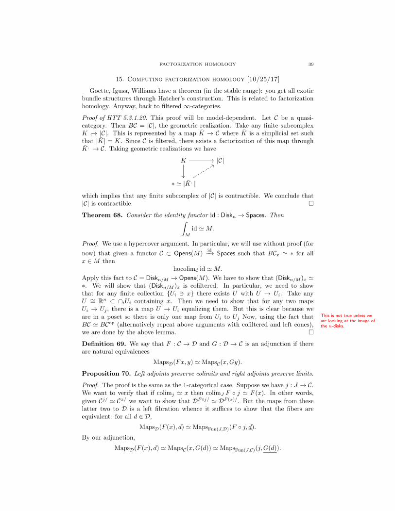
Proof of HTT 5.3.1.20. This proof will be model-dependent. Let C be a quasi-category. Then BC = |C|, the geometric realization. Take any finite subcomplexK → |C|. This is represented by a map K → C where K is a simplicial set suchthat |K| = K. Since C is filtered, there exists a factorization of this map throughK. → C. Taking geometric realizations we have
K |C|
∗ ' |K.|
which implies that any finite subcomplex of |C| is contractible. We conclude that|C| is contractible.
Theorem 68. Consider the identity functor id : Diskn → Spaces. Then∫M
id 'M.
Proof. We use a hypercover argument. In particular, we will use without proof (for
now) that given a functor C ⊂ Opens(M)id−→ Spaces such that BCx ' ∗ for all
x ∈M thenhocolimC id 'M.
Apply this fact to C = Diskn/M → Opens(M). We have to show that (Diskn/M )x '∗. We will show that (Diskn/M )x is cofiltered. In particular, we need to showthat for any finite collection Ui 3 x there exists U with U → Ui. Take anyU ∼= Rn ⊂ ∩iUi containing x. Then we need to show that for any two mapsUi → Uj , there is a map U → Ui equalizing them. But this is clear because weare in a poset so there is only one map from Ui to Uj This is not true unless we
are looking at the image ofthe n-disks.
Now, using the fact thatBC ' BCop (alternatively repeat above arguments with cofiltered and left cones),we are done by the above lemma.
Definition 69. We say that F : C → D and G : D → C is an adjunction if thereare natural equivalences
MapsD(Fx, y) ' MapsC(x,Gy).
Proposition 70. Left adjoints preserve colimits and right adjoints preserve limits.
Proof. The proof is the same as the 1-categorical case. Suppose we have j : J → C.We want to verify that if colimj ' x then colimJ F j ' F (x). In other words,
given Cj/ ' Cx/ we want to show that DFj/ ' DF (x)/. But the maps from theselatter two to D is a left fibration whence it suffices to show that the fibers areequivalent: for all d ∈ D,
MapsD(F (x), d) ' MapsFun(J,D)(F j, d).
By our adjunction,
MapsD(F (x), d) ' MapsC(x,G(d)) ' MapsFun(J,C)(j,G(d)).
40 FACTORIZATION HOMOLOGY
ButMapsFun(J,C)(j,G(d)) ' lim
z∈JopMapsC(jz,Gd)
andMapsFun(J,D)(F j, d) ' lim
z∈JopMapsD(Fjz, d),
which are the same by our adjunction.Notice that this is a model independent proof.
The following is an important adjunction (of∞-categories) to keep in mind. Thesingular chains C∗ : Spaces → Ch has a right adjoint G such that π∗GV is H∗Vfor ∗ ≥ 0 and 0 otherwise. This comes from the adjunction between sSet and sAbgiven by free abelian group and forgetful funtors. Hence C∗ preserves (homotopy)colimits.
Notice that there exists a unique colimit preserving functor F : Spaces → Vfor V any ∞-category with colimits with F (∗) = v since any space is built as a
colimit of contractible spaces. In particular, any X = colim(U j−→ Spaces) whereu 7→ ju ' ∗, which yields the same colimit as the constant diagram U → V andF (X) = colim(U → V).
Let’s do another calculation. Consider the functor Z⊕ : Diskn → Ch sending∐I Rn 7→ Z⊕I . Let’s calculate
∫M
Z⊕. Notice first that Z⊕I ' C∗(∐I Rn). Hence∫
M
Z⊕ '∫M
C∗ id = colim(
Diskn/Mid−→ Spaces
C∗−−→ Ch).
Since C∗ is colimit preserving,∫M
Z⊕ ' C∗ colim(
Diskn/Mid−→ Spaces
)' C∗
∫M
id ' C∗M.
Similarly for those of you familiar with spectra, there is a adjunction of spaces withspectral given by Ω∞ and Σ∞∗ and exactly the same proof shows that∫
M
S⊕ ' Σ∞∗ M.
Definition 71. Let Disk=1n ⊂ Diskn be those n-disks with |I| = 1.
Now repeating the arguments of this lecture for this subcategory, we find
colim(
Disk=1n /M
id−→ Spaces)'M.
In other words, it is enough to probe manifolds with single-opens. However, all ofthis seeming differential topology washes out.
Proposition 72. There is an equivalence of ∞-categories D isk=1n /M ' M . Or as
quasicategories, D isk=1n /M ' Sing(M).
Proof sketch. We construct a functor ev0 given by evaluation at 0 sending φ : Rn →M 7→ φ(0) ∈ M . This functor induces an equivalence on objects so it remains tocheck on mapping spaces. In particular, need to check MapsD iskn/M
(Rn,Rn) 'ΩM .
Now using that Diskn/M → D iskn/M is a localization, we find that colimM ∗ 'M .

FACTORIZATION HOMOLOGY 41
16. Nonabelian Poincare duality I [10/27/2017]
Example 73. Recall we have the free En-algebra on a space Z, A = F (Z). Thisfunctor A : Diskn → Spaces sends
U 7→∐i>0
Confi(U)×Σi Zi.
Proposition 74. The factorization homology of A is∫M
F (Z) =∐i>0
Confi(M)×Σi Zi.
We will need the following lemma.
Lemma 75. The map from the homotopy colimit
colimU∈Diskn/M
Confi(U)∼−→ ConfI(M)
is a homotopy equivalence.
Proof. We have Diskn/M → Opens(M)Confi−−−−→ Spaces which we can look at as
Diskn/MConfi−−−−→ Opens(Confi(M))
id−→ Spaces.
Apply our hypercover lemma to this line: we need to check that for each x1, . . . , xi ∈Confi(M), Diskn/M,x1,...,xi has a contractible classifying space. We have alreadydone this in the case when i = 1. In particular, we just check that the categoryis cofiltered—perform the argument before for each point. Let’s check the twoconditions: given any finite collection of Uj containing the x1, . . . , xi, there existsU ⊂ ∩jUj (the intersection itself is not a disjoint union of disks) with U → Ujfor all j. The second condition is again trivial by the fact that our category is aposet.
Notice that this lemma holds for Confi(U) ×Σi Zi, which we will use below.
Alternatively one might use the fact that products commute with colimits. Inparticular colimJ Z × Fj → Z × colimj∈J Fj is an equivalence.
Proof of proposition. Formally, colimits commute so we have
colimU∈Diskn/M
∐i>0
Confi(M)×Σi Zi =
∐i≥0
colimU∈Diskn/M
(Confi(U)×Σi Z
i)
'∐i>0
(colim
U∈Diskn/MConfi(M)
)×Σi Z
i
'∐i>0
Confi(M)×Σi Zi,
as desired.
This proof is written down in the paper [AF15] of Ayala and F.Let’s turn to a more complicated example. Recall that we have a functor
DisknMapsc(−,Z)−−−−−−−−→ Spaces for Z a pointed space. We have a natural map
colim
(Diskn/M
Mapsc(−,Z)−−−−−−−−→ Spaces
)→ colim
(Mfldn/M
Mapsc(−,Z)−−−−−−−−→ Spaces
)

42 FACTORIZATION HOMOLOGY
identifying the n-disks as manifolds. Notice that the colimit on the right hand sidehas a category with a final object as its source, whence the colimit is equivalent toMapsc(M,Z). This leads us to the following theorem, due to Segal, Salvatore, andLurie, in various formulations.
Theorem 76 (Nonabelian Poincare duality). Let M be an n-manifold and Z bean (n− 1)-connected pointed space. Then the map defined above∫
M
Mapsc(−, Z)∼−→ Mapsc(M,Z)
is an equivalence.The name comes from thefact that if one takes Z to
be an Eilenberg-Maclanespace, then recover the usual
statement of Poincareduality.
Remark 77. Let’s see why we need the condition that π∗Z = 0 for ∗ < n. Let’sfirst consider the case where Z = S0. Let’s look at the left-hand side:
colimU∈Diskn/M
Mapsc(U, S0) ' B(Diskn/M )
which is connected because between any two objects there is a morphism. Now let’slook at Mapsc(M,S0) for M compact. But now Mapsc(M,S0) = Maps(M,S0) hasat least 2 components for M 6= ∅.
More formally, note that Mapsc(Rn, Z) ' ΩnZ. But using the long exact se-quence on the homotopy groups of a fibration repeatedly, we compute
π∗ΩnZ = π∗+nZ for ∗ > 0.
In particular, this does not depend on π∗Z for ∗ < n. So this statement couldnot possibly be true because we could just change the space such that only the
< n homotopy groups change. In particular, take τ≥nZhofiber−−−−→ Z → Pn−1Z where
Pn−1Z is the n− 1 Postnikov stage:
Mapsc(Rn, Z) ' Mapsc(Rn, τ≥nZ).
So the functor on the left will not change, but the functor on the right can alwaysdetect these by choosing M appropriately. This tells us that we had better chooseZ ' τ≥nZ.
Grisha: does the left hand side depend on the map M → BO(n). John: No, inparticular Diskn/M only knows about the homeomorphism type of M . Morevoer
there is a cancellation of sorts Disknfr/M ' Diskn/M . Again, this is something you
can find in the paper [AF15].We can think of both sides as functors out of Mfldn. Given a natural trans-
formation between to functors out of here, to show it is an equivalence, we mightfirst show that it is an equivalence on Rn, and then show that the functors sat-isfy the same “gluing/cosheaf” properties. In particular, do these functors satisfysomething like Mayer-Vietoris?
To prove such a property, one might “filter” either Z or M . Jacob, in his book,does the former (via Postnikov stages), while John does it by breaking down M .We’ll be doing the latter.
Definition 78. For V a symmetric monoidal ∞-category, a homology theoryfor n-manifolds valued in V is a symmetric monoidal functor
F : (Mfldn,∐
) (V,⊗)

FACTORIZATION HOMOLOGY 43
such that whenever M ∼= M ′∐M0×RM
′′ for dimM0 = n− 1 then
F (M ′)⊗F (M0×R) F (M ′′)→ F (M)
is an equivalence.
Theorem 79. If we write the collection H(Mfldn,V) for all such homology theo-ries, then there is an equivalence
H(Mfldn,V) AlgDiskn(V)
evDiskn
∫−
Theorem 80. Mapsc(−, Z) and∫−Mapsc(−, Z) are homology theories valued in
Spaces.
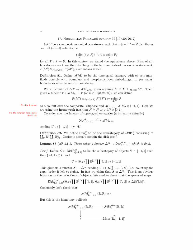
44 FACTORIZATION HOMOLOGY
17. Nonabelian Poincare duality II [10/30/2017]
Let V be a symmetric monoidal ∞-category such that v⊗− : V → V distributesover all (sifted) colimits, i.e.
colimJ
(v ⊗ Fj)∼=−→ v ⊗ colim
JFj
for all F : J → V. In this context we stated the equivalence above. First of all:how do we even know that the thing on the left hand side of our excision statement,F (M ′)⊗F (M0×R) F (M ′′), even makes sense?
Definition 81. Define M fld∂n to be the topological category with objects man-ifolds possibly with boundary, and morphisms open embeddings. In particular,boundaries must be sent to boundaries.
We will construct ∆op → M fldn/M given a gluing M ∼= M ′ ∪M0×R M′′. Then,
given a functor F : M fldn → V (or into (Spaces,×)), we can define
F (M ′)⊗F (M0×R) F (M ′′) := colim∆op
F
as a colimit over the composite. SupposeFix this diagram and M |(−1,1)∼= M0 × (−1, 1). Here we
are using the homework fact that N ∼= N ∪∂N ∂N × [0, 1).Fix the notation here, make
the D calConsider now the functor of topological categories (a bit subtle actually)
Disk∂1/[−1,1]π−1
−−→M fldn/M
sending U → [−1, 1] 7→ π−1U .
Definition 82. We define Disk∂n to be the subcategory of M fld∂n consisting of∐U Rn
∐j Rn≥0. Notice it doesn’t contain the disk itself.
Lemma 83 (AF 3.11). There exists a functor ∆op → Disk∂,or1/[−1,1] which is final.
Proof. Define S ⊂ Disk∂,or1/[−1,1] to be the subcategory of objects U ⊂ [−1, 1] such
that −1, 1 ⊂ U and
U = [0, ε)∐
R∐l∐
(δ, 1] → [−1, 1].
This gives us a functor S → ∆op sending U 7→ π0([−1, 1] \ U), i.e. counting thegaps (order it left to right). In fact we claim that S ' ∆op. This is an obviousbijection on the collections of objects. We need to check that the spaces of maps
Disk∂,or1/[−1,1]([0, ε)
∐R
∐i∐
(δ, 1], [0, ε′)∐
R∐i′∐
(δ′, 1]) ' ∆([i′], [i]).
Concretely, let’s check that
Mfld∂,or1/[−1,1](R,R) ' ∗.
But this is the homotopy pullback
Mfld∂,or1/[−1,1](R,R) Mfld∂,or
1 (R,R)
∗ Maps(R, [−1, 1])

FACTORIZATION HOMOLOGY 45
by definition of∞-categorical overcategories. But the two spaces on the right handside are contractible, hence we obtain what we wanted. This implies the discretenessand hence the equivalence of the mapping spaces.
Let us check that the functor is final. We use Quillen’s theorem A. In particular,
we show that B(SV/ ' ∗ for V ∈ Disk∂,or1/[−1,1]. We have
V = [0, ε)∐
?∐
R∐i∐
(δ, 1)∐
?.
If V ∈ S then SV/ has an initial object whence BSV/ ' ∗. On the other hand, ifV ∈ S has neither 0 nor 1 then
V ′ = V∐
[0, ε)∐
(δ, 1]
is initial in SV/. Indeed, we claim that given any W ⊂ [−1, 1] and an embeddingV → W , the space of factorizations through V ′ is contractible. But this is justthat
Mfld/[−1,1]([0, ε), [0, ε′)) ' ∗.
Hence S is final.
Now, given M ′ ∪M0×R M′′, and a functor F : M fldn → V, we define
F (M ′)⊗F (M0×R) F (M ′′) = colim∆op
F
where the functor is the composite
∆op →Mfld∂,or1/[−1,1] →M fldn → V,
which if F is symmetric monoidal then this is just a two-sided bar construction.Sam: why did we do this construction instead of just writing it as a bar con-
struction in the first place? John: this is not just a normal simplicial object. It’sa simplicial object in an ∞-category. Indeed, there is no functor ∆op → Mfldn/M .We are useful a flexibility of isotopies and contractibilities to actually build thisobject.
Now, if A is an n-disk algebra in V, we would like to show that∫−A is a ⊗-
homology theory, i.e. ∫M ′
A⊗∫M0×R A
∫M ′′
A '∫M
A.
In fact we will prove something stronger. We will write down a pushforward formula.Say we are given f : M → (N, ∂N) with M |int(N) → int(N) and M |∂N → ∂N fiberbundles.
Theorem 84. Given the pushforward
f∗A : Disk∂n/Nf−1
−−→M fldn/M
∫A−−→ V,
there is an equivalence ∫M
A '∫N
f∗A.
This will imply that factorization homology is a ⊗-homology theory.
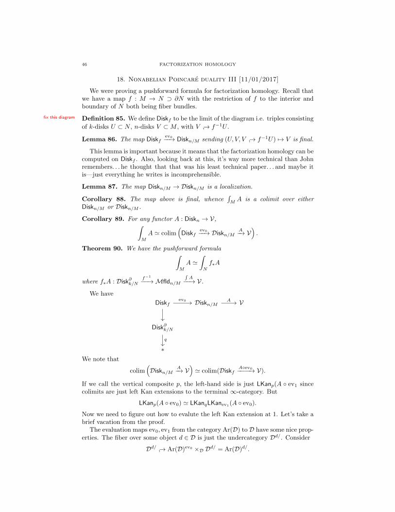
46 FACTORIZATION HOMOLOGY
18. Nonabelian Poincare duality III [11/01/2017]
We were proving a pushforward formula for factorization homology. Recall thatwe have a map f : M → N ⊃ ∂N with the restriction of f to the interior andboundary of N both being fiber bundles.
Definition 85. We define Diskf to be the limit of the diagramfix this diagram i.e. triples consisting
of k-disks U ⊂ N , n-disks V ⊂M , with V → f−1U .
Lemma 86. The map Diskfev0−−→ Diskn/M sending (U, V, V → f−1U) 7→ V is final.
This lemma is important because it means that the factorization homology can becomputed on Diskf . Also, looking back at this, it’s way more technical than Johnremembers. . . he thought that that was his least technical paper. . . and maybe itis—just everything he writes is incomprehensible.
Lemma 87. The map Diskn/M → Diskn/M is a localization.
Corollary 88. The map above is final, whence∫MA is a colimit over either
Diskn/M or Diskn/M .
Corollary 89. For any functor A : Diskn → V,∫M
A ' colim(
Diskfev0−−→ Diskn/M
A−→ V).
Theorem 90. We have the pushforward formula∫M
A '∫N
f∗A
where f∗A : Disk∂k/Nf−1
−−→Mfldn/M
∫A−−→ V.
We have
Diskf Diskn/M V
Disk∂k/N
∗
ev0 A
q
We note that
colim(Diskn/M
A−→ V)' colim(Diskf
Aev0−−−−→ V).
If we call the vertical composite p, the left-hand side is just LKanp(A ev1 sincecolimits are just left Kan extensions to the terminal ∞-category. But
LKanp(A ev0) ' LKanqLKanev1(A ev0).
Now we need to figure out how to evalute the left Kan extension at 1. Let’s take abrief vacation from the proof.
The evaluation maps ev0, ev1 from the category Ar(D) to D have some nice prop-erties. The fiber over some object d ∈ D is just the undercategory Dd/. Consider
Dd/ → Ar(D)ev0 ×D Dd/ = Ar(D)d/.

FACTORIZATION HOMOLOGY 47
This map is a left adjoint. The right adjoint is simple: just compose. John: check this for yourself.On the otherhand,
D/d → Ar(D)ev1 ×D D/dis a right adjoint (again the other is given by composition). Now recall that leftadjoints are initial functors and right adjoints are final. Observe that given π :A → D such that Ad → A/d = A×D D/d is final for any d, then
LKanπF ' colimA/d
F ' colimAd
F.
Definition 91. Such a functor π is called a locally Cartesian fibration.
What we have seen above is that evaluation at 0 and 1 are locally coCartesianand Cartesian fibrations.
Returning from our vacation (which are never as relaxing as you expect) we findthat by the Cartesian fibration property,
LKanev0(A ev1)(U) ' colim(Diskf |U
Aev0−−−−→ V).
But Diskf |U = Diskn/f−1U . Hence we find
LKanev0(A ev1)(U) = colim(Diskn/f−1UA−→ V) =
∫f−1U
A =: f∗A(U).
But now∫MA '
∫Nf∗A, which completes the proof (using the finality of the
localization).There is a bit of a gap here: we used the locally Cartesian fibration property.
However, really what we had was a pullback of a locally Cartesian fibration property.Unfortunately, this property is not preserved under pullbacks. However we are okbecause we have Cartesian, not just locally Cartesian.
What’s left is two lemmas. The localization result and the finality result.
Lemma 92. The map ev0 : Diskf → Diskn/M is final.
Proof. We use Quillen’s theorem A, which says that F → D is final if B(Fd/) ' ∗for all d ∈ D. So for any V ∈ Diskn/M we need to check that B(Disk
V/f ) ' ∗. Recall
that ev0 is a (locally) Cartesian fibration. This means that the fiber of ev0 includedinto the undercategory
Diskf |V → DiskV/f
is a left adjoint. Now we recall that if we are given an adjunction between Cand D by F and G. This implies an equivalence of classifying spaces BC ' BD(just a special case of being final or initial since the classifying space functor is acolimit of the constant functor; alternatively just look at how the unit/counit mapsgive you homotopies). This implies that we can show instead that the fiber overV , Diskf |V , has contractible classifying space. This category consists of k-disksU ⊂ N with V → f−1U . We don’t have much time left, but the basic idea is touse the hypercover argument.
Yajit: how to make the “colliding points” picture of factorization homologyprecise? John: consider the subcategory Disksurj
n/M ⊂ Diskn/M which is surjective on
π0. This subcategory is the exit-path infinity category of the Ran space Ran(M).But Fun(Exit(RanM),V) are constructible cosheaves on Ran(M), and then
∫MA =
Γ(Ran, A).

48 FACTORIZATION HOMOLOGY
19. Nonabelian Poincare duality IV [11/03/2017]
Proposition 93 (AF 2.19). The map Diskn/M → Diskn/M is a localization, i.e.Diskn/M is the universal ∞-category under Diskn/M such that isotopy equivalencesto equivalence. More precisely, for any functor Diskn/M → C sending isotopy equiv-alences to equivalences, there exists a unique factorization through Diskn/M .
There are two parts: a formal criterion for localizations, and a topological ar-gument via hypercovers. Let’s look at the former. Here’s a naive guess: a functorC → D a localization with respect to I ⊂ C if the space of objects of D = BI. If, sayI was the underlying groupoid of C (the trivial localization), then this checks out.
Moreover, for the space of morphisms take B(FunI([1], C
). Likewise for p-tuples
(not just spans). This is a sufficient condition.
Proof. We check that the space of objects is that of a localization. The rest can befound in the paper. In particular we check that
B Funiso eq([p],Diskn/M ) ' Maps([p],Diskn/M )
for p = 0. In this case the left hand side is Diskiso eqn/M which is just
∐k≥0(Disk=k
n/M )iso eq
and the right hand side is the underlying groupoidDiskn/M which is just∐k≥0(Disk=k
n/M )0.Change the underlying
groupoid notation.Let’s start with the right hand side. For k = 1 it has objects Rn → M so
Disk=1n/M ' M where we think of M as an ∞-groupoid. The functor giving the
equivalence is given by evaluation at 0 (one needs to actually check that this is afunctor). To check that it’s an equivalence we check that
Emb/M (φ : Rn →M,ψ : Rn →M) ' MapsM (φ(0), ψ(0))
= γ : [0, 1]→M | γ(0) = φ(0), γ(1) = ψ(0).The left hand side is the homotopy fiber
Emb/M (φ, ψ) Emb(Rn,Rn)
∗ Emb(Rn,M)
The top right is O(n) and the bottom right is the frame bundle of the tangentbundle. But the homotopy fiber of the inclusion of the fiber into the frame bundleis, by the Puppe sequence, just ΩM . That’s exactly the right hand side. Thisproves it for k = 1.
For general k, the evaluation at 0 maps to the unordered configuration spaceConfk(M)Σk . Apply the exact same argument as the k = 1 case. Hence
Disk0n/M '
∐k≥0
Confk(M)Σk .
We want to modify our hypercover argument from earlier to tell us that
colimDisk=k,iso eq
n/M
(Rn)kΣk∼−→ Confk(M)Σk
is an equivalence. Notice that it is important that the k’s on the left and the right
are the same. But (Rn)k ' ∗ whence the colimit is equivalent to B(Disk=k,iso eqn/M '
Confk(M)Σk ' Disk=k, iso eqn/M .

FACTORIZATION HOMOLOGY 49
This is a handy result which, since localizations are both final and initial, allowsus to compute factorization homology along either category.
Lemma 94 (AF 3.21). With f,M,N as in last lecture, the map Diskf → Disk/Mis final.
Proof. We use Quillen’s theorem A: show B(DiskU/f )U→M ' ∗. Notice that we have
Disk∂k/Nf−1
−−→Mfldn/MEmb/M (U,−)−−−−−−−−→ Spaces
and as a general feature of unstraightening,
B(DiskU/f ) = colim
Disk∂k/N
Emb/M (U, f−1V )
The right hand side is equivalent to ∗ since
colimDisk∂
k/N
Emb(U, f−1V )'−→ Emb(U,M).
Okay, so since I’ve lost basically all of you, I’ll simplify the proof and finish theproof in the case of Embfr. We need to show that
colimDisk∂
k/N
Embfr(U, f−1V )→ Embfr(U,M).
Replace the index category with Disk∂k/N by the proposition above. We thus need
to show that we have an equivalence
colimDisk∂
k/N
Confπ0U (f−1V ) → open Confπ0U (M).
Now we apply the hypercover argument. Set |π0U | = K. For points x1, . . . , xk ∈Confk(M), want to show B(Disk∂k/N )x1,...,xk) ' ∗. First we check that it’s
nonempty. Notice under f these points get sent to fx1, . . . , fxk ∈ Nk. Wecan choose k little disks containing these images, call it V . Take the inverse imageof V and this inverse image will now contain the disk. The argument that thecategory is cofiltered goes as usual.
For the non-framed case, the argument is similar, which you can find the in thepaper.
Sam: we’re showing localization for handles of index 0. Can we do this for higherindex handles? John: If you enhance by some stratification story, yes. Otherwisethere’s an issue about convergence of the Goodwillie-Weiss tower.
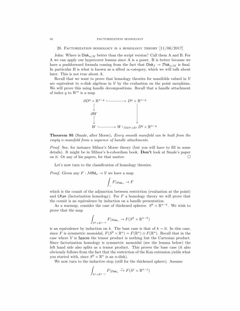
50 FACTORIZATION HOMOLOGY
20. Factorization homology is a homology theory [11/06/2017]
John: Where is Diskn/M better than the script version? Call them A and B. ForA we can apply our hypercover lemma since A is a poset. B is better because wehave a pushforward formula coming from the fact that Diskf → Diskn/M is final.In particular B is what is known as a sifted ∞-category, which we will talk aboutlater. This is not true about A.
Recall that we want to prove that homology theories for manifolds valued in Vare equivalent to n-disk algebras in V by the evaluation on the point morphism.We will prove this using handle decompositions. Recall that a handle attachmentof index q to Wn is a map
∂Dq × Rn−q Dq × Rn−q
∂W
W W ∪∂Dq×Rq Dq × Rn−q
Theorem 95 (Smale, after Morse). Every smooth manifold can be built from theempty n-manifold from a sequence of handle attachments.
Proof. See, for instance Milnor’s Morse theory (but you will have to fill in somedetails). It might be in Milnor’s h-cobordism book. Don’t look at Smale’s paperon it. Or any of his papers, for that matter.
Let’s now turn to the classification of homology theories.
Proof. Given any F :Mfldn → V we have a map∫−F |Diskn → F
which is the counit of the adjunction between restriction (evaluation at the point)and LKan (factorization homology). For F a homology theory we will prove thatthe counit is an equivalence by induction on a handle presentation.
As a warmup, consider the case of thickened spheres: Sk × Rn−k. We wish toprove that the map ∫
Sk×Rn−kF |Diskn → F (Sk × Rn−k)
is an equivalence by induction on k. The base case is that of k = 0. In this case,since F is symmetric monoidal, F (S0 × Rn) = F (Rn)⊗ F (Rn). Recall that in thecase where V is Spaces the tensor product is nothing but the Cartesian product.Since factorization homology is symmetric monoidal (see the lemma below) theleft hand side also splits as a tensor product. This proves the base case (it alsoobviously follows from the fact that the restriction of the Kan extension yields whatyou started with, since S0 × Rn is an n-disk).
We now turn to the inductive step (still for the thickened sphere). Assume∫Sj×Rn−j
F |Diskn∼−→ F (Sj × Rn−j)

FACTORIZATION HOMOLOGY 51
is an equivalence for j < k. We use that we can write Sk × Rn−k = Rk+ ×Rn−k ∪Sk−1×R×Rn−k Rk− × Rn−k. Now apply our excision result∫
Sk×Rn−kF |Diskn '
∫Rk+×Rn−k
F |Diskn ⊗Sk−1×R×Rn−k
∫Rk−×Rn−k
F |Diskn
and notice that
F (Sk × Rn−k) ' F (Rk+ × Rn−k)⊗F (Sk−1×R×Rn−k) F (Rk− × Rn−k).
Applying the induction hypothesis to what we are taking the tensor product over,and applying homotopy invariance of this tensor product (recall that it was definedas a homotopy colimit), we obtain the desired equivalence. This completes theproof for thickened spheres.
Now let’s turn to a general sequence of handle attachments starting from theempty set. Inductively, we assume the counit map is an equivalence for k − 1 andwe show it for k. Look at the diagram for W above in our description of Smale’stheorem. By the inductive hypothesis, for W with fewer than k-handles,∫
W
F |Diskn∼−→ F (W )
and similarly for (a thickened version of) the manifold on the top left and themanifold on the top right. Now applying the ⊗-excision principle and the inductionhypothesis concludes the proof.
Lemma 96. For A ∈ AlgDiskn(V), the factorization homology is symmetric monoidalif ⊗ in V preserves colimits.
Proof. Consider the composite
Diskn/MtN Diskn/M ×Diskn/N V × V V∼ A×A ⊗
Then since ⊗ preserves colimits∫MtN
A ' colim(Diskn/M ×Diskn/N
⊗A×A−−−−−→ V)
' ⊗ colim(Diskn/M ×Diskn/N → V × V
)'∫M
A⊗∫N
A.
Lemma 97. For Z an n-connective pointed space, the functor Mfldn → Spacessending M 7→ Mapsc(−, Z) is a ×-homology theory.
Remark 98. There is an equivalence of infinity-categories, for G any topologicalgroup,
Spaces/BG ' G− Spaces.
More generally, there is an equivalence LFibC ' Fun(C,Spaces). But we can deduceit more directly—in more point-set terms the left hand side is considered as spacesthat are fibrations over BG and the right hand side as G-spaces where the G-actionis free. There is a map from the right to the left taking quotients, and the mapfrom the left to the right is taking the fiber above the distinguished point overBG. If we omit the words fibration/free we replace quotient/fiber with homotopyquotient/homotopy fiber. The reason this is true is that taking homotopy fibers

52 FACTORIZATION HOMOLOGY
preserves homotopy colimits.1 Suppose we are given a space E → BG with fiberF . There is a map F ×G EG → E over BG. Hence we have a map of twohomotopy fiber sequences, so the LES in homotopy groups for a fibration shows usthat π∗E ∼= π∗F ×G EG. Hence every space over BG is the fiber of the quotient ofthe induced action of G. Similarly for the converse: if G acts on F then the fiberof FG → BG is just F again.
21. Nonabelian Poincare duality VI [11/08]
Nilay: could you quickly go over again how the pushforward formula implies⊗-excision of factorization homology? John: Sure. Choose a map M → [−1, 1]that exhibits the decomposition of M into M ′ and M ′′ (there’s a diagram we drewbefore). The pushforward formula tells us that∫
[−1,1]
f∗A =
∫M
A
and we used finality to pass from a colimit over Disk partial or over [−1, 1] to acolimit over ∆op to reduce to the two-sided bar construction which is precisely the⊗-excision.
We now return to the proof of nonabelian Poincare duality. Recall the n-diskalgebra ΩnZ := Mapsc(Rn, ), for Z an n-connective pointed space.
Proof. We just need to show that Mapsc(−, Z) is a ×-homology theory in Spacesand then apply our classification of ⊗-homology theories to conclude that it is givenby factorization homology. In other words in suffices to prove the last lemma fromlast lecture.
Learn the 2-sided barconstruction.
Proof. Choose a decomposition M ∼= M ′ ∪M0×R M′′. We need to show that the
natural map Mapsc(M′, Z)×Mapsc(M
′′, Z))Mapsc(M0×R,Z) → Mapsc(M,Z). is anequivalence. The source is the quotient by the E1-algebra, Mapsc(M0 × R, Z), inSpaces where the structure is given by the monoidal map
Disk1M0×−−−−−→Mfldn
Mapsc(−,Z)−−−−−−−−→ Spaces.
Observe thatM0 →M is proper, whence we obtain a restriction map Mapsc(M,Z)→Mapsc(M0, Z). Observe that this restriction map is a Serre fibration with a con-nected base because Z is n-connective and M0 is (n − 1)-dimensional (every mapin the base is homotopic to the constant map). Let’s look at the fibers of this map.
Mapsc((M,M0), (Z,Z∗)) Mapsc(M,Z)
∗ Mapsc(M0, Z)M0→∗→Z
However, this space of compactly supported maps of pairs is
Mapsc((M,M0), (Z, ∗)) ' Mapsc(M \M0, Z).
Recall that this is the same argument as ΩnZ ' Mapsc(int(Dn), Z). Finally, notice
that M \M0∼= M ′ tM ′′ (shrinking collars).
1Check, for instance, that taking set-theoretic fibers preserves colimits along closed inclusions.

FACTORIZATION HOMOLOGY 53
Since the bottom right of the square is a connected space we find
Mapsc(M′ tM ′′, Z)Ω Mapsc(M0,z)
∼−→ Mapsc(M,Z)
from the equivalence of ΩK−Spaces with Spaces/K for K connected (for which we
have B ' B(ΩK) and G ' ΩBG). Now, since, Ω Mapsc(M0, Z) ' Mapsc(M0 ×R, Z) and since compactly supported maps functor sends disjoint unions to prod-ucts, we obtain the desired result.
This completes the proof of nonabelian Poincare duality.Matt: how difficult is the hypercover lemma? John: I wouldn’t think of it as
too difficult. There’s a proof in Jacob’s appendix of hypercovers. A better place tostart is Segal’s Classifying Spaces paper, which has the essential idea. Then variousglossed up versions are due to Dugger and Isaaksen.
Remark 99. Nonabelian Poincare duality in this form is the best route to computingH∗Mapsc(M,Z) when M is a manifold. Of course, factorization homology looksa lot more complicated than this but on the plus side, it has a lot more handlesattached.
Example 100. Let Z = ΣnK for K connected. We know
C∗Mapsc(M,ΣnK) '∫M
C∗(ΩnΣnK) = ⊕i≥0C∗
(Confi(M)×Σi K
∧i)since the argument is a free n-disk algebra in chain complexes. How would you dothis otherwise? Even Sam is allowed to contribute. This is a hard problem.
Sam: rational homotopy theory? John: hmm. . . okay, but that depends onsimply-connectedness and characteristic zero.
However, this result predates factorization homology, c.f. McDuff, Segal, Boedigheimer.
Remark 101. Let’s quickly look at why nonabelian Poincare duality reduces toPoincare duality. Let Z = K(A, i), with i ≥ n. Consider
πj Mapsc(M,K(A, i)) ∼= [M,ΩjK(A, i)]c ∼= Hi−jc (M ;A),
so we have cohomology on the right hand side. On the other side we have∫M
ΩnK(A, i).
This takes some arguing that we haven’t done but I’ll tell you the end result. Thereis the Dold-Kan functor followed by geometric realization DK : Ch→ Spaces sendingA[i] 7→ K(A, i). Now recall that∫
M
V ' C∗(M,V )
for a chain complex V . Set V to be A[i− n]. Hence∫M
ΩnK(A, i) ' |C∗(M,A[i− n])|.
Nilay: what happened to orientation? John: notice that these are n-disk alge-bras, and not En-algebras. In particular there is a nontrivial action of O(n) onK(A, i). The Z/2 of the components of O(n) is giving us the orientation twist. Inparticular, the left hand side yields the twisted homology.
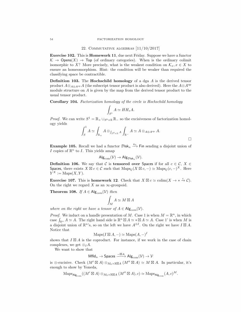
54 FACTORIZATION HOMOLOGY
22. Commutative algebras [11/10/2017]
Exercise 102. This is Homework 11, due next Friday. Suppose we have a functorK → Opens(X) → Top (of ordinary categories). When is the ordinary colimitisomorphic to X? More precisely, what is the weakest condition on Kx, x ∈ X toensure an homeomorphism. Hint: the condition will be weaker than required theclassifying space be contractible.
Definition 103. The Hochschild homology of a dga A is the derived tensorproduct A⊗A⊗AopA (the subscript tensor product is also derived). Here the A⊗Aop
module structure on A is given by the map from the derived tensor product to theusual tensor product.
Corollary 104. Factorization homology of the circle is Hochschild homology∫S1
A ' HH∗A.
Proof. We can write S1 = R+ ∪S0×R R− so the excisiveness of factorization homol-ogy yields ∫ 1
S
A '∫R+
A⊗∫S0×R A
∫R−
A ' A⊗A⊗Aop A.
Example 105. Recall we had a functor Disknπ0−→ Fin sending a disjoint union of
I copies of Rn to I. This yields amap
Algcom(V)→ AlgDiskn(V).
Definition 106. We say that C is tensored over Spaces if for all c ∈ C, X ∈Spaces, there exists X c ∈ C such that MapsC(X c,−) ' MapsC(c,−)X . HereY X := Maps(X,Y ).
Exercise 107. This is homework 12. Check that X c ' colim(X → ∗ c−→ C).On the right we regard X as an ∞-groupoid.
Theorem 108. If A ∈ Algcom(V) then∫M
A 'M A
where on the right we have a tensor of A ∈ Algcom(V).
Proof. We induct on a handle presentation of M . Case 1 is when M = Rn, in whichcase
∫Rn A ' A. The right hand side is RnA ' ∗A ' A. Case 1’ is when M is
a disjoint union of Rn’s, so on the left we have A⊗I . On the right we have I A.Notice that
Maps(I A,−) ' Maps(A,−)I
shows that I A is the coproduct. For instance, if we work in the case of chaincomplexes, we get ⊗IA.
We want to show that
Mfldn → Spaces−A−−−→ Algcom(V)→ V
is ⊗-excisive. Check (M ′ A) ⊗M0×RA (M ′′ A) ' M A. In particular, it’senough to show by Yoneda,
MapsAlgcom((M ′ A)⊗M0×RA (M ′′ A), c) ' MapsAlgcom
(A, c)M .

FACTORIZATION HOMOLOGY 55
We will take it for granted that B⊗AB′ is a pushout in the ∞-category Algcom(V)(for the 1-categorical statement see the exercise below). Applying Maps we obtaina homotopy fiber product
Maps(M ′ A, c)×Maps(M0×RA,c) Maps(M ′′ ⊗A, c) ' Maps(A, c)M′×Maps(A,c)M0×R Maps(A, c)M
′′
' Maps(A, c)M′tM0×RM
′′
' Maps(A, c)m ' Maps(AA,C),
so we are done.
Exercise 109. This is Homework 13. Show that the usual pushout in the 1-category of commutative algebras is the two-sided tensor product you expect. No-tice that this is a special feature of commutative algebras, not associative algebrasin general.
The∞-categorical formulation is more difficult. You prove it for coproducts andthen show that the forgetful functor of commutative algebras in V to V preservesgeometric realization.
Theorem 110. Given Z n-connected,
M C∗Z ' C∗(Maps(M,Z)).
This makes sense because infinity-categorically, Algcom(Ch) ' AlgE∞(Ch).
Remark 111. The condition on Z can be weakened considerably, but the statementabove is good enough for our purposes.
Theorem 112 (Convergence of the Eilenberg-Moore spectral sequence). Givena homotopy pullback diagram of spaces satisfying some conditions (say Y simplyconnected for simplicity),
X ′ X
Y ′ Y
then the usual mapC∗(Y ′)⊗C∗(Y ) C
∗(X)→ C∗(X ′)
from the derived tensor product is an equivalence.
Proof. The statement is definitely true for when M = ∗. Now we have shown that
M ′ tM0×R M′′ C∗Z 'M ′ C∗Z ⊗M0C∗Z M
′′ C∗Z
so we induct. The inductive hypothesis is that
M ′ tM0×R M′′ C∗Z ' C∗Maps(M ′, Z)⊗C∗Maps(M0,Z) C
∗Maps(M ′′, Z)
Apply the spectral sequence theorem above for
X ′ = Maps(M,Z) Y ′ = Maps(M ′, Z) X = Maps(M ′′, Z) Y = Maps(M0, Z)
yields the desired result.
Sean: is there a reason to use the factorization homology definition of Hochschildhomology? John: well I never like using the old definition, because there’s nomention of the circle, even though I don’t know a result about Hochschild homologythat I can’t do without factorization homology.
No class next Friday.

56 FACTORIZATION HOMOLOGY
23. Local systems and dualities [11/13/2017]
23.1. Local systems. Recall the statement about the convergence of the Eilenberg-Moore spectral sequence from last time. This spectral sequence is given undercertain conditions. There is always a convergent spectral sequence given a diagram
B A
B′ A′ ∼= B′ ⊗B A
such thatFix these two Tor’s This is just a purely algebraic fact about dgas. Converting it into thefirst spectral sequence above is just given by the statement from last time.
For a proof sketch of the statement from last time, see lecture 23 from Lurie’sclass on the Sullivan conjecture at MIT. We will follow those notes. We say that alocal system of chain complexes on Y is a functor L : Y → Ch of∞-categories.In terms of quasicategories, it is a map Sing Y → Ch. We define the cohomology
C∗(Y, L) := limYL−→ Ch
For L = A the constant local system, C∗(Y, L) is the usual cohomology with coef-ficients in A because C∗(X,L) = colimY L, and we can just take linear duals.
Observe now that given f : X → Y there is a local system L0 : Y → Ch that,heuristically, sends y ∈ Y to C∗(f−1y). Similarly for g : Y ′ → Y we get a localysystem L1. This yields
C∗L0 ⊗C∗Y C∗L1 → C∗(L0 ⊗ L1) ' C∗X ′
where we have used the Kunneth theorem (assume finite-dimensional cohomologygroups in each degree). We say that L is good
(1) if H∗(L(y)) = 0 for ∗ < 0 and all y ∈ Y ,(2) and if for any L′ satisfying (1), the natural map
C∗L⊗C∗Y C∗L′ → C∗(L⊗ L′)
is an equivalence.
Now, is good? Well, of course, this is not real life so we’re good. For instance thezero local system is good because zero equals zero. So that’s good. A less trivialexample is the constant local system with value Z, as is easy to check. The classof good local systems is closed under extensions, i.e. if we have
L1 L
L2
such that L2 = coker(L1 → L) then if L1, L2 are good then so is L. This is becausethe source and target of condition 2 preserve finite colimits.
If π1(Y ) is nilpotent and if L is finite-dimensional concentrated in a single degreethen it is a sequence of extensions by trivial π1Y -representations (this is some

FACTORIZATION HOMOLOGY 57
representation theory). Now induct on L→ lim←− τ≤kL
τ≤kL A[k]
τ≤k−1L
where we are using condition 1 to have a base case (really all we need is bounded-ness).
23.2. Spooky duality. Recall that we showed∫M
C∗X 'M C∗X ' C∗Maps(M,X)
where we interpret C∗X as a commutative algegbra∞-categorically, and the secondequivalence assumes some conditions on X. This coincidentally looks familiar; wealso have the statement ∫
M
C∗(ΩnX) ' C∗Mapsc(M,X)
for X pointed n-connective, which is NAPD. Observe that if M is a closed n-manifold, this implies that(∫
M
C∗(ΩnX)
)∨'∫M
C∗X.
This is not a coincidence! What we will talk about next is Koszul duality. It is ageneral feature of n-disk algebras which generalizes this relation here.
Let’s recall how factorization homology works for manifolds with boundary.Given a functor A : Disk∂n → V, we define∫
M
A ' colimA
as usual. Now there are two fundamental objects of V: A(Rn) and A(Rn≥0). Notice
that NAPD also works for manifolds with boundary, where ΩnX : Disk∂n → Spaces.The same proof works verbatim—not even mutatis mutandis.
Example 113. Consider∫Dn
ΩnX ' Mapsc(Dn, X) ' Maps(Dn, X) ' X
where Dn is the closed N -disk. In other words, taking factorization homology overthe closed n-disk is an n-fold delooping!
Notice, for future reference, that this implies
C∗X '(∫
DnC∗Ω
nX
)∨.
What happens if we do ∫Dn
C∗X =?
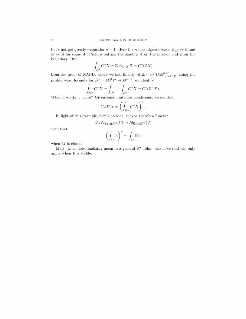
58 FACTORIZATION HOMOLOGY
Let’s not get greedy—consider n = 1. Here the n-disk algebra sends R≥0 7→ Z andR 7→ A for some A. Picture putting the algebra A on the interior and Z on theboundary. But ∫
D1
C∗X ' Z⊗C∗X Z ' C∗(ΩX)
from the proof of NAPD, where we had finality of ∆op → Disk∂,or1/[−1,1]. Using the
pushforward formula for Dn = (D1)n → Dn−1, we identify∫Dn
C∗X '∫D1
· · ·∫D1
C∗X ' C∗(ΩnX).
What if we do it again? Given some finiteness conditions, we see that
C∗ΩnX '
(∫Dn
C∗X
)∨.
In light of this example, here’s an idea: maybe there’s a functor
D : AlgDiskaugn
(V)→ AlgDiskaugn
(V)
such that (∫M
A
)∨'∫M
DA
when M is closed.Matt: what does dualizing mean in a general V? John: what I’ve said will only
apply when V is stable.

FACTORIZATION HOMOLOGY 59
24. Koszul duality [11/15/2017]
Koszul duality is something not about algebras, but about augmented algebras.
Definition 114. We say that A is an augmented k-algebra, for k commutative, ifwe are given a map A→ k of k-algebras.
In particular, the unit map composed with the augmentation k → A → k isnecessarily the identity map on k. If we now recall that a commutative algebra inV (symmetric monoidal) is equivalent to the data of a symmetric monoidal functor
FinA−→ V sending I 7→ A⊗I .
Definition 115. An augmented commutative algebra in V is a symmetric
monoidal functor Fin∗A−→ V (where the monoidal structure on finite pointed sets
is, if you like, the wedge product).
If we think of the algebra as the value of the functor A on 〈1〉∗, there is a mapA(〈1〉∗) → A(∗). This is exactly our classical augmentation. There is of course afunctor from Fin to Fin∗ so restriction along this functor is the forgetting of theaugmentation data. This yields the following definition.
Definition 116. An augmented n-disk algebra is a symmetric monoidal functor
Diskn,∗A−→ V.
Here the domain has objects∐
Rn t∗, and morphisms, away from the componentsthat they send to ∗, are embeddings. The symmetric monoidal structure is thewedge product.
Observe that an augmented commutative algebra yields an augmented n-diskalgebra, by the usual restriction.
Notice that there is a symmetric monoidal functor
Disk∂n → Diskn,∗
sending ∐I
Rn t∐J
Rn≥0 7→∐I
Rn t ∗.
From this observation we find that there is a restriction functor AlgaugDiskn
(V) →AlgDisk∂n
(V), which yields
Corollary 117. For A an augmented n-disk algebra, we can define∫M
A = colimDisk∂n/M
A
for M a manifold with boundary.
One might say that n-disk boundary algebras are more general, so why botherrestricting when working with manifolds with boundary? The reason is becauseKoszul duality applies to the augmented algebras.
Theorem 118. There exists a contravariant functor
AlgaugDiskn
(Ch)op AlgaugDiskn
(Ch)

60 FACTORIZATION HOMOLOGY
that on underlying objects assigns
A 7→(∫
DnA
)∨.
Here we are stating the theorem in minimal generality—what we need is that Vis stable.
Last time we saw that(∫Dn
C∗(ΩnX)
)∨' (C∗Mapsc(D
n, X))∨ ' C∗X.
Here C∗X is of course augmented. Given some (finiteness, etc.) conditions we alsosaw that (∫
DnC∗X
)∨' (C∗ΩnX)
∨ ' C∗ΩnX.
Exercise 119. Recall that if M is without boundary then we had∫M
Freen(V ) '∐i≥0
Confi(M)×Σi Vi
It is easy to see that the free n-disk algebra on the space V is augmented. Similarlyfor V ∈ (V,⊗), ∫
M
Freen(V ) '∐i≥0
Confi(M)Σi V⊗i.
For homework 14, allow M to have a boundary and let V = Ch. Show that∫M
Freen(V ) '⊕i≥0
Confi(M)/∂ Σi V⊗i.
Here Confi(M)/∂ is the subspace of Confi(M) such that at least one point liesin ∂M . Note also that is the tensor with pointed spaces. Then show that forM = Dn, ∫
DnFreen(V ) ' Z⊕ V [n].
Let me give you some hints. First note that the tensor X V ' C∗(X) ⊗ V isreduced chains. For i = 0 we get ∗Σ0 V
⊗0 = Z. For i = 1 we have
Conf1(Dn)/∂ Σ1V ' Dn/∂Dn V ' V [n]
since C∗(Sn) ⊗ V = Z[n]. What I’ve left for you for homework is to show that
Confi(Dn)/∂ ' ∗.
For future reference, what is the n-disk algebra structure on the dual of this?We have (∫
DnFreen(V )
)∨' Z⊕ V ∨[−n].
This is a general feature of Koszul duality—the dual of a free algebra is a trivialalgebra.
Add picture here

FACTORIZATION HOMOLOGY 61
25. The cotangent functor [11/20/2017]
Let’s think about one of the past homework problems together.
Lemma 120. We have that Confi(Dn)/∂ ' ∗ for i ≥ 2.
Proof. Note that for Nn−1 with ∂N = ∅ then
∂ Confk (N × [−1, 0))→ Confk(N × [−1, 0))
is a homotopy equivalence. We can do this by exhibiting a deformation retractionof this map. Let me sketch how this works for the circle (see sketch in notebook).Notice that this argument does not work for k = 0. In that case the right handside is a point and the left hand side is the empty set and there are no maps fromthe point to the empty set. Now notice that by translating the first point to thecenter Confi(D
n) ' Confi−1(Dn − 0) (can show this by replacing Dn with Rnand noting that Confi(Rn)→ Rn has the right fiber).
Okay, back to Koszul duality. It is in fact more general than just the form it takesfor n-disk algebras. Recall that the way we stated it we had a contravariant functor(∫Dn−)∨ : Algaug,op
n → Algaugn (abbreviating our notation of n-disk algebas). For
each n Koszul duality looks symmetric but in the limit where n→∞, the symmetryis broken:
Algcomm AlgLie
Algopn Algn
Algopn−1 Algn−1
T
C∗Lie
Let’s explain the maps at the very top, i.e. standard Koszul duality, in twoversions. In version 1, suppose we have some algebraic structure O such that thereis a trivial algebra functor
ChZ⊕−−−−→ AlgO(Ch).
This functor always preserves limits because it’s a right adjoint. More explicitly
given JA−→ AlgO(Ch)
fgt−→ Ch one shows that the limit of this composite functor hasan algebra structure. Have
lim fgt A⊗ lim fgt A lim fgt A
lim
(J × J (fgtA)⊗(fgtA)−−−−−−−−−−→ Ch
)which gives us what we want. This is all to say that there exists a left adjointfrom AlgO(Ch) → Ch, call it L for the “cotangent space” at the augmentation.
Big diagram hereHence we see that L FreeO is left adjoint to fgt triv = id, which implies thatL FreeO ' id. Observe now that L sends free algebras to what they are freeon L(FreeOV ) = V . Moreover L preserves colimits. Geometrically if you thinkof SpecA then the augmentation is a point A → Z and L is the cotangent spaceencoding infinitesimal data near the point.

62 FACTORIZATION HOMOLOGY
If O is the operad for commutative algebras then FreeO(V ) = Sym(V ) = O(AV )that is naturally augmented to Z. Then L(SymV ) = V is the usual Zariski cotan-gent space at 0.
Theorem 121. For A an n-disk algebra,
Z⊕ LA[n] '∫Dn
A.
I’ll maybe only sketch this proof (the details are in my Ph.D. thesis).
Proof sketch. We have already calculated that for A = Freen(V ),∫Dn
Freen(V ) ' Z⊕ V [n],
which followed from the fact that Confi(Dn)/∂ ' ∗ for i ≥ 2. On the other hand,
LFreen(V ) = V so ∫Dn
A ' Z⊕ LA[n].
for A free. Thus the two agree on free algebras.The next step is to show that∫
Dn− : Algaug
n (Ch)→ Ch
preserves homotopy colimits of ∆op-diagrams, i.e. for any
∆op A•−−→ Algaugn
∫Dn−−−→ Ch
there is always a map |∫Dn
A•| →∫Dn|A•| and this map is an equivalence. This
statement is a consequence of the fact that all reasonable functors (those appearingabove such as fgt and Free) preserve geometric realization. We have the iteratedfree forget simplicial resolution (monadic?) for A and this computes |Free•nA| whichtells us that∫
DnA '
∫Dn|Free•nA| ' |
∫Dn
Free•nA| ' |Z⊕ LFree•nA[n]| ' Z⊕ LA[n].
Since we have only a bit of time left let me give some intuition for why thegeometric realization is preserved.
Lemma 122. The functor ∆op → ∆op ×∆op is final (i.e. ∆op is “sifted”).
We don’t have time to prove this. Now consider the composite functor ∆op A•−−→Alg
fgt−→ Ch which we denote by A•. We produce a multiplication on |A•|. We have
∆op → ∆op ×∆op A×A−−−→ Ch× Ch⊗−→ Ch
sending n to An ⊗ An. Now colim(∆op → Ch) = |A ⊗ A| → |A•| By finality this
is equivalent to colim(∆op × ∆op A⊗A−−−→ Ch. But this map goes through Ch × Chvia tensor product. Since tensor product preserves colimits this is equivalent to
colim(∆op ∆−→ Ch)⊗ colimA.Grisha: can you do something similar for more general things like monads? John:
it’s not true in that level of generality as can be seen by the if and only if statementin the Bar-Beck theorem.

FACTORIZATION HOMOLOGY 63
26. Koszul duality II [11/27/2017]
Observe the following. For K a sifted category (nonempty with the diagonal
functor final), given a diagram K A−→ Alg(V)fgt−→ V. Then colim(K A−→ V) is an
algebra. This is because we have the composite
K → K×K A×A−−−→ V × V ⊗−→ Vand a natural transformation (via multiplication) from this composite to the functorA. Hence we obtain a map
colim(K → K×K → V)→ colim(K A−→ V).
By finality and the fact that the ⊗ in V preserves colimits, we obtain
colim(K ×K → V × V ⊗−→ V) ' ⊗ colim(K ×K → V × V) ' colim(K → V)⊗2.
Hence siftedness is important for preserving algebraic structures.The following more general result can be found in Lurie’s Higher Algebra, though
it is an older result.
Theorem 123. The forgetful functor fgt : AlgO(V⊗)→ V⊗ preserves sifted colimitsif ⊗ distributes over sifted colimits.
Lemma 124. The category ∆op is sifted.
We will need to recall how subdivision works for simplicial sets. Write nd[p]or the nondegenerate simplices of [p], which is the nerve of the poset ordered byinclusion. Clearly nd[0] = [0]. One checks that
nd[1] = 0 −→ 01←− 1.
For nd[2] one obtains the usual picture of the barycentric subdivision of the two-simplex. A little bit of work shows that we obtain a functor nd : ∆ → sSet. Wenow define the barycentric subdivision as the left Kan extension of nd:
∆ sSet
sSet
nd
In other words,sdX := colim
∆nd.
Lemma 125. For X a simplicial set, |X| ∼= |sdX|.
Proof sketch. I’ll leave the details for you, but the first case is when X = ∆[p].Then check that |∆[p]| = ∆p ∼= |nd[p]|. More generally, reduce |X| to each cell andapply the above logic.
Lemma 126. The diagonal functor ∆op → ∆op ×∆op is final.
Proof. We use Quillen’s theorem A and show that for any [p], [q], the classifyingspace
B(
∆op ×∆op×∆op (∆op ×∆op)[p]×[q]/)' ∗
is contractible. This is a bit clunky but we can rewrite as showing
B(∆/[p] ×∆ ∆/[q]
)=: B(∆/∆[p]×∆[q])
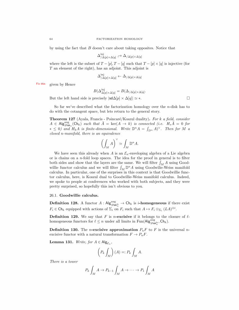
64 FACTORIZATION HOMOLOGY
by using the fact that B doesn’t care about taking opposites. Notice that
∆inj/∆[p]×∆[q] → ∆/∆[p]×∆[q]
where the left is the subset of T − [p], T − [q] such that T − [p]× [q] is injective (forT an element of the right), has an adjoint. This adjoint is
∆inj/∆[p]×∆[q] ← ∆/∆[p]×∆[q]
given byFix this Hence
B(∆inj∆[p]×∆[q] = B(∆/∆[p]×∆[q].
But the left hand side is precisely |sd∆[p]×∆[q]| ' ∗.
So far we’ve described what the factorization homology over the n-disk has todo with the cotangent space, but lets return to the general story.
Theorem 127 (Ayala, Francis - Poincare/Koszul duality). For k a field, considerA ∈ Algaug
D iskn(Chk) such that A = ker(A → k) is connected (i.e. H∗A = 0 for
∗ ≤ 0) and HkA is finite-dimensional. Write DnA =∫Dn
A)∨. Then for M aclosed n-manifold, there is an equivalence(∫
M
A
)∨'∫M
DnA.
We have seen this already when A is an En-enveloping algebra of a Lie algebraor is chains on a n-fold loop spaces. The idea for the proof in general is to filterboth sides and show that the layers are the same. We will filter
∫MA using Good-
willie functor calculus and we will filter∫M
DnA using Goodwilie-Weiss manifoldcalculus. In particular, one of the surprises in this context is that Goodwillie func-tor calculus, here, is Koszul dual to Goodwillie-Weiss manifold calculus. Indeed,we spoke to people at conferences who worked with both subjects, and they werepretty surprised, so hopefully this isn’t obvious to you.
26.1. Goodwillie calculus.
Definition 128. A functor A : Algaug
D iskfrn→ Chk is i-homogeneous if there exist
Fi ∈ Chk equipped with actions of Σi on Fi such that A 7→ Fi ⊗Σi (LA)⊗i.
Definition 129. We say that F is n-excisive if it belongs to the closure of `-homogeneous functors for ` ≤ n under all limits in Fun(Algaug
D iskfrn,Chk).
Definition 130. The n-excisive approximation PnF to F is the universal n-excisive functor with a natural transformation F → PnF .
Lemma 131. Write, for A ∈ AlgEn ,(Pk
∫M
)(A) =: Pk
∫M
A.
There is a tower
Pk
∫M
A→ Pk−1
∫M
A→ · · · → P1
∫M
A

FACTORIZATION HOMOLOGY 65
such that the fiber is given
C∗(Confk(M))⊗Σk (LA)⊗k Pk∫MA
k Pk−1
∫MA

66 FACTORIZATION HOMOLOGY
27. Manifold calculus [11/29/2017]
27.1. Goodwillie-Weiss manifold calculus. Last time we gave the quickest in-troduction to Goodwillie calculus known to mankind. Let’s now look at another“filtration”, the cardinality filtration.
Definition 132. Consider the category Disknun/M which has objects n-disks embed-
ding into M where the embeddings are surjections on π0. The morphisms are theπ0-surjective embeddings. The “nu” stands for nonunital, as algebras over this willno longer have units. This category is a (not full) ∞-subcategory of Diskn/M .
For the following it is important that our categories are ∞-categories and notjust posets.
Lemma 133. The map Disknun/M → Diskn/M is final.
Proof. Left as an exercise.
Define Disknu,≤in/M ⊂ Disknu
n/M to be the subcategory of n-disks that have |I| ≤ i
components. Then we define
τ≤i∫M
A = colim(Disknu,≤i
n/M → Chk).
Observe that since we can write Disknun/M = lim−→Disknu,≤i
n/M as a sequential colimit
and because colimits over colimits of categories are just iterated colimits (do thisabstract nonsense yourself, and note that it’s not true for limits), we find that∫
M
A = lim−→i
τ≤i∫M
A
via the above lemma.What are the layers in this filtration?
Lemma 134. For M closed, the following is a (homotopy) pushout:
τ≤i−1∫MA τ≤i
∫MA
k Confi(M)+ ⊗Σi A⊗i
Here we are taking the one-point compactification of the configuration space. If youlike, the bottom right can be written as twisted chains C∗(Confi(M)+
Σi, A⊗i)
Proof idea. We have already shown that Disknu,=in/M ' Confi(M)Σi . So what we
want to study is the quotient
Disknu,≤in/M /Disknu,≤i−1
n/M ' Confi(M)+Σi
and then apply some formal nonsense.
Proposition 135. For k⊕V a trivial En-algebra the cardinality filtration splits as∫M
k ⊕ V '⊕i≥0
Confi(M)+ ⊗Σi V⊗i.
FACTORIZATION HOMOLOGY 67
Compare this to the case of Goodwillie calculus for free algebras where we havea splitting ∫
M
FreeEn(W ) '⊕i≥0
Confi(M)⊗Σi W⊗i
which is quite similar. By Koszul duality,
Dn(FreeEnW ) '(∫
DnFreeEnW
)∨' (k ⊕W [n])∨ ' k ⊕W∨[−n].
Proposition 136. For A with connected augmentation ideal and H∗A finite rank,we have that (∫
M
A
)∨'∫M
DnA.
Proof. We will play this proof slightly fast and loose, for lack of time. SupposeA = FreeEnV . Then on the left we have(∫
M
FreeEnV
)∨=(⊕
Confi(M)⊗Σi V⊗i)∨
=∏i≥0
(Confi(M)⊗Σi V
⊗i)∨ .Observe now the following important fact. We always have a map ⊕i≥0Bi →∏i≥0Bi. This is an equivalence if Bi is (for simplicity) i-connective as i → ∞
(since finite sums and finite products are the same). Recall that V is 1-connective,whence V ⊗i is i-connective.2 Hence Confi(M)⊗V ⊗i is i-connective. Quotienting byΣi preserves this, as colimits preserve connectivity because we have an adjunction
Ch≥ik Chk.
left
τ≥i
Now the observation above allows us to simplify, up to equivalence, the directproduct to a direct sum: ⊕
i≥0
(Confi(M)⊗Σi V
⊗i)∨ .We want this to be the same as∫
M
Dn(FreeEnV ) '∫M
k ⊕ V ∨[−n] '⊕i≥0
Confi(M)+ ⊗Σi (V ∨[−n])⊗i
In particular we want(Confi(M)⊗Σi V
⊗i)∨ ' Confi(M)+ ⊗Σi (V ∨[−n])⊗i.
Let’s play with the left. The dual of a colimit is a limit so we have(Confi(M)⊗Σi V
⊗i)∨ ' (C∗(Confi(M))⊗Σi V⊗i)∨
'(C∗(Confi(M))∨ ⊗ (V ⊗i)∨
)Σi' C∗(Confi(M))∨ ⊗Σi (V ⊗i)∨
' C∗(Confi(M))⊗Σi (V ∨)⊗i
2Recall that the definition between connected and connective is just a shift.

68 FACTORIZATION HOMOLOGY
using the finiteness data that we have. On the right we have, playing a little loose(due to local coefficient issues)
C∗(Confi(M)+)⊗Σi (V ∨[−n])⊗i ∼ C∗Confi(M)+ ⊗Σi (V ∨)
⊗i[−ni]
∼ C∗ Confi(M)+ ⊗Σi (V ∨)⊗i
[−ni]using the norm map being an equivalence (since Confi(M) is a finite CW complexon which the symmetric group acts freely). Finally we apply usual Poincare duality,to obtain the left. This proves it for the free algebra.
For details, see AF’s paper Poincare/Koszul duality.
Grisha: is it obvious that the Goodwillie tower converges here? John: we needthe connectedness of the augmentation ideal. Otherwise the result is false. Thereis a more general result which is true, where Koszul dual of an algebra is a formalmoduli problem. There is a form of factorization homology that takes as input aformal moduli problem. In this case all the conditions may be removed. . . noticealso that here it was vital that we worked over a field so that we might swapconnectivity and coconnectivity.

FACTORIZATION HOMOLOGY 69
Appendix A. Exercises
Exercise 137. Construct homotopy equivalences
Emb(Rn,Rn) ' Diff(Rn) ' GL(n) ' O(n).
Exercise 138. Show that homotopy pullbacks are homotopy invariant.
Exercise 139. Show that compactly supported maps are covariant along openinclusions; in particular given an open inclusion U → V , the induced map of spacesMapsc(U,Z) → Mapsc(V,Z) is continuous. Here the topology on the mappingspaces is inherited from Maps∗(U
+, Z).
Exercise 140. Fill in the details of the proof that hocolim is homotopy invariant.
Exercise 141. Prove that there is a homeomorphism |∆[n]| ∼= ∆n. Moreover,show that the geometric realization |X| of a simplicial set X has the structure of aCW complex with an n-cell for each nondegenerate n-simplex.
Exercise 142. Show ∆[n]?∆[m] ∼= ∆[n+m+1] and the corresponding statementfor horns.
Exercise 143. Fill in the proof of Proposition 1.2.4.3 of HTT. In particular, showthat φ and ψ are indeed inverse.
Exercise 144. Prove that a localization C → D of ∞-categories are both initialand final.
Exercise 145. Show, for functors between ordinary categories, that a left Kanextension of a functor F : C → E along a functor g : C → D is given by the formula
g!F (d) = colimC/d
F.
70 FACTORIZATION HOMOLOGY
References
[AF15] David Ayala and John Francis. Factorization homology of topological manifolds. J. Topol.,8(4):1045–1084, 2015.
[Hir94] Morris W. Hirsch. Differential topology, volume 33 of Graduate Texts in Mathematics.
Springer-Verlag, New York, 1994. Corrected reprint of the 1976 original.[Lur09] Jacob Lurie. Higher topos theory, volume 170 of Annals of Mathematics Studies. Princeton
University Press, Princeton, NJ, 2009.


![DAVID AYALA & JOHN FRANCIS arXiv:1206.5522v5 [math.AT] 18 … · 2015. 8. 20. · arXiv:1206.5522v5 [math.AT] 18 Aug 2015 FACTORIZATION HOMOLOGY OF TOPOLOGICAL MANIFOLDS DAVID AYALA](https://static.fdocuments.in/doc/165x107/5fcf6fb9a33db1735f57c5c5/david-ayala-john-francis-arxiv12065522v5-mathat-18-2015-8-20-arxiv12065522v5.jpg)