Factor Timing with Cross- Sectional and Time-Series … · 30 FACTOR TIMING WITH CROSS-SECTIONAL...

30 FACTOR TIMING WITH CROSS-SECTIONAL AND TIME-SERIES PREDICTORS FALL 2017

PHILIP HODGES

is a managing director at BlackRock, Inc., in San Francisco, [email protected]

KED HOGAN

is a managing director at BlackRock, Inc., in San Francisco, [email protected]

JUSTIN R. PETERSON

is a vice president at BlackRock, Inc., in San Francisco, [email protected]

ANDREW ANG

is a managing director at BlackRock, Inc., in New York, [email protected]

Factor Timing with Cross-Sectional and Time-Series PredictorsPHILIP HODGES, KED HOGAN, JUSTIN R. PETERSON, AND ANDREW ANG

The premiums of factor strategies—often referred to as smart beta—incorporate two sources of pre-dict ability. First, well-known pat-

terns in the cross section at a point in time lead to long-run differences in portfolios with different characteristics; for example, stocks with high valuation ratios (value stocks) out-perform their peers with low valuation ratios (growth stocks). Second, the time series of portfolio returns of value stocks relative to growth stocks vary over time, and the expected return of one factor, such as value, also varies relative to other factor strate-gies, such as momentum. Further, the cross-sectional characteristics of factor strategies vary through time and are related to predictable components of factor returns.

In this article, we show how to com-bine both sources of cross-sectional and time-series information to predict smart beta returns—value, quality, size, momentum, and minimum-volatility strategies. Rather than present a comprehensive data mining exercise, we focus on a parsimonious set of predictors—all of which are economi-cally sensible. These predictors are known in the literature, and our contribution lies in showing how the predictive powers of the different signals compare to each other and how they can be combined.1 Our work builds on that of Asness et al. [2000], who examine valuation ratios of different factors

giving rise to “value of value” and “value of momentum” effects. The smart beta fac-tors also exhibit time-series momentum, as shown by Lewellen [2002], which we refer to as a relative strength indicator. We examine cross-sectional dispersion of signals similar to Cohen, Polk, and Vuolteenaho [2003].

We examine the behavior of factors across business and economic cycles—which has been well studied in the literature (see Ferson and Harvey [1991]). These patterns are intuitive: During economic troughs, value has tended to underperform because these companies have relatively inf lexible capital structures (Berk, Green, and Naik, [1999]), but minimum-volatility strategies have generally outperformed because of their risk mitigation properties (Ang et al. [2006]). As the economy has improved, momentum strategies have tended to do well. More defensive quality strategies, as well as minimum-volatility strategies, have generally come into favor at the top of the economic cycle as the pace of economic growth slows and the probability of a recession increases.

We show how to combine the cross-sectional signals with the time-series, business cycle regimes. In particular, we show how the business cycle information can be incorporated as a cross-sectional signal and then combined bottom up with the other cross-sectional sig-nals. Taken alone, the signal with the best predictive results comes from positioning across

JPM-Hodges.indd 30JPM-Hodges.indd 30 04/10/17 5:45 pm04/10/17 5:45 pm

IT IS IL

LEGAL TO REPRODUCE THIS A

RTICLE IN

ANY FORMAT

THE JOURNAL OF PORTFOLIO MANAGEMENT 31FALL 2017

the business cycle. An important result is that reliance on only one predictor—such as valuation indicators, as in Arnott et al. [2016]—leads to significantly inferior results compared to using combinations of several signals.

Finally, we show that timing style factors with valuation and relative strength signals does not result in persistent tilts to value or momentum style factor exposures. We examine position data of the style factor portfolios resulting from the individual factor timing strategies and show that time variation in the cross-sectional holdings does not permanently lean into certain factors. Put another way, using valuation as a timing signal does not result in persistent overweights to a value factor.

DATA AND METHODOLOGY

We use a variety of data sources. The factors them-selves are represented by third-party smart beta indices. The predictive signals are constructed using information from several databases and include both stock-specific and macroeconomic data.

Smart Beta Strategies

We take MSCI smart beta indices as our defini-tions for the factors: value, quality, momentum, size, and minimum volatility.2 This implementation of factor investing, computed independently by a third-party index provider, is long only and fully transparent, and can be directly traded by individuals with exchange-traded funds (ETFs).3 We, like others in the industry, refer to factor investing done through long-only ETFs as “smart beta.” We note that the ability to directly trade these vehicles makes them an option for use in model portfolios or for individual investors to use as active strategies or overlays. We focus on the predictive signals themselves, setting aside the exercise of creating highly optimized portfolios based upon those signals.

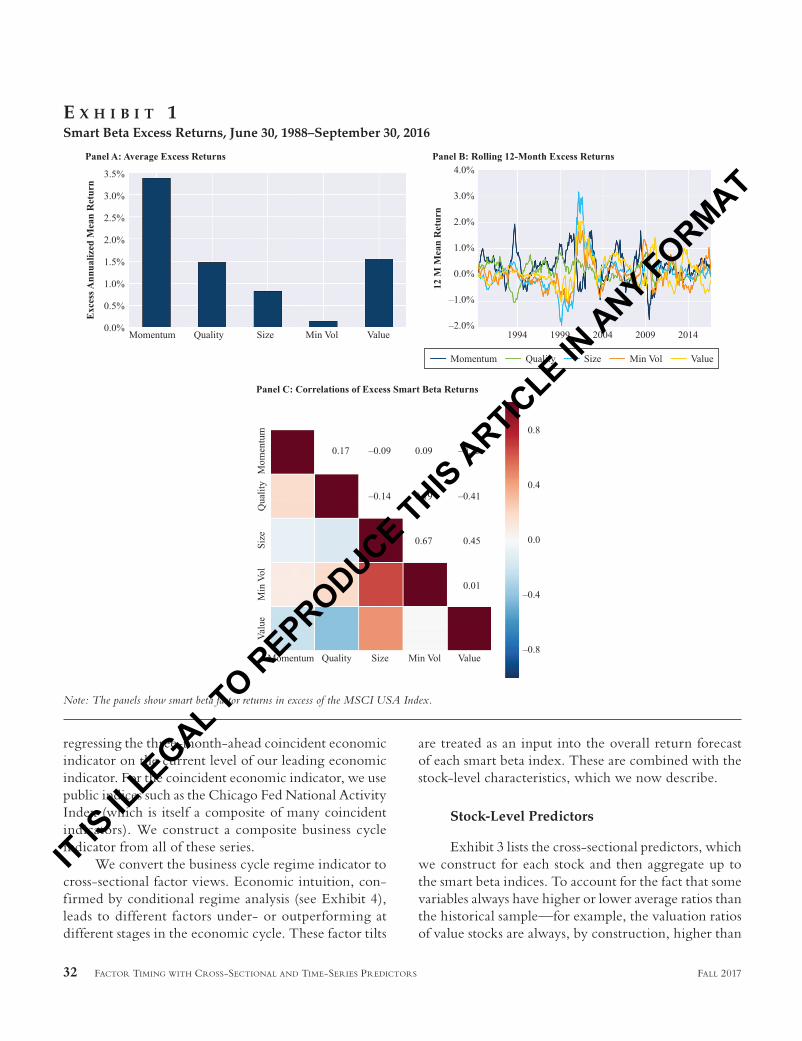
Exhibit 1, Panel A, plots the average excess returns (in excess of the MSCI USA Index) of each smart beta factor from June 30, 1988, to September 30, 2016. The average returns of value, quality, momentum, and size are positive: momentum and value have experienced the highest excess returns of 3.4% and 1.5% per year, respectively. Minimum volatility has experienced an average return in line with the market (with less risk), consistent with the findings of Ang et al. [2006].

Exhibit 1, Panel B, graphs 12-month moving averages of the excess factor returns and shows that while the long-run excess premiums are positive, there is pro-nounced time variation across the sample. For example, size switches from a negative 12-month mean return of −2.0% in 1999 to 3.0% in the early 2000s. Panel C shows that the excess factor returns are not highly correlated: The lowest correlation is between value and quality at −0.42, while the highest correlation of 0.67 is between minimum volatility and size. Note that momentum and value are negatively correlated with a correlation of −0.22, which is consistent with the well-known negative relationship between these two factors (see Asness et al. [2013]).

The use of third-party indices for factor returns has the advantage that our style factors may be investable via ETFs designed to track the corresponding indices. Addi-tionally, we take advantage of the complete transparency of holdings data to construct stock-level characteristics of each portfolio. Importantly, the smart beta indices have independent construction rules that do not incorporate timing information. That is, the factors embed certain cross-sectional information that gives rise to uncondi-tional excess returns. The cross-sectional signals we use to predict conditional factor performance and time factors are distinct from those signals directly used to construct each factor. Thus, our timing results are additive to the excess returns generated by static factor strategies.

Business Cycle Indicator

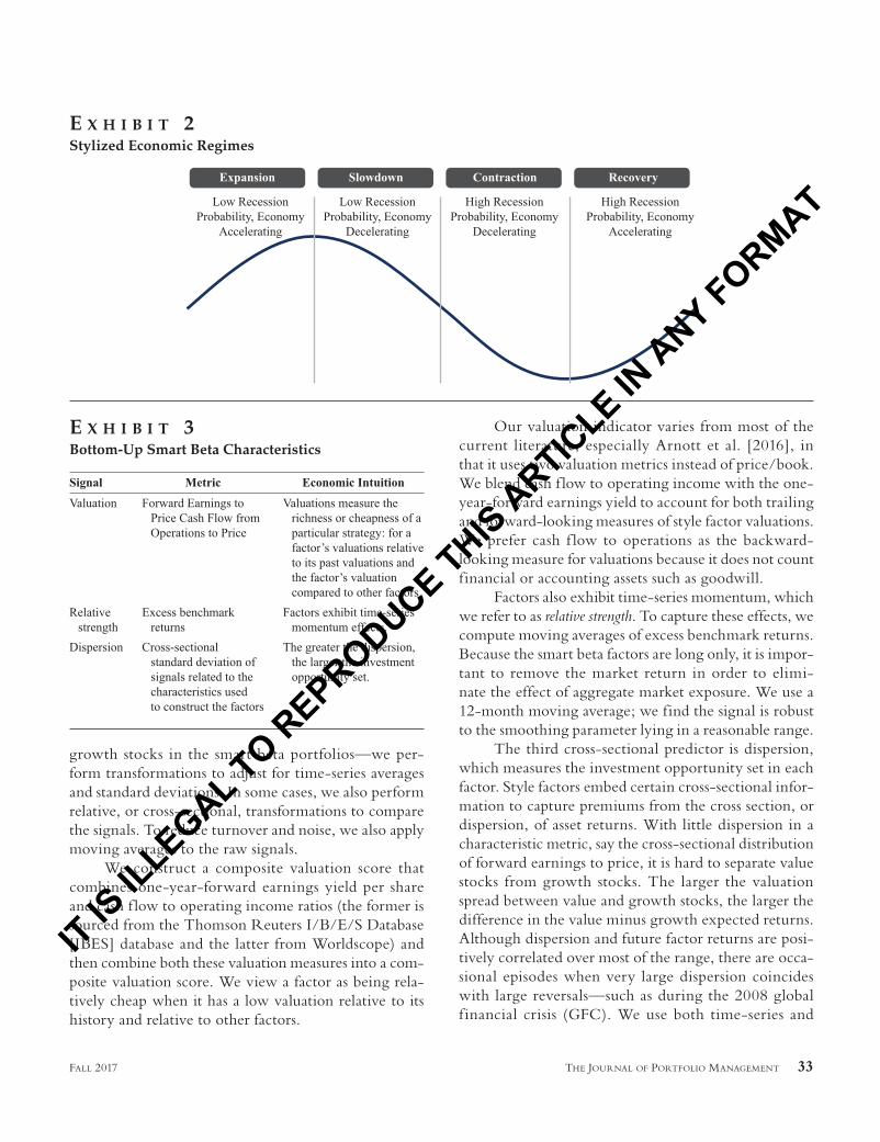
We use various leading and coincident indicators to model the economic cycle.4 We identify four regimes: expansion, slowdown, contraction, and recovery. Exhibit 2 illustrates this stylized business cycle. We first determine if the rate of economic change is positive or negative by measuring the change in our leading economic indicators, which includes measures such as the Citi U.S. Leading Indicator for Consensus Economic Forecasts and forecasts from Consensus Economics. We define acceleration as increases in growth in excess of one standard deviation. Similarly, we define deceleration as decreases in growth below a negative one standard deviation. Observations that fall between plus and minus one standard deviation thresholds are set to the previous period’s classification.

We further subdivide states of the economy based on whether there is a high or low probability of entering into a recession. More specif ically, we forecast the likelihood of a recession in the subsequent period by


IT IS IL


RTICLE IN

ANY FORMAT


regressing the three-month-ahead coincident economic indicator on the current level of our leading economic indicator. For the coincident economic indicator, we use public indices such as the Chicago Fed National Activity Index (which is itself a composite of many coincident indicators). We construct a composite business cycle indicator from all of these series.

We convert the business cycle regime indicator to cross-sectional factor views. Economic intuition, con-firmed by conditional regime analysis (see Exhibit 4), leads to different factors under- or outperforming at different stages in the economic cycle. These factor tilts

are treated as an input into the overall return forecast of each smart beta index. These are combined with the stock-level characteristics, which we now describe.

Stock-Level Predictors

Exhibit 3 lists the cross-sectional predictors, which we construct for each stock and then aggregate up to the smart beta indices. To account for the fact that some variables always have higher or lower average ratios than the historical sample—for example, the valuation ratios of value stocks are always, by construction, higher than

E X H I B I T 1Smart Beta Excess Returns, June 30, 1988–September 30, 2016

Note: The panels show smart beta factor returns in excess of the MSCI USA Index.


IT IS IL


RTICLE IN

ANY FORMAT


growth stocks in the smart beta portfolios—we per-form transformations to adjust for time-series averages and standard deviations. In some cases, we also perform relative, or cross-sectional, transformations to compare the signals. To reduce turnover and noise, we also apply moving averages to the raw signals.

We construct a composite valuation score that combines one-year-forward earnings yield per share and cash f low to operating income ratios (the former is sourced from the Thomson Reuters I/B/E/S Database [IBES] database and the latter from Worldscope) and then combine both these valuation measures into a com-posite valuation score. We view a factor as being rela-tively cheap when it has a low valuation relative to its history and relative to other factors.

Our valuation indicator varies from most of the current literature, especially Arnott et al. [2016], in that it uses two valuation metrics instead of price/book. We blend cash f low to operating income with the one-year-forward earnings yield to account for both trailing and forward-looking measures of style factor valuations. We prefer cash f low to operations as the backward-looking measure for valuations because it does not count financial or accounting assets such as goodwill.

Factors also exhibit time-series momentum, which we refer to as relative strength. To capture these effects, we compute moving averages of excess benchmark returns. Because the smart beta factors are long only, it is impor-tant to remove the market return in order to elimi-nate the effect of aggregate market exposure. We use a 12-month moving average; we find the signal is robust to the smoothing parameter lying in a reasonable range.

The third cross-sectional predictor is dispersion, which measures the investment opportunity set in each factor. Style factors embed certain cross-sectional infor-mation to capture premiums from the cross section, or dispersion, of asset returns. With little dispersion in a characteristic metric, say the cross-sectional distribution of forward earnings to price, it is hard to separate value stocks from growth stocks. The larger the valuation spread between value and growth stocks, the larger the difference in the value minus growth expected returns. Although dispersion and future factor returns are posi-tively correlated over most of the range, there are occa-sional episodes when very large dispersion coincides with large reversals—such as during the 2008 global f inancial crisis (GFC). We use both time-series and

E X H I B I T 2Stylized Economic Regimes

E X H I B I T 3Bottom-Up Smart Beta Characteristics


IT IS IL


RTICLE IN

ANY FORMAT


cross-sectional normalizations to account for the fact that the mean dispersion varies by style factor. That is, the average dispersion in the value factor will be dif-ferent from the average dispersion in the minimum-volatility factor.

We aggregate each of these stock-level predic-tors to the smart beta portfolio level and then combine each predictor to come up with an aggregate view on each factor. In doing so, we do not further optimize the different weights of the signals. This is because Smith and Wallis [2009], among others, find that estimating weights in forecast combinations often introduces noise and reduces out-of-sample performance. Thus, we simply combine each predictor with equal weights. We use a risk model for the optimization to convert the return forecasts into holdings. The risk model is based on a covariance matrix estimator of the smart beta index returns in excess of cash.

EMPIRICAL RESULTS

In this section, we report the efficacy of the smart beta predictors concentrating on the risk–return perfor-mance of tradeable factor portfolios. Our main takeaway is that forecast combinations have greater predictive power than any single predictor. This is consistent with the large statistical literature begun by Bates and Granger [1969] documenting the superior out-of-sample forecasts produced by combinations of predictors. On a stand-alone basis, the business cycle indicator has produced the best outperformance.

Factors Across the Business Cycle

Exhibit 4 reports the business cycle regimes we estimate from December 1984 to September 2016. The regimes accord with economic intuition, and some align with those identified from the National Bureau of Economic Research (which are identif ied ex post and sometimes well after the fact). In Exhibit 4, we plot the quarterly annualized real growth rate for the United States. The color of the observations correspond to one of the four economic environments of our regime model.

Exhibit 4 illustrates the slowdown and then the recovery during the early 1990s, and the largely expan-sionary period, punctuated with some mild slowdowns during the mid- to late-1990s. There is a marked

slowdown during the early 2000s that we mostly classify as a contraction. The business cycle indicator is positive, cycling between expansion and slowdown from 2001 to 2007, when it begins a steep contraction coinciding with the GFC. Since 2010, the economy cycled between expansion and slowdown stages at the high point of the business cycle. This is not unusual: Our model suggests that an economy in slowdown is approximately three times more likely to shift back into expansion than to slip into contraction.

In Exhibit 4, Panel B, we report excess returns of the best-performing smart beta indices conditional on each regime. During expansions when the economy has well-established trends, momentum has tended to do well: This is demonstrated by momentum having a Sharpe ratio of 0.80 in this regime. Minimum volatility and quality have tended to outperform at the peak of the business cycle, which is when the economy starts to turn, with Sharpe ratios of 0.25 and 1.50, respectively. During these regimes, the economy is exposed to addi-tional shocks; we prefer safety strategies designed to mitigate risk and strategies favoring companies with lower leverage and more steady earnings. We find that during contraction regimes, all the factors have tended to modestly outperform the market, but the biggest differentiation is the relative underperformance of momentum. Finally, when the economy recovers from its trough, size and value have been the best-performing factors with Sharpe ratios of 2.55 and 2.95, respectively.

Timing Factors with Business Cycle Indicators

We use the economic regime indicator in a factor timing strategy as follows. First, we estimate which regime prevails at each point in time. Using a cross-sectional normalization, we assign positive weight to those factors that have tended to outperform according to the stage of the business cycle the economy is in, as identified in Exhibit 4, Panel B. We also cross-sectionally penalize the smart beta factors that underperform during that prevailing regime. The output of this processing is a long–short factor portfolio that incorporates the conditional information assigned to the current market regime. We target a 1% risk level in the strategy.

Exhibit 5 examines the performance of timing the smart beta factors using the economic regime infor-mation. We graph cumulated excess log returns of the


IT IS IL


RTICLE IN

ANY FORMAT


timing strategy based on economic regime information. The signal has strong performance during the begin-ning and latter portion of the sample from September 1992 to March 2000 and from July 2008 to September 2016, respectively. Over the whole sample, the economic regime indicator generated a Sharpe ratio of 0.71. The signal had a period of weak performance from October 2003 to July 2008; this period also coincided with its largest drawdown of 1.6%.

Exhibit 5 shows that the economic regime indi-cator correctly positioned the portfolio coming into the recession of July 1990 to March 1991—generating posi-tive returns from being overweight to momentum prior to the summer of the 1990 before switching into defen-sive positioning, being long minimum volatility and quality through the recession. The signal had its stron-gest performance from January 1997 through June 2002. As the economy oscillated between expansion and

E X H I B I T 4Business Cycle Signals


IT IS IL


RTICLE IN

ANY FORMAT


slowdown, the signal benefited from overweight posi-tions to momentum and an underweight to minimum volatility, with the exception of the period of the dot-com bubble when the signal correctly transitioned to a defensive portfolio as the economy slowed.

The indicator’s worst performance was from October 2003 through July 2008. This period was characterized by an economy that oscillated between expansions and slowdown. The relatively fast transitions were not captured well by the factor positions implied by the economic signal. As the economy slowed prior to the GFC in 2008, the economic regime indicator transitioned to a defensive portfolio generating positive returns over the period.

Stand-Alone Factor Timing Predictors

In Exhibit 6, Panel A, we report performance statistics of timing portfolios for each individual factor timing predictor. For completeness, the business cycle

signal in the first row corresponds to the factor timing of the economic regime indicator whose cumulated returns are graphed in Exhibit 5. All the strategies are constructed to target 1% risk. The average Sharpe ratio across all the predictors is 0.42 over the simulation period, with the highest Sharpe ratio resulting from the business cycle indicator. The weakest stand-alone timing predictor is dispersion, which has a Sharpe ratio of 0.38 over the sample period.

The last column of Panel A reports the drawdown period of each predictor; they are not the same, which points to the diversification potential in combining the different predictors. This diversification is illustrated in Panel B, which reports the correlations of the returns of each factor timing strategy. Note that the timing strategy based on relative strength has negative correlations of −0.20 and −0.31 between the valuation and dispersion indicators, respectively. The economic regime indicator is positively correlated with relative strength (correlation of 0.40), but negatively correlated with valuation and

E X H I B I T 5Performance of Timing Factors with the Business Cycle Indicator


IT IS IL


RTICLE IN

ANY FORMAT


dispersion indicators at −0.27 and −0.32, respectively. Thus, we expect that there should be diversif ication benefits to combining the predictors—which we show in the section on combining indicators.

In Exhibit 6, Panel C, we show the relative per-formance of each stand-alone factor timing predictor categorized by calendar year and ranked in descending order by Sharpe ratio. In this panel, the horizontal line represents a Sharpe ratio of zero, which acts as a bench-mark for the long–short factor predictors. The average positive returns of the predictors are apparent because the majority of their yearly returns are positioned above the zero threshold. Exhibit 6 also shows the diversi-f ication benefits of using multiple indicators by the changing best- and worst-performing factor timing indicators from year to year.

Relative strength. The relative strength indicator picks up the trends in each factor and overweights the factors with recent high performance and underweights those with recent low performance. The average holdings of the style factors in this indicator are, therefore, a function of the moving-average returns of the factors, as shown in Exhibit 1, Panel A.

The relative strength strategy generates a Sharpe ratio of 0.42 over the sample. The signal was able to iden-tify the trends in the factor returns in the mid-2000s, which ref lect the underlying positive economic trends over this period. After the GFC, there was short-term mean reversion in factor performance, which led to the relative strength strategy underperforming over this time. In the latter part of the sample from 2013 to 2015 when consistent trends in the market were reestablished, the indicator generated positive performance.

Valuations. The valuations predictor has an overall Sharpe ratio of 0.48. The majority of the gains, however, come from periods following market extremes. In some periods, a factor’s valuation can dominate the cross-sectional dimension on which the style factor is constructed. For example, during the f light-to-quality episode of the 2008 GFC, momentum and minimum volatility began to look very expensive by historical standards, whereas the value style factor began to look very cheap.5 In the aftermath of the GFC, as markets recovered, the valuations indicator generated strong returns due to long positioning in the value factor and short positioning in minimum-volatility and momentum factors. We observed similar dynamics in the period after the dot-com bubble in the early 2000s.

Dispersion. On a stand-alone basis, the dispersion indicator is the weakest of the predictors we consider. We find that dispersion has the strongest predictive power for factors constructed along a fundamental metric such as value and quality. During the 2008 GFC, the indi-cator was positioned to be underweight minimum vola-tility and size, and long value and momentum. In this period, the f light-to-quality characteristics of minimum volatility outweighed its weak dispersion characteristics, leading to losses in the dispersion strategy during this time. Despite the weaker performance of this predictor, the correlation properties—negative correlation with the relative strength predictor and mildly positive cor-relation with the valuation predictor—make the signal valuable when combined with others.

Styles of Styles

Value and momentum are factor portfolios, but valuation and relative strength are also used to time those factors. That is, we use similar metrics in the construc-tion of the factors to time those factors. Does this per-haps lead to “double counting” or “doubling down” on value or momentum?

To examine this question, we compare the asset-level positions resulting from each timing strategy, aggregating across the smart beta indices with the cor-responding value or momentum factors. We explain this analysis using the valuations indicator as follows. First, the timing strategy gives a set of weights for each of the smart beta indices. Second, we calculate the asset-level positions as the summation of the smart beta index active holdings multiplied by their respective smart beta index weights. Then we measure the cross-sectional holdings correlation of the valuation indicator’s asset-level active positions with the active positions of the value style factor index. We repeat this for each month in our simulation. To construct the holdings-level analysis for the relative strength indicator, we follow the same steps but use the relative strength smart beta index weights to calculate the asset-level positons and the momentum factor for measuring the cross-sectional holdings correlation.

Exhibit 7 reports the results. Panel A shows that the cross-sectional holdings of the valuation timing strategy have, on average, a correlation close to zero with the value factor. The correlation is positive or negative at different points in time. Thus, the valu-ation indicator is acting as a conditioner on portfolio


IT IS IL


RTICLE IN

ANY FORMAT


positioning, rather than an explicit and persistent increase in exposure to the value style factor. We also report the cross-sectional holdings correlation of a static strategic portfolio (i.e., an equal-weighted portfolio of each of the factors) with the value factor. As expected, that correlation is positive and varies slowly over time because the value factor has a constant weight in the strategic portfolio. (It is not constant because the con-stituents of each factor change over time and the indi-vidual factors are rebalanced.)

Panel B repeats the exercise for the relative strength timing strategy: It reports holdings-level correlations of the portfolio positions resulting from using the rela-tive strength indicator with the momentum factor. Again, the time variation in the cross-sectional holdings is centered around zero, and the relative strength indi-cator acts to condition the loading on the momentum style factor. In both examples, we see time variation in the cross-sectional holdings correlation that does not simply “load up” on each respective style factor.

Combining Factor Timing Indicators

Exhibit 8 reports the performance of combining all the indicators into an aggregate indicator. The com-bined return series begins in January 1990 with the relative strength and regime indicators. In December 1999, we add the valuation and dispersion indicators. To combine the indicators, we scale each individual indicator portfolio to 1% ex ante risk and then blend the holdings with equal weight to each of the four indica-tors. Because of the diversification of the predictor set, the resulting risk is below 1%, so we scale portfolio risk to a 1% risk target a second time. This transformation allows us to compare the predictability of the combined signal with those of the stand-alone ones.

Exhibit 8, Panel A, reports summary statistics for the combined model. The Sharpe ratio of the combined strategy is 0.88, which is higher than the Sharpe ratios of any individual stand-alone strategies (see Exhibit 6). This ref lects the diversification benefits from blending positive factor predictors with mildly positive and

E X H I B I T 6Timing Smart Beta Factors

(continued)


IT IS IL


RTICLE IN

ANY FORMAT


EX

HI

BI

T 6

(con

tinue

d)T

imin

g S

mar

t Bet

a Fa

ctor

s


IT IS IL


RTICLE IN

ANY FORMAT


negative correlations. The diversif ication benefits are also evident in a smaller maximum drawdown of the aggregate signal compared to the average maximum drawdown of each indicator.

Although we provide examples of both the con-tinuous and discrete diversif ication benef its of the multiple indicator approach, the GFC provides a spe-cific case study to showcase the merits of the aggregate indicator set. The relative strength indicator generated positive returns during the GFC because of overweights in quality and minimum volatility, while the valuation indicator underperformed during the same period. Post-GFC, the performance of the two indicators reversed as the relative strength indicator underperformed, and the valuation indicator performed strongly because of

short positions in the momentum style factor and a long position in the value style factor. The net positioning resulted in positive performance through the duration of the GFC. By construction, the aggregate model benefits from insights that incorporate both the recent perfor-mance and current valuations while being additive to the strategic allocation of style factors.

In Exhibit 8, Panel B, we demonstrate the addi-tivity of the factor timing model to a strategic smart beta portfolio of equally weighted factor positions. The figure shows the cumulative log return of the combined factor timing model when combined with a strategic smart beta allocation. In this analysis, the factor timing model is scaled to 2% ex ante risk prior to blending with the strategic allocation.6 The combined portfolio

E X H I B I T 7Styles of Styles


IT IS IL


RTICLE IN

ANY FORMAT


E X H I B I T 8Aggregate Smart Beta Timing Model


IT IS IL


RTICLE IN

ANY FORMAT


is generated by adding the strategic allocation holdings with the long–short portfolio generated from the factor timing model. In addition to the positive incremental returns, the factor timing model returns have a very low correlation of 0.09 with the strategic smart beta portfolio.

In Panel C, we conduct a similar analysis, but this time in style factor space by removing the market return from the strategic portfolio. (A practical implementation of this strategy requires taking short positions in factor ETFs.) Similar to Panel B, the inclusion of the factor timing indicator results in improved performance com-pared to the strategic style factor allocation. The composite factor timing model has returns that are −0.01 correlated with the strategic style factor strategic allocation.

CONCLUSION

We show that there is greater predictive power in tactically allocating among factor strategies by combining information from several predictors rather than using indi-vidual predictors. In particular, we show that constructing an aggregate indicator from economic regime, valuation, relative strength, and dispersion indicators produces better results than using those predictors on a stand-alone basis. We also show that using valuation and relative strength indicators to time smart beta factors has not resulted in persistent tilts to value or momentum factors, respectively.

The usual caveats apply to our work, including (1) the predictors we use are already known in the litera-ture and so there is a selection bias, (2) the portfolios are theoretical and there may be additional costs in imple-mentation, and (3) the simulations require estimates of model inputs for optimization. Nevertheless, the framework using position-level characteristics to time factor portfolios can potentially be extended to other predictors. In particular, though our work has concen-trated on timing long-only smart beta factors, the same methodology can be applied for long–short factors, as well as factors in other asset classes.

A P P E N D I X

Smart Beta Factors

Definitions. (Source: MSCI).7

Momentum (USA Momentum Standard) measures the performance of U.S. mid- and large-capitalization stocks exhibiting relatively higher price momentum characteristics,

while maintaining reasonably high trading liquidity, invest-ment capacity, and moderate turnover.

Quality (USA Quality Standard) measures the performance of U.S. mid- and large-capitalization stocks as identif ied through three fundamental variables: return on equity, earnings variability, and debt/equity.

Value (USA Value-Weighted Standard) measures the performance of U.S. mid- and large-capitalization stocks with value characteristics (book value/price, 12-month for-ward earnings/price, and dividend yield).

Size (USA Risk-Weighted Standard) measures the performance of U.S. mid- and large-capitalization stocks with a tilt toward the smaller, lower risk stocks within that universe.

Minimum Volatility (USA Minimum-Volatility Standard) measures the performance of U.S. mid- and large-capitalization stocks that, in the aggregate, have lower vola-tility characteristics relative to the broader U.S. equity market.

ENDNOTES

This material is not intended to be relied upon as a forecast, research, or investment advice, and is not a recom-mendation, offer, or solicitation to buy or sell any securities or to adopt any investment strategy. The information and opinions contained in this material are derived from proprie-tary and nonproprietary sources deemed by the authors to be reliable, are not necessarily all-inclusive, are not guaranteed as to accuracy, and may change as subsequent conditions vary.

The views expressed here are those of the authors alone and not of BlackRock, Inc. We thank Debarshi Basu, Ted Daverman, Garth Flannery, Michael Gates, He Ren, and Sara Shores for helpful comments.

1There is a large amount of literature, which cannot be done justice here. Ang [2014] provides a summary of some developments in the literature on time-varying factor returns.

E X H I B I T A 1Smart Beta Factors and Related Index

aPrior to November 30, 1997, the exposure is represented by the MSCI USA Quality Gross Index.bPrior to November 30, 1998, the exposure is represented by the MSCI USA Value Weighted Index.


IT IS IL


RTICLE IN

ANY FORMAT


2Further index details are in the appendix.3The expense ratios of the investable ETFs corre-

sponding to these indices are not taken into account in the performance of the MSCI indices. Because we represent the factor premiums using long-only MSCI indices, we use the terms “smart beta” and “factor investing” interchange-ably in this article.

4There is extensive literature on defining which eco-nomic data series lead or are coincident with the business cycle (see, for example, Zarnowitz [1992]).

5Momentum appeared expensive by historical stan-dards, based on the relatively long period of poor market performance relative to the length of the formation window. Minimum volatility became expensive because the price of low-risk stocks was bid up as investors searched for safety in their portfolios.

6This risk level is also consistent with a potential long-only implementation of the factor timing in which explicit shorting is not allowed.

7See index factsheets at https://www.msci.com/msci-factor-indexes.

REFERENCES

Ang, A. Asset Management: A Systematic Approach to Factor Based Investing. New York, NY: Oxford University Press, 2014.

Ang, A., R.J. Hodrick, Y. Xing, and X. Zhang. “The Cross-Section of Volatility and Expected Returns.” The Journal of Finance, Vol. 61, No. 1 (2006), pp. 259-299.

Arnott, R., N. Beck, V. Kalesnik, and J. West, “How Can ‘Smart Beta’ Go Horribly Wrong?” Fundamentals, Research Affiliates, 2016.

Asness, C., J.A. Friedman, R.J. Krail, and J.M. Liew. “Style Timing: Value versus Growth.” The Journal of Portfolio Management, Vol. 26, No. 3 (2000), pp. 50-60.

Asness, C., T.J. Moskowitz, and L.H. Pedersen. “Value and Momentum Everywhere.” The Journal of Finance, Vol. 68, No. 3 (2013), pp. 929-985.

Bates, J.M., and C.W. Granger. “The Combination of Forecasts.” Journal of the Operational Research Society, Vol. 20, No. 4 (1969), pp. 451-468.

Berk, J.B., R.C. Green, and V. Naik. “Optimal Investment, Growth Options, and Security Returns.” The Journal of Finance, Vol. 54, No. 5 (1999), pp. 1553-1607.

Cohen, R.B., C. Polk, and T. Vuolteenaho. “The Value Spread.” The Journal of Finance, Vol. 58, No. 2 (2003), pp. 609-642.

Ferson, W.E., and C.R. Harvey. “The Variation of Economic Risk Premiums.” Journal of Political Economy, (1991), pp. 385-415.

Lewellen, J. “Momentum and Autocorrelation in Stock Returns.” The Review of Financial Studies, Vol. 15, No. 2 (2002), pp. 533-564.

Smith, J., and K.F. Wallis. “A Simple Explanation of the Fore-cast Combination Puzzle.” Oxford Bulletin of Economics and Statistics, Vol. 71, No. 3 (2009), pp. 331-355.

Zarnowitz, V. “Composite Indexes of Leading, Coincident, and Lagging Indicators.” In Business Cycles: Theory, History, Indicators, and Forecasting, pp. 316-356. Chicago: University of Chicago Press, 1992.

To order reprints of this article, please contact David Rowe at [email protected] or 212-224-3045.


IT IS IL


RTICLE IN

ANY FORMAT

Factor Timing with Cross- Sectional and Time-Series … · 30 FACTOR TIMING WITH CROSS-SECTIONAL...

Documents

Transcript of Factor Timing with Cross- Sectional and Time-Series … · 30 FACTOR TIMING WITH CROSS-SECTIONAL...