1

MINISTRY OF FINANCE, GOVERNMENT OF INDIA

Working Paper No.3 /2009-DEA

Factor Employment, Sources and Sustainability of Output

Growth: Analysis of Indian Manufacturing

Arvind Virmani and Danish A. Hashim

April, 2009

2

The Economic Division in the Department of Economic Affairs has initiated a Working Paper series with the objective of improving economic analysis and promoting evidence based policy formulation in its mandated areas of work. The themes to be covered in the series include macro-economic and sectoral issues of relevance for national policy, strategy for addressing emerging global and national development concerns and the agenda for economic policy reforms. While the issues identified for the Working Papers have relevance as inputs for the flagship publication of the Department, namely Economic Survey and the Mid-Year Review, issues that are related to the larger work responsibility of the Department of Economic Affairs, including the economic aspects of financial services, revenues and expenditure are also the subject matter of this initiative. Papers prepared by the staff or commissioned by the Economic Division as well as other Divisions in the DEA will be included in the Working Paper series on suitable peer review.

3

Factor employment, Sources and Sustainability of output growth: Analysis of Indian Manufacturing1

Arvind Virmani2 and Danish A. Hashim3

1 The initial research, on which this study is based, was carried out by the authors when they were at the Indian Council for Research on International Relations (ICRIER). Authors are grateful to B.N. Goldar, Arup Mitra and D. N. Nayak for their valuable comments and suggestions. The usual disclaimer nevertheless applies. 2Economic Division, Department of Economic Affairs, Ministry of Finance, Government of India. 3 Research & Advocacy, Financial Technologies (India) Limited (FTIL).

The Working Paper does not in any way represent the views of the Ministry of Finance, Government of India. The views expressed in this paper are strictly those of the authors and not necessarily of the organisations authors belong to.

4

Contents

Abstract----------------------------------------------------------------------------------i

1. Introduction---------------------------------------------------------------------------- 2 Literature Review---------------------------------------------------------------------------

3 Methodology ----------------------------------------------------------------------------------- 4 Data and Variables---------------------------------------------------------------------------- 5 Empirical Findings--------------------------------------------------------------------------------- 6 Summary and Conclusion-----------------------------------------------------------

References---------------------------------------------------------------------------------------------------

Appendix-------------------------------------------------------------------------------------------------

List of Tables

Table1: Augmented Dickey-Fuller Test of Stationarity---------------------------------------- Table 2: Johansen Cointegration Test----------------------------------------------------------- Table 3: Trends in Select Indicators-------------------------------------------------------------- Table 4: Growth Rates of Select Indicators (%)------------------------------------------------ Table 5: Marginal Productivity and Price of Factor-------------------------------------------- Table 6: Decomposition of the growth in employment and share of labour (in %)------- Table 7: Decomposition of the growth in deployment and share of capital---------------- Table 8: Contributory factors to the output growth (in %)------------------------------

List of Figures

Figure 1: Trends in Select Variables------------------------------------------------------------- Figure 2: Trends in marginal productivity of labour and its wage rate---------------------- Figure 3: Trends in marginal productivity of capital and its price---------------------------

Tables of Appendix

Table A1: Pair wise Granger Causality Tests (1973-2001)------------------------------------ Table A2: Production Structure of Aggregate Manufacturing (1973-2001): Single Equation Estimates---------------------------------------------------------------------------------------------- Table A3: SURE Estimates of Growth Equations of Productivity (1973-2001)-------------- Table A4: Decomposition of the Growth in Employment and Share of Labour through Growth Equations--------------------------------------------------------------------------- Table A5: Decomposition of the Growth in Employment and Share of Capital Through Growth Equations-------------

5

ABSTRACT The manufacturing sector in India is crucial for two main reasons: It has significant potential to provide modern employment to a growing labour force, especially that of less skilled type and second by its own healthy growth, stimulate and provide a foundation for, organic growth in other sectors of the economy. On both these counts, however, the manufacturing sector has so far not performed to its potential. In an attempt to identify the factors responsible for this phenomenon, the present study examines in detail the main determinants of factor employment, their shares, and output growth. The framework used is a CES production function estimated using ASI time-series data for the organised manufacturing industry spanning a period from 1973/74 to 2001/02. The study also dwells on the subject of sustainability of high growth in output on the back of raising capital labour ratio. The findings on the determinants of employment of labour indicate that wages have started playing an equally important role as that of technology. As the wage rate is found to be smaller than the marginal product of labour, increasing employment is possible through making technology more labour inductive, which in turn, among other important measures, call for making labour laws simpler. The results also indicate that both labour and capital have been paid lower than the marginal product. Job security regulations apparently had less to do with jobless growth of the 1980s; rather, it was due to sharp rise in wages For capital, the deviation between marginal product and its price was statistically significant only during the third sub-period, which would mean that capital in post-reforms period till the beginning of the 2000s has been slightly underemployed. With regard to the sources of output growth, it was found that much of the growth in output had come from capital (82%), followed by labour (12%), and productivity (6%) The low contribution of productivity can be attributed mainly to the heavy decline in capacity utilization following the 1990s reforms as a result of a time lag between investment and output growth. But pure productivity, devoid of the effects of capacity utilization, must have improved post-reforms. This is consistent the” J curve of liberalisation and productivity” hypothesis proposed by one of the authors. The findings on sustainability of output growth with rising capital–labour ratio indicate that the growth in capital–labour ratio may be constrained because both elasticity of substitution and degree of biased technical change were found to be declining. Output growth then is not sustainable with suppression of labour demand. But if stringent labour laws did force firms to do so, firms may continue to suppress demand for labour and sacrifice the growth in output. Hence adequate reforms in labour laws are necessary to ensure sustainability of output growth which in turn would also unshackle the employment potential. Key Words: manufacturing, employment, factor intensity, productivity JEL Classification: C1, C2, C3, D2, D3, J2, J3, L6

6

1. INTRODUCTION The world over the manufacturing sector is recognised for creating mass employment for low-

skilled workers in the modern sector. With a rapid decline in the capacity of agriculture to offer

jobs and the limited scope of the modern services sector to absorb relatively unskilled labour that

has been displaced from agriculture, expectations are that the manufacturing sector will create

mass employment for this displaced lot. In India also the role of the manufacturing sector is

recognised to be critical not only for facilitating large-scale employment but also for enabling

high GDP growth.4

However, in India the performance of manufacturing sector in creating employment has always

been unsatisfactory, especially when compared to other Asian economies. During 1980–90,

employment in the organized manufacturing sector grew by a miniscule 0.5% p.a, while during

1990–97 it improved marginally to 2.7% per annum. Slower growth in employment in the

manufacturing sector has resulted in sharp decline of share of labour in the value added. It came

down to a level of only 25% in the late 1990s, from about 40% in the early 1980s. Special policy

attention to the creation of employment in manufacturing is necessary as evidence suggests that a

high growth in output itself may not be a guarantee to creation of sufficient employment. This is

best exemplified with the experience of the 1980s, when growth in output of manufacturing at

7% per annum generated only 0.5% increase in employment. This came as a surprise to

economists because in the previous decade (1970s) a 5% growth in manufacturing output had

generated a 3.8% increase in employment [Goldar (2000)]. Structural rigidities associated with

the normal process of shift of labour from agriculture to organised manufacturing could be partly

blamed for this.

Historically, the development process across the world has entailed a shift of labour from

agriculture to manufacturing and services. In aggregate terms this has often been through an

intermediate stage in which labour has moved from agriculture to the unorganized traditional

manufacturing (and services) and from there to organized modern manufacturing (and services).

In India, the basic structural problem is that the shift of labour from agriculture has been

4 The Planning Commission in its 11th plan document has stated that to attain an average GDP growth of 9% over the next five years, the manufacturing sector needs to growth by at least 12% p.a.

7

painfully slow, though the share of agriculture in GDP is “normal,” and the share of labour force

in agriculture is inordinately high in India [Virmani (2005), Virmani (2006a)].5 Structural

rigidities have also come in the way of shift of labour from unorganised manufacturing (and

services) to organised ones. Consequently, the share of employment in organised manufacturing

is abysmally poor. Despite organized manufacturing contributing 75.2% in the total gross value-

added of the manufacturing sector, its share in employment is limited to a paltry 13.9%.6 In a

huge labour-surplus economy like India, the question of labour absorption in modern registered

manufacturing is a very important factor in the framing of a development policy.

The performance of manufacturing in terms of output has not been impressive for much of the

past. Between 1994–95 and 2002–03, the output in this sector grew at the average annual rate of

only 6.2%, despite receiving many doses of economic reforms. It was only during 2003-04 to

2007-08 that the manufacturing sector grew at around 10% average annual rate. Further, its share

in GDP at around 16%, compares unfavourably with many Asian and Southeast Asian countries

including Thailand (35%), China (32%), Malaysia (31%), South Korea (29%), Singapore (28%),

the Philippines (23%), and Vietnam (20%).7

Raising and sustaining total factor productivity (TFP) growth in manufacturing will play an

important role in raising manufacturing growth on a sustained basis. It is evident from empirical

studies that productivity growth is an important factor that determines the pace of industrial

growth. For instance, in China, out of the 10% growth in industrial production during 1978–

2004, as much as 4.4% came from productivity factor alone. In India, during the same period

industrial output grew by 5.9% with a support of mere 0.6% from productivity improvement

(Bosworth and Collins, 2007). If it was not for the differences in productivity growth, the

difference in growth of industrial output of China and India would have been much less.

It is against this backdrop of the performance in Indian organised manufacturing that the

objectives of the present study are: (i) To find out the determinants of employment (ii) To

5 Because the World Development Indicators (WDI) does not provide statistics on employment for manufacturing, the overall position has to be inferred from the share of total employment in agriculture. 6 Figures are based on estimates provided by National Sample Survey Organisation (NSSO), 56th Round, and Annual Survey of Industries (ASI).

8

determine the sources of output growth including productivity, and (iii) To econometrically

examine whether the high growth in output of manufacturing sector is sustainable.

The rest of the paper is structured as follows: Section 2 justifies the need for undertaking the

present study by reviewing the relevant literature on the subject; Section 3 explains the

methodology adopted for various estimations; Section 4 provides sources of data and the

construction of variables and their trends; Section 5 presents the empirical findings; and finally,

Section 6 provides the summary and broad conclusions of the study.

2. REVIEW OF LITERATURE

Although considerable debate has taken place on issues related to factor employment (especially

labour) and sources of output growth, the discussion on the sustainability of output growth in

Indian organised manufacturing industry is quite meagre. Further the issue of employment has

been mostly addressed with reference to jobless growth during the 1980s. Similarly, discussion

on sources of output growth in recent years has mostly revolved around the productivity growth

in post-reforms period. On both these issues, two different views exist. Explaining the jobless

growth of the 1980s, one school blames it on the tightening of job security regulations, the other

group blames it on the sharp increase in real wages. Similarly, on the direction of productivity

growth in the post-reforms era, one school believes that it has increased whereas the other

believes that it has declined. Further, while explaining the jobless growth as well as productivity

growth, majority of the studies have assumed Cobb-Douglas structure of production function,

entailing elasticity of substitution between labour and capital to be one. In order to emphasise on

the main objectives of the present study, it would be necessary to review the relevant existing

literature on each of these issues.

Fallon and Lucas (1991) studied the employment situation in India (and that of Zimbabwe) by

deriving the labour demand equation. They found that stringent job-security provisions adversely

affected the employment. They estimated a CES cost minimization function using 64

manufacturing industries from 1959–60 through1981–82. The empirical estimation showed that

there was no comparable reduction in labour demand in those small-scale plants that were not

7 The data used is from the World Development Indicators, 2007.

9

covered by job–security regulations. On the other hand, among the larger plants with stringent

job-security provisions, the drop in labour demand was significant. The estimation of wage

equation revealed that out of 67 industries, only in 3 witnessed a drop in real wages with the

imposition of job security regulations. There was no evidence of employers being able to offset

the effects of new regulations by offering lower real wages to workers. It is evident from this

study that employment growth in the organized segment would have been higher by 17.5% if

rigid job-security provisions were not there.

Virmani (2004) and Virmani (2006a) too believed that tighter job security regulations were

responsible for lower job growth during seventies and eighties. According to him, stringent

labour laws make employers wary of increasing employment even when the economy is passing

through a boom period for fear of not being able to shed the additional employment when there

is a downturn. This in turn creates bias toward using capital intensive technology. In order to

narrow down on the specific labour laws, he divides the basic objectives of labour laws under

two broad categories. First objective of labour laws is to ensure that workers work in a healthy

working environment without having to compromise on the safety and health standards. In case

of any damage to health, laws provide for appropriate compensation. Additionally it also

prohibits children to be employed and ensures safety of women at work. Virmani suggests the

need for broadening such provision of labour laws to include the workers even from unorganised

sector. Second objective of labour laws is to provide for security of employment through various

provisions such as the ones relating to the contract labour, closure of units and lay-off of

workers. In view of high trade-off between higher security of employees and higher costs to

employers, Virmani suggest to introduce flexibility in such provisions of labour laws in the

interest of creating large employment. He favours the amendment of contract labour act to allow

for non-core activities to be procured from specialized service companies. Further, the need for

employer seeking permissions of the Courts before closing business units or laying off workers

for economic reasons has suggested to be done away with.

.

The view that higher job security regulations were behind the slowdown in employment, was,

however, contested by Roy (1998) who analyzed the data from 1960–61 through 1993–94 and

argued that job security regulations (both 1976 and 1982 amendments considered) did not have a

10

significant adverse influence on employment growth. Many others, including Papola (1994),

Ghose (1994), and Bhalotra (1998), supported this view.

As opposed to the above view that job security provisions may or may not have impacted the

employment growth, a stream of other studies [World Bank (1989), Ahluwalia (1991), Ghose

(1994), Goldar (2000)] held sharp rise in wage rate responsible for the jobless growth of the

1980s. The World Bank attributed it to the sharp hikes in wages forced upon by the unions;

Ghose concluded that the increase in real labour cost, which was the result of macro economic

polices and market conditions, contributed to the increased capital intensity; and Goldar too

pinned it to increase in real wages and argued that moderation in the wage rate during the 1990s

improved employment growth in the post-reform period.

However, even this viewpoint is not without its critics. According to Papola (1994), the increase

in productivity during the 1980s was much faster than the wage rate. He further observed that

poor employment growth in the 1980s was mainly because of a decline in employment in two

major industries — textiles and food products — following the large scale closure of mills due

to sickness and also investment in machinery to overcome obsolescence. Nagaraj (1994) and

Bhalotra (1998) pointed out that though employment growth turned negative in the 1980s, the

total man-days in registered manufacturing units went up significantly, and hence, man-days per

worker recorded a positive growth rate. They argued that the observed increase in earnings per

worker could (at least partly) represent greater effort and may not necessarily imply an increase

in the wage rate. Nagaraj found that while real earning per worker increased at 3.6% per annum,

the growth rate of real earnings per man-day was only 1.6% per annum. This view, however, did

not find favour with Goldar (2000) who argued that growth in man-days per employee was not a

major cause of decelerating employment growth during the 1980s.

It is pertinent to note here that Goldar and Banga (2005) while analyzing the wage–productivity

relation in organized manufacturing industry in India found that labour market conditions

influence the wage structure. The stronger the unions, the higher would be the wages of

industrial workers. And, on the other hand, greater the labour market flexibility, the stronger

would be the pressure to push wages down. They added that from the mid-1980s growth in real

11

wages has lagged behind growth in labour productivity. According to them only a small part of

the gain in labour productivity gets translated into wage increase.

Like the divergent opinion on jobless growth, one witnesses no unanimity among economists on

the direction of growth in manufacturing productivity in the post-reforms period. A majority of

the studies, including Goldar (2000a & 2004), Trivedi et al. (2000), Goldar and Kumari (2003),

and Das (2003), have found a fall in productivity growth in the post-reforms period. Against

these findings, a few other studies, including Unel (2003), and Tata Services Limited (2003),

contend that productivity growth in the post-reforms period improved.

The approaches to measure productivity have also varied a great deal. While some studies have

estimated productivity growth assuming Cobb-Douglas structure of production (Das 2003),

others, including (Goldar 2004), have assumed relatively flexible form for the estimate. Goldar

(2004) has shown that more than the assumption of production function, the methodology of

measuring input and output could be crucial to the estimation of productivity. Hsieh (2000)

showed that when elasticity of substitution between labour and capital is lower than 1, standard

growth accounting exercises tend to understate the role of productivity growth as a determinant

of economic growth. In view of this, the present study, while analyzing the trends in sources of

output growth, attempts to throw light on the direction of productivity change in pre- and post-

reform periods after accounting for biased technical change and non-unitary elasticity of

substitution between labour and capital.

It needs to be mentioned here that the debates on both employment and productivity growth have

largely been based on the assumption that the manufacturing industry exhibits a Cobb-Douglas

production function, restricting the technical change to Hicks-neutral and the elasticity of

substitution between labour and capital to 1. Evidence, however, suggests that neither of the two

assumptions is valid for manufacturing. There has been a biased technical change as is evident

from a sharp decline in the share of labour in the gross value added over the last few decades.

Goldar (2004) attributes this decline to the labour-saving feature of technical change. Using a

translog production (value added) function for Indian manufacturing and a panel data of 17 two-

digit industries from 1981–82 through 1997–1998, Goldar showed that the downward trend in

12

the income share of labour (in value added) in manufacturing in the 1990s was largely a result of

labour-saving technologies.8 One of the main intents of the present study is to estimate the

elasticity of substitution after allowing for biased technical change.

The value of elasticity of substitution in manufacturing different from 1 has been found globally

as well. In their pioneering work Arrow, Chenery, Minhas, and Solow (1961) (henceforth

referred to as ACMS) argued that the Cobb-Douglas assumption of unitary elasticity of

substitution between labour and capital may not be consistent with reality. They produced some

evidence to show that the elasticity of substitution between labour and capital in manufacturing

may typically be less than 1. To allow for observed variation in the degree of substitutability,

ACMS proposed estimation of the constant elasticity of substitution (CES) production function.9

Subsequently, many other studies, including those by Maddala (1965), Lucas (1969), Antras

(2004) Jalava et al. (2005), showed that elasticity of substitution between labour and capital is

indeed not equal to 1.

Antras (2004) by considering the example of U.S. aggregate production function showed that

assumption of Hicks-neutral technical change could produce a biased estimate of elasticity of

substitution between labour and capital. After accounting for biased technical change, he found

the value of elasticity of substitution to be considerably below 1. In contrast to this, Berndt

(1976), assuming Hicks-neutral technical change, had found that the elasticity of substitution was

not significantly different from 1.10

Non-applicability of Cobb-Douglas production function, reflected in biased technical change and

non-unitary values of elasticity of substitution, makes it complex to asses the impact of changes

in factor price and technology on factor intensity (employment) and income share. Both, factor

intensity and income share would depend upon the nature and degree of biased technical change

8 If one assumed that technical change was Hicks neutral, one could have interpreted value of elasticity to be greater than 1 from the rising share of capital in value added. 9 Though there now exist better alternatives to CES production function {like translog function of Christensen, Jorgenson and Lau (1973)} which allow for varying elasticity and scale, CES continues to still remain popular in studies (like this one) where the number of observations is rather limited. 10 The reason for expecting biased technical change lies in the fact that companies on regular basis undertake gross investments in new plant and machinery, which make both vintage and new capital become more productive (See, Solow 1962).

13

on one hand and the value of elasticity of substitution on the other. Labour intensity (capital

intensity) would increase if there is labour augmenting (capital augmenting) technical progress

and the value of elasticity of substitution is less than 1. It would, on the other hand, decline if

there is labour augmenting (capital augmenting) technical progress and the value of elasticity of

substitution is less than 1. Similarly, the share of labour (capital) will also depend upon the

values of elasticity of substitution and the degree of biased technical change in response to

change in labour (capital) intensity. Increase in labour (capital) intensity, when elasticity of

substitution is less than 1, tends to reduce the share of labour (capital), but the net effect on the

share of labour (capital) will depend upon the nature and degree of biased technical change. The

relation may become interesting when in the presence of non-unitary value of elasticity of

substitution and biased technical change; the share of labour (capital) remains the same with a

change in factor ratio. For example, in the U.S. factor shares have roughly remained constant

over the years despite a biased technical change and the value of elasticity of substitution has

remained less than 1. The present study attempts to dwell on this issue and explains the impacts

of factor prices and technical change on the growth of factor intensity and income share in

presence of biased technical change and non-unitary elasticity of substitution.

If Cobb-Douglas production is indeed not applicable to the Indian manufacturing, it raises a

pertinent question: Is the growth in manufacturing sustainable in the long run when the capital-

labour ratio is perpetually increasing? In the neo-classical framework of a growth model, the

sustainability of the long-run growth, without technical change, depended upon whether the

elasticity of substitution is less or greater than 1. When elasticity of substitution11 between labour

and capital is greater than 1, it is consistent with the sustainability of long-term growth, as the

marginal product of capital would not decline to zero with the accumulation of capital. On the

other hand, when the value of elasticity of substitution is less than 1, the sustainability of long-

term growth could be questioned because after a critical point, the substitution between labour

and capital would reach saturation and marginal productivity of capital would cease to be

positive. These scenarios, however, may change if there is a biased technical change. In presence

of labour saving technical change, growth is sustainable even with lower than unitary value of

11 Elasticity of substitution refers to the ease with which factors can be substituted for one another and is measured as the ratio of the proportional change in the relative factor inputs to the proportional change in the marginal rate of technical substitution (MRTS).

14

elasticity of substitution between labour and capital. By estimating the biased technical change

and elasticity of substation between labour and capital, the present study aims to comment on the

sustainability of the long-term growth in Indian manufacturing.

Having reviewed the existing literature on the subject and emphasised the need for undertaking

the present study, next section describes the methodology adopted for various estimations.

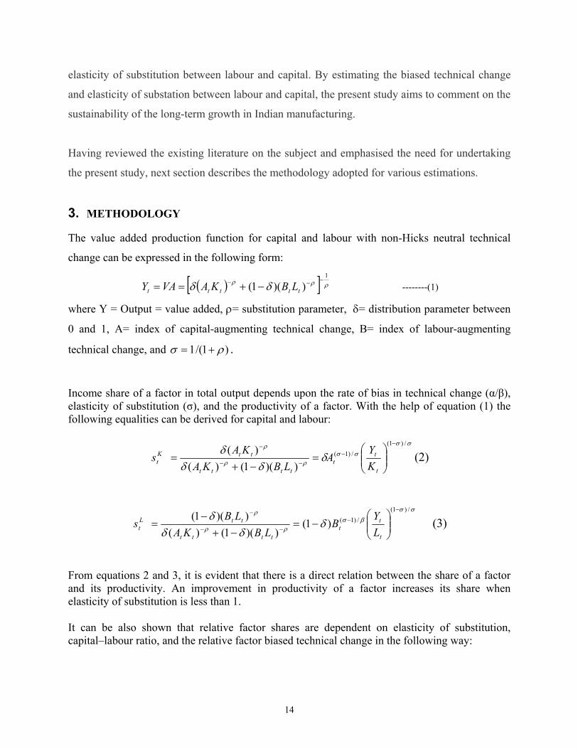
3. METHODOLOGY The value added production function for capital and labour with non-Hicks neutral technical

change can be expressed in the following form:

( )[ ] ρρρ δδ1

))(1(−−− −+== ttttt LBKAVAY --------(1)

where Y = Output = value added, ρ= substitution parameter, δ= distribution parameter between

0 and 1, A= index of capital-augmenting technical change, B= index of labour-augmenting

technical change, and )1/(1 ρσ += .

Income share of a factor in total output depends upon the rate of bias in technical change (α/β), elasticity of substitution (σ), and the productivity of a factor. With the help of equation (1) the following equalities can be derived for capital and labour:

σσσσ

ρρ

ρ

δδδ

δ/)1(

/)1(

))(1()()(

−

−−−

−

=

−+=

t

tt

tttt

ttKt K

YA

LBKAKA

s (2)

σσβσ

ρρ

ρ

δδδ

δ/)1(

/)1()1())(1()(

))(1(−

−−−

−

−=

−+−

=t

tt

tttt

ttLt L

YB

LBKALB

s (3)

From equations 2 and 3, it is evident that there is a direct relation between the share of a factor and its productivity. An improvement in productivity of a factor increases its share when elasticity of substitution is less than 1. It can be also shown that relative factor shares are dependent on elasticity of substitution, capital–labour ratio, and the relative factor biased technical change in the following way:

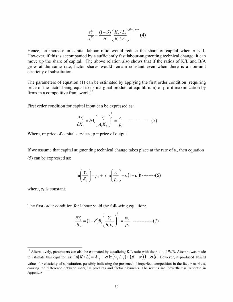
15

σσ

δδ

/)1(

//)1(

−

−=

tt

ttKt

Lt

ABLK

ss (4)

Hence, an increase in capital–labour ratio would reduce the share of capital when σ < 1. However, if this is accompanied by a sufficiently fast labour-augmenting technical change, it can move up the share of capital. The above relation also shows that if the ratios of K/L and B/A grow at the same rate, factor shares would remain constant even when there is a non-unit elasticity of substitution. The parameters of equation (1) can be estimated by applying the first order condition (requiring price of the factor being equal to its marginal product at equilibrium) of profit maximization by firms in a competitive framework.12

First order condition for capital input can be expressed as:

t

t

tt

tt

t

t

pr

KAY

AKY

=

=

∂∂ σ

δ

1

------------ (5)

Where, r= price of capital services, p = price of output.

If we assume that capital augmenting technical change takes place at the rate of α, then equation

(5) can be expressed as:

( )tpr

KY

t

t

t

t σασγ −+

+=

1lnln 1 --------(6)

where, γ1 is constant.

The first order condition for labour yield the following equation:

( )t

t

tt

tt

t

t

pw

LBY

BLY

=

−=

∂∂ σ

δ

1

1 ------------(7)

12 Alternatively, parameters can also be estimated by equalizing K/L ratio with the ratio of W/R. Attempt was made to estimate this equation as: ( ) ( ) ( )( )trwLK tt σαβσλ −−++= 1/ln/ln

3. However, it produced absurd

values for elasticity of substitution, possibly indicating the presence of imperfect competition in the factor markets, causing the difference between marginal products and factor payments. The results are, nevertheless, reported in Appendix.

16

Where, w=wage rate.

Assuming labour augmenting technical change at the rate of β, equation (7) can be expressed

as13:

( )tpw

LY

t

t

t

t σβσγ −+

+=

1lnln 2 -------- (8)

Where γ1 & γ2 are constants.

Attempt is also made to decompose the output growth with the help of the following formula

derived from equation (1):

( ) ( )

−+

∂+

∂

−+

∂

=

∂ ρρρρ

δβαδδδBKY

AKYT

LL

BLY

KK

AKY

YY 11 ---(9)

The factors influencing the intensity of a factor use and its share can be classified into two broad

categories: technological change and factors’ prices. An attempt has been made in this study to

decompose the factor intensity of labour and capital and their income shares into these two

sources.

To estimate the share of capital (SK) and its intensity (K/Y), the following equations have been

used, derived from equation (3):

( ) ( )tprSK σασγ −−

−+−= 1ln1)ln( 1 --------(11)

( )tpr

YK σασγ −−

−−=

1lnln 1 ---------(12)

13 Nothing much can be predicted on the relative size of elasticity of substitution obtained through marginal product of labour and capital equations, though Berndt (1976) pointed out that estimates based on the marginal product of labour equation may yield higher estimates of the elasticity of substitution than estimates based on the marginal product of capital.

17

Alternatively, intensity of capital and its share have also been decomposed through the use of

growth equations as mentioned later.

Similarly, for estimating share of labour (SL) and its intensity (L/Y), the following equations

have been used, which are derived from equation (5):

( ) ( )tpwSL σβσγ −−

−+−= 1ln1)ln( 2 -----------(13)

( )tpw

YL σβσγ −−

−−=

1lnln 2 ---------(14)

4. DATA AND VARIABLES Sources of data

To estimate the parameters of production function for aggregate manufacturing, the data for

period from 1973–74 through 2001–02 has been utilized.14 The entire period has been subdivided

into three period viz. 1973-79, 1980-91 and1992-01, roughly corresponding to pre and post

reforms period. The data has been drawn mainly from the Annual Survey of Industries (ASI). In

addition, data have also been drawn from other sources including Chandhok (1990), various

publications of National Accounts Statistics, and the RBI bulletins.

Construction of variables

Inputs: For estimating parameters of value added production function, total expenses have been

divided into two broad categories: labour (l), and capital (K). The price index of labour has been

derived by dividing the “total emoluments” by the “total persons engaged.” Assuming that the

flow of services is proportional to stock, ‘perpetual inventory method’ has been used to create a

time series on real capital stock [Christensen and Jorgenson 1969]:

1,)1( −−+= tiiitit KdIK ……………(15)

14 Throughout the study, the variables used for analysis pertains to financial year even if it is mentioned in a fashion of calendar year. For instance, 1973-74 may found to be written just as 1973.

18

Where Kit = the real capital stock of category i at year t; Iit = the real value of net investment on

category i at time t; and di = 1/ni, where ni = economic life of asset i, shows a constant rate of

depreciation of asset i over its lifespan.

To apply the ‘perpetual inventory method’, one requires: (i) benchmark capital stock, (ii) annual

investment, (iii) life of capital assets, and (iv) price of capital assets. The benchmark capital

stock (1989–90) has been calculated by applying the ‘all-India’ ratio of fixed capital stock

(constant prices) to the net fixed capital stock (current prices) for 1973–74. To arrive at the

benchmark capital stock (constant prices) for 1973–74, ’gross net ratio’ was calculated from the

RBI bulletin (1976), and the gross fixed capital stock was divided by the average price of capital

assets from 1958 through 1973. The annual gross investment series was constructed by adding

depreciation to the net fixed capital stock. By deflating the annual gross investment series with

the index of capital price, annual real investment for each year was calculated. To deflate the

annual investment series, following Goldar (1986) and Das (2003), a weighted wholesale price

index of construction and machinery was constructed; weights being the proportion of their share

in capital stock during 1973–74. An implicit price deflator for investment in construction was

prepared from the National Account Statistics. Price index of machinery was used as a proxy of

machinery price index. Life of capital stock was assumed to be 25 years, depreciating at the

constant rate of 4 per cent per annum. The price of each capital input was computed to reflect

“user cost of capital.” Because a well-developed rental market for capital does not exist, the price

of capital service ‘i’ – (Pki) – was derived indirectly as:

)( iniki dRPP += …(16)

Where Pni = price of investment goods i, R = current interest rate (long-term lending rate of

IDBI), di = depreciation rate of assets i, (di = 1/ni, where ni = economic life of the asset i).

Output in present study refers to the “value added” for the aggregate manufacturing industry.

The wholesale price index (1981–82 prices) of all commodities has been applied to deflate the

output of the aggregate manufacturing industry.

Stationarity and cointegration of variables

Because the analysis is based on time series data, it was necessary to ensure that the variables

used in the model be cointegrated. For variables to be cointegrated, it was necessary that the

19

variables used in the model be either stationary or integrated of the same order. An attempt was

made to test the stationarity of each variable with the help of ‘augmented Dickey-Fuller’ unit

root test.15 The results show that the time series of all variables are non-stationary because the

ADF Test statistics exceeds the 5% critical value in all the cases (Table 1). But all the time series

were found to be integrated of order one (at first difference), i.e., I (1). Since all the times series

are integrated of the same order, they are expected to be cointegrated as well. To confirm that the

variables of a regression are cointegrated16, we performed the Johansen’s (1995) test.17 The null

hypothesis of no-cointegration was tested with the help of trace statistics. In all the cases, the null

hypotheses of no-cointegration was rejected as the trace statistics turned out to be greater than

5% critical value (Table 2). This implies that there exists a cointegration vector, and hence a

long-term relation between the variables of a given regression.

Table1: Augmented Dickey-Fuller test of stationarity

Variables Level ADF Test Statistics

Level 5% Critical Value

First DifferenceADF Test Statistics

First Difference 5% Critical Value

Ln(Y/L) -2.78 -3.60 -3.68 -3.60 Ln(Y/K) -1.87 -3.60 -5.11 -3.60 Ln(w/p) -2.25 -3.61 -4.63 -3.59 Ln(r/p) -2.26 -2.98 -3.71 -2.98 LN(K/L) -2.53 -3.59 -4.32 -3.59 Ln(w/r) -0.95 -3.58 -6.14 -3.59

Note: (i) The lag-length is based on ‘Schwarz Information Criterion’. (ii) Except in case of Ln (Pk/Py), the regressions are with constant and linear trend. For Ln (Pk/Py), however, the regression is without trend. Table 2: Johansen cointegration test

Variables Eigenvalue

Trace Statistic

5% CV

ρ-value of no Cointegration

Cointegration Rank

ln(Y/L) & ln(w/p) 0.82 56.26 25.87 0.00 1 ln(Y/K) & ln(r/p) 0.78 37.93 25.87 0.00 1

Ln (K/L) & ln(w/r) 0.70 35.84 25.87 0.00 1

15 Please see reference for technical details. 16 The purpose of the cointegration test is to determine whether a group of non-stationary series is cointegrated or not. 17 The regressions are estimated by restricting the linear time trend to lie only in the cointegration space. EViews 5 has been used for estimations.

20

Trends in variables

On the basis of major changes in the economic policy over the years, the present study, besides

analysing the trends over the study period, also analyses and compares the trends across the

following three sub-periods: 1973/74–79/80, 1980/81–91/92, and 1992/93–01/02.

Table 3: Trends in Select Indicators Period 1973–79 1980–91 1992–01 1973–01

Sl 0.44 0.39 0.28 0.37 Y/L 2.00 2.93 5.56 3.61 w/p 1.01 1.32 1.86 1.43 Y/K 1.77 1.47 1.29 1.48 L/Y 0.50 0.36 0.18 0.33 K/Y 0.57 0.68 0.78 0.69 r/p 1.12 1.06 1.10 1.09 K/L 1.13 2.01 4.39 2.62 w/r 0.90 1.24 1.73 1.33

Source: Authors’ own calculations based on ASI data. All the variables exhibit a mark changes in their magnitudes over the study period (see Table 3

and Figure 1). The share of labour (capital) has declined (increased) sharply over the years.

Starting with 0.44 for the first period (1973-79), it has come down to just 0.28 for the last sub-

period (1992-01). Similar sharp change is noticeable for factor intensities. While labour intensity

(L/Y) has declined persistently, capital intensity has moved up. In other words, average

productivity of labour in Indian manufacturing bears an increasing trend in contrast to the falling

trend in capital intensity. This has resulted an increase in the average real wage rate (w/p) and

fall in the cost of capital (r/p). There exists a gap between the average productivity of factors and

their real cost. The productivity of labour (Y/L) exceeds the wage rate (w/p) by more than two

and a half times over the study period. The gap between the two has been widening over the

years, which could be an indication that marginal productivity is increasing faster than the wage

rate. Likewise, productivity of capital exceeds its real price (r/p), but to much lesser extent than

in case of labour and the difference is falling over the years.

To capture and compare the magnitude of change in the variables over years, growth figures of

the select variables are shown in Table 4. All the variables demonstrate mark and distinct

21

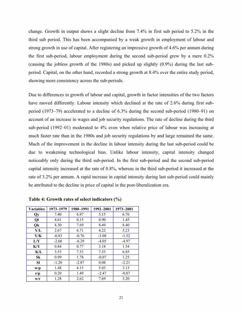
change. Growth in output shows a slight decline from 7.4% in first sub period to 5.2% in the

third sub period. This has been accompanied by a weak growth in employment of labour and

strong growth in use of capital. After registering an impressive growth of 4.6% per annum during

the first sub-period, labour employment during the second sub-period grew by a mere 0.2%

(causing the jobless growth of the 1980s) and picked up slightly (0.9%) during the last sub-

period. Capital, on the other hand, recorded a strong growth at 8.4% over the entire study period,

showing more consistency across the sub-periods.

Due to differences in growth of labour and capital, growth in factor intensities of the two factors

have moved differently. Labour intensity which declined at the rate of 2.6% during first sub-

period (1973–79) accelerated to a decline of 6.3% during the second sub-period (1980–91) on

account of an increase in wages and job security regulations. The rate of decline during the third

sub-period (1992–01) moderated to 4% even when relative price of labour was increasing at

much faster rate than in the 1980s and job security regulations by and large remained the same.

Much of the improvement in the decline in labour intensity during the last sub-period could be

due to weakening technological bias. Unlike labour intensity, capital intensity changed

noticeably only during the third sub-period. In the first sub-period and the second sub-period

capital intensity increased at the rate of 0.8%, whereas in the third sub-period it increased at the

rate of 3.2% per annum. A rapid increase in capital intensity during last sub-period could mainly

be attributed to the decline in price of capital in the post-liberalization era.

Table 4: Growth rates of select indicators (%) Variables 1973–1979 1980–1991 1992–2001 1973–2001

Qy 7.40 6.87 5.15 6.76 Ql 4.61 0.15 0.90 1.45 Qk 8.30 7.69 8.49 8.40

Y/L 2.67 6.71 4.22 5.23 Y/K -0.83 -0.76 -3.08 -1.52 L/Y -2.60 -6.29 -4.05 -4.97 K/Y 0.84 0.77 3.18 1.54

K/L 3.53 7.53 7.53 6.85 Sk 0.99 1.78 -0.07 1.25 Sl -1.20 -2.87 0.08 -2.21 w/p 1.48 4.15 5.03 3.13 r/p 0.20 1.49 -2.47 -0.07 w/r 1.28 2.62 7.69 3.20

22

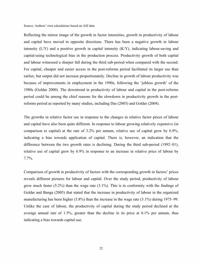
Source: Authors’ own calculations based on ASI data Reflecting the mirror image of the growth in factor intensities, growth in productivity of labour

and capital have moved in opposite directions. There has been a negative growth in labour

intensity (L/Y) and a positive growth in capital intensity (K/Y), indicating labour-saving and

capital-using technological bias in the production process. Productivity growth of both capital

and labour witnessed a sharper fall during the third sub-period when compared with the second.

For capital, cheaper and easier access in the post-reforms period facilitated its larger use than

earlier, but output did not increase proportionately. Decline in growth of labour productivity was

because of improvements in employment in the 1990s, following the ‘jobless growth’ of the

1980s (Goldar 2000). The downtrend in productivity of labour and capital in the post-reforms

period could be among the chief reasons for the slowdown in productivity growth in the post-

reforms period as reported by many studies, including Das (2003) and Goldar (2004).

The growths in relative factor use in response to the changes in relative factor prices of labour

and capital have also been quite different. In response to labour growing relatively expensive (in

comparison to capital) at the rate of 3.2% per annum, relative use of capital grew by 6.9%,

indicating a bias towards application of capital. There is, however, an indication that the

difference between the two growth rates is declining. During the third sub-period (1992–01),

relative use of capital grew by 6.9% in response to an increase in relative price of labour by

7.7%.

Comparison of growth in productivity of factors with the corresponding growth in factors’ prices

reveals different pictures for labour and capital. Over the study period, productivity of labour

grew much faster (5.2%) than the wage rate (3.1%). This is in conformity with the findings of

Goldar and Banga (2005) that stated that the increase in productivity of labour in the organized

manufacturing has been higher (5.8%) than the increase in the wage rate (3.1%) during 1975–99.

Unlike the case of labour, the productivity of capital during the study period declined at the

average annual rate of 1.5%, greater than the decline in its price at 0.1% per annum, thus

indicating a bias towards capital use.

23

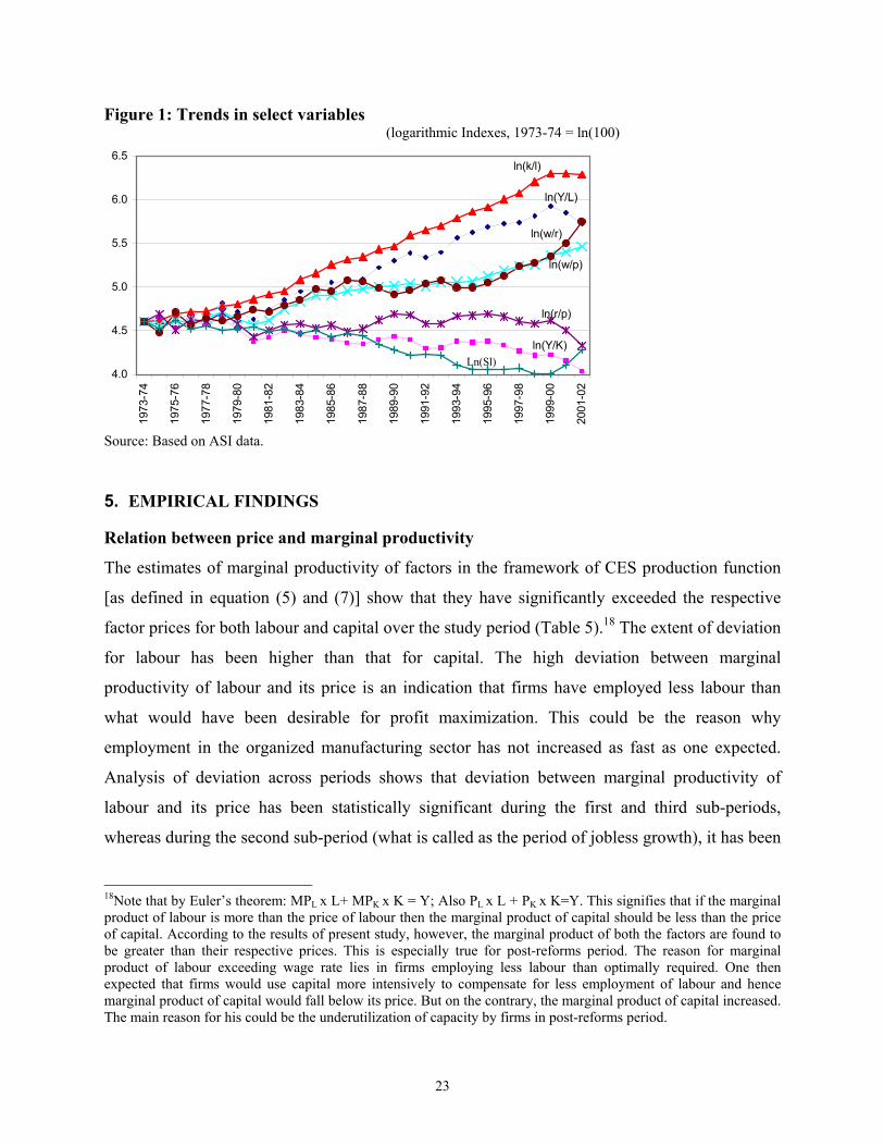
Figure 1: Trends in select variables (logarithmic Indexes, 1973-74 = ln(100)

ln(Y/L)

ln(Y/K)

ln(k/l)

ln(w/p)

ln(r/p)

ln(w/r)

Ln(Sl)4.0

4.5

5.0

5.5

6.0

6.519

73-7

4

1975

-76

1977

-78

1979

-80

1981

-82

1983

-84

1985

-86

1987

-88

1989

-90

1991

-92

1993

-94

1995

-96

1997

-98

1999

-00

2001

-02

Source: Based on ASI data. 5. EMPIRICAL FINDINGS Relation between price and marginal productivity

The estimates of marginal productivity of factors in the framework of CES production function

[as defined in equation (5) and (7)] show that they have significantly exceeded the respective

factor prices for both labour and capital over the study period (Table 5).18 The extent of deviation

for labour has been higher than that for capital. The high deviation between marginal

productivity of labour and its price is an indication that firms have employed less labour than

what would have been desirable for profit maximization. This could be the reason why

employment in the organized manufacturing sector has not increased as fast as one expected.

Analysis of deviation across periods shows that deviation between marginal productivity of

labour and its price has been statistically significant during the first and third sub-periods,

whereas during the second sub-period (what is called as the period of jobless growth), it has been

18Note that by Euler’s theorem: MPL x L+ MPK x K = Y; Also PL x L + PK x K=Y. This signifies that if the marginal product of labour is more than the price of labour then the marginal product of capital should be less than the price of capital. According to the results of present study, however, the marginal product of both the factors are found to be greater than their respective prices. This is especially true for post-reforms period. The reason for marginal product of labour exceeding wage rate lies in firms employing less labour than optimally required. One then expected that firms would use capital more intensively to compensate for less employment of labour and hence marginal product of capital would fall below its price. But on the contrary, the marginal product of capital increased. The main reason for his could be the underutilization of capacity by firms in post-reforms period.

24

statistically non-significant. For capital, the deviation has been statistically significant only

during the third sub-period, indicating that capital in the post-reforms period (till the early 2000s)

has been slightly under-deployed.

Table 5: Marginal productivity and price of factor

Period dY/dL (w/p) (dY/dL) -

(w/p) dY/dK (r/p) (dY/dK)-

(r/p)

1973–79 1.19 1.01 0.18

(4.97) 1.12 1.12 0.0

(0.0)

1980–91 1.33 1.32 0.01

(0.34)* 1.09 1.06 0.02

(1.83)*

1992–01 2.23 1.86 0.37

(2.98) 1.20 1.10 0.10

(7.19)

1973–01 1.61 1.43 0.18

(3.26) 1.13 1.09 0.04

(3.95) Note: (i) Figures in parenthesis indicate t-statistics. (ii) * indicates non-significance of t-statistics at 5% level.

Figures 2 and 3 trace the marginal productivity of factors with their respective prices. For labour,

the gap between marginal productivity and its price has widened significantly after 1989, with

the exception of the last two years. Marginal productivity of labour in the post-reforms period

increased considerably, possibly because of labour working with larger capital. Even though the

price of labour increased too, it was much slower than the rise in productivity. The rising gap

between marginal productivity of labour and the wage rate can be pinned to rigid labour laws,

which prevented firms from employing enough labour to equate its marginal productivity with

price. In other words, in the post-reforms period, firms increasingly refrained from hiring labour,

and sacrificed profit maximization. That labour was being paid less than their marginal products

also indicates that their transfer price (wage) in the unorganized sector would be even smaller.

This perhaps highlights the need for bringing a larger number of unorganized industries within

the ambit of the organized ones to promote labour welfare further.

Though job security regulations have adversely affected employment growth in the 1990s, they

don’t seem to be the main reason for the jobless growth of the 1980s. The small gap between

marginal productivity of labour and its price during the 1980s indicates that job security

regulation had little role to play in jobless growth. If job security regulations had indeed caused

jobless growth, marginal productivity of labour would have been higher than the wage rate

because firms would have employed less labour than what would have been optimally desirable.

25

It would, therefore, be appropriate to conclude that increase in wage rate was mainly because of

jobless growth of the 1980s.

Figure 2: Trends in marginal productivity of labour and its wage rate

0.80

1.10

1.40

1.70

2.00

2.30

2.60

2.90

1973

1975

1977

1979

1981

1983

1985

1987

1989

1991

1993

1995

1997

1999

2001

(w/p) dY/dL

Note: Marginal productivity of labour (dY/dL) is estimated from the first order condition of profit maximization as

mentioned in equation 7.

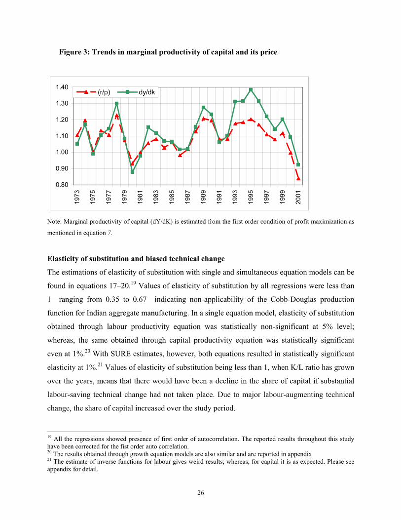
The rise in difference between marginal productivity of capital and its price in the post-reforms

period indicates that either capital has also been employed less optimally or that obsolescence

arising from liberalisation has resulted in a fall in measured productivity as predicted in Virmani

(2005) and Virmani (2006 b). Hence, there is a scope for increasing the employment of capital in

manufacturing. It will be interesting to note that marginal productivity of capital and its price

have been moving in sync with each other. Employment of capital has, thus, been sensitive to

change in its price. It is only for a brief period, around the mid 1990s, that the difference between

marginal productivity of capital its price grew relatively large.

26

Figure 3: Trends in marginal productivity of capital and its price

0.80

0.90

1.00

1.10

1.20

1.30

1.4019

73

1975

1977

1979

1981

1983

1985

1987

1989

1991

1993

1995

1997

1999

2001

(r/p) dy/dk

Note: Marginal productivity of capital (dY/dK) is estimated from the first order condition of profit maximization as

mentioned in equation 7.

Elasticity of substitution and biased technical change

The estimations of elasticity of substitution with single and simultaneous equation models can be

found in equations 17–20.19 Values of elasticity of substitution by all regressions were less than

1—ranging from 0.35 to 0.67—indicating non-applicability of the Cobb-Douglas production

function for Indian aggregate manufacturing. In a single equation model, elasticity of substitution

obtained through labour productivity equation was statistically non-significant at 5% level;

whereas, the same obtained through capital productivity equation was statistically significant

even at 1%.20 With SURE estimates, however, both equations resulted in statistically significant

elasticity at 1%.21 Values of elasticity of substitution being less than 1, when K/L ratio has grown

over the years, means that there would have been a decline in the share of capital if substantial

labour-saving technical change had not taken place. Due to major labour-augmenting technical

change, the share of capital increased over the study period.

19 All the regressions showed presence of first order of autocorrelation. The reported results throughout this study have been corrected for the fist order auto correlation. 20 The results obtained through growth equation models are also similar and are reported in appendix 21 The estimate of inverse functions for labour gives weird results; whereas, for capital it is as expected. Please see appendix for detail.

27

Single Equation Estimates

)9.2()1.1()3.3(038.0)/(35.04737.0)/( TpwLnLYLn ++=

− …(17)

059.0;42.0)(;58.0)(;86.1;35.0;97.0;46.1 2 ======= βδδρσ LKRDw

)0.23()6.14()3.44(0145.0)/(673.0553.0)/(−

−+= TprLnKYLn …(18)

044.0;56.0)(;44.0)(;486.0;67.0;98.0;86.1 2 −======= αδδρσ LKRDw

SURE Estimates

)6.13()6.14()9.3(028.0)/(635.0550.0)/( TpwLnLYLn ++= …(19)

712.1;075.0;42.0;58.0;575.0;64.0;97.0;45.1 0

2 ===−=−==== ALKRDw βδδρσ

)4.23()6.14()3.45(015.0)/(635.0556.0)/(−

−+= TprLnKYLn …(20)

712.1;041.0;42.0;58.0;575.0;64.0;98.0;84.1 02 =−==−=−==== ALKRDw αδδρσ

Findings indicate a strong bias in technical change (α/β) with varying degrees across equations.

Labour saving was found to have occurred in the rage of 5.9% to 7.5%; whereas, capital use

increased between 4.1% and 4.4%.22 On an average, labour saving occurred at the annual rate of

6.7%; whereas, capital use increased by 4.3% per annum. Strong labour-augmenting technical

change caused share of capital to increase fast. If the value of elasticity of substitution between

labour and capital had not been less than 1, the increase in share of capital would have been even

sharper with the rise in K/L ratio.

Not only that the elasticity of substitution in the Indian manufacturing sector is found to be less

than 1, but it has also come down over the years. Dividing the study period in pre- and post-

reforms years, one find that elasticity of substitution has come down in the later period. In single

equation estimate for capital, one finds that the value of elasticity of substitution declined from

22 Growth equations also report similar ranges, as can be seen in Appendix

28

an average of 0.68 during 1973–90 to an average of 0.66 during 1991–2001. SURE estimates

showed even larger decline (from 0.62 to 0.56) between pre- and post-reforms period. The labour

equation gave negative elasticity for post-reform period, which can be ignored as this was

statistically not significant at 5% level. Decline in value of elasticity of substitution in the post-

reforms period, when K/L ratio grew up considerably, was enough to outweigh the effect of any

labour-augmenting technical change that resulted in negative growth in the share of capital

during the 1992 –2001 period.

Like the elasticity of substitution, the technical bias is also found to have declined in post-

reforms as compared to pre-reforms period. Dividing the study period in this fashion revels that

bias in labour-saving has declined from 11% during 1973 –1990 to 4.2% during 1991–2001

period in case of single equation model. SURE model also reported a decline in labour savings

from 7.7% to 6.8% between pre- and post-reforms period. Relatively higher growth in labour

employment during post-reforms period thus may be attributed to the decline in labour-saving

technical bias. Similarly, the capital using technical bias too declined (in absolute terms) from -

4.8% to -4.4% in the single equation model and from -4.0% to -3.2% in the SURE model

between pre- and post-reforms period. Declining degree of bias in technical change coupled with

falling elasticity of substitution indicates that increase (decrease) in share of capital (labour) will

be contained in the future even if K/L ratio goes on increasing.

Period-wise change in elasticity of substitution and technical change

Single Equation Estimates

)20011991()86.2()901973()5.2()20011991()901973()7.1()5.1(

069.0045.0)/(642.0)/(594.0347.0)/(−−

−−−

++−+= TTpwLnpwLnLYLn (21)

.042.0;110.0;64.0;59.0;97.0;84.1 2121

2 ==−==== ββσσRDw

)20011991()9.20()901973()7.11()20011991()9.9()901973()5.10()6.35(015.0015.0)/(657.0)/(685.0554.0)/(

−−−−−−

−−++= TTprLnprLnKYLn (22)

044.0;048.0;66.0;69.0;98.0;90.1 2121

2 −=−===== αασσRDw

29

SURE Estimates

)20011991()6.4()901973()5.3()20011991(1.8)901973()4.9()2.4(030.0029.0)/(559.0)/(624.0532.0)/(

−−−−

++++= TTpwLnpwLnLYLn (23)

.068.0;077.0;56.0;62.0;97.0;44.1 2121

2 ====== ββσσRDw

)20011991()0.18()901973()3.10()20011991()1.8()901973()4.9()3.31(014.0015.0)/(559.0)/(624.0561.0)/(

−−−−−−

−−++= TTprLnprLnKYLn (24)

.032.0;040.0;56.0;62.0;98.0;80.1 21212 −=−===== αασσRDw

Determinants of labour intensity and its share

Labour intensity has declined at 5% per annum during 1973–2001.23 Decomposition analysis,

presented in Table 6, shows that 64% of this decline is attributable to technical change and the

remaining 36% to increase in wage rate. Significantly, the share of wage in declining job

intensity is steeply increasing over the years. In the first sub-period (1973–1979), when labour

intensity declined at 2.6% per annum, the contribution of wage amounted to only 25%. In the

second sub-period (1980–1991), when labour intensity witnessed a sharper decline at the rate of

6.3% per annum, the contribution of wage moved up to 48.5%. In the last sub-period (1992-

2001), even with the moderation in the decline in labour intensity to 4% per annum, the

contribution of wage surged to 53.3%. So now both increase in wage rate and wakening

technological factors are almost equally contributing to the decline in labour intensity /

employment.

During 1973-01, the share of labour in value-added declined at the rate of 2.2% per annum

(lower than labour intensity at -5.0%). Decomposition analysis indicates that the two main

determinants namely, technical change and wage rate, played opposite roles in this decline.

While technical change lowered the labour share by 165.1%; rising labour costs made it move in

opposite direction by 65.1%, due to inelastic demand for labour. In the first two sub-periods, the

share of labour fell despite the rising price of labour because the effect of technical change was

more powerful the effect of the price of labour. In the last sub-period, however, the rising price

23 Assuming constant rerun to scale, labour and capital intensities are taken to represent their employment in the production process.

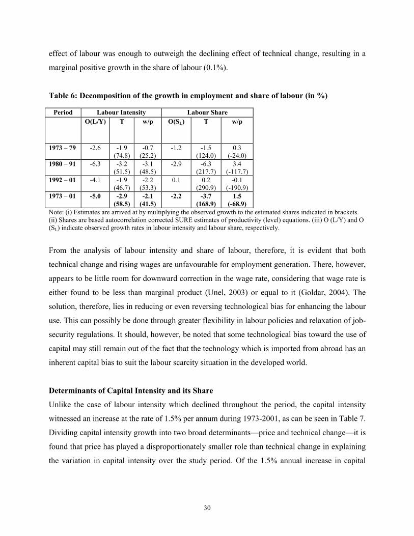
30

effect of labour was enough to outweigh the declining effect of technical change, resulting in a

marginal positive growth in the share of labour (0.1%).

Table 6: Decomposition of the growth in employment and share of labour (in %)

Period Labour Intensity Labour Share O(L/Y) T w/p O(SL) T w/p

1973 – 79 -2.6 -1.9 (74.8)

-0.7 (25.2)

-1.2 -1.5 (124.0)

0.3 (-24.0)

1980 – 91 -6.3 -3.2 (51.5)

-3.1 (48.5)

-2.9 -6.3 (217.7)

3.4 (-117.7)

1992 – 01 -4.1 -1.9 (46.7)

-2.2 (53.3)

0.1 0.2 (290.9)

-0.1 (-190.9)

1973 – 01 -5.0 -2.9 (58.5)

-2.1 (41.5)

-2.2 -3.7 (168.9)

1.5 (-68.9)

Note: (i) Estimates are arrived at by multiplying the observed growth to the estimated shares indicated in brackets. (ii) Shares are based autocorrelation corrected SURE estimates of productivity (level) equations. (iii) O (L/Y) and O (SL) indicate observed growth rates in labour intensity and labour share, respectively.

From the analysis of labour intensity and share of labour, therefore, it is evident that both

technical change and rising wages are unfavourable for employment generation. There, however,

appears to be little room for downward correction in the wage rate, considering that wage rate is

either found to be less than marginal product (Unel, 2003) or equal to it (Goldar, 2004). The

solution, therefore, lies in reducing or even reversing technological bias for enhancing the labour

use. This can possibly be done through greater flexibility in labour policies and relaxation of job-

security regulations. It should, however, be noted that some technological bias toward the use of

capital may still remain out of the fact that the technology which is imported from abroad has an

inherent capital bias to suit the labour scarcity situation in the developed world.

Determinants of Capital Intensity and its Share

Unlike the case of labour intensity which declined throughout the period, the capital intensity

witnessed an increase at the rate of 1.5% per annum during 1973-2001, as can be seen in Table 7.

Dividing capital intensity growth into two broad determinants—price and technical change—it is

found that price has played a disproportionately smaller role than technical change in explaining

the variation in capital intensity over the study period. Of the 1.5% annual increase in capital

31

intensity, as much as 97.4% of the change came from technical change alone, limiting the

contribution of price factor to only 2.6%.

Sub-period wise analysis shows wide variations in the contributions of the two determinants,

resulting majorly due to varying contributions of price factor. In the first sub-period (1973-79),

when capital intensity increased by 0.8%, the price factor contributed negatively to the capital

intensity to a extent of 9%. In the second sub-period (1980-1991) when capital intensity again

declined by 0.8% per annum, the contribution of price factor had slumped to minus 171%. If it

was not for the sharp increase in contribution of technology (271%) (Possibly on account of

strengthening of labour laws and thereby creating a bias towards capital use) during this period,

the intensity of capital would have suffered adversely. In the third sub-period (1992-2001),

contribution of price factor not only became positive for the first time but it also turned

significant at 51%, resulting in sharper growth in intensity of capital to the extent of 3.2% per

annum. Continuing downward pressure on price of capital along with the stringent labour laws,

hence, may further increase the intensity of capital in future.

Table 7: Decomposition of the growth in deployment and share of capital Period K-Intensity K-Share

O(K/Y) T r/p O(SK) T r/p 1973-79 0.8 0.9

(109.3) -0.1

(-9.3) 1.0 0.9

(95.3) 0.1

(4.7) 1980-91 0.8 2.1

(271.8) -1.3

(-171.8) 1.8 1.3

(73.4) 0.5

(26.6) 1992-01 3.2 1.6

(48.9) 1.6

(51.1) -0.1 -0.2

(250.3) 0.1 (-

150.3) 1973-01 1.5 1.5

(97.2) 0.0

(2.8) 1.3 1.3

(101.7) -0.0

(-1.7) Note: (i) Estimates are arrived by multiplying the observed growth to the estimated shares indicated in brackets. (ii) Shares are based on autocorrelation corrected SURE estimates of productivity (level) equations. (iii) O (K/Y) and O (SK) indicate observed growth rates in labour intensity and labour share, respectively.

Along with the increase in its intensity, capital also witnessed an increase in its share in the

value-added by 1.3% per annum during the study period. Virtually, the entire increase is

attributable to technical change, as wide fluctuations in share of price factor across sub-periods

nullified the price effects. In first and second sub-periods, the increase in price of capital had

contributed to increase in share of capital by 5% and 27%, respectively. However, in the third

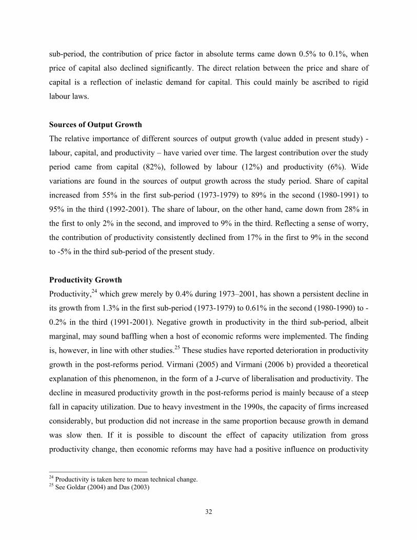
32

sub-period, the contribution of price factor in absolute terms came down 0.5% to 0.1%, when

price of capital also declined significantly. The direct relation between the price and share of

capital is a reflection of inelastic demand for capital. This could mainly be ascribed to rigid

labour laws.

Sources of Output Growth

The relative importance of different sources of output growth (value added in present study) -

labour, capital, and productivity – have varied over time. The largest contribution over the study

period came from capital (82%), followed by labour (12%) and productivity (6%). Wide

variations are found in the sources of output growth across the study period. Share of capital

increased from 55% in the first sub-period (1973-1979) to 89% in the second (1980-1991) to

95% in the third (1992-2001). The share of labour, on the other hand, came down from 28% in

the first to only 2% in the second, and improved to 9% in the third. Reflecting a sense of worry,

the contribution of productivity consistently declined from 17% in the first to 9% in the second

to -5% in the third sub-period of the present study.

Productivity Growth

Productivity,24 which grew merely by 0.4% during 1973–2001, has shown a persistent decline in

its growth from 1.3% in the first sub-period (1973-1979) to 0.61% in the second (1980-1990) to -

0.2% in the third (1991-2001). Negative growth in productivity in the third sub-period, albeit

marginal, may sound baffling when a host of economic reforms were implemented. The finding

is, however, in line with other studies.25 These studies have reported deterioration in productivity

growth in the post-reforms period. Virmani (2005) and Virmani (2006 b) provided a theoretical

explanation of this phenomenon, in the form of a J-curve of liberalisation and productivity. The

decline in measured productivity growth in the post-reforms period is mainly because of a steep

fall in capacity utilization. Due to heavy investment in the 1990s, the capacity of firms increased

considerably, but production did not increase in the same proportion because growth in demand

was slow then. If it is possible to discount the effect of capacity utilization from gross

productivity change, then economic reforms may have had a positive influence on productivity

24 Productivity is taken here to mean technical change. 25 See Goldar (2004) and Das (2003)

33

growth. Our inability to separate out the effects of capacity utilization from gross productivity

change is the main limitation of present study and could be a topic of research in the future. But

it may be safe to argue that reforms have affected productivity growth favourably, and hence,

these reforms should be continued to increase the cost competitiveness of the manufacturing

sector while ensuring sustainability of its output growth.

Table 8: Contributory factors to the output growth (in %)

Note: Growth rates are calculated by multiplying the observed values of the growth in output with the estimated shares. Shares were estimated with the help of coefficients derived from SURE models.

Sustainability of Output Growth

Much of the growth in output of the manufacturing sector in the post-reforms period till the

beginning of 2000s has come on the back of spiralling growth in the capital–labour ratio. The

availability of relatively cheaper capital in the post-reforms period provided firms with an

opportunity to move toward capital-intensive technology and curtail the use of labour. Larger use

of capital not only raised its share in output growth but also increased the productivity of labour,

thereby helping growth in output. Thus, how long can firms accelerate output growth by

increasing capital–labour ratio? The answer depends upon the value of elasticity of substitutions

on the one hand and biased technical change on the other. Since technical change is found to be

strongly labour-saving, it may be argued that growth in capital–labour ratio is sustainable even if

the value of elasticity of substitution is less than 1. With increase in capital–labour ratio, when

elasticity of substitution is less than 1 and technical change is considerably labour- saving,

marginal productivity of capital may not decline to zero. This is because a strong labour savings

technical change would offset the fall in marginal productivity of capital on account of large

Period Growth in Y (actual)

Share in growth (AR1)

Capital Labour Tech 1973 – 79 7.40 4.09

(55) 2.06 (28)

1.25 (17)

1980 – 90 6.87 6.11 (89)

0.15 (2)

0.61 (9)

1991 – 01 5.15 4.91 (95)

0.48 (9)

-0.24 (-5)

1973 – 2001 6.76 5.53 (82)

0.81 (12)

0.42 (6)

34

capital use in presence of less than one value of elasticity of substitution. As long as technical

change is powerful enough to offset the effect of less than 1 value of elasticity of substitution,

growth in capital-labour ratio and output is sustainable.

The present study has, however, found that both elasticity of substitution and the degree of

biased technical change were declining during the 1990s, which is a warning signal for

sustainability of both rising capital–labour ratio and output. The opportunity with firms to

accelerate output growth by increasing capital–labour ratio is thus ceasing because it may not be

too long before marginal productivity of capital comes down to zero. Firms would then be forced

to augment the employment of labour as well as capital for increasing the level of output.

Suppressing the demand for labour would not be possible for too long now. But there is a caveat

to this. If firms continue to be discouraged to employ more labour owing to rigid labour laws,

they may sacrifice the growth in output as they have sacrificed profit maximizing position with

regard to employment of labour for a long time. This, in turn, would put a check on the growth of

output. In other words, the key to unshackling the growth in output as well as employment lies in

doing away with the rigidities in the labour laws.

6. SUMMARY AND CONCLUSION The manufacturing sector is thought to hold a place of unique importance mainly for two

reasons: It can provide large scale employment to labour force increasingly being displaced from

shrinking agriculture sector, and secondly it can help in accelerating the GDP growth by virtue of

its forward and backward linkages with other sectors of the economy. The present study attempts

to identify the factors which can help in unlocking the employment potential of the

manufacturing sector. An attempt is then made to identify the various sources of output growth.

Since productivity is one of the most important factors, attempt is made to examine if economic

reforms unleashed from 1991 had any impact on it. And lastly, study attempts to analyse the

growth in output in manufacturing sector is sustainable in the face of ever increasing capital

labour ratio. Analyses are based on CES production function, utilising the ASI data for a period

from 1973/74 to 2001/02. To examine the impact of various economic policy over the years, the

present study also analyses variables across the following three sub-periods: 1973/74–79/80 (first

sub-period), 1980/81–91/92 (second sub-period), and 1992/93–01/02 (third sub-period).

35

Justification for applying CES production function is provided by the findings of the value of

elasticity of substitution and technical change. Neither the elasticity of substitution between

labour and capital was found to be 1 nor was the technical change ‘Hicks neutral,’ thus ruling out

the applicability of Cobb-Douglas production function for Indian manufacturing. The value of

elasticity of substitution was found to be less much than 1, ranging between 0.35 and 0.67,

depending upon the method of estimation. Similarly, technical change was biased with labour

saving occurring at 6.7% and capital use increasing at 4.3 per cent per annum. Further, both

elasticity of substitution and degree of biased technical change have declined in the post-reforms

period, indicating that decline in share of labour could be arrested in future.

Determinants of factor employment and their share have been identified in terms of technical

change and factor prices. Decomposition of change in labour employment (L/Y), which declined

at 5% per annum in 1973–01, reveals that 64% of the decline was due to labour-saving technical

change and the remaining was due to rise in real wage rate. Wage rate, however, is increasingly

becoming an important variable that determines employment. In fact, its share has moved from

25% in 1973–79 to 53.3% in 1992–01. Thus, now both biased technical change and rising wages

have become equally important determinants of manufacturing employment. Increasing the

employment by reduction of wage rate however may not be possible as the wage rate is found to

be smaller than the marginal product of labour. The solution, therefore, lies in reducing the

degree of technical bias by making labour laws more flexible and loosening the job security

regulations. Income share of labour, witnessing a fall at 2.2% per annum during the study period,

has been the net result of biased technology (taking the share up) and wage rate (taking the share

down). In the first two sub-periods, despite a rising wage rate, the share of labour fell because of

considerable labour-saving technical change. In the last sub-period, however, the price effect was

powerful enough to outweigh the negative effects of technical change, resulting in a marginal

growth in share of labour (0.1%). With the influence of technical bias continuing to weaken and

that of wage rate on the rise, the share of labour may accelerate upwards in future.

Decomposition of the change in capital employment (K/Y), which increased at 1.5% per annum

over the study period, reveals that as much as 97.2% of the increase has been contributed by

36

technical change alone, limiting the contribution of price factor to only 2.8%. As expected, the

price factor strengthened in the post-reforms period, which saw real price of capital falling at 3%

per annum and contributing almost half of the total increase in capital intensity. If capital price

continues to decline further, it may further boost capital intensity and mitigate the effect of a

declining technical bias in its favour. Income share of capital has been primarily governed by

technology rather than the price factor over the study period. But the share contribution of price

factor has increased fast over the years. In absolute terms, however, contribution of capital

increased during first and second period and declined during the third sub period. Contribution of

capital moved directly with the price of capital indicating inelastic demand for capital. If the

demand for capital was elastic—as would have happened if the labour policy was flexible—the

growth in share of capital would have been positive even in the post- reforms period.

With view to investigate the issue of employment of factors further, attempt is made to see

whether factors have been paid according to marginal products. Interestingly, it was found that

both labour and capital have been paid lower than their marginal product. The difference was

sharper for labour, indicating that firms stopped employing labour before reaching the profit

maximising situation. Thus, the deviation between marginal productivity of labour and its price

could be the reason for the slow employment in the organised manufacturing sector. If this is the

state of affairs of this sector then it also indicates that wages paid to labourers in the unorganised

sector would be even lower than its marginal productivity. Hence, if the labour welfare

promotion is important objective of the development process, then it becomes necessary to

remove impediments for larger number of manufacturing industries to increase in size and

remove the incentive for large employment intensive organised industries to fragment into

smaller units.

Across-the-sub-period, the analysis shows that deviation of marginal productivity of labour

(MPL) from wages was statistically significant during the first and third periods. During the

second sub-period (what is termed as jobless growth period), the gap between marginal

productivity and wage rate was insignificant, implying that employment was close to optimum.

Job security regulations apparently had minimum influence on jobless growth of the 1980s;

rather, it was due to sharp rise in wages. For if job security regulations caused jobless growth,

37

marginal productivity of labour would have been higher than the wage rate. Even if job security

regulations had not become stringent during the 1980s, firms would have never paid labour more

than their marginal product when wages were rapidly moving upward. For capital, the deviation

between marginal product and its price was statistically significant only during the third sub-

period, which would mean that capital in post-reforms had been underemployed slightly. There

were indications that this correction might be taking place already as investments in recent years

(post the time-period of this study) have risen sharply. It is interesting to observe that the

marginal productivity of capital and its prices moved in close sync with each other.

As far as the sources of output growth was concerned, it was found that much of the growth in

output had come from capital (82%), followed by labour (12%), and productivity (6%). The

share of labour, despite having improved from the 1980s, continued to be low at 9% during

1992–01. In a labour surplus country like India, this is not a welcome sign. Most importantly, the

contribution of productivity had shown a consistent decline from 17% in the first period to 9% in

the second, and to -5% in the third. The negative contribution of productivity can be attributed

mainly to the heavy decline in capacity utilization in the post-reforms period because of the

presence of a time lag between investment and output growth. However, pure productivity,

devoid of the effects of capacity utilization, must have improved in post-reforms. This is

consistent with and supports the “J curve of liberalisation and Productivity” hypothesis proposed

by Virmani (2005).

The findings on sustainability of output growth with rising capital–labour ratio indicate that the

growth in capital–labour ratio itself may not be sustainable in the long run if both elasticity of

substitution and degree of biased technical change continued to decline, as they have been during

the 1990s. With the continuing decline in these two values, marginal productivity of capital

would tend to zero, thus limiting the growth in capital–labour ratio and output. Output growth

then would not sustainable with suppression of labour demand. But if stringent labour laws did

force firms to do so, firms may continue to suppress demand for labour and sacrifice the growth

in output. The J curve of liberalisation and productivity and the growth of manufacturing since

2003-04 suggests that semi-skilled labour intensive growth is still possible. Labour reforms are

38

however essential if we want labour intensive growth on scale large enough to draw labour out of

the low productivity agriculture sector.

REFERENCES Ahluwalia, I.J. (1991), Productivity and Growth in Indian Manufacturing, Delhi: Oxford University Press. Arrow, Kenneth J., Hollis B. Chenery, Bagicha Minhas, and Robert M. Solow (1961), “Capital-Labor Substitution and Economic Efficiency”, Review of Economics and Statistics, Vol. 43 (3), pp. 225-254. Antras Pol (2004) “Is the U.S. Aggregate Production Function Cobb-Douglas? New Estimates of the Elasticity of Substitution”, Contributions to Macroeconomics, The Berkeley Electronic Press. Berndt, Ernst (1976), “Reconciling Alternative Estimates of the Elasticity of Substitution”, Review of Economics and Statistics, 58:1, pp. 59-68. Bosworth, Barry and Susan M. Collins (2007), “Accounting for Growth: Comparing China and India”, Working Paper Number 12943, National Bureau of Economic Research, Cambridge. Bhalotra, Sonia R (1998): “The Puzzle of Jobless Growth in Indian Manufacturing”, Oxford Bulletin of Economics and Statistics, Vol. 60, No. 1. Chandhok, H. L. and the Policy Group (1990), India Database: The Economy, Living Media India, New Delhi. Gujarati, Damodar N. (1995), Basic Econometrics, Third Edition. New York: McGraw-Hill, Inc. Laurits R. Christensen, Dale W. Jorgenson, and Lawrence J. Lau. (1973), “Transcendental Logarithmic Production Frontiers”, Review of Economics and Statistics 55, no. 1 (February): 28-45. Das, D. K. (2003), “Manufacturing Productivity under Varying Trade Regimes: India in the 1980s and 1990s”, Working Paper No. 107, ICRIER, New Delhi, July. Fallon, Peter R., and Robert E.B. Lucas (1991), "The Impact of Changes in Job Security Regulations in India and Zimbabwe", World Bank Economic Review, vol. 5(3). Ghose, Ajit K (1994), “Employment in Organised Manufacturing In India”, Indian Journal of Labour Economics, Vol 37, No 2, pp 143-60. Goldar, B. N. (1986), Productivity Growth in Indian Industry, Allied Publishers, New Delhi. Goldar, B. N. (2000), “Employment Growth in Organized Manufacturing in India”, Economic and Political Weekly, April 1, pp 1191-95. Goldar, B. N. (2000a), “TFP Growth in the Indian Manufacturing in the 1980s”, Economic and Political Weekly, 37(49): 4966-68. Goldar, B. N. and Anita Kumari (2003), “Import Liberalization and Productivity Growth in Indian Manufacturing Industries in the 1990s”, Developing Economies, December, 41(4): 436-60. Goldar B. N. (2004), “Productivity Trends in Indian Manufacturing in the Pre- and Post- Reform periods”, Working Paper No. 137, ICRIER, New Delhi, June. Goldar, B. and R. Banga (2005), “Wage Productivity Relationship in Organised Manufacturing in India: A State-wise Analysis”, The Indian Journal of Labour Economics, Vol. 48, No. 2.

39

Government of India (a), Annual Survey of Industries: Summary Results for Factory Sector, Central Statistical Organization, New Delhi. Government of India (c), National Account Statistics (various issues), Central Statistical Organization, New Delhi. Hsieh, Chang-Tai (2000), “Measuring Biased Technological Change,” Princeton University, mimeo. Jalava, J., Matti Pohjola, Antti Ripatti and Jouko Vilmunen (2005), “Biased Technical Change and Capital-Labour Substitution in Finland, 1902-2003” Discussion Paper No 56, Helsinki Center of Economic Research, University of Helsinki, Helsinki. Johansen, S. (1995), Likelihood-Based Inference in Cointegrated Vector Autoregressive Models, Oxford University Press, Oxford. Lucas, Robert E. (1969), : “Labour-Capital Substitution in U.S. Manufacturing” in The Taxation of Income from Capital, edited by Arnold Harberger and Martin J. Bailey, Washington, DC: The Brookings Institution, pp. 223-274. Maddala, G. S. (1965), “Differential Industry Effects and Differential Factor Effects of Technological Change”, Memo 36, Research Centre in Economic Growth, Stanford University. Nagaraj, R (1994), “Employment and Wages in Manufacturing Industries: Trends, Hypothesis and Evidence”, Economic and Political Weekly, January 22, pp 177-86. Papola, T S (1994), ‘Structural Adjustment, Labour Market, Flexibility and Employment’, Indian Journal of Labour Economics, Vol 37, No 1, pp 3-16. Pradhan G. and K. Barik (1999), “Total Factor Productivity Growth in Developing Economies: A Study of Selected Industries in India”, Economic and Political Weekly, Mumbai, July 31. Reserve Bank of India (1976): RBI Bulletin. Roy, Sudipta Dutta (1998), “Lags in Employment Adjustment and Inter-Industry Differentials: An Analysis Using Dynamic Inter-related Factor Demand Functions”, Discussion Paper No 149, Indira Gandhi Institute of Development Research, Bombay. Solow, R. (1962), “Technical Progress, Capital Formation and Growth”, American Economic Review, 52, 76-86. Tata Services Limited (2003): “Reforms and Productivity Trends in Indian Manufacturing Sector”, Department of Economics and Statistics, Tata Services limited, Mumbai. Trivedi, P., A. Prakash, and D. Sinate (2000), “Productivity in Major Manufacturing Industries in India: 1973-74 to 1997-98,” Development Research Group Study no. 20, Department of Economic Analysis and Policy, Reserve Bank of India, Mumbai. Unel, Bulent (2003), “Productivity Trends in India’s Manufacturing Sectors in the last Two Decades”, IMF Working Paper no. WP/03/22. Virmani, Arvind (2004), Accelerating Growth and Poverty Reduction: A Policy Framework for India's Development. New Delhi, Academic Foundation. Virmani, Arvind (2005) Policy Regimes, Growth and Poverty in India: Lessons of Government Failure and Entrepreneurial Success!, Working Paper No. 170, ICRIER, October 2005. Virmani, Arvind (2006a), “Sustaining Employment and Equitable Growth: Policies For Structural Transformation Of The Indian Economy,” Working Paper No. 3/2006-PC, Planning Commission, March 2006. http://planningcommission.nic.in/reports/wrkpapers/rpwpf.htm.

40

Virmani, Arvind (2006b), “The Dynamics of Competition: Phasing of Domestic and External Liberalisation in India,” Working Paper No. 4/2006-PC, Planning Commission, April 2006.

http://planningcommission.nic.in/reports/wrkpapers/rpwpf.htm.

World Bank (1989), "India: Poverty, Employment and Social Services”, A World Bank Study, Washington D C: The World Bank. World Development Indicators (2007) APPENDIX • Granger causality test for labour shows that the price of labour is not unrelated to its productivity; i.e. it does

affect its productivity. Productivity on the other hand seems to have a relatively marginal effects on wage rate, but this result is not statistically significant at 10% levels. This test for capital, however, shows that the price of capital has little to do with the productivity of capital. However, its productivity seems to play a larger role in determining the price of capital. Thus, it can be argued that capital productivity equation should be relied on more, as far as the value of elasticity of substitution is concerned.

Table A1: Pairwise Granger causality tests (1973-2001) Lag: 1

Null Hypothesis F-Statistic Probability Ln(w/p) does not Granger Cause Ln(Y/L) 0.03 0.86 Ln(Y/L) does not Granger Cause Ln(w/p) 1.18 0.29 T does not Granger Cause Ln(Y/L) 4.14 0.05 LN(Y/L) does not Granger Cause T -23.3 1.00 T does not Granger Cause Ln(w/p) 5.67 0.03 Ln(w/p) does not Granger Cause T -16.79 1.00 Ln(r/p) does not Granger Cause Ln(Y/K) 4.82 0.04 Ln(Y/K) does not Granger Cause Ln(r/p) 0.43 0.52 T does not Granger Cause Ln(Y/K) 6.74 0.02 Ln(Y/K) does not Granger Cause T -23.26 1.00 T does not Granger Cause Ln(r/p) 0.48 0.50 Ln(r/p) does not Granger Cause T -1.46 1.00

Table A2: Production structure of aggregate manufacturing (1973-2001): Single equation estimates

Dept Var Const

Substitution Indicator (Direct or Indirect) T D+

w R2 σ δ(k) δ(l) α/β ρ

a0 Varabl a1 a2 (1-a1)/a1 Ao

delta Bo

(1-delt) (1/σ -1) DLn(Y/L)

0.0250 (1.5) dln(w/p)

0.4827 (1.7)* 1.63 0.07 0.483 0.048 1.072

DLn(Y/K)

-0.0134 (-

3.1)*** dln(r/p) 0.689

(13.5)*** - 2.47 0.87 0.689 -

0.043 0.451 Note (i) Figures in bracket indicate t-statistics. (ii) *** = significant at 1 per cent level; **=significant at 5 per cent level; *= significant at 10 per cent level. (iii)+ refers to autocorrelation corrected DW. Table A3: SURE Estimates of growth equations of productivity (1973-2001)

41

Dept Var Const AR(1) D+

w R -sq σ ρ α/β Varabl Coef(t)

Dln(Y/L)

0.014 (0.9) Dln(w/p)

0.740 (15.3)***

0.06889 (0.3) 1.59 0.03 0.74 0.351 0.052

Dln(Y/K)

-0.013 (-4.2)*** Dln(r/p)

0.740 (15.3)***

-0.3366 (-1.8)* 1.86 0.87 0.74 0.351 -0.050

Note:*** = significant at 1 per cent level; **=significant at 5 per cent level; *= significant at 10 per cent level. + refers to autocorrelation corrected DW. Table A4: Decomposition of the growth in employment and share of labour through growth equations (in %)

Period Labour Intensity Labour Share O(L/Y) T w/p O(SL) T w/p

1973-79 -2.6 -1.5 (56.0)

-1.1 (44.0)

-1.2 -1.7 (138.0)

0.5 (-38.0)

1980-91 -6.3 -2.0 (31.3)

-4.3 (68.7)

-2.9 -12.5 (435.5)

9.6 (-335.5)

1992-01 -4.0 -1.1 (27.3)

-2.9 (72.7)

0.1 1.3 (1535.8)

-1.2 (-1435.8)

1973-01 -5.0 -1.9 (37.7)

-3.1 (62.3)

-2.2 -5.3 (238.9)

3.1 (-138.9)

Note: Estimates are arrived by multiplying the observed growth to the estimated shares indicated in brackets. Shares are based on DW corrected SURE estimates of productivity (growth) equations. Alternatively, intensity of labour and its share have also been decomposed through the use of growth equations as mentioned below: Table A5: Decomposition of the growth in employment and share of capital through growth equations Period K-Intensity K-Share

O(k/Y) T r/p O(SK) T r/p 1973-79 0.8 0.9

(112.9) -0.1

(-12.9) 1.0 0.9

(96.1) 0.1

(3.9) 1980-91 0.8 5.1

(666.4) -4.3

(-566.4) 1.8 1.4

(77.0) 0.4

(23.0) 1992-01 3.2 1.3

(42.4) 1.9

(58.4) -0.1 -0.1

(197.4) 0.0

(-97.4) 1973-01 1.5 1.5

(96.3) 0.0

(3.7) 1.3 1.3

(101.4) -0.0

(-1.4) Note: Estimates are arrived by multiplying the observed growth to the estimated shares indicated in brackets. Shares are based on auto corrected SURE estimates of productivity (growth) equations. Stationarity A series ‘Yt’ is said to be stationary if its mean and variance are constant over time and the value of covariance between two time periods depends only on the distance or lag between the two time periods, i.e.,26

Mean: E (Yt) = µ ---------------(1)

42

Variance: var (Yt) = E (Yt - µ)2 = σ2 ---------------(2)

Covariance: cov (Yt, Yt+k) = E[(Yt - µ)( Yt+k - µ)] = γk ---------------(3)

A series is said to be integrated of order ‘d’, denoted as ‘I (d)’ if it has to be differenced ‘d’ times to attain stationarity. Hence, a stationary time series is integrated of order zero and is indicated as ‘I (0)’.

To check whether a series Yt is stationary or not, the ‘augmented Dickey-Fuller’ (ADF) unit root test is applied to the following equation:

t

m

iititt YYtY εθδαα +∆+++=∆ ∑

=−−

1121

------------------------(4)

Where δ = ρ –1, and εt = white noise. The null hypothesis is that δ = 0 or, ρ = 1, that is, a unit root exists in Yt (i.e., Yt is non-stationary). If the computed absolute value of Dickey Fuller ‘t’ statistics for coefficient ‘δ’ exceeds the critical Dickey Fuller ‘t’ statistics at a specified level of significance, then the null hypothesis is rejected and the series ‘Yt’ is considered to be stationary or I (0). Otherwise, the time series is non-stationary.

------------------------------------------

26 Please see Gujarati (1995) for details