Factor-ceilings - California

FactorFactor--ceilings:ceilings:A possible alternative to a A possible alternative to a ‘fixed’ reference condition‘fixed’ reference condition

The fundamental problem …

The difficulty associated with establishing The difficulty associated with establishing reference conditions is a major limitation reference conditions is a major limitation to the development of bioassessments.to the development of bioassessments.

(EPA Science Advisory Board)(EPA Science Advisory Board)

ProloguePrologue

OutlineOutline

Describe limits and the distributions Describe limits and the distributions to which they can be applied.to which they can be applied.Provide examples from ecology and Provide examples from ecology and impact assessments.impact assessments.Demonstrate a method for their Demonstrate a method for their estimation and application.estimation and application.

A little background on limits …

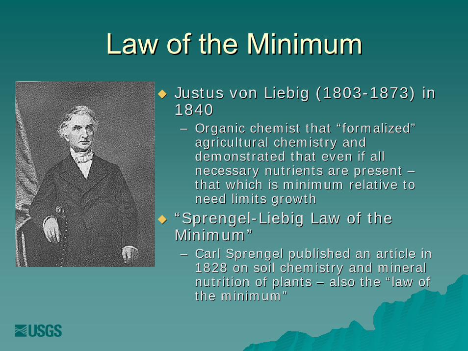
Law of the MinimumLaw of the MinimumJustus von Liebig (1803Justus von Liebig (1803--1873) in 1873) in 18401840–– Organic chemist that “formalized” Organic chemist that “formalized”

agricultural chemistry and agricultural chemistry and demonstrated that even if all demonstrated that even if all necessary nutrients are present necessary nutrients are present ––that which is minimum relative to that which is minimum relative to need limits growthneed limits growth

““SprengelSprengel--Liebig Law of the Liebig Law of the Minimum”Minimum”–– Carl Carl SprengelSprengel published an article in published an article in

1828 on soil chemistry and mineral 1828 on soil chemistry and mineral nutrition of plants nutrition of plants –– also the “law of also the “law of the minimum”the minimum”

Law of Law of ToleranceTolerance

F.E. Blackman, a plant physiologist, noted that F.E. Blackman, a plant physiologist, noted that too much as well as too little could also limit too much as well as too little could also limit growth.growth.–– ““When a process is conditioned as to its rapidity by a When a process is conditioned as to its rapidity by a

number of separate factors, the rate of the process is number of separate factors, the rate of the process is limited by the pace of the slowest factor.” from limited by the pace of the slowest factor.” from Blackman (1905) Ann. Blackman (1905) Ann. BotBot. 19, 281. 19, 281

V.E. V.E. ShelfordShelford (1913) proposed a more general (1913) proposed a more general concept concept -- “The Law of Tolerance”“The Law of Tolerance”–– SurvivorshipSurvivorship–– Growth and reproductionGrowth and reproduction–– Geographical and ecological distributionGeographical and ecological distribution

Polygonal DistributionsPolygonal DistributionsObservation and approachObservation and approach

Thomson et al. 1996

Polygonal RelationshipsPolygonal Relationships

Predator length Body size

Prey

leng

th

Abu

ndan

ce

Scarf et al. 1998

Is Simple Linear Regression Is Simple Linear Regression Ecologically Realistic?Ecologically Realistic?

RegressionGrowth rate = -0.6411+0.7181*x

1 2 3 4 5 6 7 8 9 10 11Food density

-2

0

2

46

8

1012

Gro

wth

rate

R2 = 0.40, p<< 0.001

Thomson et al. 1996Blackburn et al. 1992


Working with vs. ignoring limiting factors

1 2 3 4 5 6 7 8 9 10 11Food density

-2

0

2

4

6

8

10

12

Gro

wth

rate


1 2 3 4 5 6 7 8 9 10 11Food density

-2

0

2

46

8

1012

Gro

wth

rate

R2 = 0.40, p<< 0.001



Working with vs. ignoring limiting factors

1 2 3 4 5 6 7 8 9 10 11Food density

-2

0

2

4

6

8

10

12

Gro

wth

rate

Factors that decreaseoptimal growth rate


1 2 3 4 5 6 7 8 9 10 11Food density

-2

0

2

46

8

1012

Gro

wth

rate

R2 = 0.40, p<< 0.001


Examples From Impact Examples From Impact AssessmentsAssessments

These relationships are often These relationships are often observed in impact assessments ...observed in impact assessments ...

Santa Clara ValleySanta Clara ValleyWorking within the constraints of an urban environmentWorking within the constraints of an urban environment

EPT richness = 19.1 - 0.11 (inter-site road density) p << 0.001, r2 = 0.24

0 20 40 60 80 100 120 140Inter-site road density

0

5

10

15

20

25

30

EP

T ric

hnes

s

Figure 1. A map of the United States showing the location of the three study regionsand sampling sites: Mid-Atlantic (Baltimore, Maryland), Midwest (Cleveland, Ohio), and Pacific Coast (San Jose, California).

Alison Purcell O’Dowd and others, In review.

LargeLarge--scale Urban Studyscale Urban Study

Figure 2. Example of scatterplots showing a biological index (Y-Axis) plotted against an urban gradient (X-Axis). The plot on the left shows an example of a linear regression line (r2 = 0.19), while the plot on the right shows an example of a 95% quantile regression line to better characterize the upper boundary of the wedge-shaped plot.

Alison Purcell O’Dowd and others, In review.

LargeLarge--scale Agriculturescale Agriculture(upper mid(upper mid--west)west)

Julie Berkman and others, In review.

Upper MidUpper Mid--west Ag Studywest Ag StudyEPT density = 224.2 + 44.0 (% row crops)

0 20 40 60 80 100% of row crop in subbasin

0

2000

4000

6000

8000

10000

12000

14000

16000

18000E

PT

dens

ity (i

ndiv

idua

ls m

-2)

Julie Berkman and others, In review.

SmallSmall--scale “Single Stressor” Studyscale “Single Stressor” Study

Figure 1. Santa Clara Valley Area showing site locations. ● are sites on non-regulated streams, ▲ are sites on regulated streams.

EPT m-2 = 571.1 - 14.1 (grams fine sediment)

0 5 10 15 20 25 30 35 40 45 50Fine sediment per sample (grams)

0

200

400

600

800

1000

1200

1400

1600

EP

T de

nsity

(ind

ivid

uals

m-2

)

EPT richness = 8.7 - 0.2 (grams fine sediment)

0 5 10 15 20 25 30 35 40 45 50Fine sediment per sample (grams)

0

2

4

6

8

10

12

14

EP

T ric

hnes

s

Janny Choy and friends

SF Bay contaminantsSF Bay contaminants

Bivalve condition vs. silver contamination

0.0 0.2 0.4 0.6 0.8 1.0 1.2 1.4 1.6 1.8 2.0Contaminant (log[Ag])

5

10

15

20

25

30

35

40

45

Con

ditio

n in

dex

Cindy Brown and others, In prep

Corbula amurensis

Methods for Estimating Methods for Estimating The CeilingsThe Ceilings

AndAndSome Possible Some Possible ApplicationsApplications

Two Proposed MethodsTwo Proposed Methods

Partitioned Partitioned regressionregression–– Simple regression Simple regression

defines two groups defines two groups based on the sign of based on the sign of the residualthe residual

–– Iterate the above to Iterate the above to produce more produce more groups and identify groups and identify a ceilinga ceiling

QuantileQuantile regressionregression–– Group on the Group on the

independent independent variable (e.g., variable (e.g., classing by ~ equal classing by ~ equal n, effectn, effect--level, etc.)level, etc.)

–– Regress on a chosen Regress on a chosen percentile to percentile to establish a ceiling … establish a ceiling … or or

–– Weighted regressionWeighted regression

Koenker 2000 and earlier;Scharf et al. 1998; Cade 1999

Thomson et al. 1996

Our Polygonal DistributionOur Polygonal DistributionInter-site road density v. EPT richness


0

5

10

15

20

25

30E

PT

richn

ess

RegressRegressInter-site road density v. EPT richness


0

5

10

15

20

25

30E

PT

richn

ess

r2 = 0.24; r = -0.49, p << 0.001

Partitioned by ResidualsPartitioned by ResidualsInter-site road density v. EPT richness


0

5

10

15

20

25

30E

PT

richn

ess

residual > 0 residual < 0

r2 = 0.24; r = -0.49, p << 0.001

Inter-site road density v. EPT richness


0

5

10

15

20

25

30

EP

T ric

hnes

s

residual > 0 residual < 0

r2 = 0.24; r = -0.49, p << 0.001

Regress and Partition AgainRegress and Partition AgainResiduals > 0


0

5

10

15

20

25

30

EP

T ric

hnes

s

r2 = 0.53; r = -0.73, p << 0.001

Residuals < 0


0

5

10

15

20

25

30

EP

T ric

hnes

s

r2 = 0.30; r = -0.55, p << 0.001

Identifying the CeilingIdentifying the Ceiling= maximum current biological potential= maximum current biological potential

per unit urbanizationper unit urbanizationIdentifying the ceiling


0

5

10

15

20

25

30

EP

T ric

hnes

s

first residual <0 second residual <0 second residual >0

QuantileQuantile RegressionRegressionvia via ScharfScharf –– but see but see KoenkerKoenker / Cade / others/ Cade / others

Inter-site road density v. EPT richness


0

5

10

15

20

25

30E

PT

richn

ess

75th Percentile

http://www.fort.usgs.gov/Products/Software/blossom/

Cade, B.S., and J.D. Richards. 2005. User manual for Blossom statistical software. Fort Collins, CO: U.S. Geological Survey, Fort Collins Science Center. Open-File Report 2005-1353. 124 p.

Cade, B. S., and B. R. Noon. 2003. A gentle introduction to quantile regression for ecologists. Front Ecol Environ 1(8): 412-420.

QuantileQuantile RegressionRegression

Extending the TechniqueExtending the Technique

0.0 0.2 0.4 0.6 0.8 1.0 1.2 1.4 1.6% Urban (transformed)

0

1

2

3

4

5

6

7

8

9B

iotic

inde

x

"Unimpaired" Slightly impaired Impaired Trashed

In SummaryIn SummaryThere is an upper limit to stream quality in There is an upper limit to stream quality in practically any practically any anthropogenicallyanthropogenically influenced area.influenced area.–– This limit is set by existing and historic land cover and This limit is set by existing and historic land cover and

land use.land use.Even if mitigation occurs via Even if mitigation occurs via BMPsBMPs and and restoration, it’s likely that some anthropogenic restoration, it’s likely that some anthropogenic influences will not be totally eliminatedinfluences will not be totally eliminated–– e.g., urban impervious surface, agricultural land usee.g., urban impervious surface, agricultural land use

Therefore, it’s prudent to account for these Therefore, it’s prudent to account for these influences, which are often in the form of influences, which are often in the form of gradients, in the process of establishing realistic gradients, in the process of establishing realistic (i.e., attainable) reference conditions(i.e., attainable) reference conditions–– Which we defined as the maximum biological potential of Which we defined as the maximum biological potential of

a site.a site.

In SummaryIn SummaryThere is an upper limit to stream quality in There is an upper limit to stream quality in practically any practically any anthropogenicallyanthropogenically influenced area.influenced area.–– This limit is set by existing and historic land cover and This limit is set by existing and historic land cover and

land use.land use.Even if mitigation occurs via Even if mitigation occurs via BMPsBMPs and and restoration, it’s likely that some anthropogenic restoration, it’s likely that some anthropogenic influences will not be totally eliminatedinfluences will not be totally eliminated–– e.g., urban impervious surface, agricultural land usee.g., urban impervious surface, agricultural land use

Therefore, it’s prudent to account for these Therefore, it’s prudent to account for these influences, which are often in the form of influences, which are often in the form of gradients, in the process of establishing realistic gradients, in the process of establishing realistic (i.e., attainable) reference conditions(i.e., attainable) reference conditions–– Defined as the maximum biological potential of a site as Defined as the maximum biological potential of a site as

set by a factorset by a factor--ceiling.ceiling.

In questions of sciences, the In questions of sciences, the authority of a thousand is not authority of a thousand is not

worth the humble reasoning of a worth the humble reasoning of a single individual.single individual.

GalileoGalileo

The world is composed of The world is composed of gradients not boxes gradients not boxes ––

we’ve probably ignored them for we’ve probably ignored them for too long.too long.

Factor-ceilings - California

Documents

Transcript of Factor-ceilings - California