Face Image Analysis With Convolutional Neural Networks · Face Image Analysis With Convolutional...
191
Face Image Analysis With Convolutional Neural Networks Dissertation Zur Erlangung des Doktorgrades der Fakult¨at f¨ ur Angewandte Wissenschaften an der Albert-Ludwigs-Universit¨at Freiburg im Breisgau von Stefan Duffner 2007
Transcript of Face Image Analysis With Convolutional Neural Networks · Face Image Analysis With Convolutional...
Face Image Analysis With
Convolutional Neural Networks
Dissertation
Zur Erlangung des Doktorgrades
der Fakultat fur Angewandte Wissenschaften
an der Albert-Ludwigs-Universitat Freiburg im Breisgau
von
Stefan Duffner
2007

Dekan: Prof. Dr. Bernhard Nebel
Prufungskommission: Prof. Dr. Peter Thiemann (Vorsitz)Prof. Dr. Matthias Teschner (Beisitz)Prof. Dr. Hans Burkhardt (Betreuer)Prof. Dr. Thomas Vetter (Prufer)
Datum der Disputation: 28. Marz 2008

Acknowledgments
First of all, I would like to thank Dr. Christophe Garcia for his guidance andsupport over the last three years. This work would not have been possiblewithout his excellent scientific as well as human qualities and the enormousamount of time he spent for me.
I also want to express my gratitude to my supervisor Prof. Dr. Hans Burk-hardt who accompanied me during my thesis, gave me helpful advice and whoalways welcomed me in Freiburg.
Further, I would like to thank all my colleagues at France Telecom R&D(now Orange Labs), Rennes (France) where I spent three very pleasant years.Notably, Franck Mamalet, Sebastien Roux, Patrick Lechat, Sid-Ahmed Berrani,Zohra Saidane, Muriel Visani, Antoine Lehuger, Gregoire Lefebvre, ManolisDelakis and Christine Barbot.
Finally, I want to say thank you to my parents for their continuing supportin every respect.
ii
Abstract
In this work, we present the problem of automatic appearance-based facialanalysis with machine learning techniques and describe common specific sub-problems like face detection, facial feature detection and face recognition whichare the crucial parts of many applications in the context of indexation, surveil-lance, access-control or human-computer interaction.
To tackle this problem, we particularly focus on a technique called Convolu-tional Neural Network (CNN) which is inspired by biological evidence found inthe visual cortex of mammalian brains and which has already been applied tomany different classification problems. Existing CNN-based methods, like theface detection system proposed by Garcia and Delakis, show that this can bea very effective, efficient and robust approach to non-linear image processingtasks such as facial analysis.
An important step in many automatic facial analysis applications, e.g. facerecognition, is face alignment which tries to translate, scale and rotate the faceimage such that specific facial features are roughly at predefined positions inthe image. We propose an efficient approach to this problem using CNNs andexperimentally show its very good performance on difficult test images.
We further present a CNN-based method for automatic facial feature detec-tion. The proposed system employs a hierarchical procedure which first roughlylocalizes the eyes, the nose and the mouth and then refines the result by detect-ing 10 different facial feature points. The detection rate of this method is 96%for the AR database and 87% for the BioID database tolerating an error of 10%of the inter-ocular distance.
Finally, we propose a novel face recognition approach based on a specificCNN architecture learning a non-linear mapping of the image space into a lower-dimensional sub-space where the different classes are more easily separable.We applied this method to several public face databases and obtained betterrecognition rates than with classical face recognition approaches based on PCAor LDA. Moreover, the proposed system is particularly robust to noise andpartial occlusions.
We also present a CNN-based method for the binary classification problemof gender recognition with face images and achieve a state-of-the-art accuracy.
The results presented in this work show that CNNs perform very well onvarious facial image processing tasks, such as face alignment, facial feature de-tection and face recognition and clearly demonstrate that the CNN techniqueis a versatile, efficient and robust approach for facial image analysis.
iii
Zusammenfassung
In dieser Arbeit stellen wir das Problem der automatischen, erscheinungsbasier-ten Gesichts-Analyse dar und beschreiben gangige, spezifische Unterproblemewie z.B. Gesichts- und Gesichtsmerkmals-Lokalisierung oder Gesichtserkennung,welche grundlegende Bestandteile vieler Anwendungen im Bereich Indexierung,Uberwachung, Zugangskontrolle oder Mensch-Maschine-Interaktion sind.
Um dieses Problem anzugehen, konzentrieren wir uns auf einen bestimmtenAnsatz, genannt Neuronales Faltungs-Netzwerk, englisch Convolutional NeuralNetwork (CNN), welcher auf biologischen Befunden, die im visuellen Kortex vonSaugetierhirnen entdeckt wurden, beruht und welcher bereits auf viele Klassifi-zierungsprobleme angewandt wurde. Bestehende CNN-basierte Methoden, wiedas Gesichts-Lokalisierungs-System von Garcia und Delakis, zeigen, dass diesein sehr effektiver, effizienter und robuster Ansatz fur nicht-lineare Bildverar-beitungs-Aufgaben wie Gesichts-Analyse sein kann.
Ein wichtiger Schritt in vielen Anwendungen der automatischen Gesichts-Analyse, z.B. Gesichtserkennung, ist die Gesichts-Ausrichtung und -Zentrierung.Diese versucht das Gesichts-Bild so zu verschieben, zu drehen und zu vergroßernbzw. verkleinern, dass sich bestimmte Gesichtsmerkmale an vordefinierten Bild-Positionen befinden. Wir stellen einen effizienten Ansatz fur dieses Problemvor, der auf CNNs beruht, und zeigen experimentell und anhand schwierigerTestbilder die sehr gute Leistungsfahigkeit des Systems.
Daruberhinaus stellen wir eine CNN-basierte Methode zur automatischenGesichtsmerkmals-Lokalisierung vor. Das System bedient sich einem hierarchi-schen Verfahren, das zuerst grob die Augen, die Nase und den Mund lokalisiert,und dann das Ergebnis verfeinert indem es 10 verschiedene Gesichtsmerkmals-Punkte erkennt. Die Erkennungsrate dieser Methode liegt bei 96% fur die AR-Datenbank und 87% fur die BioID-Datenbank mit einer Fehler-Toleranz von10% des Augenabstandes.
Schließlich stellen wir einen neuen Gesichtserkennungs-Ansatz vor, welcherauf einer spezifischen CNN-Architektur beruht und welcher eine nicht-lineareAbbildung vom Bildraum in einen niedrig-dimensionalen Unterraum lernt, indem die verschiedenen Klassen leichter trennbar sind. Diese Methode wurdeauf verschiedene offentliche Gesichts-Datenbanken angewandt und erzielte bes-sere Erkennungsraten als klassische Gesichtserkennungs-Ansatze, die auf PCAoder LDA beruhen. Daruberhinaus ist das System besonders robust bezuglichRauschen und partiellen Verdeckungen.
Wir stellen ferner eine CNN-basierte Methode zum binaren Klassifizierung-Problem der Geschlechtserkennung mittels Gesichts-Bildern vor und erzieleneine Genauigkeit, die dem aktuellen Stand der Technik entspricht.
Die Ergebnisse, die in dieser Arbeit dargestellt sind, beweisen, dass CNNssehr gute Leistungen in verschiedenen Gesichts-Bildverarbeitungs-Aufgaben er-zielen, wie z.B. Gesichts-Ausrichtung, Gesichtsmerkmals-Lokalisierung und Ge-sichtserkennung. Sie zeigen außerdem deutlich, dass CNNs ein vielseitiges, effi-zientes und robustes Verfahren zur Gesichts-Analyse sind.
iv

Resume
Dans cette these, nous proposons le probleme de l’analyse faciale basee surl’apparence avec des techniques d’apprentissage automatique et nous decrivonsdes sous-problemes specifiques tels que la detection de visage, la detection decaracteristiques faciales et la reconnaissance de visage qui sont des composantsindispensables dans de nombreuses applications dans le contexte de l’indexation,la surveillance, le controle d’acces et l’interaction homme-machine.
Afin d’aborder ce probleme, nous nous concentrons sur une technique nommeereseau de neurones a convolution, en anglais Convolutional Neural Network(CNN), qui est inspiree des decouvertes biologiques dans le cortex visuel desmammiferes et qui a deja ete appliquee a de nombreux problemes de classifica-tion. Des methodes existantes, comme le systeme de detection de visage proposepar Garcia et Delakis, montrent que cela peut etre une approche tres efficaceet robuste pour des applications de traitement non-lineaire d’images tel quel’analyse faciale.
Une etape importante dans beaucoup d’applications d’analyse facial, commela reconnaissance de visage, constitue le recadrage automatique de visage. Cettetechnique cherche a decaler, tourner et agrandir ou reduire l’image de visagede sorte que des caracteristiques faciales se trouvent environ a des positionsdefinies prealablement dans l’image. Nous proposons une approche efficace pource probleme en utilisant des CNNs et nous montrons une tres bonne performancede cette approche sur des images de test difficiles.
Nous presentons egalement une methode basee CNN pour la detection decaracteristiques faciales. Le systeme propose utilise une procedure hierarchiquequi localise d’abord les yeux, le nez et la bouche pour ensuite affiner le resultat endetectant 10 points de caracteristiques faciales differentes. Le taux de detectionest de 96 % pour la base AR et de 87 % pour la base BioID avec une toleranced’erreur de 10 % de la distance inter-oculaire.
Enfin, nous proposons une nouvelle approche de reconnaissance de visagebasee sur une architecture specifique de CNN qui apprend une projection non-lineaire de l’espace de l’image dans un espace de dimension reduite ou les classesdifferentes sont separables plus facilement. Nous appliquons cette methode aplusieurs bases publiques de visage et nous obtenons des taux de reconnais-sance meilleurs qu’en utilisant des approches classiques basees sur l’Analyse enComposantes Principales (ACP) ou l’Analyse Discriminante Lineaire (ADL).En outre, le systeme propose est particulierement robuste par rapport au bruitet aux occultations partielles.
Nous presentons egalement une methode basee CNN pour le probleme dereconnaissance de genre a partir d’images de visage et nous obtenons un tauxcomparable a l’etat de l’art.
Les resultats presentes dans cette these montrent que les CNNs sont tresperformants dans de nombreuses applications de traitement d’images facialestelles que le recadrage de visage, la detection de caracteristiques faciales et lareconnaissance de visage. Ils demontrent egalement que la technique de CNN estune approche tres variee, efficace et robuste pour l’analyse automatique d’imagefaciale.
v

Contents
1 Introduction 1
1.1 Context . . . . . . . . . . . . . . . . . . . . . . . . . . . . . . . . 11.2 Applications . . . . . . . . . . . . . . . . . . . . . . . . . . . . . . 21.3 Difficulties . . . . . . . . . . . . . . . . . . . . . . . . . . . . . . . 3
1.3.1 Illumination . . . . . . . . . . . . . . . . . . . . . . . . . . 31.3.2 Pose . . . . . . . . . . . . . . . . . . . . . . . . . . . . . . 41.3.3 Facial Expressions . . . . . . . . . . . . . . . . . . . . . . 41.3.4 Partial Occlusions . . . . . . . . . . . . . . . . . . . . . . 51.3.5 Other types of variations . . . . . . . . . . . . . . . . . . 5
1.4 Objectives . . . . . . . . . . . . . . . . . . . . . . . . . . . . . . . 51.5 Outline . . . . . . . . . . . . . . . . . . . . . . . . . . . . . . . . 6
2 Machine Learning Techniques for Object Detection and Recog-
nition 7
2.1 Introduction . . . . . . . . . . . . . . . . . . . . . . . . . . . . . . 72.2 Statistical Projection Methods . . . . . . . . . . . . . . . . . . . 8
2.2.1 Principal Component Analysis . . . . . . . . . . . . . . . 92.2.2 Linear Discriminant Analysis . . . . . . . . . . . . . . . . 102.2.3 Other Projection Methods . . . . . . . . . . . . . . . . . . 11
2.3 Active Appearance Models . . . . . . . . . . . . . . . . . . . . . 122.3.1 Modeling shape and appearance . . . . . . . . . . . . . . 122.3.2 Matching the model . . . . . . . . . . . . . . . . . . . . . 13
2.4 Hidden Markov Models . . . . . . . . . . . . . . . . . . . . . . . 142.4.1 Introduction . . . . . . . . . . . . . . . . . . . . . . . . . 142.4.2 Finding the most likely state sequence . . . . . . . . . . . 152.4.3 Training . . . . . . . . . . . . . . . . . . . . . . . . . . . . 162.4.4 HMMs for Image Analysis . . . . . . . . . . . . . . . . . . 16
2.5 Adaboost . . . . . . . . . . . . . . . . . . . . . . . . . . . . . . . 182.5.1 Introduction . . . . . . . . . . . . . . . . . . . . . . . . . 182.5.2 Training . . . . . . . . . . . . . . . . . . . . . . . . . . . . 18
2.6 Support Vector Machines . . . . . . . . . . . . . . . . . . . . . . 192.6.1 Structural Risk Minimization . . . . . . . . . . . . . . . . 192.6.2 Linear Support Vector Machines . . . . . . . . . . . . . . 202.6.3 Non-linear Support Vector Machines . . . . . . . . . . . . 212.6.4 Extension to multiple classes . . . . . . . . . . . . . . . . 22
2.7 Bag of Local Signatures . . . . . . . . . . . . . . . . . . . . . . . 222.8 Neural Networks . . . . . . . . . . . . . . . . . . . . . . . . . . . 24
2.8.1 Introduction . . . . . . . . . . . . . . . . . . . . . . . . . 24
vi

CONTENTS
2.8.2 Perceptron . . . . . . . . . . . . . . . . . . . . . . . . . . 242.8.3 Multi-Layer Perceptron . . . . . . . . . . . . . . . . . . . 252.8.4 Auto-Associative Neural Networks . . . . . . . . . . . . . 262.8.5 Training Neural Networks . . . . . . . . . . . . . . . . . . 272.8.6 Radial Basis Function Networks . . . . . . . . . . . . . . 402.8.7 Self-Organizing Maps . . . . . . . . . . . . . . . . . . . . 42
2.9 Conclusion . . . . . . . . . . . . . . . . . . . . . . . . . . . . . . 44
3 Convolutional Neural Networks 47
3.1 Introduction . . . . . . . . . . . . . . . . . . . . . . . . . . . . . . 473.2 Background . . . . . . . . . . . . . . . . . . . . . . . . . . . . . . 48
3.2.1 Neocognitron . . . . . . . . . . . . . . . . . . . . . . . . . 483.2.2 LeCun’s Convolutional Neural Network model . . . . . . . 50
3.3 Training Convolutional Neural Networks . . . . . . . . . . . . . . 533.3.1 Error Backpropagation with Convolutional Neural Networks 533.3.2 Other training algorithms proposed in the literature . . . 56
3.4 Extensions and variants . . . . . . . . . . . . . . . . . . . . . . . 593.4.1 LeNet-5 . . . . . . . . . . . . . . . . . . . . . . . . . . . . 593.4.2 Space Displacement Neural Networks . . . . . . . . . . . 603.4.3 Siamese CNNs . . . . . . . . . . . . . . . . . . . . . . . . 613.4.4 Shunting Inhibitory Convolutional Neural Networks . . . 643.4.5 Sparse Convolutional Neural Networks . . . . . . . . . . . 67
3.5 Some Applications . . . . . . . . . . . . . . . . . . . . . . . . . . 693.6 Conclusion . . . . . . . . . . . . . . . . . . . . . . . . . . . . . . 70
4 Face detection and normalization 71
4.1 Introduction . . . . . . . . . . . . . . . . . . . . . . . . . . . . . . 714.2 Face detection . . . . . . . . . . . . . . . . . . . . . . . . . . . . . 72
4.2.1 Introduction . . . . . . . . . . . . . . . . . . . . . . . . . 724.2.2 State-of-the-art . . . . . . . . . . . . . . . . . . . . . . . . 724.2.3 Convolutional Face Finder . . . . . . . . . . . . . . . . . . 75
4.3 Illumination Normalization . . . . . . . . . . . . . . . . . . . . . 824.4 Pose Estimation . . . . . . . . . . . . . . . . . . . . . . . . . . . 834.5 Face Alignment . . . . . . . . . . . . . . . . . . . . . . . . . . . . 86
4.5.1 Introduction . . . . . . . . . . . . . . . . . . . . . . . . . 864.5.2 State-of-the-art . . . . . . . . . . . . . . . . . . . . . . . . 874.5.3 Face Alignment with Convolutional Neural Networks . . . 88
4.6 Conclusion . . . . . . . . . . . . . . . . . . . . . . . . . . . . . . 95
5 Facial Feature Detection 98
5.1 Introduction . . . . . . . . . . . . . . . . . . . . . . . . . . . . . . 985.2 State-of-the-art . . . . . . . . . . . . . . . . . . . . . . . . . . . . 995.3 Facial Feature Detection with Convolutional Neural Networks . . 103
5.3.1 Introduction . . . . . . . . . . . . . . . . . . . . . . . . . 1035.3.2 Architecture of the Facial Feature Detection System . . . 1035.3.3 Training the Facial Feature Detectors . . . . . . . . . . . 1075.3.4 Facial Feature Detection Procedure . . . . . . . . . . . . . 1095.3.5 Experimental Results . . . . . . . . . . . . . . . . . . . . 109
5.4 Conclusion . . . . . . . . . . . . . . . . . . . . . . . . . . . . . . 120
vii

CONTENTS
6 Face and Gender Recognition 121
6.1 Introduction . . . . . . . . . . . . . . . . . . . . . . . . . . . . . . 1216.2 State-of-the-art in Face Recognition . . . . . . . . . . . . . . . . 1226.3 Face Recognition with Convolutional Neural Networks . . . . . . 125
6.3.1 Introduction . . . . . . . . . . . . . . . . . . . . . . . . . 1256.3.2 Neural Network Architecture . . . . . . . . . . . . . . . . 1266.3.3 Training Procedure . . . . . . . . . . . . . . . . . . . . . . 1276.3.4 Recognizing Faces . . . . . . . . . . . . . . . . . . . . . . 1296.3.5 Experimental Results . . . . . . . . . . . . . . . . . . . . 129
6.4 Gender Recognition . . . . . . . . . . . . . . . . . . . . . . . . . 1336.4.1 Introduction . . . . . . . . . . . . . . . . . . . . . . . . . 1336.4.2 State-of-the-art . . . . . . . . . . . . . . . . . . . . . . . . 1346.4.3 Gender Recognition with Convolutional Neural Networks 136
6.5 Conclusion . . . . . . . . . . . . . . . . . . . . . . . . . . . . . . 136
7 Conclusion and Perspectives 138
7.1 Conclusion . . . . . . . . . . . . . . . . . . . . . . . . . . . . . . 1387.2 Perspectives . . . . . . . . . . . . . . . . . . . . . . . . . . . . . . 140
7.2.1 Convolutional Neural Networks . . . . . . . . . . . . . . . 1407.2.2 Facial analysis with Convolutional Neural Networks . . . 140
A Excerpts from the used face databases 142
A.1 AR . . . . . . . . . . . . . . . . . . . . . . . . . . . . . . . . . . . 142A.2 BioID . . . . . . . . . . . . . . . . . . . . . . . . . . . . . . . . . 144A.3 FERET . . . . . . . . . . . . . . . . . . . . . . . . . . . . . . . . 146A.4 Google Images . . . . . . . . . . . . . . . . . . . . . . . . . . . . 148A.5 ORL . . . . . . . . . . . . . . . . . . . . . . . . . . . . . . . . . . 150A.6 PIE . . . . . . . . . . . . . . . . . . . . . . . . . . . . . . . . . . 152A.7 Yale . . . . . . . . . . . . . . . . . . . . . . . . . . . . . . . . . . 154
viii
List of Figures
1.1 An example face under a fixed view and varying illumination . . 31.2 An example face under fixed illumination and varying pose . . . 41.3 An example face under fixed illumination and pose but varying
facial expression . . . . . . . . . . . . . . . . . . . . . . . . . . . 4
2.1 Active Appearance Models: annotated training example and cor-responding shape-free patch . . . . . . . . . . . . . . . . . . . . . 13
2.2 A left-right Hidden Markov Model . . . . . . . . . . . . . . . . . 152.3 Two simple approaches to image analysis with 1D HMMs . . . . 172.4 Illustration of a 2D Pseudo-HMM . . . . . . . . . . . . . . . . . . 172.5 Graphical illustration of a linear SVM . . . . . . . . . . . . . . . 212.6 The histogram creation procedure with the Bag-of-local-signature
approach . . . . . . . . . . . . . . . . . . . . . . . . . . . . . . . . 232.7 The Perceptron . . . . . . . . . . . . . . . . . . . . . . . . . . . . 242.8 A Multi-Layer Perceptron . . . . . . . . . . . . . . . . . . . . . . 252.9 Different types of activation functions . . . . . . . . . . . . . . . 262.10 Auto-Associative Neural Networks . . . . . . . . . . . . . . . . . 262.11 Typical evolution of training and validation error . . . . . . . . . 312.12 The two possible cases that can occur when the minimum on the
validation set is reached . . . . . . . . . . . . . . . . . . . . . . . 342.13 A typical evolution of the error criteria on the validation set using
the proposed learning algorithm . . . . . . . . . . . . . . . . . . . 362.14 The evolution of the validation error on the NIST database using
Backpropagation and the proposed algorithm . . . . . . . . . . . 372.15 The validation error curves of the proposed approach with differ-
ent initial global learning rates . . . . . . . . . . . . . . . . . . . 372.16 The architecture of a RBF Network . . . . . . . . . . . . . . . . 412.17 A two-dimensional SOM with rectangular topology . . . . . . . . 432.18 Evolution of a two-dimensional SOM during training . . . . . . . 45
3.1 The model of a S-cell used in the Neocognitron . . . . . . . . . . 483.2 The topology of the basic Neocognitron . . . . . . . . . . . . . . 503.3 Some training examples used to train the first two S-layers of
Fukushima’s Neocognitron . . . . . . . . . . . . . . . . . . . . . . 513.4 The architecture of LeNet-1 . . . . . . . . . . . . . . . . . . . . . 523.5 Convolution and sub-sampling . . . . . . . . . . . . . . . . . . . 523.6 Error Backpropagation with convolution maps . . . . . . . . . . 553.7 Error Backpropagation with sub-sampling maps . . . . . . . . . . 55
ix
LIST OF FIGURES
3.8 The architecture of LeNet-5 . . . . . . . . . . . . . . . . . . . . . 593.9 A Space Displacement Neural Network . . . . . . . . . . . . . . . 613.10 Illustration of a Siamese Convolutional Neural Network . . . . . 623.11 Example of positive (genuine) and negative (impostor) error func-
tions for Siamese CNNs . . . . . . . . . . . . . . . . . . . . . . . 633.12 The shunting inhibitory neuron model . . . . . . . . . . . . . . . 653.13 The SICoNNet architecture . . . . . . . . . . . . . . . . . . . . . 663.14 The connection scheme of the SCNN proposed by Gepperth . . . 673.15 The sparse, shift-invariant CNN model proposed by Ranzato et al . 68
4.1 The architecture of the Convolutional Face Finder . . . . . . . . 764.2 Training examples for the Convolutional Face Finder . . . . . . . 774.3 The face localization procedure of the Convolutional Face Finder 784.4 Convolutional Face Finder: ROC curves for different test sets . . 804.5 Some face detection results of the Convolutional Face Finder ob-
tained with the CMU test set . . . . . . . . . . . . . . . . . . . . 814.6 The three rotation axes defined with respect to a frontal head . . 844.7 The face alignment process of the proposed approach . . . . . . . 874.8 The Neural Network architecture of the proposed face alignment
system . . . . . . . . . . . . . . . . . . . . . . . . . . . . . . . . . 894.9 Training examples for the proposed face alignment system . . . . 904.10 The overall face alignment procedure of the proposed system . . 914.11 Correct alignment rate vs. allowed mean corner distance of the
proposed approach . . . . . . . . . . . . . . . . . . . . . . . . . . 934.12 Precision of the proposed alignment approach and the approach
based on facial feature detection . . . . . . . . . . . . . . . . . . 934.13 Sensitivity analysis of the proposed alignment approach: Gaus-
sian noise . . . . . . . . . . . . . . . . . . . . . . . . . . . . . . . 944.14 Sensitivity analysis of the proposed alignment approach: partial
occlusion . . . . . . . . . . . . . . . . . . . . . . . . . . . . . . . 954.15 Some face alignment results of the proposed approach on the
Internet test set . . . . . . . . . . . . . . . . . . . . . . . . . . . . 96
5.1 Principal stages of the feature detection process of the proposedapproach . . . . . . . . . . . . . . . . . . . . . . . . . . . . . . . . 104
5.2 Some input images and corresponding desired output feature maps1055.3 Architecture of the proposed facial feature detector . . . . . . . . 1065.4 Eye feature detector: example of an input image with desired
facial feature points, desired output maps and superposed desiredoutput maps . . . . . . . . . . . . . . . . . . . . . . . . . . . . . 107
5.5 Mouth feature detector: example of an input image with desiredfacial feature points, desired output maps and superposed desiredoutput maps . . . . . . . . . . . . . . . . . . . . . . . . . . . . . 107
5.6 Facial feature detector: virtual face images created by applyingvarious geometric transformations . . . . . . . . . . . . . . . . . . 108
5.7 Facial feature detector: detection rate versus me of the four features1105.8 Facial feature detector: detection rate versus mei of each facial
feature (FERET) . . . . . . . . . . . . . . . . . . . . . . . . . . . 1115.9 Facial feature detector: detection rate versus mei of each facial
feature (Google images) . . . . . . . . . . . . . . . . . . . . . . . 111
x

LIST OF FIGURES
5.10 Facial feature detector: detection rate versus mei of each facialfeature (PIE subset) . . . . . . . . . . . . . . . . . . . . . . . . . 112
5.11 The different types of CNN input features that have been tested 1135.12 ROC curves comparing the CNNs trained with different input
features (FERET database) . . . . . . . . . . . . . . . . . . . . . 1145.13 ROC curves comparing the CNNs trained with different input
features (Google images) . . . . . . . . . . . . . . . . . . . . . . . 1145.14 ROC curves comparing the CNNs trained with different input
features (PIE subset) . . . . . . . . . . . . . . . . . . . . . . . . . 1155.15 Sensitivity analysis of the proposed facial feature detector: Gaus-
sian noise . . . . . . . . . . . . . . . . . . . . . . . . . . . . . . . 1155.16 Sensitivity analysis of the proposed facial feature detector: partial
occlusion . . . . . . . . . . . . . . . . . . . . . . . . . . . . . . . 1165.17 Facial feature detection results on different face databases . . . . 1175.18 Overall detection rate of the proposed facial feature detection
method for AR . . . . . . . . . . . . . . . . . . . . . . . . . . . . 1175.19 Overall detection rate of the proposed facial feature detection
method for BioID . . . . . . . . . . . . . . . . . . . . . . . . . . . 1185.20 Some results of combined face and facial feature detection with
the proposed approach . . . . . . . . . . . . . . . . . . . . . . . . 119
6.1 The basic schema of our face recognition approach showing twodifferent individuals . . . . . . . . . . . . . . . . . . . . . . . . . 126
6.2 Architecture of the proposed Neural Network for face recognition 1276.3 ROC curves of the proposed face recognition algorithm for the
ORL and Yale databases . . . . . . . . . . . . . . . . . . . . . . . 1306.4 Examples of image reconstruction of the proposed face recogni-
tion approach . . . . . . . . . . . . . . . . . . . . . . . . . . . . . 1316.5 Comparison of the proposed approach with the Eigenfaces and
Fisherfaces approach: ORL database . . . . . . . . . . . . . . . . 1326.6 Comparison of the proposed approach with the Eigenfaces and
Fisherfaces approach: Yale database . . . . . . . . . . . . . . . . 1326.7 Sensitivity analysis of the proposed face recognition approach:
Gaussian noise . . . . . . . . . . . . . . . . . . . . . . . . . . . . 1336.8 Sensitivity analysis of the proposed face recognition approach:
partial occlusion . . . . . . . . . . . . . . . . . . . . . . . . . . . 1346.9 Examples of training images for gender classification . . . . . . . 1366.10 ROC curve of the gender recognition CNN applied to the unmixed
FERET test set . . . . . . . . . . . . . . . . . . . . . . . . . . . . 137
xi

List of Tables
2.1 Comparison of the proposed learning algorithm with Backpropa-gation and the bold driver method (10 hidden neurons) . . . . . 37
2.2 Comparison of the proposed learning algorithm with Backpropa-gation and the bold driver method (40 hidden neurons) . . . . . 38
3.1 The connection scheme of layer C3 of Lenet-5 . . . . . . . . . . . 60
4.1 Detection rate vs. false alarm rate of selected face detection meth-ods on the CMU test set. . . . . . . . . . . . . . . . . . . . . . . 75
4.2 The connection scheme of layer C2 of the Convolutional FaceFinder . . . . . . . . . . . . . . . . . . . . . . . . . . . . . . . . . 77
4.3 Comparison of face detection results evaluated on the CMU andMIT test sets . . . . . . . . . . . . . . . . . . . . . . . . . . . . . 81
4.4 Execution speed of the CFF on different platforms . . . . . . . . 81
5.1 Overview of detection rates of some published facial feature de-tection methods . . . . . . . . . . . . . . . . . . . . . . . . . . . . 102
5.2 Comparison of eye pupil detection rates of some published meth-ods on the BioID database . . . . . . . . . . . . . . . . . . . . . . 118
6.1 Recognition rates of the proposed approach compared to Eigen-faces and Fisherfaces . . . . . . . . . . . . . . . . . . . . . . . . . 131
xii

List of Algorithms
1 The Viterbi algorithm . . . . . . . . . . . . . . . . . . . . . . . . 162 The Adaboost algorithm . . . . . . . . . . . . . . . . . . . . . . . 193 The standard online Backpropagation algorithm for MLPs . . . . 304 The proposed online Backpropagation algorithm with adaptive
learning rate . . . . . . . . . . . . . . . . . . . . . . . . . . . . . 355 The RPROP algorithm . . . . . . . . . . . . . . . . . . . . . . . . 396 The line search algorithm . . . . . . . . . . . . . . . . . . . . . . 397 A training algorithm for Self-Organizing Maps . . . . . . . . . . 448 The online Backpropagation algorithm for Convolutional Neural
Networks . . . . . . . . . . . . . . . . . . . . . . . . . . . . . . . 57
xiii

Chapter 1
Introduction
1.1 Context
The automatic processing of images to extract semantic content is a task thathas gained a lot of importance during the last years due to the constantlyincreasing number of digital photographs on the Internet or being stored onpersonal home computers. The need to organize them automatically in a intel-ligent way using indexing and image retrieval techniques requires effective andefficient image analysis and pattern recognition algorithms that are capable toextract relevant semantic information.
Especially faces contain a great deal of valuable information compared toother objects or visual items in images. For example, recognizing a person on aphotograph, in general, tells a lot about the overall content of the picture.
In the context of human-computer interaction (HCI), it might also be im-portant to detect the position of specific facial characteristics or recognize facialexpressions, in order to allow, for example, a more intuitive communication be-tween the device and the user or to efficiently encode and transmit facial imagescoming from a camera. Thus, the automatic analysis of face images is crucialfor many applications involving visual content retrieval or extraction.
The principal aim of facial analysis is to extract valuable information fromface images, such as its position in the image, facial characteristics, facial ex-pressions, the person’s gender or identity.
We will outline the most important existing approaches to facial image anal-ysis and present novel methods based on Convolutional Neural Networks (CNN)to detect, normalize and recognize faces and facial features. CNNs show to be apowerful and flexible feature extraction and classification technique which hasbeen successfully applied in other contexts, i.e. hand-written character recogni-tion, and which is very appropriate for face analysis problems as we will exper-imentally show in this work.
We will focus on the processing of two-dimensional gray-level images as thisis the most widespread form of digital images and thus allows the proposedapproaches to be applied in the most extensive and generic way. However,many techniques described in this work could also be extended to color images,3D data or multi-modal data.
1

1.2. APPLICATIONS
1.2 Applications
There are numerous possible applications for facial image processing algorithms.The most important of them concern face recognition. In this regard, one hasto differentiate between closed world and open world settings. In a closed worldapplication, the algorithm is dedicated to a limited group of persons, e.g. torecognize the members of a family. In an open world context the algorithmshould be able to deal with images from “unknown” persons, i.e. persons thathave not been presented to the system during its design or training. For example,an application indexing large image databases like Google images or televisionprograms should recognize learned persons and respond with “unknown” if theperson is not in the database of registered persons.
Concerning face recognition, there further exist two types of problems: faceidentification and face verification (or authentication). The first problem, faceidentification, is to determine the identity of a person on an image. The secondone only deals with the question: “Is ‘X’ the identity of the person shown onthe image?” or “Is the person shown on the image the one he claims to be?”.These questions only require “yes” or “no” as the answer.
Possible applications for face authentication are mainly concerned with ac-cess control, e.g. restricting the physical access to a building, such as a corporatebuilding, a secured zone of an airport, a house etc. Instead of opening a doorby a key or a code, the respective person would communicate an identifier, e.g.his/her name, and present his/her face to a camera. The face authenticationsystem would then verify the identity of the person and grant or refuse theaccess accordingly. This principle could equally be applied to the access to sys-tems, automatic teller machines, mobile phones, Internet sites etc. where onewould present his face to a camera instead of entering an identification numberor password.
Clearly, also face identification can be used for controlling access. In thiscase the person only has to present his/her face to the camera without claiminghis/her identity. A system recognizing the identity of a person can further beemployed to control more specifically the rights of the respective persons storedin its database. For instance, parents could allow their children to watch onlycertain television programs or web sites, while the television or computer wouldautomatically recognize the persons in front of it.
Video surveillance is another application of face identification. The aim hereis to recognize suspects or criminals using video cameras installed at publicplaces, such as banks or airports, in order to increase the overall security ofthese places. In this context, the database of suspects to recognize is often verylarge and the images captured by the camera are of low quality, which makesthe task rather difficult.
With the vast propagation of digital cameras in the last years the numberof digital images stored on servers and personal home computers is rapidlygrowing. Consequently, there is an increasing need of indexation systems thatautomatically categorize and annotate this huge amount of images in orderto allow effective searching and so-called content-based image retrieval. Here,face detection and recognition methods play a crucial role because a great partof photographs actually contain faces. A similar application is the temporalsegmentation and indexation of video sequences, such as TV programs, wheredifferent scenes are often characterized by different faces.
2

CHAPTER 1. INTRODUCTION
Figure 1.1: An example face under a fixed view and varying illumination
Another field of application is facial image compression, i.e. parts of imagescontaining faces can be coded by a specialized algorithm that incorporates ageneric face model and thus leads to very high compression rates compared touniversal techniques.
Finally, there are many possible applications in the field of advanced Human-Computer Interaction (HCI), e.g. the control and animation of avatars, i.e. com-puter synthesized characters. Such systems capture the position and movementof the face and facial features and accordingly animate a virtual avatar, whichcan be seen by the interlocutor. Another example would be the facilitation ofthe interaction of disabled persons with computers or other machines or theautomatic recognition of facial expressions in order to detect the reaction of theperson(s) sitting in front of a camera (e.g. smiling, laughing, yawning, sleeping).
1.3 Difficulties
There are some inherent properties of faces as well as the way the images arecaptured which make the automatic processing of face images a rather difficulttask. In the case of face recognition, this leads to the problem that the intra-classvariance, i.e. variations of the face of the same person due to lighting, pose etc.,is often higher than the inter-class variance, i.e. variations of facial appearanceof different persons, and thus reduces the recognition rate. In many face analysisapplications, the appearance variation resulting from these circumstances canalso be considered as noise as it makes the desired information, i.e. the identityof the person, harder to extract and reduces the overall performance of therespective systems.
In the following, we will outline the most important difficulties encounteredin common real-world applications.
1.3.1 Illumination
Changes in illumination can entail considerable variations of the appearance offaces and thus face images. Two main types of light sources influence the overallillumination: ambient light and point light (or directed light). The former issomehow easier to handle because it only affects the overall brightness of theresulting image. The latter however is far more difficult to analyze, as faceimages taken under varying light source directions follow a highly non-linearfunction. Additionally, the face can cast shadows on itself. Figure 1.1 illustratesthe impact of different illumination on face images.
3
1.3. DIFFICULTIES
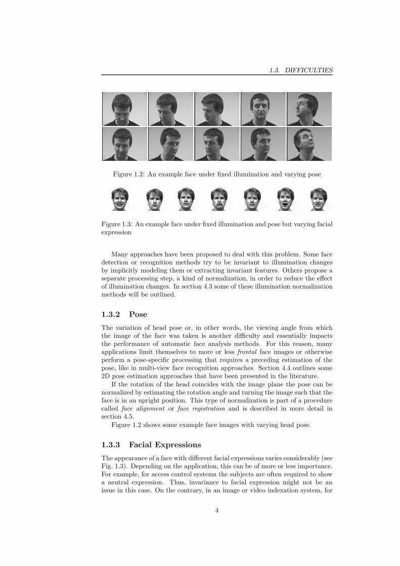
Figure 1.2: An example face under fixed illumination and varying pose
Figure 1.3: An example face under fixed illumination and pose but varying facialexpression
Many approaches have been proposed to deal with this problem. Some facedetection or recognition methods try to be invariant to illumination changesby implicitly modeling them or extracting invariant features. Others propose aseparate processing step, a kind of normalization, in order to reduce the effectof illumination changes. In section 4.3 some of these illumination normalizationmethods will be outlined.
1.3.2 Pose
The variation of head pose or, in other words, the viewing angle from whichthe image of the face was taken is another difficulty and essentially impactsthe performance of automatic face analysis methods. For this reason, manyapplications limit themselves to more or less frontal face images or otherwiseperform a pose-specific processing that requires a preceding estimation of thepose, like in multi-view face recognition approaches. Section 4.4 outlines some2D pose estimation approaches that have been presented in the literature.
If the rotation of the head coincides with the image plane the pose can benormalized by estimating the rotation angle and turning the image such that theface is in an upright position. This type of normalization is part of a procedurecalled face alignment or face registration and is described in more detail insection 4.5.
Figure 1.2 shows some example face images with varying head pose.
1.3.3 Facial Expressions
The appearance of a face with different facial expressions varies considerably (seeFig. 1.3). Depending on the application, this can be of more or less importance.For example, for access control systems the subjects are often required to showa neutral expression. Thus, invariance to facial expression might not be anissue in this case. On the contrary, in an image or video indexation system, for
4

CHAPTER 1. INTRODUCTION
example, this would be more important as the persons are shown in every-daysituations and might speak, smile, laugh etc.
In general, the mouth is subject to the largest variation. The respectiveperson on an image can have an open or closed mouth, can be speaking, smiling,laughing or even making grimaces.
Eyes and eyebrows are also changing subject to varying facial expressions,e.g. when the respective person blinks, sleeps or widely opens his/her eyes.
1.3.4 Partial Occlusions
Partial occlusions occur quite frequently in real-world face images. They canbe caused by a hand occluding a part of the face, e.g. the mouth, by long hear,glasses, sun glasses or other objects or persons.
In most of the cases, however, the face occludes parts of itself. For example,in a view from the side the other side of the face is hidden. Also, a part ofthe cheek can be occluded by the nose or an eye can be covered by its orbit forexample.
1.3.5 Other types of variations
Appearance variations a also caused by varying make-up, varying hair-cut andthe presence of facial hear (beard, mustache etc.).
Varying age is also an important factor influencing the performance of manyface analysis methods. This is the case for example in face recognition when thereference face image has been taken some years before the image to recognize.
Finally, there are also variations across the subjects’ identities, such as race,skin color or, more generally, ethnic origin. The respective differences in theappearance of the face images can cause difficulties in applications like face orfacial feature detection or gender recognition.
1.4 Objectives
The goals pursued in this work principally concern the evaluation of Convo-lutional Neural Networks (CNN) in the context of facial analysis applications.More specifically, we will focus on the following objectives:
• evaluate the performance of CNNs w.r.t. appearance-based facial analysis
• investigate the robustness of CNNs against classical sources of noise in thecontext of facial analysis
• propose different CNN architectures designed for specific facial analysisproblems such as face alignment, facial feature detection, face recognitionand gender classification
• improve upon the state-of-the-art in appearance-based facial feature detec-tion, face alignment as well as face recognition under real-world conditions
• investigate different solutions improving the performance of automatic facerecognition systems
5
1.5. OUTLINE
1.5 Outline
In the following chapter we will outline some of the most important machinelearning techniques used for object detection and recognition in images, suchas statistical projection methods, Hidden Markov Models, Support Vector Ma-chines and Neural Networks.
In chapter 3, we will then focus on one particular approach, called Con-volutional Neural Networks (CNN), which is the foundation for the methodsproposed in this work.
Having described, among other aspects, the principle architecture and train-ing methods for CNNs, in chapter 4 we will outline the problem of face detectionand normalization and how CNNs can tackle these types of problems. Usingan existing CNN-based face detection system, called Convolutional Face Finder(CFF), we will further present an effective approach for face alignment whichis an important step in many facial analysis applications.
In chapter 5, we will describe the problem of facial feature detection whichshows to be crucial for any facial image processing task. We will propose an ap-proach based on a specific type of CNN to solve this problem and experimentallyshow its performance in terms of precision and robustness to noise.
Chapter 6 outlines two further facial analysis problems, namely automaticface recognition and gender recognition. We will also present CNN-based ap-proaches to these problems and experimentally show their effectiveness com-pared to other machine learning techniques proposed in the literature.
Finally, chapter 7 will conclude this work with a short summary and someperspectives for future research.
6

Chapter 2
Machine Learning
Techniques for Object
Detection and Recognition
2.1 Introduction
In this chapter we will outline some of the most common machine learningapproaches to object detection and recognition. Machine Learning techniquesautomatically learn from a set of examples how to classify new instances ofthe same type of data. The capacity to generalize, i.e. the ability to success-fully classify unknown data and possibly infer generic rules or functions, is animportant property of these approaches and is sought to be maximized.
Usually, one distinguishes between three types of learning:
Supervised learning A training set and the corresponding desired outputs ofthe function to learn are available. Thus, during training the algorithmiteratively presents examples to the system and adapts its parametersaccording to the distance between the produced and the desired outputs.
Unsupervised learning The underlying structure of the training data, i.e.the desired output, is unknown and is to be determined by the trainingalgorithm. For example, for a classification method this means that theclass information is not available and has to be approximated by groupingthe training examples using some distance measure, a technique calledclustering.
Reinforcement learning Here, the exact output of the function to learn isunknown, and training consists in a parameter adjustment based on onlytwo concepts, reward and penalty. That is, if the system does not performwell (enough) it is “penalized” and the parameters are adapted accord-ingly. Otherwise, it is “rewarded”, i.e. some positive reinforcement takesplace.
Most of the algorithms described in the following are supervised, but theyare employed for rather different purposes: some of them are used to extract
7
2.2. STATISTICAL PROJECTION METHODS
features from the input data, some are used to classify the extracted features,and others perform both tasks.
The application context varies also largely, i.e. some of the approaches canbe used for detection of features and/or objects, some only for recognition andothers for both. Further, in many systems a combination of several of thetechniques described in this chapter is used. Thus, in a sense, they could beconsidered as some kind of building blocks for effective object detection andrecognition systems.
Let us begin with some of the most universal techniques used in machinelearning which are based on a statistical analysis of the data allowing to signif-icantly reduce its dimensionality and extract valuable information.
2.2 Statistical Projection Methods
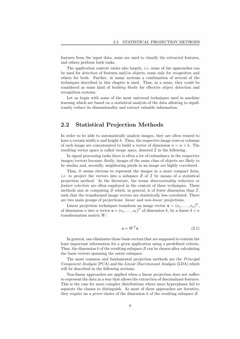
In order to be able to automatically analyze images, they are often resized tohave a certain width w and height h. Then, the respective image rows or columnsof each image are concatenated to build a vector of dimension n = w × h. Theresulting vector space is called image space, denoted I in the following.
In signal processing tasks there is often a lot of redundancy in the respectiveimages/vectors because, firstly, images of the same class of objects are likely tobe similar and, secondly, neighboring pixels in an image are highly correlated.
Thus, it seems obvious to represent the images in a more compact form,i.e. to project the vectors into a subspace S of I by means of a statisticalprojection method. In the literature, the terms dimensionality reduction orfeature selection are often employed in the context of these techniques. Thesemethods aim at computing S which, in general, is of lower dimension than I,such that the transformed image vectors are statistically less correlated. Thereare two main groups of projections: linear and non-linear projections.
Linear projection techniques transform an image vector x = (x1, . . . , xn)T ,of dimension n into a vector s = (s1, . . . , sk)T of dimension k, by a linear k× ntransformation matrix W :
s = WTx (2.1)
In general, one eliminates those basis vectors that are supposed to contain theleast important information for a given application using a predefined criteria.Thus, the dimension k of the resulting subspace S can be chosen after calculatingthe basis vectors spanning the entire subspace.
The most common and fundamental projection methods are the PrincipalComponent Analysis (PCA) and the Linear Discriminant Analysis (LDA) whichwill be described in the following sections.
Non-linear approaches are applied when a linear projection does not sufficeto represent the data in a way that allows the extraction of discriminant features.This is the case for more complex distributions where mere hyperplanes fail toseparate the classes to distinguish. As most of these approaches are iterative,they require an a priori choice of the dimension k of the resulting subspace S.
8
CHAPTER 2. MACHINE LEARNING TECHNIQUES FOR OBJECT
DETECTION AND RECOGNITION
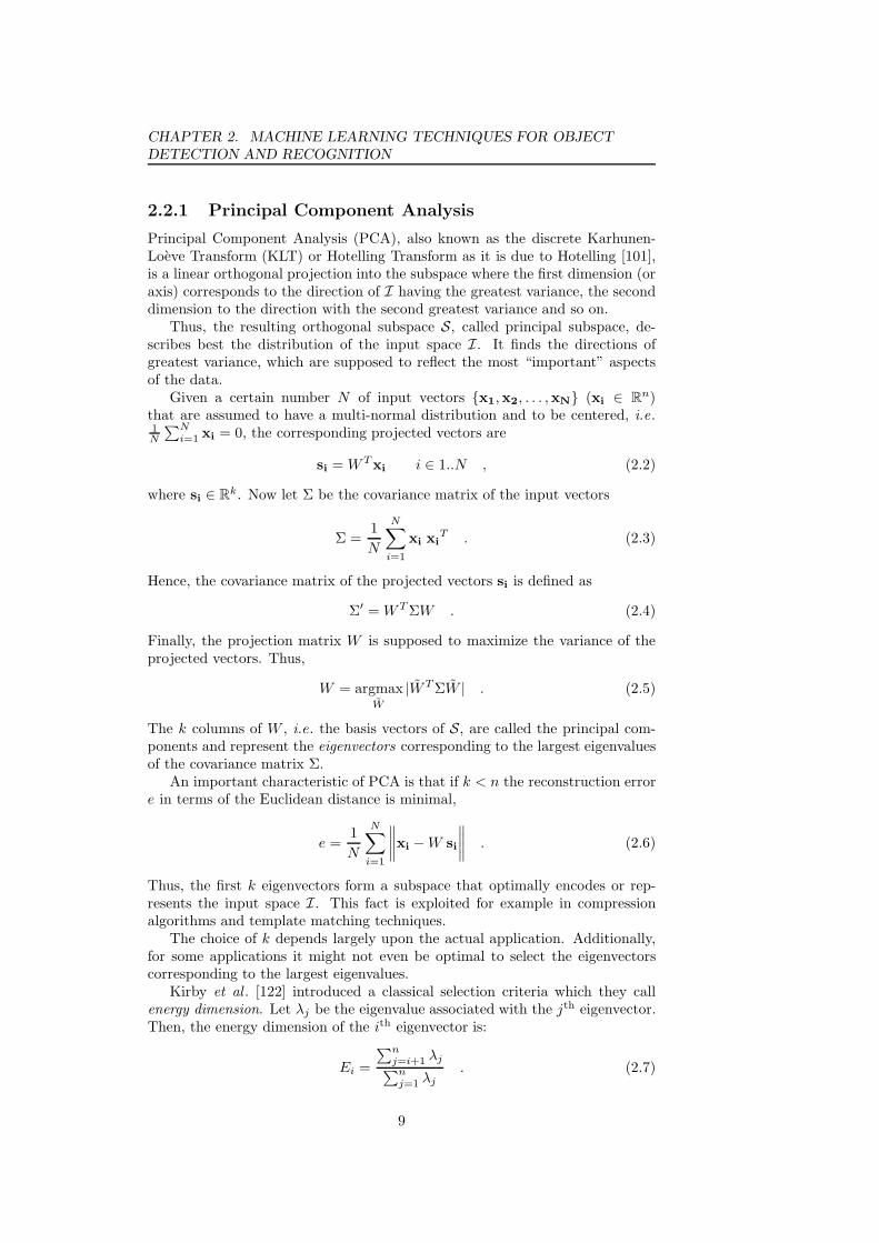
2.2.1 Principal Component Analysis
Principal Component Analysis (PCA), also known as the discrete Karhunen-Loeve Transform (KLT) or Hotelling Transform as it is due to Hotelling [101],is a linear orthogonal projection into the subspace where the first dimension (oraxis) corresponds to the direction of I having the greatest variance, the seconddimension to the direction with the second greatest variance and so on.
Thus, the resulting orthogonal subspace S, called principal subspace, de-scribes best the distribution of the input space I. It finds the directions ofgreatest variance, which are supposed to reflect the most “important” aspectsof the data.
Given a certain number N of input vectors x1,x2, . . . ,xN (xi ∈ Rn)
that are assumed to have a multi-normal distribution and to be centered, i.e.1N
∑Ni=1 xi = 0, the corresponding projected vectors are
si = WTxi i ∈ 1..N , (2.2)
where si ∈ Rk. Now let Σ be the covariance matrix of the input vectors
Σ =1
N
N∑
i=1
xi xiT . (2.3)
Hence, the covariance matrix of the projected vectors si is defined as
Σ′ = WT ΣW . (2.4)
Finally, the projection matrix W is supposed to maximize the variance of theprojected vectors. Thus,
W = argmaxW
|WT ΣW | . (2.5)
The k columns of W , i.e. the basis vectors of S, are called the principal com-ponents and represent the eigenvectors corresponding to the largest eigenvaluesof the covariance matrix Σ.
An important characteristic of PCA is that if k < n the reconstruction errore in terms of the Euclidean distance is minimal,
e =1
N
N∑
i=1
∥∥∥∥xi −W si
∥∥∥∥
. (2.6)
Thus, the first k eigenvectors form a subspace that optimally encodes or rep-resents the input space I. This fact is exploited for example in compressionalgorithms and template matching techniques.
The choice of k depends largely upon the actual application. Additionally,for some applications it might not even be optimal to select the eigenvectorscorresponding to the largest eigenvalues.
Kirby et al . [122] introduced a classical selection criteria which they callenergy dimension. Let λj be the eigenvalue associated with the jth eigenvector.Then, the energy dimension of the ith eigenvector is:
Ei =
∑nj=i+1 λj∑n
j=1 λj
. (2.7)
9

2.2. STATISTICAL PROJECTION METHODS
One can show that the Mean Squared Error (MSE) produced by the last n−i re-jected eigenvectors is
∑nj=i+1 λj . The selection of k now consists in determining
a threshold τ such that Ek−1 > τ and Ek < τ .Apart from image compression and template matching, PCA is often applied
to classification tasks, e.g. the Eigenfaces approach [243] in face recognition.Here, the projected vectors si are the signatures to be classified. To this end,the signatures of the N input images are each associated with a class label andused to build a classifier. The most simple classifier would be a nearest neighborclassifier using an Euclidean distance measure.
To sum up, PCA calculates the linear orthogonal subspace having its axesoriented with the directions of greatest variances. It thus optimally representsthe input data. However, in a classification context it is not guaranteed thatin the subspace calculated by PCA the separability of the data is improved. Inthis regard, the Linear Discriminant Analysis (LDA) described in the followingsection is more suitable.
2.2.2 Linear Discriminant Analysis
The Linear Discriminant Analysis (LDA) has been introduced by Fisher [69]in 1936 but generalized later on to the so-called Fisher’s Linear Discriminant(FLD). It is, in contrast to the PCA, not only concerned with the best repre-sentation of the data but also with its separability in the projected subspacewith regard to the different classes.
Let Ω = x1, . . .xN be the training set partitioned into c annotated classesdenoted Ωi (i ∈ 1..c). We are now searching the subspace S that maximizes theinter-class variability while minimizing the intra-class variability, thus improvingthe separability of the respective classes. To this end, one maximizes the so-called Fisher’s criterion [69, 16]:
J(W ) =|WT ΣbW |
|WT ΣwW |. (2.8)
Thus,
W = argmaxW
|WT ΣbW |
|WT ΣwW |, (2.9)
where
Σw =1
N
c∑
j=1
∑
xi∈Ωj
(xi − xj)(xi − xj)T (2.10)
represents the within-class variance and
Σb =1
N
c∑
j=1
Nj(xj − x)(xj − x)T (2.11)
the between-class variance. Nj is the number of examples in Ωj (i.e. of class j)and xj are the respective means, i.e. xj = 1
Nj
∑
xi∈Ωjxi. x is the overall mean
of the data which is assumed to be centered, i.e. x = 0.The projection matrix W is obtained by calculating the eigenvectors associ-
ated with the largest eigenvalues of the matrix Σ−1w Σb. These eigenvectors form
the columns of W .
10

CHAPTER 2. MACHINE LEARNING TECHNIQUES FOR OBJECT
DETECTION AND RECOGNITION
A problem occurs when the number of examples N is smaller than the size ofthe input vectors, i.e. for images the number of pixels n. Then, Σw is singularsince its rank is at most N−c. The calculation of Σ−1
w is thus impossible. Severalapproaches have been proposed to overcome this problem. One is to produceadditional examples by adding noise to the images of the training database.Another approach consists in first applying PCA to reduce the input vectorspace to the dimension N − c and then perform LDA as described above.
2.2.3 Other Projection Methods
There are many other projection techniques proposed in the literature and whichcan possibly be applied to object detection and recognition.
For example, Independent Component Analysis (ICA) [17, 2, 35, 109, 108] isa technique often used for blind source separation [120], i.e. to find the differentindependent sources a given signal is composed of. ICA seeks a linear sub-spacewhere the data is not only uncorrelated but statistically independent. In itsmost simple form, the model is the following:
x = AT s , (2.12)
where x is the observed data, s are the independent sources and A is the so-called mixing matrix. ICA consists in optimizing an objective function, denotedcontrast function, that can be based on different criteria. The contrast functionhas to ensure that the projected data is independent and non-Gaussian. Notethat ICA does not reduce the dimensionality of the input data. Hence, it isoften employed in combination with PCA or any other dimensionality reductiontechnique. Numerous implementations of ICA exist, e.g. INFOMAX [17], JADE[35] or FastICA [109].
Yang et al . [263] introduced the so-called two-dimensional PCA, which doesnot require the input image to be transformed into a one-dimensional vectorbeforehand. Instead, a generalized covariance matrix is directly estimated usingthe image matrices. Then, the eigenvectors are determined in a similar mannerthan for 1D-PCA by minimizing a special criterion based on this covariancematrix. Finally, in order to perform classification a distance measure betweenmatrix signatures has to be defined. It has been shown that this method outper-forms one-dimensional PCA in terms of classification rate [263] and robustness[254].
Visani et al . [252] presented a similar approach based on LDA: the two-dimensional oriented LDA. The procedure is analogical to the 2D-PCA methodwhere the projection is directly performed on the image matrices, either column-wise or row-wise. A generalized Fisher’s criterion is defined and minimized inorder to obtain the projection matrix. Further, the authors showed that incontrast to LDA, the two-dimensional oriented LDA can implicitly circumventthe singularity problem. In a later work [253], they generalized this approachto the Bilinear Discriminant Analysis (BDA) where column-wise and row-wise2D-LDA is iteratively applied to estimate the pair of projection matrices min-imizing an expression similar to the Fisher’s criterion which combines the twoprojections.
Note that the projection methods presented so far are all linear projectiontechniques. However, in some cases the different classes cannot be correctly
11

2.3. ACTIVE APPEARANCE MODELS
separated in a linear sub-space. Then, non-linear projection methods can helpto improve the classification rate. Most of the linear projection methods can bemade non-linear by projecting the input data into a higher-dimensional spacewhere the classes are more likely to be linearly separable. That means, theseparating hyperplane in this sub-space represents a non-linear sub-space of theinput vector space. Fortunately, it is not necessary to explicitly describe thishigher-dimensional space and the respective projection function if we find a so-called kernel function that implements a simple dot-product in this vector spaceand satisfies the Mercer’s condition (see Theorem 1 on p. 22). For a more formalexplanation see section 2.6.3 on non-linear SVMs. The kernel function allows toperform a dot-product in the target vector space and can be used to constructnon-linear versions of the previously described projection techniques e.g. PCA[219, 264], LDA [161] or ICA [6].
The projection approaches that have been outlined in this section can inprincipal be applied to any type of data in order to perform a statistical anal-ysis on the respective examples. A technique called Active Appearance Model(AAM) [41] can also be classified as a statistical projection approach but it ismuch more specialized to model images of deformable objects under varyingexternal conditions. Thus, in contrast to methods like PCA or LDA, where theinput image is treated as a “static” vector, small local deformations are takeninto account. AAMs have been especially applied to face analysis, and we willtherefore describe this technique in more detail in the following section.
2.3 Active Appearance Models
Active Appearance Models (AAM), introduced by Cootes et al . [41] as an exten-sion to Active Shape Models (ASM) [43], represent an approach that statisticallydescribes not only the texture of an object but also its shape. Given a new im-age of the class of objects to analyze, the idea is here to interpret the object bysynthesizing an image of the respective object while approximating as good aspossible its appearance in the real image. It has mainly been applied to faceanalysis problems [60, 41]. Therefore, face images we will used in the followingto illustrated this technique. Modeling the shape of faces appears to be helpfulin most face analysis applications where the face images are subject to changesin pose and facial expressions.
2.3.1 Modeling shape and appearance
The basis of the algorithm is a set of training images with a certain number of an-notated feature points, so-called landmark points, i.e. two-dimensional vectors.Each set of landmarks is represented as a single vector x, and PCA is appliedto the whole set of vectors. Thus any shape example can be approximated bythe equation:
x = x + Psbs , (2.13)
where x is the mean shape, and Ps is the linear subspace representing thepossible variations of shape parameterized by the vector bs.
Then, the annotated control points of each training example are matchedto the mean shape while warping the pixel intensities using a triangulationalgorithm. This leads to a so-called shape-free face patch for each example.
12

CHAPTER 2. MACHINE LEARNING TECHNIQUES FOR OBJECT
DETECTION AND RECOGNITION
Labelled image Points Shape−free patch
Figure 2.1: Active Appearance Models: annotated training example and corre-sponding shape-free patch
Figure 2.1 illustrates this with an example face image. Subsequently, a PCA isperformed on the gray values g of the shape-free images forming a statisticalmodel of texture:
g = g + Pgbg , (2.14)
where g represents the mean texture, and the matrix Pg linearly describes thetexture variations parameterized by the vector bg.
Since shape and texture are correlated, another PCA is applied on the con-catenated vectors of bs and bg leading to the combined model:
x = x + Qsc (2.15)
g = g + Qgc , (2.16)
where c is a parameter controlling the overall appearance, i.e. both shape andtexture, and Qs and Qg represent the combined linear shape-texture subspace.
Given a parameter vector c, the respective face can be synthesized by firstbuilding the shape-free image, i.e. the texture, using equation 2.16 and thenwarping the face image by applying equation 2.15 and the triangulation algo-rithm used to build the shape-free patches.
2.3.2 Matching the model
Having built the statistical shape and texture models, the objective is to matchthe model to an image by synthesizing the approximate appearance of the objectin the real image. Thus, we want to minimize:
∆ = |Ii − Im| , (2.17)
where Ii is the vector of gray-values of the real image and Im is the one of thesynthesized image.
The approach assumes that the object is roughly localized in the input image,i.e. during the matching process, the model with its landmark points must notbe too far away from the resulting locations.
Now, the decisive question is how to change the model parameters c in orderto minimize ∆. A good approximation appears to be a linear model:
δc = A(Ii − Im) , (2.18)
13

2.4. HIDDEN MARKOV MODELS
where A is determined by a multi-variate linear regression on the training dataaugmented by examples with manually added perturbations.
To calculate Ii − Im, the respective real and synthesized images are trans-formed to be shape-free using a preliminary estimate of the shape model. Thus,we compute:
δg = gi − gm (2.19)
and obtainδc = Aδg . (2.20)
This linear approximation shows to perform well over a limited range of themodel parameters, i.e. about 0.5 standard deviations of the training data.
Finally, this estimation is put into an iterative framework, i.e. at each iter-ation we calculate:
c′ = c−Aδg (2.21)
until convergence, where the matrix A is scaled such that it minimizes |δg|.The final result can then be used, for example, to localize specific feature
points, to estimate the 3D orientation of the object, to generate a compressedrepresentation of the image or, in the context of face analysis, to identify therespective person, gender or facial expression.
Clearly, AAMs can cope with small local image transformations and ele-gantly model shape and texture of an object based on a preceding statisticalanalysis of the training examples. However, the resulting projection space canbe rather large, and the search in this space, i.e. the matching process, can beslow. A fundamentally different approach to take into account local transfor-mations of a signal are Hidden Markov Models (HMM). This is a probabilisticmethod that represents a signal, e.g. an image, as a sequence of observations.The following section outlines this approach.
2.4 Hidden Markov Models
2.4.1 Introduction
Hidden Markov Models (HMM), introduced by Rabiner et al . [190, 191], arecommonly used to model the sequential aspect of data. In the signal process-ing context for example, they have been frequently applied to speech recog-nition problems modeling the temporal sequence of states and observations,e.g. phonemes. An image can also be seen as a sequence of observations, e.g.image subregions, and here the image either has to be linearized into a one-dimensional structure or special types of HMMs have to be used, for exampletwo-dimensional Pseudo HMMs or Markov Random Fields.
Being the most common approaches in image analysis, we will focus on 1Dand Pseudo 2D HMMs in the following. The major disadvantage of “real” 2DHMMs is their relatively high complexity in terms of computation time.
A HMM is characterized by a finite number of states, and it can be in onlyone state at a time (as a finite state machine). The initial state probabilitiesdefine, for every state, the probability of the HMM being in that state at timet = 1. For each following time step t = 2..T it can either change the state or stayin the same state with a certain probability defined by the so-called transitionprobabilities. Further, in any state it creates an output from a pre-defined
14

CHAPTER 2. MACHINE LEARNING TECHNIQUES FOR OBJECT
DETECTION AND RECOGNITION
State 3State 2State 1
Figure 2.2: A left-right Hidden Markov Model
vocabulary with a certain probability, determined by the output probabilities.At time t = T the HMM will have produced a certain sequence of outputs,called observations; O = o1, . . . , oT . The sequence of states Q = q1, . . . , qT it has traversed, however, is unknown (hidden) and has to be estimated byanalyzing the observation whereas a single observation could be produced bydifferent state sequences.
Fig. 2.2 illustrates a simple example of a HMM with 3 states. This type ofHMM is called left-right model or Bakis model.
More formally we can describe a HMM as follows:
Definition 1 A Hidden Markov Model is defined as λ = S, V, A, B, Π, where
• S = s1, . . . , sN is the set of N possible states,
• V = v1, . . . , vL is the set of L possible outputs constituting the vocabu-lary,
• A = aiji,j=1..N is the set transition probabilities from state i to state j,
• B = bi(l)i=1..N,l=1..L define the output probabilities of output l in statei,
• Π = π1, . . . , πN is the set of initial state probabilities.
Note thatN∑
i=1
πi = 1 , (2.22)
N∑
j=1
aij = 1 ∀i = 1, . . . , N and (2.23)
L∑
l=1
bi(l) = 1 ∀i = 1, . . . , N . (2.24)
Given a HMM λ, the goal is to determine the probability of a new observationsequence O = o1, . . . , oT , i.e. P [O|λ]. For this purpose, there are severalalgorithms, the most simple one being explained in the following section.
2.4.2 Finding the most likely state sequence
There are many algorithms for estimating P [O|λ] and the most likely statesequence Q∗ = q∗1 , . . . , q
∗T having generated O. The most well known of these
are called Viterbi algorithm and Baum-Welsh algorithm. Algorithm 1 describesthe former which is a kind of simplification of the latter. Note that δti denotes
15

2.4. HIDDEN MARKOV MODELS
Algorithm 1 The Viterbi algorithm
for i = 1 to N do
δ1i = πibi(o1)end for
for t = 2 to T do
for i = 1 to N do
δti = bi(ot)maxδt−1,jaji ∀j = 1..Nφti = sj where j = argmaxjδt−1,jaji ∀j = 1..N
end for
end for
P [O|λ] = maxδTj ∀j = 1..Nq∗T = argmaxjδTj ∀j = 1..Nfor t = T − 1 to 1 do
q∗t = φt+1,q∗
t+1
end for
the probability of being in state si at time t, and φti denotes the most probablepreceding state being in si at time t. Thus, the φti store the most probable statesequence. The last loop allows to retrieve the final most likely state sequenceQ∗ by recursively traversing φti.
When applying a HMM to a given observation sequence O it suffices for mostapplications to calculate P [O|λ] as stated above. The actual state sequence Q∗
however is necessary for the training process explained in the following section.
2.4.3 Training
In order to automatically determine and re-adjust the parameters of λ a set oftraining observations Otr = ot1, . . . , otM is used, and a training algorithm,for example algorithm 1, is applied to estimate the probabilities: P [Otr|λ] andP [Otr, qt = si|λ] for every state si at every time step t.
Then each parameter can be re-estimated by re-generating the observationsequences Otr and “counting” the number of events determining the respectiveparameter. For example, to adjust aij one calculates:
a′ij =
expected number of transitions from si to sj
expected number of transitions from si
=P [qt = si, qt+1 = sj |Otr , λ]
P [qt = si|Otr , λ](2.25)
The output probabilities B and the initial state probabilities Π are estimatedin an analogical way. However, the number and topology of states S has to bedetermined experimentally in most cases.
2.4.4 HMMs for Image Analysis
HMMs are one-dimensional models and have initially been applied to the pro-cessing of audio data [190]. However, there are several approaches to adapt thistechnique to 2D data like images.
16
CHAPTER 2. MACHINE LEARNING TECHNIQUES FOR OBJECT
DETECTION AND RECOGNITION
...
(a) 1D HMM based on image bands
...
(b) 1D HMM based on image blocks
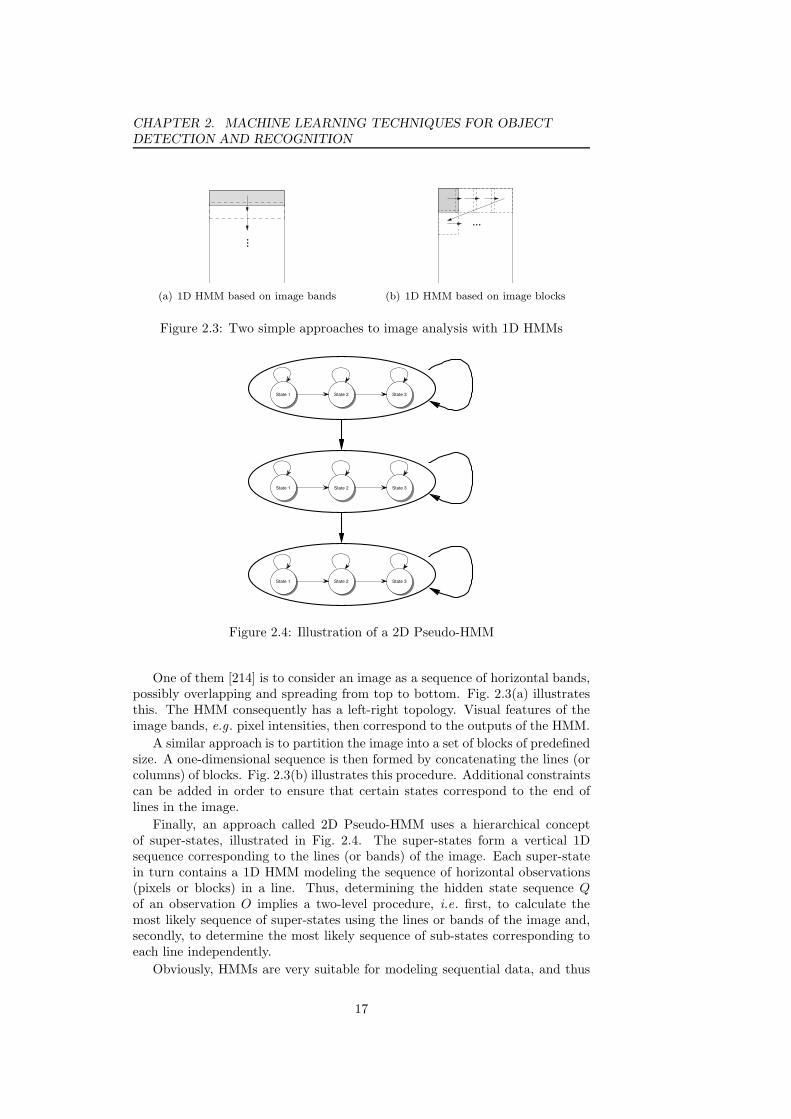
Figure 2.3: Two simple approaches to image analysis with 1D HMMs
State 3State 2State 1
State 3State 2State 1
State 3State 2State 1
Figure 2.4: Illustration of a 2D Pseudo-HMM
One of them [214] is to consider an image as a sequence of horizontal bands,possibly overlapping and spreading from top to bottom. Fig. 2.3(a) illustratesthis. The HMM consequently has a left-right topology. Visual features of theimage bands, e.g. pixel intensities, then correspond to the outputs of the HMM.
A similar approach is to partition the image into a set of blocks of predefinedsize. A one-dimensional sequence is then formed by concatenating the lines (orcolumns) of blocks. Fig. 2.3(b) illustrates this procedure. Additional constraintscan be added in order to ensure that certain states correspond to the end oflines in the image.
Finally, an approach called 2D Pseudo-HMM uses a hierarchical conceptof super-states, illustrated in Fig. 2.4. The super-states form a vertical 1Dsequence corresponding to the lines (or bands) of the image. Each super-statein turn contains a 1D HMM modeling the sequence of horizontal observations(pixels or blocks) in a line. Thus, determining the hidden state sequence Qof an observation O implies a two-level procedure, i.e. first, to calculate themost likely sequence of super-states using the lines or bands of the image and,secondly, to determine the most likely sequence of sub-states corresponding toeach line independently.
Obviously, HMMs are very suitable for modeling sequential data, and thus
17
2.5. ADABOOST
they are principally used in signal processing tasks. Let us now consider somemore general machine learning techniques which do not explicitely model thissequential aspect but, on the other hand, can more easily and efficiently beapplied to higher dimensional data such as images. Adaptive Boosting is onesuch approach and will be explained in the following section.
2.5 Adaboost
2.5.1 Introduction
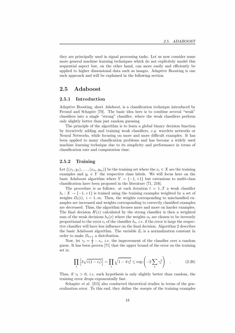
Adaptive Boosting, short Adaboost, is a classification technique introduced byFreund and Schapire [70]. The basic idea here is to combine several “weak”classifiers into a single “strong” classifier, where the weak classifiers performonly slightly better than just random guessing.
The principle of the algorithm is to learn a global binary decision functionby iteratively adding and training weak classifiers, e.g. wavelets networks orNeural Networks, while focusing on more and more difficult examples. It hasbeen applied to many classification problems and has become a widely usedmachine learning technique due to its simplicity and performance in terms ofclassification rate and computation time.
2.5.2 Training
Let (x1, y1), . . . , (xm, ym) be the training set where the xi ∈ X are the trainingexamples and yi ∈ Y the respective class labels. We will focus here on thebasic Adaboost algorithm where Y = −1, +1 but extensions to multi-classclassification have been proposed in the literature [71, 216].
The procedure is as follows: at each iteration t = 1..T a weak classifierht : X → −1, +1 is trained using the training examples weighted by a set ofweights Dt(i), i = 1..m. Then, the weights corresponding to misclassified ex-amples are increased and weights corresponding to correctly classified examplesare decreased. Thus, the algorithm focuses more and more on harder examples.The final decision H(x) calculated by the strong classifier is then a weightedsum of the weak decisions ht(x) where the weights αt are chosen to be inverselyproportional to the error ǫt of the classifier ht, i.e. if the error is large the respec-tive classifier will have less influence on the final decision. Algorithm 2 describesthe basic Adaboost algorithm. The variable Zt is a normalization constant inorder to make Dt+1 a distribution.
Now, let γt = 12 − ǫt, i.e. the improvement of the classifier over a random
guess. It has been proven [71] that the upper bound of the error on the trainingset is:
∏
t
[
2√
ǫ(1− ǫt)]
=∏
t
√
1− 4γ2t ≤ exp
(
−2∑
t
γ2t
)
. (2.26)
Thus, if γt > 0, i.e. each hypothesis is only slightly better than random, thetraining error drops exponentially fast.
Schapire et al . [215] also conducted theoretical studies in terms of the gen-eralization error. To this end, they define the margin of the training examples
18
CHAPTER 2. MACHINE LEARNING TECHNIQUES FOR OBJECT
DETECTION AND RECOGNITION
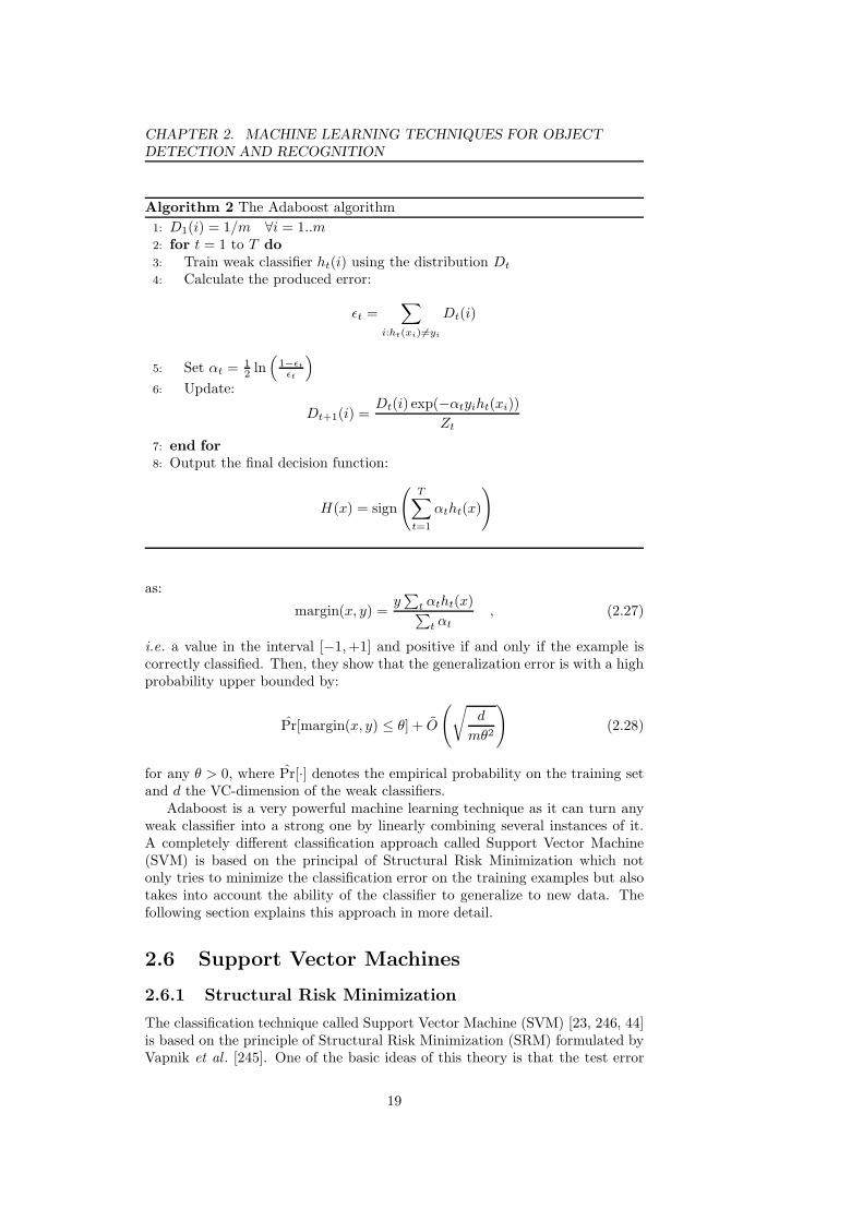
Algorithm 2 The Adaboost algorithm
1: D1(i) = 1/m ∀i = 1..m2: for t = 1 to T do
3: Train weak classifier ht(i) using the distribution Dt
4: Calculate the produced error:
ǫt =∑
i:ht(xi) 6=yi
Dt(i)
5: Set αt = 12 ln
(1−ǫt
ǫt
)
6: Update:
Dt+1(i) =Dt(i) exp(−αtyiht(xi))
Zt
7: end for
8: Output the final decision function:
H(x) = sign
(T∑
t=1
αtht(x)
)
as:
margin(x, y) =y∑
t αtht(x)∑
t αt
, (2.27)
i.e. a value in the interval [−1, +1] and positive if and only if the example iscorrectly classified. Then, they show that the generalization error is with a highprobability upper bounded by:
Pr[margin(x, y) ≤ θ] + O
(√
d
mθ2
)
(2.28)
for any θ > 0, where Pr[·] denotes the empirical probability on the training setand d the VC-dimension of the weak classifiers.
Adaboost is a very powerful machine learning technique as it can turn anyweak classifier into a strong one by linearly combining several instances of it.A completely different classification approach called Support Vector Machine(SVM) is based on the principal of Structural Risk Minimization which notonly tries to minimize the classification error on the training examples but alsotakes into account the ability of the classifier to generalize to new data. Thefollowing section explains this approach in more detail.
2.6 Support Vector Machines
2.6.1 Structural Risk Minimization
The classification technique called Support Vector Machine (SVM) [23, 246, 44]is based on the principle of Structural Risk Minimization (SRM) formulated byVapnik et al . [245]. One of the basic ideas of this theory is that the test error
19

2.6. SUPPORT VECTOR MACHINES
rate, or structural risk R(α), is upper bounded by the training error rate, orempirical risk Remp and an additional term called VC-confidence which dependson the so-called Vapnik-Chervonenkis (VC)-dimension h of the classificationfunction. More precisely, with the probability 1− η, the following holds [246]:
R(α) ≤ Remp(α) +
√
h(log(2l/h) + 1)− log(η/4)
l, (2.29)
where α are the parameters of the function to learn and l is the number oftraining examples. The VC-dimension h of a class of functions describes its“capacity” to classify a set of training data points. For example, in the case ofa two-class classification problem, if a function f has a VC-dimension of h thereexists at least one set of h data points that can be correctly classified by f , i.e.assigned the label −1 or +1 to it. If the VC-dimension is too high the learningmachine will overfit and show poor generalization. If it is too low, the functionwill not sufficiently approximate the distribution of the data and the empiricalerror will be too high. Thus, the goal of SRM is to find a h that minimizes thestructural risk R(α), which is supposed to lead to maximum generalization.
2.6.2 Linear Support Vector Machines
Vapnik [246] showed that for linear hyperplane decision functions:
f(x) = sign((w · x) + b) (2.30)
the VC-dimension is determined by the norm of the weight vector w.Let (xi, yi), . . . , (xl, yl) (xi ∈ R
n, yi ∈ −1, +1) be the training set.Then, for a linearly separable training set we have:
yi(xi ·w + b)− 1 ≥ 0 ∀i = 1..l . (2.31)
The margin between the positive and negative points is defined by two hyper-planes x ·w + b = ±1 where the above term actually is zero. Fig. 2.5 illustratesthis. Further, no points lie between these hyperplanes and the width of the mar-gin is 2/||w||. The support vector algorithm now tries to maximize the marginby minimizing ||w||, which is supposed to be an optimal solution, i.e. wheregeneralization is maximal. Once the maximum margin is obtained, data pointslying on one of the separating hyperplanes, i.e. for which equation 2.31 yieldszero, are called support vectors (illustrated by double circles in Fig. 2.5).
To simplify the calculation, the problem is formulated in a Lagrangian frame-work (see [246] for details). This leads to the maximization of the Lagrangians:
LD =
l∑
i=1
αi −1
2
∑
ij
αiαjyiyj xi · xj (2.32)
subject to
w =
l∑
i=1
αiyixi , (2.33)
l∑
i=1
αiyi = 0 and (2.34)
20

CHAPTER 2. MACHINE LEARNING TECHNIQUES FOR OBJECT
DETECTION AND RECOGNITION
margin
w
w · x + b > 0w · x + b < 0
Figure 2.5: Graphical illustration of a linear SVM
αi ≥ 0 ∀i = 1..l , (2.35)
where αi (i = 1..l) are the Lagrangian multipliers that are to be determined.Further, the solutions to αi and condition 2.31 imply a value for b. Note thatall αi are zero except those corresponding to the support vectors.
Finally, new examples can simply be classified using the decision function2.30.
In many cases, however, the training data cannot be completely separatedbecause of some “outliers”. Then, we might simply loosen the constraint 2.31by introducing the constants ξi > 0 in the following way:
yi(xi ·w + b) ≥ (1− ξi) ∀i = 1..l , (2.36)
and condition 2.35 becomes
0 ≤ αi ≤ ξi ∀i = 1..l . (2.37)
2.6.3 Non-linear Support Vector Machines
In order to use a non-linear decision function, the above formulas can quiteeasily be generalized. Boser et al . [23] proposed a simple method based on theso-called kernel trick. That is, before applying the dot product xi ·xj in equation2.32 the d-dimensional data is projected into a higher dimensional space whereit is supposed to be linearly separable. Thus, a function Φ : R
d → H is definedand xi · xj becomes Φ(xi) · Φ(xj). Now, instead of calculating Φ each time weuse a kernel function K(xi,xj) = Φ(xi) · Φ(xj), i.e. each occurrence of the dotproduct is replaced by K(·, ·). Thus, if we want to classify a new data point s
the decision function
f(x) = sign
(l∑
i=1
αiyi xi · s + b
)
(2.38)
21
2.7. BAG OF LOCAL SIGNATURES
becomes
f(x) = sign
(l∑
i=1
αiyi Φ(xi) ·Φ(s) + b
)
= sign
(l∑
i=1
αiyi K(xi, s) + b
)
.
(2.39)With the kernel function K we don’t need to calculate Φ or H but we must
know if for a given K there exists a mapping Φ and some space H in which Kis the dot product K(xi,xj) = Φ(xi) · Φ(xj). This property is ensured by theMercer’s condition [246]:
Theorem 1 There exists a mapping Φ and an expansion
K(x,y) =∑
k
Φ(x)kΦ(y)k (2.40)
if and only if, for any g(x) such that
∫
g(x)2 dx is finite (2.41)
then ∫
K(x,y)g(x)g(y) dxdy ≥ 0 . (2.42)
Some examples for which the condition is satisfied are:
K(x,y) = (x · y + 1)n polynomial kernels (2.43)
K(x,y) = e−γ||x−y||2 Gaussian radial basis function (RBF) kernels(2.44)
K(x,y) = tanh(κ(x · y)− δ) sigmoid kernels (2.45)
2.6.4 Extension to multiple classes
Up to this point, we only considered two-class problems. However, there aresimple ways to extend the SVM method to several classes. One approach, calledone-against-all, consists in training one classifier for each class that distinguishesbetween the examples of that class and the examples of all other classes. Thus,the number of SVMs equals the number of classes n.
Another approach trains a SVM for each possible pair of classes. To classifyan example, it is input to each SVM and the class label corresponding to themaximal number of “winning” SVMs represents the final answer. The numberof classifiers needed by this approach is n(n−1)/2, which is a drawback in termsof complexity compared to the first approach.
2.7 Bag of Local Signatures
As opposed to SVMs, being a very general classification technique, an approachcalled Bag-of-Local-Signatures (BOLS) has recently been introduced by Csurkaet al . [51] for image classification problems, particularly object detection and
22

CHAPTER 2. MACHINE LEARNING TECHNIQUES FOR OBJECT
DETECTION AND RECOGNITION
... ...
b) c) d) e)a)
s1
s2
s3
v1
v2
v3
di
Figure 2.6: The histogram creation procedure with the Bag-of-local-signatureapproach: a) input image I, b) detected salient points, c) extracted local signa-tures, d) quantized vectors (dictionary entries), e) histogram h(I).
recognition. It was motivated by the bag-of-words approach for text categoriza-tion which simply counts the number of pre-defined key words in a documentin order to classify it into one of several categories.
In the first step of the BOLS method, n salient points pi = (xi, yi) of theinput image are detected using an interest point detection algorithm, e.g. theHarris affine detector [162]. The small image region around each detected pointis then represented by some local descriptors, such as the Scale-Invariant FeatureTransform (SIFT) descriptors [148], leading to a local signature si for eachsalient point.
In the following step, the extracted signatures are classified applying anykind of vector quantization method. To this end, a dictionary of k representativesignatures dj (j = 1..k) is calculated from the training set using a clusteringalgorithm. For example, Csurka et al . [51] used the k-means clustering algorithmand Ros et al . [199] used a Self-Organizing Map (SOM).
Thus, for an image I to classify a bag of local signatures vi, i.e. entriesof the dictionary, is obtained representing the appearance of the object in theimage. However, for two different images of the same object the respectiverepresentations might differ due to the varying appearance in different views orpartial occlusions making an efficient comparison difficult.
Therefore, discrete histograms h(I) of the bag of local signatures vi are calcu-lated by simply counting the number of occurrences of the respective signatures.Finally, the histograms can be classified by using classical histogram distancemeasures, such as χ2 or the Earth Mover’s Distance (EMD) or by training aclassifier on the vectors obtained from the histogram values, such as a Bayesclassifier or SVMs [51].
Figure 2.6 illustrates the overall procedure for generating the Bag-of-Local-Signatures representation. A major advantage of this approach compared tostatistical projection methods, for example, is its robustness to partial occlusionsand to changing pose of the object to recognize. This is due to the purelylocal representation and the rotation- and scale-invariant description of the localimage patches.
As this technique is a relatively new approach in the field of machine learningand very specific to image classification we won’t describe it here in more detail.We will rather concentrate on a very versatile and powerful machine learningtechnique constituting the basis for all of the face analysis approaches proposedin this work, namely Artificial Neural Networks.
23

2.8. NEURAL NETWORKS
...
Σ φ(V )V
b
1x1
x2
xn
w1
w2
wn
y
Figure 2.7: The Perceptron
2.8 Neural Networks
2.8.1 Introduction
Artificial Neural Networks (ANN), short Neural Networks (NN), denote a ma-chine learning technique that has been inspired by the human brain and itscapacity to perform complex tasks by means of inter-connected neurons per-forming each a very simple operation. Likewise, a NN is a trainable structureconsisting of a set of inter-connected units, each implementing a very simplefunction, and together eventually performing a complex classification functionor approximation task.
2.8.2 Perceptron
The most well known type of neural unit is called Perceptron and has beenintroduced by Rosenblatt [200]. Its basic structure is illustrated in Fig. 2.7. Ithas n inputs and one output where the output is a simple function of the sumof the input signals x weighted by w and an additional bias b. Thus,
y = φ(x ·w + b) . (2.46)
Often, the bias is put inside the weight vector w such that w0 = b and theinput vector x is extended correspondingly to have x0 = 1. Equation 2.46 thenbecomes:
y = φ(x ·w) . (2.47)
where φ is the Heavyside step function:
φ : R→ R
φ(x) =
1 if x ≥ 00 else.
(2.48)
The Perceptron thus implements a very simple two-class classifier where w
is the separating hyperplane such that w · x ≥ 0 for examples from one classand w · x < 0 for examples from the other.
In 1962, Rosenblatt introduced the perceptron convergence theorem [201],a supervised training algorithm capable of learning arbitrary two-class classi-fication problems. However, Minsky and Papert [163] pointed out that thereare very simple classification problems where the perceptron fails, namely whenthe two classes are not linearly separable like in the XOR-problem, where the
24
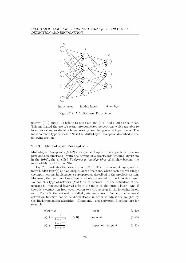
CHAPTER 2. MACHINE LEARNING TECHNIQUES FOR OBJECT
DETECTION AND RECOGNITION
input layer hidden layer output layer
x
y
z
Figure 2.8: A Multi-Layer Perceptron
pattern (0, 0) and (1, 1) belong to one class and (0, 1) and (1, 0) to the other.This motivated the use of several interconnected perceptrons which are able toform more complex decision boundaries by combining several hyperplanes. Themost common type of these NNs is the Multi-Layer Perceptron described in thefollowing section.
2.8.3 Multi-Layer Perceptron
Multi-Layer Perceptrons (MLP) are capable of approximating arbitrarily com-plex decision functions. With the advent of a practicable training algorithmin the 1980’s, the so-called Backpropagation algorithm [208], they became themost widely used form of NNs.
Fig. 2.8 illustrates the structure of a MLP. There is an input layer, one ormore hidden layer(s) and an output layer of neurons, where each neuron exceptthe input neurons implements a perceptron as described in the previous section.Moreover, the neurons of one layer are only connected to the following layer.We call this type of network: feed-forward network, i.e. the activation of theneurons is propagated layer-wise from the input to the output layer. And ifthere is a connection from each neuron to every neuron in the following layer,as in Fig. 2.8, the network is called fully connected. Further, the neurons’activation function has to be differentiable in order to adjust the weights bythe Backpropagation algorithm. Commonly used activation functions are forexample:
φ(x) = x linear (2.49)
φ(x) =1
1 + e−cx(c > 0) sigmoid (2.50)
φ(x) =1− e−x
1 + e−xhyperbolic tangent. (2.51)
25

2.8. NEURAL NETWORKS
-6
-4
-2
0
2
4
6
-4 -2 0 2 4
(a) linear
0
0.5
1
-4 -2 0 2 4
(b) sigmoid
-1
-0.5
0
0.5
1
-4 -2 0 2 4
(c) hyperbolic tangent
Figure 2.9: Different types of activation functions
input outputhidden“bottleneck”
(a) 3-layer AANN
input outputhidden 1 hidden 2 hidden 3
“bottleneck”
(b) 5-layer AANN
Figure 2.10: Auto-Associative Neural Networks
Figure 2.9 shows the three types of functions. Note that the linear function is inthe range ]−∞, +∞[, the sigmoid function in ]0, +1[ and the hyperbolic tangentfunction in ] − 1, +1[. The linear activation function is mostly bounded by amaximum and minimum value, e.g. −1 and +1, and thus it becomes a step-wiselinear function. However, when using the Backpropagation learning algorithm(explained in section 2.8.5) one has to be careful with the points where thestep-wise function is not differentiable, e.g. x = −1 and x = +1.
2.8.4 Auto-Associative Neural Networks
Auto-Associative Neural Networks (AANN) [47, 46, 86] are a special type ofMLP where the hidden layer has fewer neurons than the input and output layers,a so-called “bottle-neck”. The NN is trained to reproduce the input pattern atits output. Thus, input and output layer have the same dimension. Figure2.10(a) illustrates this architecture. When training the AANN to reconstructthe input patterns, it will actually learn a mapping into a lower-dimensionalspace and the respective inverse mapping. Thus, the hidden layer learns acompact representation of the data, and this technique can be applied to data
26
CHAPTER 2. MACHINE LEARNING TECHNIQUES FOR OBJECT
DETECTION AND RECOGNITION
compression. If the neurons’ activation functions are linear, it has been shownby Baldi and Hornik [9] that the projection performed by this type of NN isequivalent to a PCA of the input data’s covariance matrix, and the weightvectors of the output neurons correspond to its leading eigenvectors. However,if the activation functions are non-linear [47] this is not true as proven byJapkowitz et al . [114]. In that case, a non-linear projection is learned whichis still closely connected to the theoretical PCA [24]. Further, as pointed outby Bourlard et al . [24] and Funahashi [79], the compression with non-linearactivation functions is not superior to the linear one.
A superior architecture is composed of three hidden layers as illustrated inFig. 2.10(b) and has been used many times in the literature [45, 244, 174, 125,168]. The activation functions of the first and third hidden layer are non-linear.These layers are referred to as mapping layer. The second hidden layer has eithera linear or non-linear activation function and is called representation layer.
As the 3-layer AANN with sigmoid activation function, this NN performsa non-linear dimensionality reduction. By means of the Backpropagation al-gorithm, it can thus learn any non-linear mapping from the input space to alower-dimensional sub-space and the respective reconstruction. However, a ma-jor drawback is the manual choice of the subspace’s dimension, i.e. the numberof hidden neurons in the “bottleneck” layer, before training the NN.
2.8.5 Training Neural Networks
In general, the parameters of a NN, i.e. the weights and biases, are learnedusing a training data set. However, as the space of possible weights can be verylarge and of high dimension the analytical determination of these weights mightbe very difficult or even infeasible. For this reason, an iterative approach isadopted in most cases.
There are two principal training modes which determine the way the weightsare updated:
Online training: After presentation of each training example, the error is cal-culated, and the weights are updated accordingly.
Offline training: The whole training set is propagated through the NN, andthe respective errors are accumulated. Finally, the weights are updatedusing the accumulated error. This is also called batch training.
Many different NN training algorithms have been published in the literature.Some work only in online, some only in offline mode, and some can be executedin both ways. Which algorithm is best for a given problem depends on the NNarchitecture, the nature and cardinality of the training data set and the type offunction to learn. Therefore, there is no basic rule for the choice of the trainingalgorithm.
In the following, we will focus on the Backpropagation algorithm since it isthe most common and maybe most universal training algorithm for feed-forwardNNs, especially for MLPs. Some alternative methods will also be presented atthe end of this section.
27

2.8. NEURAL NETWORKS
The Backpropagation algorithm
In the context of NNs, the Backpropagation (BP) algorithm has initially beenpresented by Rumelhart et al . [208]. It is a supervised learning algorithm defin-ing an error function E and applying the gradient descent technique in theweight space in order to minimize E. The combination of weights leading toa minimum of E is considered to be a solution of the learning problem. Notethat the BP algorithm does not guarantee to find a global minimum which isan inherent problem of gradient descent optimization. However, we will discusssome approaches to overcome this problem in the following section. In orderto calculate the gradient of E, at each iteration, the error function has to becontinuous and differentiable. Thus, the activation function of each individualperceptron must also have this property as mentioned in section 2.8.3. Mostly,a sigmoid or hyperbolic tangent activation function is employed, depending onthe range of desired output values, i.e. ]0, 1[ or ]− 1, +1[. Note that BP can beperformed in online or offline mode, i.e. E represents either the error of onetraining example or the sum of errors produced by all training examples.
In the following, we will explain the standard online BP algorithm, alsoknown as Stochastic Gradient Descent, applied to MLPs. There are two phasesof the algorithm:
• the forward pass, where a training example is presented to the networkand the activations of the respective neurons is propagated layer by layeruntil the output neurons.
• the backward pass, where at each neuron the respective error is calculatedstarting from the output neurons and, layer by layer, propagating the errorback until the input neurons.
Now, let us define the error function as:
E =1
2
P∑
p=1
||op − tp||2 , (2.52)
where P is the number of training examples, op are the output values producedby the NN having presented example p, and tp are the respective target values.The goal is to minimize E by adjusting the weights of the NN. With onlinelearning we calculate the error and try to minimize it after presenting eachtraining example. Thus,
Ep =1
2||op − tp||
2 =1
2
K∑
k=1
(opk − tpk)2 , (2.53)
where K is the number of output units. When minimizing this function bygradient descent, we calculate the steepest descent of the error surface in the
weight space, i.e. the opposite direction of the gradient∇Ep =(
∂Ep
∂w1, . . . ,
∂Ep
∂wk
)
.
In order to ensure convergence, the weights are only updated by a proportionof the gradient. Thus,
∆wk = −λ∂Ep
∂wk
(2.54)
28

CHAPTER 2. MACHINE LEARNING TECHNIQUES FOR OBJECT
DETECTION AND RECOGNITION
Now, let us define
epk = opk − tpk the error of pattern p at output neuron k
wokj the weight from hidden neuron j to output neuron k
whji the weight from input neuron i to hidden neuron j
zpj = φ
(∑
i
wji xpi
)
the output of hidden neuron j
Vpk =∑
j
wokj zpj the weighted sum of all inputs zpj of output neuron k
Vpj =∑
i
whji xpi the weighted sum of all inputs xpi of hidden neuron j.
Note that for simplicity we consider only one hidden layer containing J neurons(as in Fig. 2.8). The subscript p always refers to pattern p, i refers to inputneuron i, j to hidden neuron j and k to output neuron k. By applying the chainrule to equation 2.54, for one particular weight wo
kj and training example p, wehave:
∆wokj = −λ
∂Ep
∂wokj
= −λ∂Ep
∂epk
∂epk
∂opk
∂opk
∂Vpk
∂Vpk
∂wojk
= −λ epk φ′(Vpk) zpj
= −λ δpk zpj ,
whereδpk = epk φ′(Vpk) (2.55)
is the local gradient. This holds for output neurons. For the hidden neuronsthe respective equations are slightly different:
∆whji = −λ
∂Ep
∂whji
= −λ∂Ep
∂zpj
∂zpj
∂Vpj
∂Vpj
∂whji
= −λ
(K∑
k=1
epk
∂epk
∂zpj
)
φ′(Vpj)xpi
= −λ
(K∑
k=1
epk
∂epk
∂opk
∂opk
∂Vpk
∂Vpk
∂zpj
)
φ′(Vpj)xpi
= −λ
(K∑
k=1
epk φ′(Vpk)wokj
)
φ′(Vpj)xpi
= −λ δpj xpi
where
δpj =
(K∑
k=1
δpkwokj
)
φ′(Vpj) (2.56)
29
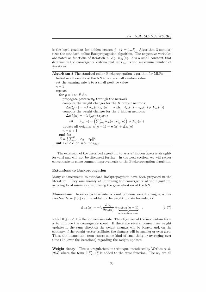
2.8. NEURAL NETWORKS
is the local gradient for hidden neuron j (j = 1..J). Algorithm 3 summa-rizes the standard online Backpropagation algorithm. The respective variablesare noted as functions of iteration n, e.g. wkj(n). ǫ is a small constant thatdetermines the convergence criteria and maxiter is the maximum number ofiterations.
Algorithm 3 The standard online Backpropagation algorithm for MLPs
Initialize all weights of the NN to some small random valueSet the learning rate λ to a small positive valuen = 1repeat
for p = 1 to P do
propagate pattern xp through the networkcompute the weight changes for the K output neurons:
∆wokj(n) = −λ δpk(n) zpj(n) with δpk(n) = epk(n)φ′(Vpk(n))
compute the weight changes for the J hidden neurons:∆wh
ji(n) = −λ δpj(n)xpi(n)
with δpj(n) =(∑K
k=1 δpk(n)wokj(n)
)
φ′(Vpj(n))
update all weights: w(n + 1) = w(n) + ∆w(n)n = n + 1
end for
E = 12
∑Pp=1 ||op − tp||
2
until E < ǫ or n > maxiter
The extension of the described algorithm to several hidden layers is straight-forward and will not be discussed further. In the next section, we will ratherconcentrate on some common improvements to the Backpropagation algorithm.
Extensions to Backpropagation
Many enhancements to standard Backpropagation have been proposed in theliterature. They aim mainly at improving the convergence of the algorithm,avoiding local minima or improving the generalization of the NN.
Momentum In order to take into account previous weight changes, a mo-mentum term [186] can be added to the weight update formula, i.e.
∆wk(n) = −λ∂Ep
∂wk(n)+ α∆wk(n− 1)︸ ︷︷ ︸
momentum term
, (2.57)
where 0 ≤ α < 1 is the momentum rate. The objective of the momentum termis to improve the convergence speed. If there are several consecutive weightupdates in the same direction the weight changes will be bigger, and, on thecontrary, if the weight vector oscillates the changes will be smaller or even zero.Thus, the momentum term causes some kind of smoothing or averaging overtime (i.e. over the iterations) regarding the weight updates.
Weight decay This is a regularization technique introduced by Werbos et al .[257] where the term α
2
∑
x w2x is added to the error function. The wx are all
30
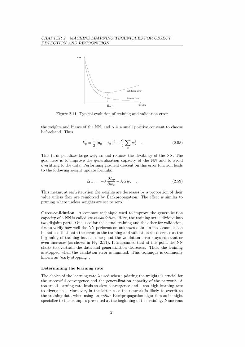
CHAPTER 2. MACHINE LEARNING TECHNIQUES FOR OBJECT
DETECTION AND RECOGNITION
training error
validation error
iteration
error
Emin
Figure 2.11: Typical evolution of training and validation error
the weights and biases of the NN, and α is a small positive constant to choosebeforehand. Thus,
Ep =1
2||op − tp||
2 +α
2
∑
x
w2x . (2.58)
This term penalizes large weights and reduces the flexibility of the NN. Thegoal here is to improve the generalization capacity of the NN and to avoidoverfitting to the data. Performing gradient descent on this error function leadsto the following weight update formula:
∆wx = −λ∂Ep
∂wx
− λα wx . (2.59)
This means, at each iteration the weights are decreases by a proportion of theirvalue unless they are reinforced by Backpropagation. The effect is similar topruning where useless weights are set to zero.
Cross-validation A common technique used to improve the generalizationcapacity of a NN is called cross-validation. Here, the training set is divided intotwo disjoint parts. One used for the actual training and the other for validation,i.e. to verify how well the NN performs on unknown data. In most cases it canbe noticed that both the error on the training and validation set decrease at thebeginning of training but at some point the validation error stays constant oreven increases (as shown in Fig. 2.11). It is assumed that at this point the NNstarts to overtrain the data and generalization decreases. Thus, the trainingis stopped when the validation error is minimal. This technique is commonlyknown as “early stopping”.
Determining the learning rate
The choice of the learning rate λ used when updating the weights is crucial forthe successful convergence and the generalization capacity of the network. Atoo small learning rate leads to slow convergence and a too high learning rateto divergence. Moreover, in the latter case the network is likely to overfit tothe training data when using an online Backpropagation algorithm as it mightspecialize to the examples presented at the beginning of the training. Numerous
31
2.8. NEURAL NETWORKS
solutions for the dynamic adaptation of the learning rate have been proposedin the literature. Most of them focus on the acceleration of the training processrather than their generalization performance. They can roughly be divided intotwo groups: global and local adaption techniques. The former is referring tomethods adjusting an overall learning rate for the whole network and the latterto the adaptation of independent learning rates for each weight.
A method for global adaptation has been proposed by Chan et al . [37] wherethe angle between the last weight update and the current gradient is calculated.If it is less than 90 the learning rate is increased otherwise it is decreased. Sa-lomon et al . [213] proposed an evolutionary based adaption of the learning rate.At each iteration, two weight updates, one with increased and the other withdecreased learning rate, are performed separately. The resulting network thatperforms better is retained and used as a starting point for the next iteration.A heuristic method, the so-called “bold driver” method, has been employedby Battiti et al . [14] and Vogl et al . [255]. Here the learning rate is adjustedaccording to the evolution of the error criteria E. If E decreases the learningrate is slightly increased, otherwise it is drastically decreased. Hsin et al . [102]proposed to use a weighted average of the cosines between successive weight up-dates, and Plagianakos et al . [179] calculated a two point approximation to thesecant equation underlying quasi-Newton methods in order to obtain a dynamiclearning rate and additionally make use of an acceptability condition to ensureconvergence. Finally, the approach of Magoulas et al . [151] estimates the localshape of the error surface by the Lipschitz constant and sets the learning rateaccordingly. They also employed this technique to calculate a separate dynamiclearning rate for each weight [152].
Local learning rate adjustment methods have been very popular due to theirefficiency and generally higher convergence speed. A very well-know techniqueis the Delta-Bar-Delta method introduced by Jacobs et al . [112]. Here, thelearning rates are adjusted according to sign changes of the exponential averagedgradient. Similarly, Silva and Almeida [226] proposed a method where thelearning rates are increased if the respective gradients of the last two iterationshave the same sign and decreased otherwise.
Finally, many methods do not use an explicit learning rate but first calculatea descent gradient direction and then perform a line search (c.f . Alg. 6) suchthat the error criteria is minimized in the direction of the gradient [149, 63, 140].
Note that most of the existing adaptive learning algorithms are offline learn-ing algorithms However, online algorithms generally converge faster when theinput space is large compared to the number of examples (e.g. in image process-ing tasks) or in more complex architectures like Convolutional Neural Networks(CNN) that use shared weights. Thus, for many real world applications theonline Backpropagation algorithm or its variants are still the best choice. Thereare also some adaptive online algorithms in the literature. For example, Schrau-dolph [220], Harmon et al . [95] and Almeida et al . [1] proposed methods similarto the Incremental Delta-Bar-Delta approach introduced by Sutton et al . [232],an extension of the Delta-Bar-Delta technique for online training.
In the following section we will propose a novel approach to learning rateadaption with online Backpropagation. We will show that our algorithm notonly increases convergence speed but also improves the generalization capacityof the resulting NN.
32

CHAPTER 2. MACHINE LEARNING TECHNIQUES FOR OBJECT
DETECTION AND RECOGNITION
A novel approach to learning rate adaption with online Backpropa-
gation
We now introduce a new method to automatically adapt the learning rate ofthe online Backpropagation algorithm [57]. The proposed algorithm requires aseparation of the data set into training and validation set, as described on page31. But here the validation set is not only used for “early stopping” but also tocontrol the learning rate, i.e. to accelerate or decelerate learning. The learningrate is now denoted as a function of n, denoting the iteration, i.e. λ(n). Thus,it is adjusted only after each iteration and not after each training example.
The algorithm consists of two consecutive phases:
1. the main learning phase and
2. the refinement phase.
The main learning phase The adaption of the learning rate in our approachis similar to the “bold driver” method [255, 14] where the learning rate is ini-tialized with a very small value (e.g. 10−10) and adjusted after each trainingiteration according the difference of the error criteria E between the currentand the preceding iteration.
The proposed method applies this idea to the validation set instead of thetraining set in order to reduce overfitting. Moreover, the procedure is slightlymodified to be more tolerant to error increases as the validation error is morelikely to oscillate than the training error. Let us consider the typical shapesof the error curves of a training and validation set when using standard Back-propagation. Fig. 2.11 illustrates this in a simplified manner. When applyingthe technique of “early stopping” the weight configuration at iteration nmin,i.e. where the validation error is minimal, is retained as the network is supposedto show the highest generalization performance at this point. Further train-ing likely leads to overfitting. The purpose of the first phase of the proposedalgorithm is thus to reach the point nmin more quickly.
To this end, the normalized difference between the error criteria of the cur-rent and the preceding iteration is calculated:
δ(n) =Ev(n)− Ev(n− 1)
Ev(n). (2.60)
Ev(n) is the error criteria at iteration n calculated on the whole validationset (c.f . Eq. 2.52).
The algorithm further requires a running average δ(n) of the preceding valuesof δ:
δ(n) = α · δ(n) + (1 − α) · δ(n− 1) , (2.61)
where 0 < α ≤ 1 (e.g. α = 0.1).The principal learning rate updating rule is the following:
λ(n) =
d · λ(n− 1) if δ(n) · δ(n− 1) < 0 and |δ(n− 1)| > θ ,
u · λ(n− 1) otherwise .(2.62)
where u and d are positive constants, 0 < d < 1 < u, and θ is a threshold toallow for small error oscillations. In our experiments we used u = 1.1, d = 0.5
33

2.8. NEURAL NETWORKS
iterationnmin − 1 nminEmin
Ev
(a) The actual minimum has been missed be-
fore iteration nmin
iterationnmin nmin + 1Emin
Ev
(b) The actual minimum has been missed af-
ter iteration nmin
Figure 2.12: The two possible cases that can occur when the minimum on thevalidation set is reached
and θ = 0.01. Thus, the learning rate adaption is based on the signs of theerror differences of the current and the preceding iterations. If the sign changesthe learning rate is decreased, otherwise it is increased. The principle of thisprocedure is similar to the Delta-Bar-Delta method [112] but the calculation isnot based on gradients.
Refinement phase If the training has passed iteration nmin where Ev isminimal the network is likely to overtrain. In fact, as the gradient descent isperformed in discrete steps the actual minimum Emin of the error surface of thevalidation set is likely to be missed and lies between the weight configurationsof two successive training iterations. Fig. 2.12 illustrates this. Clearly, thereare two cases to differentiate: the minimum Emin has been missed either be-fore or after iteration nmin. Now we assume that the validation error surfaceis relatively smooth and that no other local minimum lies between iterationsnmin−1 and nmin or between iterations nmin and nmin +1 respectively. In orderto try to attain a smaller error the network reverts to the weight configurationat iteration nmin − 1, decreases the learning rate, and training is continued.Note that for training only the examples of the training set are used. Thus, itis uncertain if the actual minimum can be attained at all. If no smaller errorhas been found for a certain number of iterations N the “real” minimum, i.e.the minimum on Ev, is more likely to have occurred “after” iteration nmin, (seeFig. 2.12(b)). In this case, the network reverts to iteration nmin, the learningrate is again decreased and training continues. If a smaller error is reachedduring this process, the temporary minimum is retained, and the training con-tinues normally. Otherwise, the reverting procedure is repeated while alwaysretaining the absolute minimum and the respective weight configuration foundso far. Algorithm 4 summarizes the overall training procedure. Note that thecomputational overhead of the algorithm compared to standard Backpropaga-tion with fixed learning rate is negligible as the error on the validation set needsto be calculated anyway if cross-validation is performed.
Fig.2.13 illustrates a typical evolution of the error criteria Ev(n) during thetraining process using the proposed learning algorithm. Due to the initializationwith a very small value, the error stays nearly constant at the beginning but
34

CHAPTER 2. MACHINE LEARNING TECHNIQUES FOR OBJECT
DETECTION AND RECOGNITION
Algorithm 4 The proposed online Backpropagation algorithm with adaptivelearning rate
1: Initialize weights and individual learning rates
2: Set λ(0) := 10−10, δ(0) := 0 and δ(0) := 0
3: Calculate Ev(0)
4: Emin = Ev(0)
5: n := 0
6: repeat
7: Do one training iteration
8: n := n + 1
9: Calculate δ(n) = Ev(n)−Ev(n−1)Ev(n)
10: if δ(n) · δ(n− 1) < 0 and |δ(n− 1)| > θ then
11: λ(n) = d · λ(n− 1)
12: else
13: λ(n) = u · λ(n− 1)
14: end if
15: δ(n) = α · δ(n) + (1− α) · δ(n− 1)
16: if Ev(n) < Emin then
17: save the current weight configuration
18: Emin = Ev(n)
19: nmin := n
20: end if
21: if n− nmin > N then
22: Revert to weight configuration at nmin − 1 (or nmin)
23: end if
24: until n = nmax
drops very quickly at some point due to the exponential increase of the learningrate, and finally it converges to a minimum. In general, the main part of theminimization is done in the first phase, and the error decrease in the refinementphase is relatively small.
In order to validate the approach and to show the benefit compared to stan-dard BP and the basic “bold driver” method we will present some experimentalresults hereafter.
Experimental Results We evaluated the proposed learning algorithm ona MLP trained to classify the examples of the well-known NIST database ofhandwritten digits. The database contains 3823 training and 1797 test examplesof 8x8 matrices. From the training set 500 examples were selected randomlyand used for validation. The MLP we used for the experiments had 64 input,10 hidden and 10 output neurons, fully inter-connected. The neurons all hadsigmoid activation functions.
To ensure that the neural network is well-conditioned, we additionally usedfixed local learning rates that were distributed stepwise from the last layer to
35
2.8. NEURAL NETWORKS
refinementmain learning
0
0.2
0.4
0.6
0.8
1
0 100 200 400 500 600iteration
300
Ev
Figure 2.13: A typical evolution of the error criteria on the validation set usingthe proposed learning algorithm
the first layer according to the incoming connections of each neuron. Thus, theoutput neurons had the highest and the input the lowest local learning rate.The overall learning rate is just the product of the fixed local and the dynamicglobal learning rate.
In the first experiment, we compared the convergence properties of the pro-posed algorithm to the ones of standard Backpropagation. Fig. 2.14 shows theresulting error curves evaluated on the validation set. The different curves forthe Backpropagation algorithm have been obtained by using different globallearning rates (10−3, 10−4 and 10−5). The global learning rate of the proposedmethod was initialized with the value 10−7. Note that our approach convergesmore slowly at the beginning but catches up quickly and finishes stable on thesame level or even lower than Backpropagation.
Fig. 2.15 illustrates that our method is not sensitive to different initializa-tions of the global learning rate. The curves show the validation error curves forthree different runs with initial learning rates of 10−6, 10−8 and 10−10 respec-tively. Note that the point of time where the minimum is reached increases onlylinearly when the initial learning rate is decreased exponentially. This is anotherside effect of the exponential learning rate update rule. All the runs converge toapproximately the same solution, and the recognition rates are about the samefor all networks.
The final experiment demonstrates that the algorithm not only convergesfaster but also improves the generalization performance of the resulting neuralnetworks. To this end, the training set was gradually reduced and the respectiverecognition rates on the test set were calculated and compared to the standardBackpropagation as well as to the bold driver method [255, 14]. Table 2.1 showsthe overall results. One can see that the proposed method performs slightlybetter with training set sizes 3323 and 1000 and clearly outperforms the otheralgorithms when only 600 and 100 training examples are used.
Table 2.2 shows the respective results with a neural network with 40 hiddenneurons. The recognition rates of the proposed method are slightly better thenfor the other algorithms, although the difference is less significant than with
36

CHAPTER 2. MACHINE LEARNING TECHNIQUES FOR OBJECT
DETECTION AND RECOGNITION
0
0.2
0.4
0.6
0.8
1
0 200 400 600 800 1000
iteration
Ev
Backpropagation (LR = 10−5)Backpropagation (LR = 10−4)Backpropagation (LR = 10−3)
proposed algorithm (LR = 10−7)
Figure 2.14: The evolution of the validation error on the NIST database usingBackpropagation and the proposed algorithm
0
0.1
0.2
0.3
0.4
0.5
0.6
0.7
0.8
0.9
0 100 200 300 400 500 600
iteration
Ev
10−6
10−8
10−10
Figure 2.15: The validation error curves of the proposed approach with differentinitial global learning rates
training set size 3323 1000 600 100algorithm
Backpropagation 94.30 93.42 78.31 73.88bold driver [255, 14] 93.41 91.32 83.74 72.75proposed algorithm 94.50 93.71 85.29 78.10
Table 2.1: Recognition rate (in %) with varying training set size (10 hiddenneurons)
37
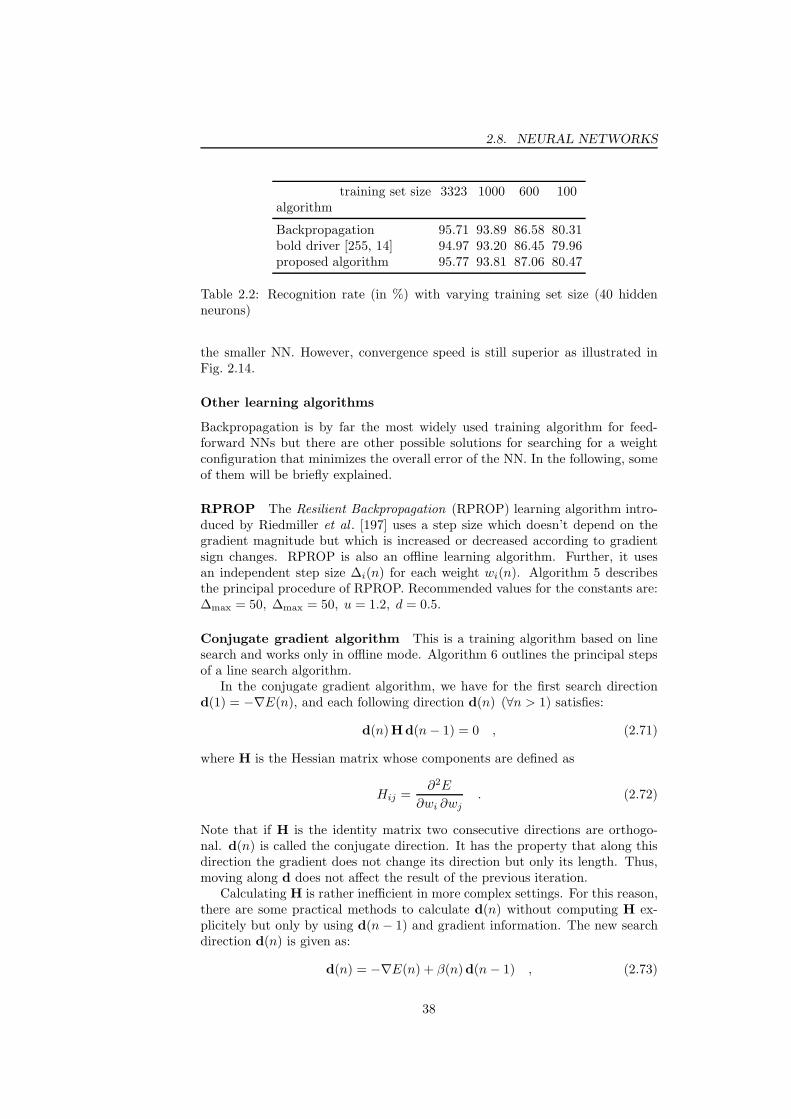
2.8. NEURAL NETWORKS
training set size 3323 1000 600 100algorithm
Backpropagation 95.71 93.89 86.58 80.31bold driver [255, 14] 94.97 93.20 86.45 79.96proposed algorithm 95.77 93.81 87.06 80.47
Table 2.2: Recognition rate (in %) with varying training set size (40 hiddenneurons)
the smaller NN. However, convergence speed is still superior as illustrated inFig. 2.14.
Other learning algorithms
Backpropagation is by far the most widely used training algorithm for feed-forward NNs but there are other possible solutions for searching for a weightconfiguration that minimizes the overall error of the NN. In the following, someof them will be briefly explained.
RPROP The Resilient Backpropagation (RPROP) learning algorithm intro-duced by Riedmiller et al . [197] uses a step size which doesn’t depend on thegradient magnitude but which is increased or decreased according to gradientsign changes. RPROP is also an offline learning algorithm. Further, it usesan independent step size ∆i(n) for each weight wi(n). Algorithm 5 describesthe principal procedure of RPROP. Recommended values for the constants are:∆max = 50, ∆max = 50, u = 1.2, d = 0.5.
Conjugate gradient algorithm This is a training algorithm based on linesearch and works only in offline mode. Algorithm 6 outlines the principal stepsof a line search algorithm.
In the conjugate gradient algorithm, we have for the first search directiond(1) = −∇E(n), and each following direction d(n) (∀n > 1) satisfies:
d(n)Hd(n− 1) = 0 , (2.71)
where H is the Hessian matrix whose components are defined as
Hij =∂2E
∂wi ∂wj
. (2.72)
Note that if H is the identity matrix two consecutive directions are orthogo-nal. d(n) is called the conjugate direction. It has the property that along thisdirection the gradient does not change its direction but only its length. Thus,moving along d does not affect the result of the previous iteration.
Calculating H is rather inefficient in more complex settings. For this reason,there are some practical methods to calculate d(n) without computing H ex-plicitely but only by using d(n− 1) and gradient information. The new searchdirection d(n) is given as:
d(n) = −∇E(n) + β(n)d(n− 1) , (2.73)
38

CHAPTER 2. MACHINE LEARNING TECHNIQUES FOR OBJECT
DETECTION AND RECOGNITION
Algorithm 5 The RPROP algorithm
1: n = 12: ∆i(1) = ∆min ∀i = 1..N3: repeat
4: Perform forward propagation of every example while accumulating∇E(n)5: for i = 0 to N do
6: Update the step sizes:
∆i(n) = ∆i(n− 1) · u if∂E(n)
∂wi(n)·
∂E(n− 1)
∂wi(n− 1)> 0 (2.63)
∆i(n) = ∆i(n− 1) · d if∂E(n)
∂wi(n)·
∂E(n− 1)
∂wi(n− 1)< 0 (2.64)
∆i(n) = ∆max if ∆i(n) ≥ ∆max (2.65)
∆i(n) = ∆min if ∆i(n) ≤ ∆min (2.66)
7: Update the weights:
if∂E(n)∂wi(n) ·
∂E(n−1)∂wi(n−1) ≥ 0 then
∆wi(n) = −∆i(n) if∂E(n)
∂wi(n)> 0 (2.67)
∆wi(n) = +∆i(n) if∂E(n)
∂wi(n)< 0 (2.68)
8: else
∆wi(n) = 0 (2.69)
9: end if
10:
wi(n) = wi(n− 1) + ∆wi(n) (2.70)
11: end for
12: until E < ǫ
Algorithm 6 The line search algorithm
1: n=12: repeat
3: Determine a search direction d(n)4: Minimize E(n) w.r.t. a factor λ by modifying the weight vector w(n)
along the search direction, i.e. w(n) = w(n)+λd. Let λopt be this value.5: Update the weight vector: w(n + 1) = w(n) + λopt d
6: n = n + 17: until E < ǫ (ǫ being a small positive constant)
39

2.8. NEURAL NETWORKS
where β(n) can be calculated by using, for example, the Fletcher-Reeves for-mula:
β(n) =∇E(n)T∇E(n)
∇E(n− 1)T∇E(n− 1)(2.74)
or the Polak-Ribiere formula:
β(n) =(∇E(n)−∇E(n− 1))T∇E(n)
∇E(n− 1)T∇E(n− 1). (2.75)
It has been shown that in case of a quadratic polynomial error function thealgorithm converges in N steps, where N is the number of weight parameters.However, in most applications the error function is not quadratic, hence theconvergence is slower.
Newton algorithm In Newton’s method the error surface E is assumed tobe quadratic polynomial. Then, the minimum of E can be reached in one step(the so-called Newton step):
∆w = −H−1∇E , (2.76)
where H is the Hessian matrix (c.f . Eq. 2.72). However, as E is usually non-quadratic only a small step in this direction is performed, and H is computedwith the new weight configuration. Thus, at each iteration we calculate,
∆w = −λH−1∇E , (2.77)
where 0 < λ < 1.In most applications, the basic Newton’s algorithm is impractical because of
the following reasons:
• H has to be positive definite in order to allow calculating its inverse.However, this is not always the case.
• A N × N matrix must be stored and inverted at each iteration which isof O(N3) computational complexity.
• The quadratic local approximation of E is often two imprecise such thatλ has to be chosen very small.
A partial solution to this presents the Broyden-Fletcher-Goldfarb-Shanno(BFGS) method or Quasi-Newton method [188]. The authors propose to ap-proximate H−1 iteratively by only using first order gradient information. How-ever, the algorithm still needs to store a N ×N matrix and the computationalcomplexity is O(N2). Further, LeCun et al . [138] presented a method to iter-atively estimate the largest eigenvalue of H and also showed that the optimallearning rate λ is approximately the inverse of this value.
2.8.6 Radial Basis Function Networks
Introduction
The idea behind Radial Basis Function (RBF) Networks, shortly RBF, is basedon Cover’s theorem [48]:
40

CHAPTER 2. MACHINE LEARNING TECHNIQUES FOR OBJECT
DETECTION AND RECOGNITION
input RBFs output
X
Tj
yk
Figure 2.16: The architecture of a RBF Network
“A complex pattern-classification problem cast in a high-dimensionalspace nonlinearly is more likely to be linearly separable than in alow-dimensional space.”
Powell [187] introduced RBFs as a solution to the real multivariate interpola-tion problem but Broomhead and Lowe [30] were the first to exploit the use ofRBFs in the context of NNs. They have been applied to many real-world prob-lems since then, notably in the fields of functional approximation, time-seriesmodeling and pattern classification.
RBF Networks are three-layer feed-forward NNs similar to MLPs, i.e. theyconsist of
• an input layer having no weights and receiving the input pattern,
• a hidden layer implementing the non-linear RBFs and fully connected tothe input layer,
• an output layer consisting of perceptrons with linear activation functions.
Figure 2.16 illustrates the principal architecture of RBF Networks.The principal difference to MLPs are the hidden neurons performing a non-
linear mapping onto a subspace which is characterized by the RBFs that areparameterized by the respective neurons.
Thus, for a RBF Network having I inputs, J hidden neurons and K outputs,the outputs yk are are calculated as follows:
yk =
J∑
j=0
wkjΦj(||X −Tj||) , (2.78)
where wkj is the weight from hidden neuron j to output neuron k, Φj is theRBF integrated by hidden neuron j with center Tj ∈ R
I , X ∈ RI is the input
41

2.8. NEURAL NETWORKS
vector, and || · || represents some norm, in general the L1 or L2 norm. Φ0 canbe set to 1 in order to use bias terms (i.e. wk0). As can be noticed, the outputof a hidden neuron j depends on the distance of X from the neuron’s center Tj,a distance of zero leading to a maximum or minimum activation according tothe function Φj chosen.
The most common RBF is the Gaussian function:
Φj(||X−Tj||) = exp[−(X−Tj)
T Σ−1j (X−Tj)
], (2.79)
Σj being the covariance matrix which determines the shape, size and orientationof the receptive field of the neuron j, i.e. a subspace of the input space whereΦj is having a higher activation. For example, for a diagonal covariance matrixwith equal diagonal elements the receptive field is a hypersphere centered at Tj;in the general case it is a hyperellipsoid.
Training
As MLPs, RBF Networks are trained using an labeled training data set and byadjusting its parameters such that an error function is minimized. In most ofthe cases, the error function is the sum over all training examples of the squareddistances between the NN output and the desired output (see Eq. 2.52).
However, different training strategies can be adopted w.r.t. the hidden layer:
1. use fixed Gaussian RBFs chosen at random
2. use RBFs with fixed variance and adjust their centers by an unsupervisedlearning algorithm
3. adjust centers and variances of the RBFs by a supervised learning algo-rithm.
In the first case, the only parameters to learn are the weights and the biasesof the output neurons. This can be done for example by the Least-Mean-Squares(LMS) algorithm or Error Backpropagation (c.f . Algorithm 3).
The second learning strategy consists of two stages. In the first stage, thecenters of the RBFs are initialized randomly and then determined iterativelyby a clustering algorithm, such as k-means, Linear Vector Quantization (LVQ)or Self-Organizing Maps (SOM). The variances are then computed using thevariances of the respective clusters. In the second stage, the weights of theoutput neurons are calculated by a supervised learning algorithm.
The third learning strategy is completely supervised, i.e. the centers, thecovariance matrix and the weights of the output neurons are adjusted iterativelyby offline Backpropagation.
2.8.7 Self-Organizing Maps
Introduction
The NNs discussed so far are all used for supervised learning. Self-OrganizingMaps (SOM) however rely on an unsupervised learning algorithm and are usedwhen the structure of the training data is unknown. This approach has beenproposed by Willshaw, von der Malsburg [258] and Kohonen [123]. The idea is toproject high-dimensional input vectors onto a low-dimensional map (mostly 1D,
42
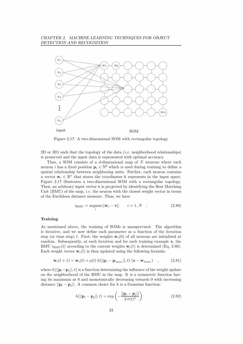
CHAPTER 2. MACHINE LEARNING TECHNIQUES FOR OBJECT
DETECTION AND RECOGNITION
...x1
x2
x3
x4
xn
w1 w2
wN
input SOM
Figure 2.17: A two-dimensional SOM with rectangular topology
2D or 3D) such that the topology of the data (i.e. neighborhood relationships)is preserved and the input data is represented with optimal accuracy.
Thus, a SOM consists of a d-dimensional map of N neurons where eachneuron i has a fixed position pi ∈ N
d which is used during training to define aspatial relationship between neighboring units. Further, each neuron containsa vector wi ∈ R
n that stores the coordinates it represents in the input space.Figure 2.17 illustrates a two-dimensional SOM with a rectangular topology.Then, an arbitrary input vector v is projected by identifying the Best MatchingUnit (BMU) of the map, i.e. the neuron with the closest weight vector in termsof the Euclidean distance measure. Thus, we have
iBMU = argmini
||wi − v|| i = 1..N . (2.80)
Training
As mentioned above, the training of SOMs is unsupervised. The algorithmis iterative, and we now define each parameter as a function of the iterationstep (or time step) t. First, the weights wi(0) of all neurons are initialized atrandom. Subsequently, at each iteration and for each training example x, theBMU iBMU(t) according to the current weights wi(t) is determined (Eq. 2.80).Each weight vector wi(t) is then updated using the following formula:
wi(t + 1) = wi(t) + ρ(t) h(||pi − piBMU ||, t) (x−wiBMU) , (2.81)
where h(||pi−pj||, t) is a function determining the influence of the weight updateon the neighborhood of the BMU in the map. It is a symmetric function hav-ing its maximum at 0 and monotonically decreasing towards 0 with increasingdistance ||pi − pj ||. A common choice for h is a Gaussian function:
h(||pi − pj ||, t) = exp
(
−||pi − pj ||
2 σ(t)2
)
(2.82)
43
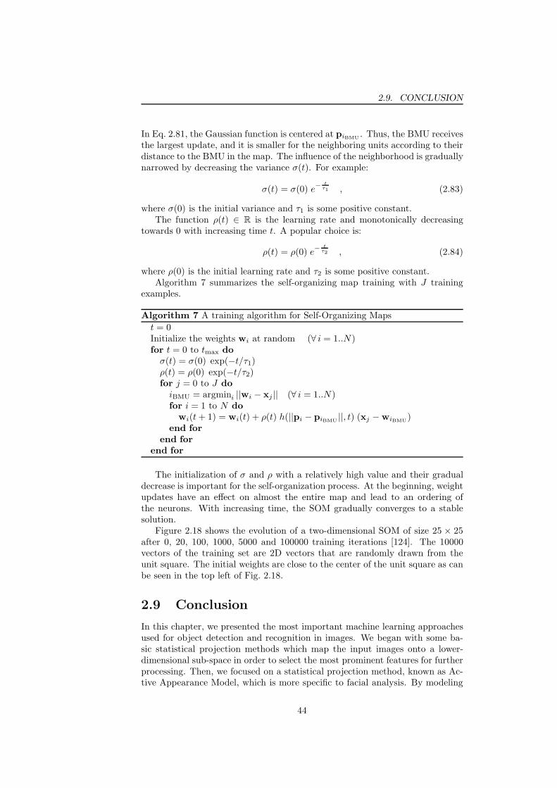
2.9. CONCLUSION
In Eq. 2.81, the Gaussian function is centered at piBMU . Thus, the BMU receivesthe largest update, and it is smaller for the neighboring units according to theirdistance to the BMU in the map. The influence of the neighborhood is graduallynarrowed by decreasing the variance σ(t). For example:
σ(t) = σ(0) e−t
τ1 , (2.83)
where σ(0) is the initial variance and τ1 is some positive constant.The function ρ(t) ∈ R is the learning rate and monotonically decreasing
towards 0 with increasing time t. A popular choice is:
ρ(t) = ρ(0) e−t
τ2 , (2.84)
where ρ(0) is the initial learning rate and τ2 is some positive constant.Algorithm 7 summarizes the self-organizing map training with J training
examples.
Algorithm 7 A training algorithm for Self-Organizing Maps
t = 0Initialize the weights wi at random (∀ i = 1..N)for t = 0 to tmax do
σ(t) = σ(0) exp(−t/τ1)ρ(t) = ρ(0) exp(−t/τ2)for j = 0 to J do
iBMU = argmini ||wi − xj || (∀ i = 1..N)for i = 1 to N do
wi(t + 1) = wi(t) + ρ(t) h(||pi − piBMU ||, t) (xj −wiBMU)end for
end for
end for
The initialization of σ and ρ with a relatively high value and their gradualdecrease is important for the self-organization process. At the beginning, weightupdates have an effect on almost the entire map and lead to an ordering ofthe neurons. With increasing time, the SOM gradually converges to a stablesolution.
Figure 2.18 shows the evolution of a two-dimensional SOM of size 25 × 25after 0, 20, 100, 1000, 5000 and 100000 training iterations [124]. The 10000vectors of the training set are 2D vectors that are randomly drawn from theunit square. The initial weights are close to the center of the unit square as canbe seen in the top left of Fig. 2.18.
2.9 Conclusion
In this chapter, we presented the most important machine learning approachesused for object detection and recognition in images. We began with some ba-sic statistical projection methods which map the input images onto a lower-dimensional sub-space in order to select the most prominent features for furtherprocessing. Then, we focused on a statistical projection method, known as Ac-tive Appearance Model, which is more specific to facial analysis. By modeling
44
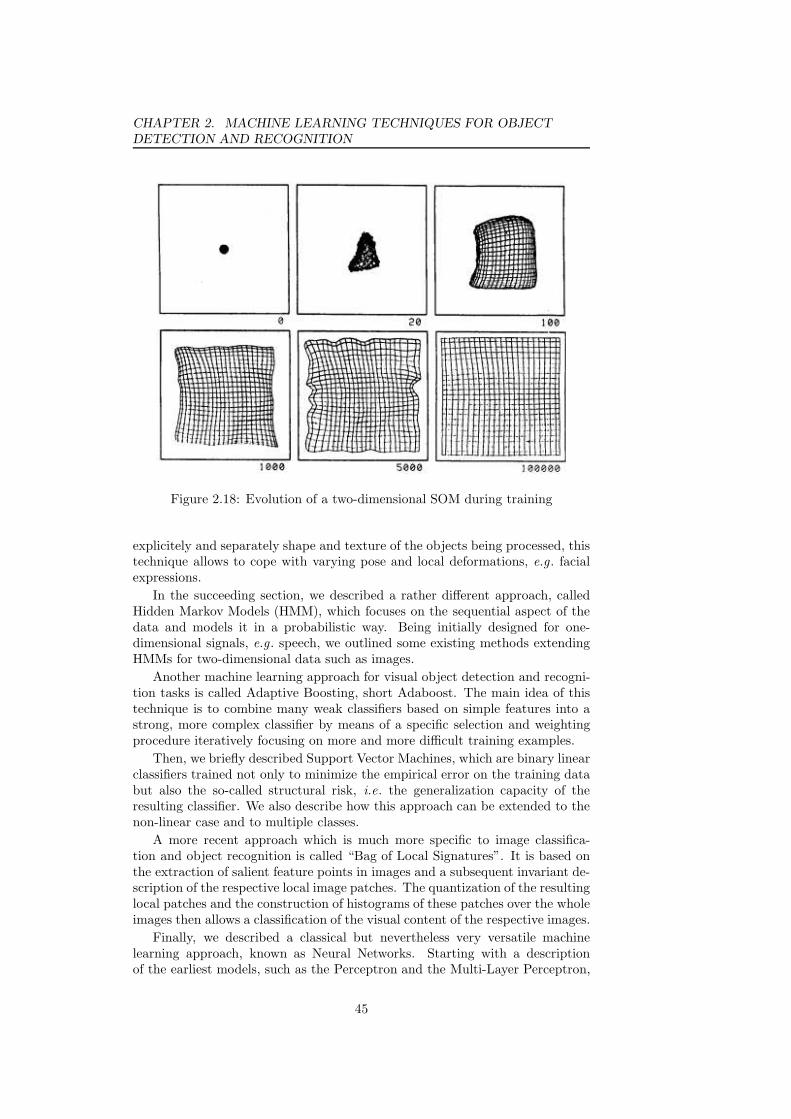
CHAPTER 2. MACHINE LEARNING TECHNIQUES FOR OBJECT
DETECTION AND RECOGNITION
Figure 2.18: Evolution of a two-dimensional SOM during training
explicitely and separately shape and texture of the objects being processed, thistechnique allows to cope with varying pose and local deformations, e.g. facialexpressions.
In the succeeding section, we described a rather different approach, calledHidden Markov Models (HMM), which focuses on the sequential aspect of thedata and models it in a probabilistic way. Being initially designed for one-dimensional signals, e.g. speech, we outlined some existing methods extendingHMMs for two-dimensional data such as images.
Another machine learning approach for visual object detection and recogni-tion tasks is called Adaptive Boosting, short Adaboost. The main idea of thistechnique is to combine many weak classifiers based on simple features into astrong, more complex classifier by means of a specific selection and weightingprocedure iteratively focusing on more and more difficult training examples.
Then, we briefly described Support Vector Machines, which are binary linearclassifiers trained not only to minimize the empirical error on the training databut also the so-called structural risk, i.e. the generalization capacity of theresulting classifier. We also describe how this approach can be extended to thenon-linear case and to multiple classes.
A more recent approach which is much more specific to image classifica-tion and object recognition is called “Bag of Local Signatures”. It is based onthe extraction of salient feature points in images and a subsequent invariant de-scription of the respective local image patches. The quantization of the resultinglocal patches and the construction of histograms of these patches over the wholeimages then allows a classification of the visual content of the respective images.
Finally, we described a classical but nevertheless very versatile machinelearning approach, known as Neural Networks. Starting with a descriptionof the earliest models, such as the Perceptron and the Multi-Layer Perceptron,
45

2.9. CONCLUSION
and the way they can be trained we then outlined some more specific neuralapproaches being used for image processing tasks, i.e. Auto-Associative NeuralNetworks, Radial Basis Function Networks and Self-Organizing Maps.
A neural network approach showing to be particularly appropriate for visualobject detection and recognition tasks and being inspired by biological evidencein the visual system of mammals is called Convolutional Neural Network. Beingthe foundation of the methods proposed in this work, we will describe thisapproach in more detail in the following chapter.
46
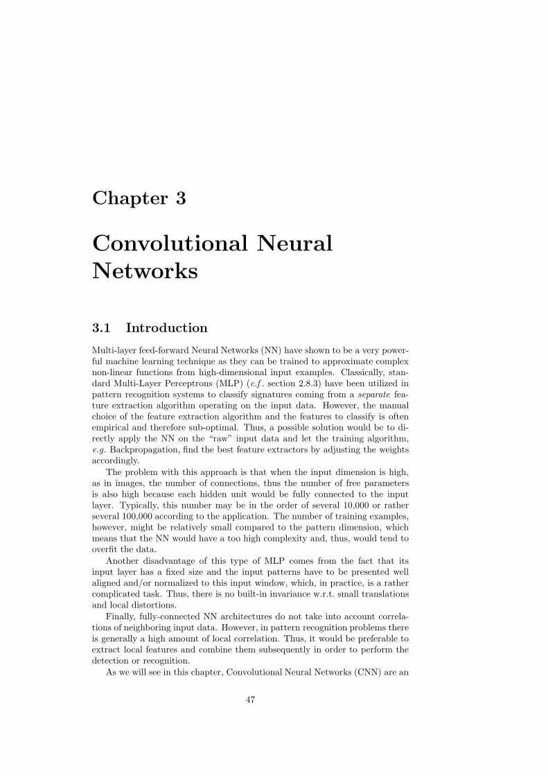
Chapter 3
Convolutional Neural
Networks
3.1 Introduction
Multi-layer feed-forward Neural Networks (NN) have shown to be a very power-ful machine learning technique as they can be trained to approximate complexnon-linear functions from high-dimensional input examples. Classically, stan-dard Multi-Layer Perceptrons (MLP) (c.f . section 2.8.3) have been utilized inpattern recognition systems to classify signatures coming from a separate fea-ture extraction algorithm operating on the input data. However, the manualchoice of the feature extraction algorithm and the features to classify is oftenempirical and therefore sub-optimal. Thus, a possible solution would be to di-rectly apply the NN on the “raw” input data and let the training algorithm,e.g. Backpropagation, find the best feature extractors by adjusting the weightsaccordingly.
The problem with this approach is that when the input dimension is high,as in images, the number of connections, thus the number of free parametersis also high because each hidden unit would be fully connected to the inputlayer. Typically, this number may be in the order of several 10,000 or ratherseveral 100,000 according to the application. The number of training examples,however, might be relatively small compared to the pattern dimension, whichmeans that the NN would have a too high complexity and, thus, would tend tooverfit the data.
Another disadvantage of this type of MLP comes from the fact that itsinput layer has a fixed size and the input patterns have to be presented wellaligned and/or normalized to this input window, which, in practice, is a rathercomplicated task. Thus, there is no built-in invariance w.r.t. small translationsand local distortions.
Finally, fully-connected NN architectures do not take into account correla-tions of neighboring input data. However, in pattern recognition problems thereis generally a high amount of local correlation. Thus, it would be preferable toextract local features and combine them subsequently in order to perform thedetection or recognition.
As we will see in this chapter, Convolutional Neural Networks (CNN) are an
47

3.2. BACKGROUND
input
input outputexcitatory
inhibitory
u(1)
u(2)
u(3)
u(4)
u(5)
u(6)
a(1)
a(2)
a(3)
a(4)
a(5)
a(6)
vb
e
h
1+e1+h− 1 X
X
W
φ W = φ(X)Σ
Figure 3.1: The model of a S-cell used in the Neocognitron
approach that tries to alleviate the above mentioned problems. That is, theyautomatically learn local feature extractors, they are invariant to small transla-tions and distortions in the input pattern, and they implement the principle ofweight sharing which drastically reduces the number of free parameters and thusincreases their generalization capacity compared to NN architectures withoutthis property.
3.2 Background
3.2.1 Neocognitron
The first implementation of a CNN was the so-called Neocognitron proposed byFukushima [74, 75, 76, 77] which has been originally applied to the problem ofhandwritten digit recognition. The Neocognitron makes use of receptive fields,i.e. each neuron is only connected to a sub-region corresponding to a certainnumber of neighboring neurons, in the preceding layer. This idea has beeninspired by the discovery of locally-sensitive, orientation-selective neurons in thecat’s visual system by Hubel and Wiesel [106]. Local connections have been usedmany times with NNs [73, 133, 167]. They can be used to detect elementaryvisual features in images, such as oriented edges, end points or corners. Asone feature extractor can be useful in several parts of the input image, theweights are forced to be identical for all possible locations of the receptive field,a principal called weight sharing [208].
The outputs of the respective neurons with identical weights, the so-calledS-cells, form a S-plane. Fig. 3.1 illustrates the model of a S-cell. Note thatbesides the input from the receptive field, called excitatory input e, there isalso an inhibitory input h which has a negative effect on the activation of theneuron. If h is greater than e the output of the neuron is zero. The excitatoryinput is calculated as follows:
e =
N∑
i=1
a(i) u(i) , (3.1)
48

CHAPTER 3. CONVOLUTIONAL NEURAL NETWORKS
where a(i) are the training weights, u(i) denote the inputs from the precedingcells, and N is the number of weights. For the inhibitory input, we have:
h = b v , (3.2)
where b is a trainable weight. In the Neocognitron, the input v is calculated asthe weighted root mean-squared values coming from the receptive field and thusrepresents some kind of normalization. Finally, the activation of a S-cell is:
uS(i) = φ
(1 + e
1 + h− 1
)
, (3.3)
where the activation function φ is defined as:
φ(X) =
X if X ≥ 00 otherwise
(3.4)
Fukushima [76] showed that the outputs of the S-cells approximate a convo-lution normalized by the length of the weight vector and the input vector. Sev-eral S-planes, each containing a different set of weights, can be used to extractdifferent features at the same locations. The set of S-planes at one particularlevel form a S-layer.
The exact position of each feature is not very important in most cases.Therefore, each S-plane is followed by a C-plane which reduce the resolution ofthe respective S-plane by a constant factor, e.g. two and thus performs a kindof sub-sampling or blurring. The sub-sampling also reduces the sensitivity ofthe NN to small shifts and distortions of the input pattern.
By alternating C-layers and S-layers and combining the outputs of the re-spective maps, one can construct more complex feature extractors. This princi-ple was inspired by Hubel and Wiesel’s notion of “simple” and “complex” cellsand it has been implemented in the Neocognitron where the first S-planes extractsimple visual features, such as oriented edges or corner points, and the followinglayers combine them to extract more complex features, such as combinations ofline segments.
The topology of the basic Neocognitron is illustrated in Fig. 3.2. It hasan input layer uC0 and four alternating S- and C-layers, uS1, uC1, . . . , uS4, uC4,where uC4 is the output layer consisting of single neurons representing the de-cision of the NN for some input pattern, in this case a digit. Note that theinhibitory inputs v are not depicted in Fig. 3.2. In fact, all inhibitory inputsof the S-planes of one layer uSi are connected to a so-called V-plane uV i. TheV-neurons of each V-plane receive their inputs from corresponding sub-regionsin each preceding C-plane. The output is the weighted root mean square ofthese values and form the input v of the S-cells at the respective positions.
The training of the Neocognitron can be supervised or unsupervised. Thefirst implementations used an unsupervised training algorithm based on self-or-ganization and a particular reinforcement learning rule. However, later studiesshowed that the performance of the Neocognitron trained with a supervisedalgorithm was higher than with the original self-organization method. Further,training is performed layer by layer, i.e. starting from the first S-layer uS1 untilthe output layer uC4, such that the training of a particular layer is only startedafter the training of the previous layer is finished. A reinforcement technique is
49

3.2. BACKGROUND
. . .
. . .
. . .
. . .
. . .
. . .
. . .
. . .
uC0
uS1 uC1uS2
uC2 uS3uC3 uS4
uC4
a1
d1
receptive field
Figure 3.2: The topology of the basic Neocognitron
employed by the supervised algorithm in order to train each plane in a layer todetect a specific visual feature, e.g. a horizontal edge. The trainable parametersare the weights a and b, whereas the weights of the C-planes are not modifiedby the training algorithm and fixed at the beginning. At each step, the inputpattern is propagated until the layer that is currently learned. For example, withhandwritten digit recognition, the first layer is trained to recognize some verysimple 3 × 3 pixel patterns, representing oriented edges (see Fig. 3.3(a)). Thesecond layer is then trained to detect some more complex feature, e.g. orientedline end points, corner points or combinations of oriented line segments (seeFig. 3.3(b)). Each S-plane learns a particular pattern. The following S-layersare trained to recognize more and more complex features until the final S-layeruS4, the planes of which are supposed to recognize the whole digit patterns.
The complete description of the rather complex Neocognitron would be be-yond the scope of this work, and we refer to the literature [73, 74, 75, 76, 77]for further details. Fukushima presented many extensions to the basic modeldescribed here. For example, a non-linear activation function φ or the conceptof selective attention [75], where there are not only forward but also backwardconnections of the layers and also interactions between the different planes of alayer controlling the learning process.
3.2.2 LeCun’s Convolutional Neural Network model
An important breakthrough of CNNs came with the widespread use of the Back-propagation learning algorithm (c.f . section 2.8.5) for multi-layer feed-forwardNNs. LeCun et al . [134] presented the first CNN that was trained by Backprop-agation and applied it to the problem of handwritten digit recognition. As thismodel forms the basis of all the NN architectures presented in this work we willdescribe it in more detail in this section. From now on, when we employ theterm Convolutional Neural Network we principally refer to NN models that aresimilar to the one proposed by LeCun et al . [134], which is actually a simplermodel than the Neocognitron and its extensions.
50
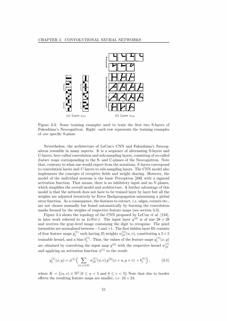
CHAPTER 3. CONVOLUTIONAL NEURAL NETWORKS
(a) Layer uS1 (b) Layer uS2
Figure 3.3: Some training examples used to train the first two S-layers ofFukushima’s Neocognitron. Right: each row represents the training examplesof one specific S-plane
Nevertheless, the architecture of LeCun’s CNN and Fukushima’s Neocog-nitron resemble in many aspects. It is a sequence of alternating S-layers andC-layers, here called convolution and sub-sampling layers, consisting of so-calledfeature maps corresponding to the S- and C-planes of the Neocognitron. Notethat, contrary to what one would expect from the notations, S -layers correspondto convolution layers and C -layers to sub-sampling layers. The CNN model alsoimplements the concepts of receptive fields and weight sharing. However, themodel of the individual neurons is the basic Perceptron [200] with a sigmoidactivation function. That means, there is no inhibitory input and no V-planes,which simplifies the overall model and architecture. A further advantage of thismodel is that the network does not have to be trained layer by layer but all theweights are adjusted iteratively by Error Backpropagation minimizing a globalerror function. As a consequence, the features to extract, i.e. edges, corners etc.,are not chosen manually but found automatically by learning the convolutionmasks formed by the weights of respective feature maps (see section 3.3).
Figure 3.4 shows the topology of the CNN proposed by LeCun et al . [134],in later work referred to as LeNet-1. The input layer y(0) is of size 28 × 28and receives the gray-level image containing the digit to recognize. The pixelintensities are normalized between−1 and +1. The first hidden layer H1 consists
of four feature maps y(1)j each having 25 weights w
(1)j0 (u, v), constituting a 5× 5
trainable kernel, and a bias b(1)j . Thus, the values of the feature maps y
(1)j (x, y)
are obtained by convolving the input map y(0) with the respective kernel w(1)j0
and applying an activation function φ(1) to the result:
y(1)j (x, y) = φ(1)
( ∑
(u,v)∈K
w(1)j0 (u, v) y(0)(x + u, y + v) + b
(1)j
)
, (3.5)
where K = (u, v) ∈ N2 | 0 ≤ u < 5 and 0 ≤ v < 5 Note that due to border
effects the resulting feature maps are smaller, i.e. 24× 24.
51

3.2. BACKGROUND
. . .
input layer
output layerH1 H2
H3 H4
Figure 3.4: The architecture of the CNN proposed by LeCun et al . [134] forhandwritten digit recognition (LeNet-1)
Each convolution map is followed by a sub-sampling map y(2)j which performs
a kind of averaging and reduces the dimension of the respective convolution mapby a factor two. Hence, the sub-sampling maps of layer H2 are of size 12× 12.
Further, each sub-sampling map has a weight w(2)j and a bias b
(2)j . Thus,
y(2)j (x, y) = φ(2)
(
w(2)j ×
∑
(u,v)∈0,12
y(1)j (2x + u, 2y + v) + b
(2)j
)
. (3.6)
φ(2) again is an activation function which has to be continuous and differentiableas required by the Backpropagation learning algorithm.
Figure 3.5 illustrates the process of convolution and sub-sampling.Layers H3 and H4, each contain 12 convolution and sub-sampling maps of
dimensions 8×8 and 4×4 respectively. The function they implement is exactly
convolution 5x5
subsampling
Figure 3.5: An input image followed by a feature map performing a 5 × 5convolution and a 2× 2 sub-sampling map
52

CHAPTER 3. CONVOLUTIONAL NEURAL NETWORKS
the same as the layers H1 and H2 except that the feature maps of layer H3perform a 3 × 3 convolution instead of a 5 × 5. Further, one convolution map
j in layer H3 can have several kernels w(3)ji operating on different maps i in the
preceding layer H2. The activation of respective convolution maps is then simplythe sum of all convolution results and the bias. Thus, the general activationformula for a convolution map j in layer l is:
y(l)j (x, y) = φ(l)
(∑
i∈I
∑
(u,v)∈K
w(l)ji (u, v) y
(l−1)i (x + u, y + v) + b
(l)j
)
, (3.7)
where K = (u, v) ∈ N2 | 0 ≤ u < sx ; 0 ≤ v < sy, (sx, sy) is the dimension
of the convolution kernel, and I is the set of maps of the preceding layer theconvolution map j is connected to. The feature maps in layer H3 learn to extractmore complex features by combining the extracted simple features of layer H2.The connection scheme is illustrated in Fig. 3.4.
Finally, the output layer contains a set of 10 neurons, fully connected tothe previous sub-sampling maps of layer H4, and representing the 10 digits torecognize. The “winning” neuron is supposed to respond with the value +1 andthe other neurons with −1.
In total, the network has 4635 units, 98442 connections, but, due to weightsharing, only 2578 independent parameters to learn.
3.3 Training Convolutional Neural Networks
The training of CNNs is very similar to the training of other types of NNs, suchas ordinary MLPs. A set of training examples is required, and it is preferableto have a separate validation set in order to perform cross-validation and “earlystopping” and to avoid overtraining (see section 2.8.5).
To improve generalization, small transformations, such as shift and distor-tion, can be manually applied to the training set. Consequently the set isaugmented by examples that are artificial but still form valid representations ofthe respective object to recognize. In this way, the CNN learns to be invariantto these types of transformations.
In terms of the training algorithm, in general, online Error Backpropagationleads to the best performance of the resulting CNN. Therefore, this algorithmhas been applied for all experiments throughout this work, and it will be de-scribed in detail in the following section. In section 3.3.2, we will also outlinesome alternatives published in the literature.
3.3.1 Error Backpropagation with Convolutional Neural
Networks
As the online Backpropagation algorithm is the most commonly used learningalgorithm for CNNs it will be described in more detail in this section. In fact,it is almost identical to the Backpropagation algorithm for standard MLPs (seesection 2.8.5). The only difference to take into account is the weight sharing inthe convolution and sub-sampling layers.
53
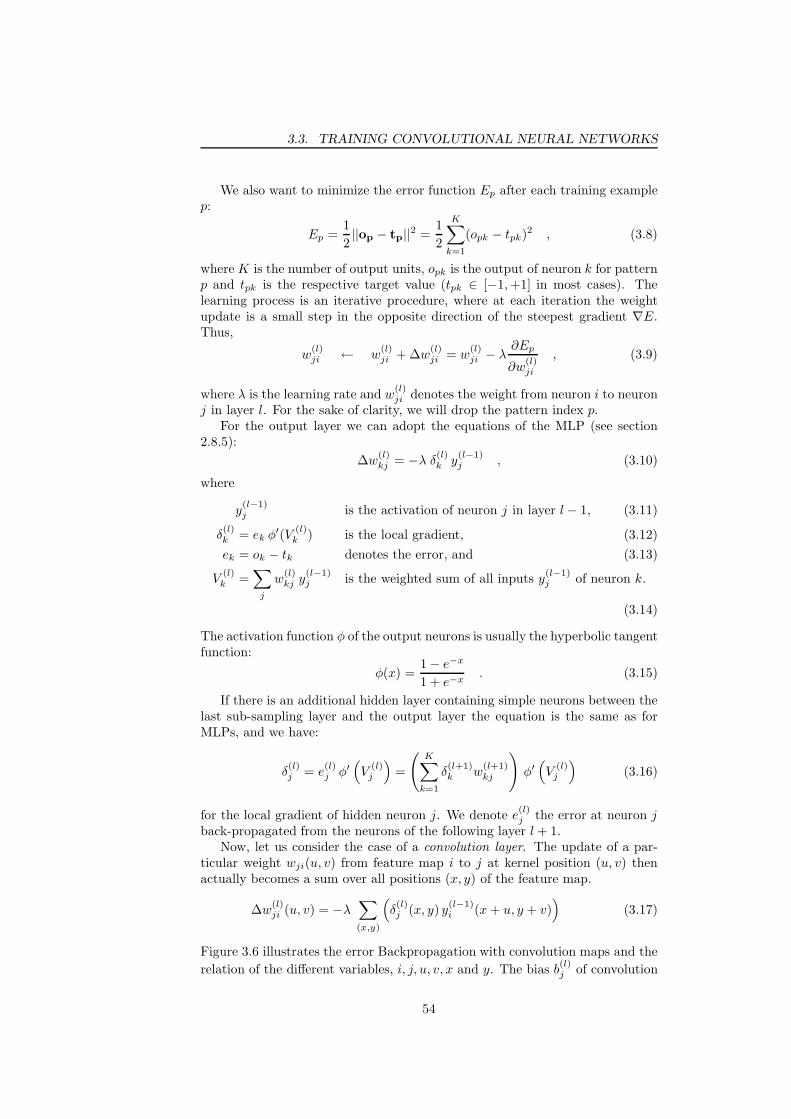
3.3. TRAINING CONVOLUTIONAL NEURAL NETWORKS
We also want to minimize the error function Ep after each training examplep:
Ep =1
2||op − tp||
2 =1
2
K∑
k=1
(opk − tpk)2 , (3.8)
where K is the number of output units, opk is the output of neuron k for patternp and tpk is the respective target value (tpk ∈ [−1, +1] in most cases). Thelearning process is an iterative procedure, where at each iteration the weightupdate is a small step in the opposite direction of the steepest gradient ∇E.Thus,
w(l)ji ← w
(l)ji + ∆w
(l)ji = w
(l)ji − λ
∂Ep
∂w(l)ji
, (3.9)
where λ is the learning rate and w(l)ji denotes the weight from neuron i to neuron
j in layer l. For the sake of clarity, we will drop the pattern index p.For the output layer we can adopt the equations of the MLP (see section
2.8.5):
∆w(l)kj = −λ δ
(l)k y
(l−1)j , (3.10)
where
y(l−1)j is the activation of neuron j in layer l − 1, (3.11)
δ(l)k = ek φ′(V
(l)k ) is the local gradient, (3.12)
ek = ok − tk denotes the error, and (3.13)
V(l)k =
∑
j
w(l)kj y
(l−1)j is the weighted sum of all inputs y
(l−1)j of neuron k.
(3.14)
The activation function φ of the output neurons is usually the hyperbolic tangentfunction:
φ(x) =1− e−x
1 + e−x. (3.15)
If there is an additional hidden layer containing simple neurons between thelast sub-sampling layer and the output layer the equation is the same as forMLPs, and we have:
δ(l)j = e
(l)j φ′
(
V(l)j
)
=
(K∑
k=1
δ(l+1)k w
(l+1)kj
)
φ′(
V(l)j
)
(3.16)
for the local gradient of hidden neuron j. We denote e(l)j the error at neuron j
back-propagated from the neurons of the following layer l + 1.Now, let us consider the case of a convolution layer. The update of a par-
ticular weight wji(u, v) from feature map i to j at kernel position (u, v) thenactually becomes a sum over all positions (x, y) of the feature map.
∆w(l)ji (u, v) = −λ
∑
(x,y)
(
δ(l)j (x, y) y
(l−1)i (x + u, y + v)
)
(3.17)
Figure 3.6 illustrates the error Backpropagation with convolution maps and the
relation of the different variables, i, j, u, v, x and y. The bias b(l)j of convolution
54
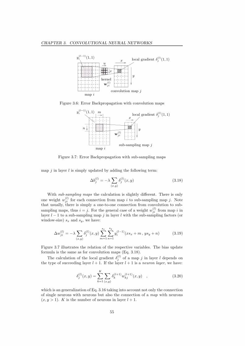
CHAPTER 3. CONVOLUTIONAL NEURAL NETWORKS
y(l−1)i (1, 1)
map iconvolution map j
kernel
w(l)ji
u
v
x
y
local gradient δ(l)j (1, 1)
Figure 3.6: Error Backpropagation with convolution maps
y(l−1)i (1, 1)
map isub-sampling map j
w(l)ji
m
n
x
y
local gradient δ(l)j (1, 1)
Figure 3.7: Error Backpropagation with sub-sampling maps
map j in layer l is simply updated by adding the following term:
∆b(l)j = −λ
∑
(x,y)
δ(l)j (x, y) (3.18)
With sub-sampling maps the calculation is slightly different. There is only
one weight w(l)ji for each connection from map i to sub-sampling map j. Note
that usually, there is simply a one-to-one connection from convolution to sub-
sampling maps, thus i = j. For the general case of a weight w(l)ji from map i in
layer l− 1 to a sub-sampling map j in layer l with the sub-sampling factors (orwindow-size) sx and sy, we have:
∆w(l)ji = −λ
∑
(x,y)
δ(l)j (x, y)
sx∑
m=1
sy∑
n=1
y(l−1)i (xsx + m , ysy + n) (3.19)
Figure 3.7 illustrates the relation of the respective variables. The bias updateformula is the same as for convolution maps (Eq. 3.18).
The calculation of the local gradient δ(l)j of a map j in layer l depends on
the type of succeeding layer l + 1. If the layer l + 1 is a neuron layer, we have:
δ(l)j (x, y) =
K∑
k=1
∑
(x,y)
δ(l+1)k w
(l+1)kj (x, y) , (3.20)
which is an generalization of Eq. 3.16 taking into account not only the connectionof single neurons with neurons but also the connection of a map with neurons(x, y > 1). K is the number of neurons in layer l + 1.
55

3.3. TRAINING CONVOLUTIONAL NEURAL NETWORKS
If the succeeding layer is a convolution layer, we have:
δ(l)j (x, y) =
∑
k∈Kc
∑
(u,v)
δ(l+1)k (x, y) · w
(l+1)kj (u, v) , (3.21)
where Kc denotes the set of maps in layer l + 1 connected to the convolutionmap j in layer l. It has to be taken into account that the convolution maskcannot cross the border of layer l. Thus, the respective terms are not includedin the above sum.
In the case of layer l +1 being a sub-sampling layer, the local gradient is thefollowing:
δ(l)j (x, y) =
∑
k∈Ks
δ(l+1)k (⌊x/sx⌋, ⌊y/sy⌋) · w
(l+1)kj (3.22)
where sx, sy are the sub-sampling factors, Ks denotes the set of maps in layerl+1 connected to the sub-sampling map j in layer l and ⌊·⌋ is the floor function.
Algorithm 8 summarizes the online Backpropagation algorithm for CNNscomposed of several alternating convolution and sub-sampling layers followedby one or more neuron layers.
3.3.2 Other training algorithms proposed in the literature
Although, Error Backpropagation is the most commonly used training algorithmfor CNNs, some alternatives have been proposed in the literature. In principle,most of the learning algorithms for MLPs can be used for CNNs too if onetakes into account weight sharing. However, in practice, the standard onlineBackpropagation algorithms outperforms these methods in most applications.Nevertheless, we will outline here some of the alternatives presented in theliterature and briefly explain how they have been applied to CNNs.
Extending the Neocognitron learning algorithm where each layer is trainedseparately, Neubauer [170] presented a hybrid supervised-unsupervised approachwhere the features to recognize do not have to be defined manually. Here,the parameters of the first hidden layer are trained by randomly extractingimage regions of the size of the receptive field from the training images andthen performing a PCA on these image patches or training a 3-layer auto-encoding NN [208, 45]. The same procedure is repeated for each following hiddenlayer where the training image patches are first propagated until the previouslytrained layer, and then the respective output patches of this layer are used asan input for PCA or auto-encoding. This type of learning algorithm can bepreferable when it is not clear which features should be extracted for a giventask, for example face recognition. After having trained all the hidden layer,the weights of the final neuron layer are determined by a supervised algorithm,e.g. LMS fitting.
Li et al . [142] used an extension of the standard Backpropagation algorithm,called Delta-Bar-Delta algorithm, to train a CNN for text detection in images.It adjusts the learning rate for each weight separately according to the evolutionof respective gradients. Thus, at the beginning all learning rates λi of weightswi are initialized to some small value, and at each iteration they are updated
56

CHAPTER 3. CONVOLUTIONAL NEURAL NETWORKS
Algorithm 8 The online Backpropagation algorithm for Convolutional NeuralNetworks1: Initialize all weights of the CNN to some small random value2: Set the learning rates λ(l) to small positive values3: n = 14: repeat
5: for p = 1 to P do
6: propagate pattern xp through the network7: for k = 1 to K do
8: δ(L)k = (ok − tk)
9: end for
10: for layers l = L− 1 to 1 do
11: for maps j = 1 to J do
12: for all positions (x, y) do
13: if layer l + 1 is a neuron layer then
14: δ(l)j (x, y) =
(∑K
k=1
∑
(x,y) δ(l+1)k w
(l+1)kj (x, y)
)
φ′(V(l)k )
15: else if layer l + 1 is a convolution layer then
16: δ(l)j (x, y) =
(∑
k∈Kc
∑
(u,v) δ(l+1)k (x, y) · w
(l+1)kj (u, v)
)
φ′(V(l)k )
17: else if layer l + 1 is a sub-sampling layer then
18: δ(l)j (x, y) =
(∑
k∈Ksδ(l+1)k (⌊x/sx⌋, ⌊y/sy⌋) · w
(l+1)kj
)
φ′(V(l)k )
19: end if
20: end for
21: end for
22: end for
23: for l = 1 to L do
24: for j = 1 to J do
25: for all weights of map/neuron j do
26: if layer l is a convolution layer then
27: ∆w(l)ji (u, v) = −λ(l)
∑
(x,y)
(
δ(l)j (x, y) y
(l−1)i (x + u, y + v)
)
28: else if layer l is a sub-sampling layer then
29: ∆w(l)ji = −λ(l)
∑
(x,y) δ(l)j (x, y)
∑sx
m=1
∑sy
n=1 y(l−1)i (xsx + m , ysy + n)
30: else if layer l is a neuron layer then
31: ∆w(l)ji = −λ(l) δ
(l)j y
(l−1)i
32: end if
33: update weight: w(l)ji ← w
(l)ji + ∆w
(l)ji
34: end for
35: if layer l is a convolution or sub-sampling layer then
36: ∆b(l)j = −λ(l)
∑
(x,y) δ(l)j (x, y)
37: else
38: bias of neurons is already included in the weight vector39: end if
40: update bias: b(l)j ← b
(l)j + ∆b
(l)j
41: end for
42: end for
43: n = n + 144: end for
45: E = 12
∑Pp=1 ||op − tp||
2
46: until E < ǫ or n > maxiter
57

3.3. TRAINING CONVOLUTIONAL NEURAL NETWORKS
as follows:
λi(n) = λi(n− 1) + u if∂E
∂wi
(n) · δi(n− 1) > 0 (3.23)
λi(n) = λi(n− 1) · d if∂E
∂wi
(n) · δi(n− 1) < 0 (3.24)
λi(n) = λi(n− 1) otherwise , (3.25)
where δi denotes the exponential averaged gradient w.r.t. weight wi:
δi(n) = (1− φ) ·∂E
∂wi
(n) + φ · δi(n− 1) , (3.26)
with φ ∈ [0, 1]. u and d are small positive constants, e.g. u = 0.1 and d = 0.9.The weights are then updated as with the standard Backpropagation algorithm:
wi(n) = wi(n− 1)− λi(n) ·∂E
∂wi
(n) . (3.27)
Li et al . [142] showed that the Delta-Bar-Delta algorithm converges faster thanBackpropagation with fixed learning rates and momentum term. However, theperformance in terms of the detection rate of the CNN trained with the Delta-Bar-Delta algorithm is slightly inferior.
Ouellette et al . [178] proposed a learning method based on Genetic Algo-rithms (GA) and applied it to a CNN used to detect cracks in sewer pipes.Their motivation for using a GA instead of Backpropagation is the commonassumption that GAs are less sensitive to getting stuck in local minima duringthe learning process. The idea of GAs is based on evolutionary concepts, i.e.a certain number of possible solutions, i.e. weight configurations, forming theso-called population is simultaneously maintained. Each solution, called chro-mosome, has to be encoded in a string of symbols, in this case a sequence ofbits representing the integer weight values from 0 to 255 in binary form (from−127 to 128 for biases). Before training starts, the population is initialized withrandom chromosomes. Then, at each iteration, the following steps are repeateduntil a global evaluation criteria is satisfied:
1. Fitness evaluation: The fitness of each member is evaluated, i.e. the per-formance of the CNN on the training set with the respective weight con-figuration.
2. Selection: A subset of members, the parents, with the highest fitness valueis selected to produce the offspring for the next generation.
3. Crossover: The chromosomes of the selected parents are split into two atrandom positions and the resulting partial bit sequences are combined toform the offspring, i.e. the new weight configurations.
4. Mutation and Creep: 1% of the current population is selected for muta-tion and creeping. Mutation means that the respective chromosome israndomly changed within ±1%. Creeping is a similar technique whichscales a chromosome by a random factor between −1 and +1.
Although the authors claim that the proposed algorithm is simpler to im-plement than Backpropagation they could not notice a significant performanceimprovement in terms of accuracy for the given application.
58

CHAPTER 3. CONVOLUTIONAL NEURAL NETWORKS
Figure 3.8: The architecture of LeNet-5
3.4 Extensions and variants
Many variants of the CNN model described in section 3.2.2 exist. Usually,the number of layers, the number of feature maps and their dimensions andthe connection scheme are adapted to the given problem. Unfortunately, theseparameters have to be determined experimentally as, up to the present, thereis no algorithm to automatically determine the optimal architecture of a CNNfor a given classification task. However, besides the architectural variants, therehave been some major enhancements to the CNN model of LeCun et al . [134].In the following, we will present the most important ones.
3.4.1 LeNet-5
A more complex CNN has been presented by LeCun et al . [136] and applied tohandwritten character recognition. The authors called this architecture, LeNet-5. A larger training set has also been used to train this network improvingits overall performance in terms of recognition rate as well as its generalizationcapacity. Figure 3.8 illustrates the principal architecture of LeNet-5.
It is composed of 7 layers, not counting the input layer. The input image is ofsize 32×32 pixels. As with LeNet-1, the first five layers, C1, S2, C3, S4, C5, arealternating convolution and sub-sampling layers with a 5× 5 convolution maskand a sub-sampling factor of 2 respectively. The dimensions of the individualmaps are noted in Fig. 3.8. The connections between the units of the respectivelayers is similar to LeNet-1, i.e. a full connection of the first layer to the inputimage and one-to-one connections in the sub-sampling layers. However, layer C3follows a special non-symmetric connection scheme which is described in table3.1. The convolution maps in C5 have a dimension of only (1, 1) as the size ofthe maps in S4 is 5× 5. Further, they are fully connected to each sub-samplingmap leading to a high number of trainable parameters in this layer (i.e. 48,120).
Layer F6 is an additional hidden neuron layer, fully connected to layer C5and composed of 84 units. The actual novel idea of LeNet-5 lies in the outputlayer which consists of fully connected Radial Basis Function (RBF) units, onefor each character to recognize. To compute the outputs of a RBF unit yi, wehave:
y(6)i =
∑
j
(xj − w(6)ji )2 . (3.28)
Thus, each RBF unit computes the squared Euclidean distance between its 84-
dimensional input vector xj and its weight vector w(6)ji . Further, the weight
59

3.4. EXTENSIONS AND VARIANTS
0 1 2 3 4 5 6 7 8 9 10 11 12 13 14 15
0 X X X X X X X X X X1 X X X X X X X X X X2 X X X X X X X X X X3 X X X X X X X X X X4 X X X X X X X X X X5 X X X X X X X X X X
Table 3.1: The connection scheme of layer C3 of Lenet-5: a cross indicatesa connection between a particular feature map in S2 (row) and a map in C3(column)
vectors of layer F6, i.e. the centers of the RBFs, are fixed at the beginning insuch a way that the 84 values are either −1 or +1 and form a 7 × 12 matrixrepresenting a stylized image of the character. Thus, similar characters, like theuppercase “O”, lowercase “o”, and zero, will produce a similar output. Thismay be helpful for a linguistic post-processor working on the word level whichcould eliminate ambiguities due to confusions of similar characters.
An important point to note is the special error function used by LeCun etal . :
E(W ) =1
P
P∑
p=1
(
y(6)pDp
+ log(e−j +∑
i
e−y(6)pi )
)
, (3.29)
where P is the number of training patterns, y(6)pi is the activation of output
neuron i when presenting pattern p, and Dp is the desired class of pattern p.Minimizing E means minimizing the two terms in the above equation. The first
term, y(6)pDp
, represents the Euclidean distance of the desired output neuron tothe 84-dimensional RBF center. Using only this term could lead to a trivialsolution where all outputs are always zero. Hence, the second term has beenintroduced to also incorporate the outputs of the other neurons, and thereforeit has a discriminative function. It ensures that the RBF centers are kept apartfrom each other and inhibits the trivial case where they “collapse” to the zerosolution. The positive constant j prevents the error function from a furtherincrease for classes that have already large outputs.
3.4.2 Space Displacement Neural Networks
CNNs have a fixed size input layer, also called retina, which can be used todetect or recognize particular objects in images or any other visual structurethey have been trained to process. For example, a CNN trained to recognizehandwritten characters requires the characters presented to the input to be size-normalized and more or less centered. However, there are applications wherethe size of the input is variable, such as the recognition of words or sentences orfor detection tasks, like face detection, where the input images to process canbe of arbitrary size.
A possible solution to this would be to pre-process the variable-size inputimage and segment it into different parts, e.g. the characters of a word or sen-tence. Unfortunately, there does not exist any reliable technique to perform
60

CHAPTER 3. CONVOLUTIONAL NEURAL NETWORKS
Figure 3.9: A Space Displacement Neural Network
this segmentation in most applications because of the too high variability of thepattern to recognize or detect. We therefore would have to place the retina ateach location in the input image and propagate the respective values to obtainthe output of the NN for that particular sub-region of the image. However, attwo neighboring positions, there is a large amount of common computation asthe sub-regions to process overlap and the convolution operations are the samein the overlapping parts. To take advantage of this, we can actually increase thesize of the retina and all the convolution and sub-sampling layers accordingly.Thus, the convolution and sub-sampling with the respective masks is performedon the whole input image. Consequently, the output layer has to be repli-cated over all possible locations, and it effectively becomes a convolution layer.This trick leads to an architecture called Space Displacement Neural Network(SDNN). Figure 3.9 illustrates this by means of a CNN for connected characterrecognition. The output of the SDNN represents a sequence of outputs of therespective simple CNN at each possible location. In order to perform the finalrecognition or detection, this sequence has to be interpreted further in a sepa-rate post-processing step because at neighboring positions of a present objectthe SDNN might give the same answer due to some translation invariance of theCNN. Thus, there has to be some sort of grouping yielding exactly one responsefor each object to detect or recognize. Further, when the object to recognizeis composed of a sequence of adjacent single entities, as the words in charac-ter recognition, the output of the SDNN between two such entities (characters)might be rather arbitrary and has to be discarded.
A classical approach to post-process the output sequence of a SDNN is to usea HMM. Such hybrid solutions have been proposed for example in the contextof handwritten multi-digit or word recognition [121, 156, 19].
3.4.3 Siamese CNNs
Siamese Neural Networks have first been presented by Bromley et al . [29] usingTime Delay Neural Networks (TDNN) and applying them to the problem ofsignature verification, i.e. to verify the authenticity of signatures. This ideawas then adopted by Chopra et al . [39] who used Siamese CNNs and employedthem in the context of face verification. More precisely, the system receives twoface images and has to decide if they belong to the same person or not.
Siamese NNs learn a non-linear similarity metric by repeatedly presentingpairs of positive and negative examples, i.e. pairs of examples belonging to
61

3.4. EXTENSIONS AND VARIANTS
X1 X2
EW
||GW (X1)−GW (X2)||
W
GW (X1) GW (X2)
CNNCNN
Figure 3.10: Illustration of a Siamese Convolutional Neural Network
the same class or not. The principal idea is to train the NN to map the inputvectors into a non-linear subspace such that a simple distance, e.g. the Euclideandistance, in this subspace approximates the “semantic” distance in the inputspace. That means, two images of the same category are supposed to yield asmall distance in this subspace and two images of a different category a largedistance. Let us call this mapping GW (X) and its parameters (i.e. weights) W.Thus, the goal is to learn the parameters W of the function GW (X) such thatthe similarity metric
EW (X1,X2) = ||GW (X1)−GW (X2)|| (3.30)
is small if X1 and X2 belong to the same class and large if they belong todifferent classes. The choice of GW (X) is arbitrary and, in this case, is a CNN.Note that the parameters W, i.e. the weights, are the same for both inputs,hence the name “siamese” NN, and therefore the distance metric is symmetric.Fig. 3.10 illustrates the functional scheme of this learning machine.
To make the system behave in the desired way, we need to define a globalenergy function, or loss function, L(W) such that minimizing it decreases thedistance between examples belonging to the same class (genuine pairs) andincreases the distance between examples belonging to different classes (impostorpairs). A possible energy function would be:
L(W) =P∑
i=1
((1− Y i)LG(EW (X1,X2)i) + Y i LI(EW (X1,X2)i)
), (3.31)
where P is the number of image pairs, (X1,X2)i is the i-th image pair andY i its label, i.e. 1 for a genuine and 0 for an impostor pair. LG and LI arethe energy functions for genuine and impostor pairs respectively, where LG ismonotonically increasing and LI is monotonically decreasing. Chopra et al .[39] require some more conditions to be satisfied, e.g. the existence of a margin,and they formalize some properties of LG and LI in order to ensure a correctbehavior of the siamese CNN. We refer to [39] for more details on this.
The energy function for genuine pairs is usually defined as:
LG = E2W , (3.32)
62

CHAPTER 3. CONVOLUTIONAL NEURAL NETWORKS
0
2
4
6
8
10
12
14
16
18
0 1 2 3 4 5 6 7
LGLI
||GW (X1) − GW (X2)||
Figure 3.11: Example of positive (genuine) and negative (impostor) error func-tions for Siamese CNNs
i.e. we want the distance to be zero for pairs of examples belonging to the samecategory. However, the choice of LI is more difficult. In general, we don’t knowthe exact distance of an impostor pair, e.g. the face images of two differentpersons. A possible solution is to use:
LI = e−tEW (3.33)
with t being a positive constant. This prevents the projected vectors of twodifferent classes from being too close. Chopra et al . [39] used the followingglobal energy function:
L(W) =
P∑
i=1
(
(1 − Y i)2
Q(EW (X1,X2)i)
2+ Y i 2Qe−
2.77Q
EW (X1,X2)i
)
,
(3.34)where the constant Q is the upper bound of EW . Figure 3.11 shows the functionsLG and LI for the one-dimensional case.
The architecture of the CNN in [39] is composed of 6 layers:
• C1: a convolution layer with 15 feature maps and kernel size 7× 7
• S2: a sub-sampling layer containing 15 maps; sub-sampling window size:2× 2
• C3: a convolution layer with 45 feature maps and kernel size 6 × 6; theconnection scheme is similar to the one of LeNet-5 (see table 3.1)
• S4: a sub-sampling layer containing 45 maps; sub-sampling window size:4× 3
• C5: a fully connected convolution layer with 250 feature maps and kernelsize 5× 5
• F6: a fully connected output layer containing 50 neurons.
The input layer of this CNN has the dimension 46× 56.Training is performed using a set of positive and negative examples, i.e.
randomly selected genuine pairs and impostor pairs. At each training iteration,a positive pair and a negative pair is presented to the network. To update
63
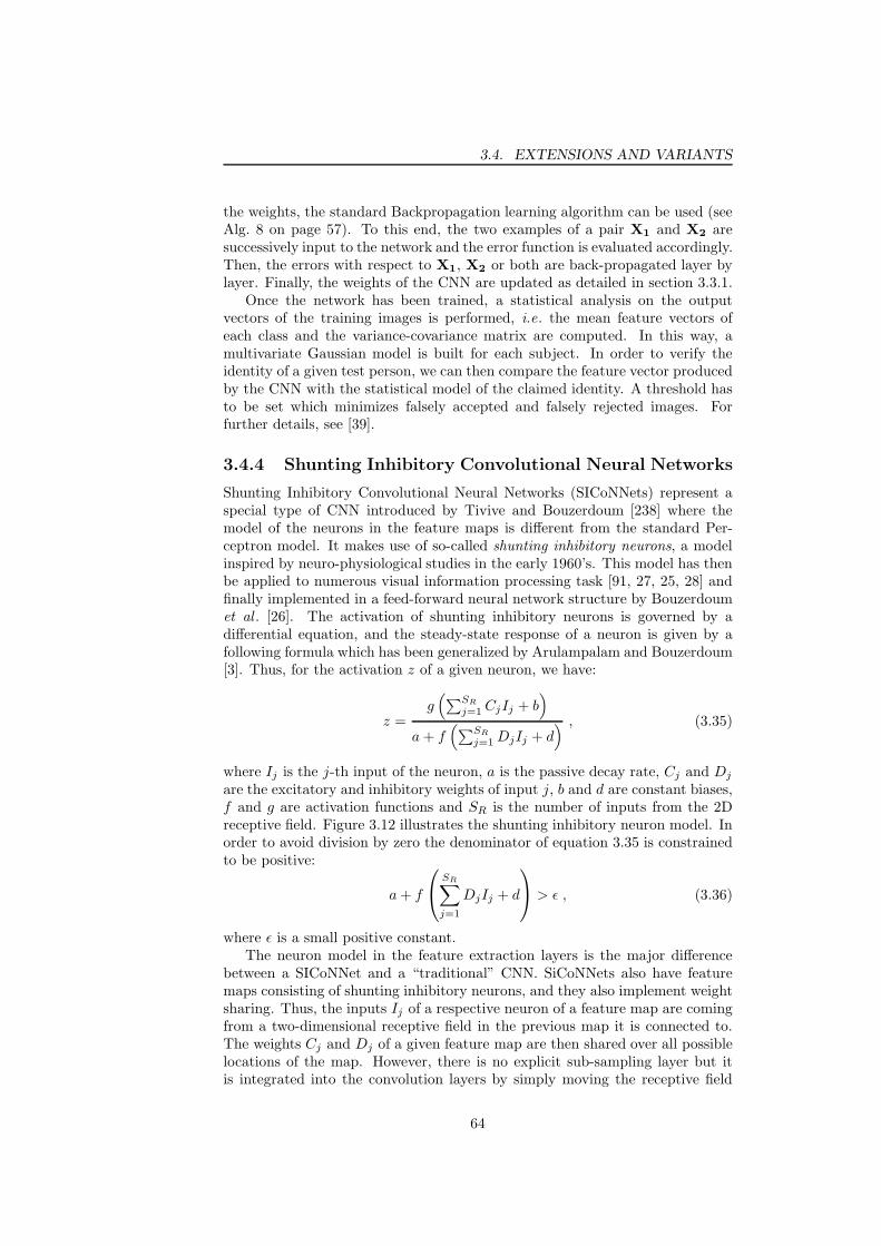
3.4. EXTENSIONS AND VARIANTS
the weights, the standard Backpropagation learning algorithm can be used (seeAlg. 8 on page 57). To this end, the two examples of a pair X1 and X2 aresuccessively input to the network and the error function is evaluated accordingly.Then, the errors with respect to X1, X2 or both are back-propagated layer bylayer. Finally, the weights of the CNN are updated as detailed in section 3.3.1.
Once the network has been trained, a statistical analysis on the outputvectors of the training images is performed, i.e. the mean feature vectors ofeach class and the variance-covariance matrix are computed. In this way, amultivariate Gaussian model is built for each subject. In order to verify theidentity of a given test person, we can then compare the feature vector producedby the CNN with the statistical model of the claimed identity. A threshold hasto be set which minimizes falsely accepted and falsely rejected images. Forfurther details, see [39].
3.4.4 Shunting Inhibitory Convolutional Neural Networks
Shunting Inhibitory Convolutional Neural Networks (SICoNNets) represent aspecial type of CNN introduced by Tivive and Bouzerdoum [238] where themodel of the neurons in the feature maps is different from the standard Per-ceptron model. It makes use of so-called shunting inhibitory neurons, a modelinspired by neuro-physiological studies in the early 1960’s. This model has thenbe applied to numerous visual information processing task [91, 27, 25, 28] andfinally implemented in a feed-forward neural network structure by Bouzerdoumet al . [26]. The activation of shunting inhibitory neurons is governed by adifferential equation, and the steady-state response of a neuron is given by afollowing formula which has been generalized by Arulampalam and Bouzerdoum[3]. Thus, for the activation z of a given neuron, we have:
z =g(∑SR
j=1 CjIj + b)
a + f(∑SR
j=1 DjIj + d) , (3.35)
where Ij is the j-th input of the neuron, a is the passive decay rate, Cj and Dj
are the excitatory and inhibitory weights of input j, b and d are constant biases,f and g are activation functions and SR is the number of inputs from the 2Dreceptive field. Figure 3.12 illustrates the shunting inhibitory neuron model. Inorder to avoid division by zero the denominator of equation 3.35 is constrainedto be positive:
a + f
SR∑
j=1
DjIj + d
> ǫ , (3.36)
where ǫ is a small positive constant.The neuron model in the feature extraction layers is the major difference
between a SICoNNet and a “traditional” CNN. SiCoNNets also have featuremaps consisting of shunting inhibitory neurons, and they also implement weightsharing. Thus, the inputs Ij of a respective neuron of a feature map are comingfrom a two-dimensional receptive field in the previous map it is connected to.The weights Cj and Dj of a given feature map are then shared over all possiblelocations of the map. However, there is no explicit sub-sampling layer but itis integrated into the convolution layers by simply moving the receptive field
64

CHAPTER 3. CONVOLUTIONAL NEURAL NETWORKS
......
Σ
Σ
+
+
+
÷
a
b
d
f()
g()
I1
I1
I2
I2
I3
I3
ISR
ISR
C1
C2
C3
CSR
D1
D2
D3
DSR
z
Figure 3.12: The shunting inhibitory neuron model
by steps of two pixels in each direction. In this way, the dimension of theresulting map is about two times smaller, and convolution and sub-samplinglayers are combined into one layer. Note that here the sub-sampling does notimply an averaging operation (with trainable parameters) like in the CNN modelof LeCun. The bias terms b and d can either be common for each feature mapor one can have a different bias for each position of the respective feature map,i.e. each shunting inhibitory neuron.
The output layer is rather different from the preceding feature extractionlayers. It performs an averaging over 2× 2 non-overlapping sub-regions of thepreceding convolution map. The model of the output neurons is the Perceptron(c.f . section 2.8.2). Thus, the activation of a given neuron is the result of theactivation function applied to the weighted sum of the inputs and the bias. Theoutput neurons are fully connected to the preceding feature maps.
Figure 3.13 shows the architecture of one of the first SICoNNets proposedby Tivive and Bouzerdoum [238] and applied to face detection. It has one inputlayer of size 20× 20, two hidden convolution layers with receptive fields of size5 × 5 and a neuron output layer. The authors compared different connectionschemes for the second convolution layer:
1. fully connected: each feature map is connected to every feature map inthe first convolution layer
2. Toeplitz connected: each feature map of the first convolution layer is con-nected to several maps in the second convolution layer in an overlappingmanner (see Fig. 3.13)
3. binary connected: each feature map of the first convolution layer is con-nected to two feature maps in the second convolution layer. There isno overlapping, i.e. each feature map of the second convolution layer isconnected to only one map of the preceding layer.
For training a SICoNNet, in principal, any training algorithm for feed-
65

3.4. EXTENSIONS AND VARIANTS
input layer
output layer
1st convolution/
2nd convolution/sub-sampling layer
sub-sampling layer
averaging
Figure 3.13: The SICoNNet architecture proposed by Tivive et al . [238]
forward NNs can be used. The trainable parameters of SICoNNets are theexcitatory and inhibitory weights Cj and Dj for each receptive field and thebiases b and d as well as the passive decay rate a for each neuron (or each fea-ture map). In [238] the RPROP algorithm (c.f . Alg. 5) has been employed fortraining the face detection SICoNNet. To this end, a classical error function Ehas been defined:
E =1
2(y − t)2 , (3.37)
where y is the output of the NN and t is the target output for one particularpattern. Then, the gradient of E w.r.t. each trainable parameter is calculatedin order to perform Error Backpropagation as described for MLPs in section2.8.5.
In a later work Tivive and Bouzerdoom [239] implemented 16 different train-ing methods and compared them in terms of classification rates and convergencespeed on a face/non-face classification problem. They also propose two new hy-brid training algorithms. The first is based on RPROP, QuickPROP and Super-SAB and is called QRPROP. The second integrates an additional Least Squares(LS) optimization for the final layer and is called QRPROPLS. The performanceof these algorithms was tested on three different architectures with differentconnections schemes: fully connected, Toeplitz connected and binary connectedas described above. The experimental results show that Toeplitz connectedand binary connected networks slightly outperform fully connected architec-tures. Good classification rates were obtained with modified Broyden-Fletcher-Goldfarb-Shanno (BFGS) methods, variants of the Levenberg-Marquardt opti-mization technique and the QRPROPLS method proposed by the authors. Interms of convergence speed, the best results were obtained with QRPROPLSand a hybrid Levenberg-Marquardt/LS algorithm. For details of the trainingalgorithms refer to [239].
66

CHAPTER 3. CONVOLUTIONAL NEURAL NETWORKS
layer l+1
layer l
Figure 3.14: The connection scheme of the SCNN proposed by Gepperth. Solidellipses represent receptive fields. Dotted ellipses represent cells. The dashedlines are receptive field connections where equal line colors stand for sharedweights. Here the overlap is one pixel/neuron.
3.4.5 Sparse Convolutional Neural Networks
The idea of Sparse Convolutional Neural Networks (SCNN) is to reduce as muchas possible the redundancy in the feature extraction layers. That means differ-ent feature extractors (e.g. convolution filters) should be as “independent” aspossible and the information they extract should be non-redundant, i.e. sparse,and in a way complementary.
Gepperth [85] proposed a SCNN which achieves sparsity with a special typeof connectivity and an orthogonalization of the convolution masks. The archi-tecture he presented does not use sub-sampling layers, but a sub-sampling effectis obtained by reducing the overlap of the receptive fields in the convolution lay-ers. Figure 3.4.5 illustrates the connection scheme for the one-dimensional case.Here, instead of putting the result of each convolution into a separate featuremap (as in LeCun’s model) the outputs of all filters (i.e. the weighted sum withthe convolution masks) at one particular image location are grouped into a so-called cell leading to only one feature map in each layer containing a certainnumber of cells, one for each receptive field location in the preceding layer. Asigmoidal activation function φ(x) = x
1+|x| and a trainable bias has been used
for each neuron.In order to reduce the redundancy in the convolution filters, the filter pa-
rameters in each cell are orthogonalized after every training epoch. To thisend, a matrix W is formed where each column represents the parameters (i.e.weights) of one particular convolution mask. The orthogonalization of W isthen performed in an iterative manner (see [107] for details):
W0 = W/||W|| (3.38)
Wt+1 = 1.5Wt − 0.5WtWTt Wt . (3.39)
In the work presented by Gepperth [85], the error function to minimize is theclassical mean squared error of the network outputs w.r.t. the desired outputs.The author experimented with different numbers of layers and varying overlaps.The final layer contained a single neuron and the SCNN has been trained for avisual classification task.
Ranzato et al . [193] also proposed a CNN-based approach which learns inan unsupervised manner sparse and also shift-invariant feature extractors. Theauthors proposed an encoder-decoder framework and applied it to object recog-nition. The encoder uses a specific type of CNN with alternating convolutionand max-pooling layers where each pair of layers is trained separately. A max-pooling layer is a sub-sampling layer where each map is connected to a convolu-
67

3.4. EXTENSIONS AND VARIANTS
0
1
0
1
encoder decoder
convolution max−poolinginput upsampling reconstruction outputlayerlayer layerlayer
sparsecode Z
Figure 3.15: The sparse, shift-invariant CNN model proposed by Ranzato et al .
tion map in the preceding layer, and each unit in a max-pooling map computesthe maximum value within a small neighborhood in the respective convolutionmap. Figure 3.15 illustrates this architecture with only one convolution andmax-pooling layer. To achieve shift-invariance, the transformation parametersU are retained at the output of the encoder and used to reconstruct the inputimage in the decoder from the shift-invariant representation Z.
Learning was performed in an EM-like fashion alternating the minimizationof the optimal code Z∗ w.r.t. a global energy function and the minimization ofthe weight parameters of the encoder and decoder, WC and WD, w.r.t. thedesired output image Y and the optimal code Z∗ respectively (see [193] fordetails).
In order to have the encoder produce sparse codes, an additional non-linearlogistic function has been used between the encoder and the decoder. Thisfunction transforms zi(k), i.e. the i-th component of the k-th training exampleinto a sparse code zi(k):
zi(k) =eβzi(k)
ζi(k), with ζi(k) = eβzi(k) +
1− η
ηζi(k − 1) , (3.40)
where η ∈ [0, 1] controls the sparseness of the code and β > 0 determines thegain of the logistic function. In a way, this function memorizes the history ofthe activation of a unit, and it can produce a large value close to 1 only if theunit has undergone a long enough quiescent period.
Ranzato et al . [193] also extended the simple encoder to a hierarchical two-level feature extractor by using an additional convolution and a max-poolinglayer trained separately on the sparse features extracted at the first level. Inthis way, more complex features can be extracted in an unsupervised way.
68
CHAPTER 3. CONVOLUTIONAL NEURAL NETWORKS
3.5 Some Applications
CNNs have been employed in numerous visual pattern recognition systems fromdifferent contexts. To give a short overview, we will list here some of the appli-cation published in the literature.
As mentioned in the beginning of this chapter, Fukushima was the first toapply a CNN, the so-called Neocognitron, to the problem of handwritten digitrecognition [74] and later to handwritten isolated character recognition [78]. Amore complex CNN architecture has then been used by Fukushima and Wake[77] to segment and recognize handwritten connected characters.
LeCun et al . [134] also proposed a CNN for handwritten digit recognition,the so-called LeNet-1 (see section 3.2.2). A later version, the LeNet-5 (seesection 3.4.1) [136], has been designed to also recognize letters and special char-acters, and the authors further propose an integration into a graph frameworkrecognizing the handwritten amounts on bank checks. Neubauer [170] applieda Neocognitron and a modified version to the problem of handwritten digitrecognition and compared the results with those of an MLP a SOM and anauto-associative NN. He also conducted experiments on a face recognition task.Recently, Saidane and Garcia [211] applied CNNs to the problem of scene textrecognition where the characters to recognize usually show considerable vari-ations in shape, color and background. In another work [212] they furtherpropose a robust method for text binarization employing a specific CNN archi-tecture that is trained to directly output the binarized image of the raw inputtext image.
Face analysis is another problem that many researchers tackled with CNN-based approaches. Lawrence et al . [132] for example use a SOM for dimension-ality reduction and then apply a CNN for classification. Further, Fasel [65, 64]uses a CNN architecture with receptive fields of different sizes and applied itto face and facial expression recognition and a combination of both. Osadchyet al . [175] presented a combined face detector and pose estimator based ona CNN architecture. And Matsugu et al . [157, 158] presented a CNN variantwith a spiking neuron model and apply it to face detection and facial expressionrecognition. The face analysis systems presented by Tivive and Bouzerdoum useshunting inhibitory CNNs (SICoNNets). They applied different architectures toface detection [238] and also eye detection [240]. Finally, Chopra et al . [39]proposed a siamese CNN for a face verification problem (see section 3.4.3).
Many other works used CNNs for visual object detection applications invery different contexts. For example, text detection [142], logo detection inTV programs [55], hand detection and tracking [173], lung nodule detection inradiographs [147] or crack detection in sewer pipes [178].
Moreover, LeCun et al . [135] introduced a CNN-based system for view-inva-riant object recognition, e.g. planes or cars, on cluttered background. Finally, anoriginal application of CNNs has been presented by LeCun et al . [137], namelya camera-based steering system for an autonomous mobile robot avoiding ob-stacles in an off-road environment.
The large number of applications in which CNNs have been successfullyemployed illustrates the flexibility and performance of this approach especiallyin visual pattern recognition problems.
69

3.6. CONCLUSION
3.6 Conclusion
In this chapter, we presented a feature extraction and classification technique,called Convolutional Neural Network, which is based on a specific type of NeuralNetwork, the Neocognitron, introduced by Fukushima [74]. The characteristicsof CNNs are receptive fields that extract local features and the concept of “sim-ple” and “complex” cells which, in a hierarchical layer-wise connection scheme,can be used to construct complex, non-linear feature extractors. Further, theprinciple of weight sharing drastically reduces the number of free parameters inthe CNN and therefore improves convergence, reduces computation time andincreases its generalization capacity. The use of sub-sampling can further im-prove the performance of CNNs making the feature extractors invariant to smallshifts and distortions.
An important breakthrough concerning the technique of CNNs has beenachieved when LeCun et al . [134] presented their CNN architecture and trainedit with the Backpropagation algorithm. Following this approach, the features toextract are not chosen “manually” but learned automatically by the algorithmminimizing a given global error function. A further advantage with this modelis that the CNN has not to be trained layer-by-layer but all the parameters areupdated at each training iteration allowing an online application, which can beimportant when not all of the training data is available at the beginning.
We also presented some extensions and variants of CNNs and briefly describehow they are trained and applied in different contexts. In a trade-off betweensimplicity and performance, we chose to adopt and modify the CNN modelof LeCun et al . [134] for all the face analysis applications in this work. To-gether with the online Backpropagation training algorithm, it represents a verypowerful machine learning technique being able to learn very complex non-linearfeature extractors and classifier which can be applied to almost any visual detec-tion and recognition problem. Moreover, the automatic construction of featureextractors and the simultaneous learning of a classifier are clearly an advantageof this technique when applied to face analysis tasks. Obviously, it is ratherdifficult to “manually” determine which visual features are important in faceimages as the faces’ appearance varies considerably under different conditions.
In the following chapter, we will focus on the problem of face detectionin images and different normalization methods in terms of illumination, poseand global alignment. The localization and normalization steps are crucial forfurther processing of face images, notably for face recognition because the per-formance of state-of-the-art face recognition systems depends heavily on theprecision of these preceding steps.
70

Chapter 4
Face detection and
normalization
4.1 Introduction
Face detection or face localization denotes the problem of finding one or severalsub-regions in images, each subregion containing a face, i.e. determining theposition and scale of the respective face regions and sometimes also their rotationangle in the image plane. Face detection algorithms mostly represent theirresults as bounding boxes covering the regions of the image which are supposedto contain faces, i.e. one bounding box per face. Note that most of the faceanalysis tasks, e.g. face recognition, facial expression recognition, facial featuredetection, require the localization of the face as an initial step.
Face detection can imply a pre-processing step conditioning the input imageand performing a kind of normalization, e.g. converting the image to gray-scale,equalizing the intensity histogram of the image or image regions. Usually, thispre-processing is considered to be part of the face detection algorithm.
Additionally, there can be a post-processing step further normalizing theresult of the face detection procedure, e.g. the bounding boxes. Possible opera-tions are illumination normalization, pose normalization or estimation, or facealignment, that means the global alignment of the bounding boxes w.r.t. the faceimages they cover. We will explain these procedures in more detail in sections4.3-4.5, and in the following we will refer to them as face normalization. Facenormalization is an important step in many face analysis applications becauseit eliminates visual information irrelevant to the respective task. For example,in face recognition, varying illumination conditions can cause face images of thesame person to appear considerably different while the face images of two dif-ferent persons under the same illumination conditions might look very similar.Thus, without a preceding illumination normalization the overall classificationmight be rather difficult.
In the following sections, we will first outline the state-of-the-art in facedetection and describe in more detail one method based on CNNs that hasbeen used throughout this work, the Convolutional Face Finder [81]. Then,we will present a brief overview of current illumination normalization and poseestimation techniques, and finally we will focus on the process of face alignment
71

4.2. FACE DETECTION
and present a novel system for global affine alignment of face images usingCNNs.
4.2 Face detection
4.2.1 Introduction
In this section we will first give an overview of current face detection techniquespresented in the literature and then describe one approach in more detail: theConvolutional Face Finder proposed by Garcia and Delakis [81]. This systemis based on CNNs and outperforms other state-on-the-art face detection meth-ods. Face detection algorithms are mostly compared in terms of their detectionrate (i.e. number of correctly detected faces) vs. their false alarm rate (i.e.number of non-face regions erroneously detected as faces) measured on publicface databases, for example the CMU face database [206]. Clearly, one seeks amethod that maximizes the detection rate while minimizing the false alarm rate.Usually, the latter is a rather difficult task as the subset of non-face images ofa given size is considerably larger and more complex than the subset of imagesrepresenting faces.
4.2.2 State-of-the-art
Many approaches to face detection have been proposed in the literature. Hjelmaset al . [98] and Yang et al . [266] presented surveys on the most important of them.They can be roughly divided into two categories: template-based and feature-based methods. In template-based approaches, the input image is scanned ateach possible location by extracting a subregion of varying scale from it andclassifying it as face or non-face.
Sung and Poggio [231] presented such an approach using Neural Networks.They first modeled the distribution of face and non-face images (of size 19× 19pixels) using a clustering algorithm and then calculate for every training examplethe distance to each cluster center forming 24 element feature vectors. Then,they trained a Neural Network with these feature vectors to distinguish betweenfaces and non-faces. Osuna et al . [176] proposed a similar approach but usingSupport Vector Machines (SVM) instead of a Neural Network.
Colmenarez and Huang [40] proposed a system based on Kullback rela-tive information (Kullback divergence) to measure the difference between joint-histograms computed for each pair of pixels in the face images of the trainingset, for the classes of faces and non-faces. With the two trained probability mod-els one is then able to localize faces by scanning the input image at differentscales and determining the sub-regions where a pre-defined likelihood measureis above a certain threshold.
Rowley et al . [207] used a Neural Network architecture with a specific con-nection of the hidden layer and applied it directly on the pixels of 20 × 20sub-windows to be classified as face or non-face. In order to reduce the numberof false alarms they trained several Neural Networks and used an arbitrationstrategy for the final classification. Further, they accelerated their face detec-tion system by a two-stage approach using a simple Neural Network to filter
72

CHAPTER 4. FACE DETECTION AND NORMALIZATION
out possible face candidates in the first stage and refine the classification in thesecond stage.
Roth et al . [202] proposed a face detector based on a learning architec-ture called SNoW (Sparse Network of Winnows), which consists of two linearthreshold units, representing the classes of faces and non-faces, that operate onan input space of Boolean features. Features like intensity mean, intensity andvariance were first extracted from a series of sub-windows from the face windowand then discretized into a predefined number of classes to give boolean featuresin a 135,424-dimensional feature space. The system was trained with a simplelearning rule, which increases and decreases weights in cases of misclassification,in order to classify face and non-face boolean features.
Schneiderman and Kanade [218] presented a face detection method basedon a locally sampled three-level wavelet decomposition. Several sets of waveletcoefficients were extracted from chosen sub-bands of the wavelet tree. Thecoefficients were re-quantized to three levels and probabilistic density functionswere built using histograms. Then, they applied Bayes’ rule for the classificationbetween face and non-face patterns.
Heisele et al . [97] proposed an approach based on a Support Vector Machine.They trained the SVM to classify the whole input pattern as face or non-faceusing a set of training images of size 19×19 pixels. The features they extractedare the histogram-normalized image, gradients computed by a Sobel filter andthe outputs of the convolution with some specific Haar wavelets filters. Then,they compared this method with a feature detection-based approach (see section5.2).
Froba and Kullbeck [72] described a detection algorithm calculating orien-tation maps of the input image at different scales. The resulting maps werescanned using an orientation map template of the face.
An efficient method called “Boosted Cascade Detector” has been proposedby Viola and Jones [250]. They made use of simple classifiers summing pixelvalues from adjacent regions of the candidate image patch. Then they combinedmany of these weak classifiers and weighted them in a certain way to finallyobtain a strong classifier being able to distinguish the patch between face ornon-face. The selection and weighting of these weak classifiers was performedby the “Adaboost” algorithm, explained in more detail in section 2.5.
S. Li et al . [143] extended the idea of Viola and Jones and proposed a multi-view face detection method. They applied different levels of detectors, moreor less specialized to specific poses. In a coarse-to-fine approach, the range ofdetectable poses is more and more restricted. If all detectors at a particularlevel fail the candidate region is rejected.
Other techniques are based on standard multivariate statistical analysis.Yang et al . [265], for example, presented two methods which seek to representthe manifold of human faces as a set of subclasses. In the first method, a mix-ture of factor analyzers was used to perform clustering and local dimensionalityreduction within each obtained cluster. The second method uses Kohonen’s self-organizing maps for clustering, Fisher’s linear discriminant to find an optimalprojection for pattern classification and a Gaussian distribution to model theclass-conditional density function of the projected samples for each class. Max-imum likelihood estimates were used for the parameters of the class-conditionaldensity functions and the decision rule.
Feraud et al . [67] proposed a Neural Network approach, based on constrained
73

4.2. FACE DETECTION
generative models (CGM), which are auto-associative fully connected MLPswith three large layers of weights, trained to perform a nonlinear dimension-ality reduction similar to PCA. Classification is obtained by considering thereconstruction errors of the CGMs. The best results were reported using a com-bination of CGMs via a conditional mixture and an MLP filtering out unlikelycandidates. As the computational cost of this method is high, some pre-filteringoperations are required, such as skin color and motion segmentation. Like in theprevious neural based approaches, every tested sub-window was preprocessedusing the approach of Sung and Poggio [231].
More recently, Garcia and Delakis [81] presented a face detection methodusing Convolutional Neural Networks (CNN). Here, specialized filters and clas-sifiers were automatically and conjointly learned by the Neural Network usingface and non-face examples and a specific bootstrapping algorithm. Being par-ticularly robust w.r.t. noise and partial occlusions and producing very few falsealarms, this technique, so far, shows the best performance on difficult public facedatabases such as the CMU database [206]. In section 4.2.3 we will describe thismethod in more detail.
Finally, Osadchy et al . [175] also presented a face detection system based onCNNs. They employed an network architecture similar to LeNet-5 (see section3.4.1) and trained it to map face images with known head pose onto pointsin a low-dimensional manifold parameterized by pose and non-face image ontopoints far away from that manifold. Once the CNN has been trained, it canclassify image sub-regions as face or non-face by applying the mapping to themand calculating the distance between the projected vector and the analyticalmanifold. The advantage of this method is that it performs an implicit poseestimation at the same time as face localization. Additionally, an synergisticeffect of the integration of both has been shown. Another advantage is therelatively large range of pose handled by the system, i.e. [−90, +90] degreesof left/right rotation (yaw) and [-45,+45] degrees of up/down rotation (roll).However, the performance of the method in terms of detection rate and falsealarm rate measured on the CMU data set is inferior to the system proposed byGarcia et al . [81].
Table 4.1 summarizes the performance in terms of detection rate of someof the previously mentioned methods. It can be observed that the methodby Garcia and Delakis compares favorably with the others, especially for lownumbers of false alarms. This shows that this approach separates the face andnon-face spaces in a robust and balanced way. For larger number of false alarms,its results are equivalent to the ones reported for the other methods. It suggeststhat all these detectors reach very similar maximal detection limits.
The previously listed methods are all template-based approaches as they tryto match a global face model onto sub-regions of the image to process. Featurebased approaches [141, 42, 268, 116, 83, 94], however, search for particular facialfeatures in the input image and, most often, reduce the number of candidatesby probabilistic models of feature constellations. The detection of single fea-tures can make these methods more robust to out-of-plane rotation, or partialocclusions of the face. However, in contrast to template-based methods, theyare unsuitable for the detection of low-resolution faces, e.g. 20 × 20 pixels. Inchapter 5, we will outline some facial feature detection methods that have beenemployed for face detection.
Unfortunately, most of the feature-based face detection approaches proposed
74

CHAPTER 4. FACE DETECTION AND NORMALIZATION
Table 4.1: Detection rate vs. false alarm rate of selected face detection methodson the CMU test set.
False alarms
Face detector 0 10 31 65 167
Rowley et al . [207] - 83.2% 86.0% - 90.1%Schneiderman et al . [218] - - - 94.4%Li et al . [143] - 83.6% 90.2% - -Viola and Jones [250] - 76.1% 88.4% 92.0% 93.9%Osadchy et al . [175] - - - 83.0% 88.0%Garcia et al . [81] 88.8% 90.5% 91.5% 92.3% 93.1%
in the literature use different evaluation methods and/or databases which makestheir comparison in terms of performance and precision impossible.
In the following section, we will describe in more detail the ConvolutionalFace Finder (CFF) presented by Garcia and Delakis [81] because it achieves goodperformance in terms of detection rate and because it is based on ConvolutionalNeural Networks.
4.2.3 Convolutional Face Finder
Introduction
The CNN-based face detection system proposed by Garcia and Delakis [81]and dubbed Convolutional Face Finder (CFF) can be classified as a templatematching technique as it verifies the presence or absence of a face at each possiblelocation in the face image employing a sliding-window approach. The CFF hasbeen proven to be one of the best performing face detection methods up to thepresent regarding its high detection rate and low false alarm rate on difficultreal-world images. Therefore, we will use this system throughout the rest of thiswork and further improve it by an additional face alignment system explainedin section 4.5.
Architecture
The architecture of the CFF is essentially a CNN with 7 layers including theinput layer. It is based on the CNN model of LeCun et al . [134] but has adifferent number of feature maps and neurons and notably a different connectionscheme between the layers. Figure 4.1 shows the basic architecture of the CFF.There are two alternating convolutional and sub-sampling layers C1, S1 and C2,S2 followed by two neuron layers N1 and N2. The size of the input layer, i.e.the retina, is 32× 36 pixels.
Layer C1 is composed of four feature maps of size 28× 32 pixels. Each unitin each feature map is connected to a 5× 5 neighborhood into the input retinaof size 32× 36. Each feature map unit computes a weighted sum of its input by25 (5×5) trainable coefficients, i.e. the convolution kernel, and adds a trainable
75
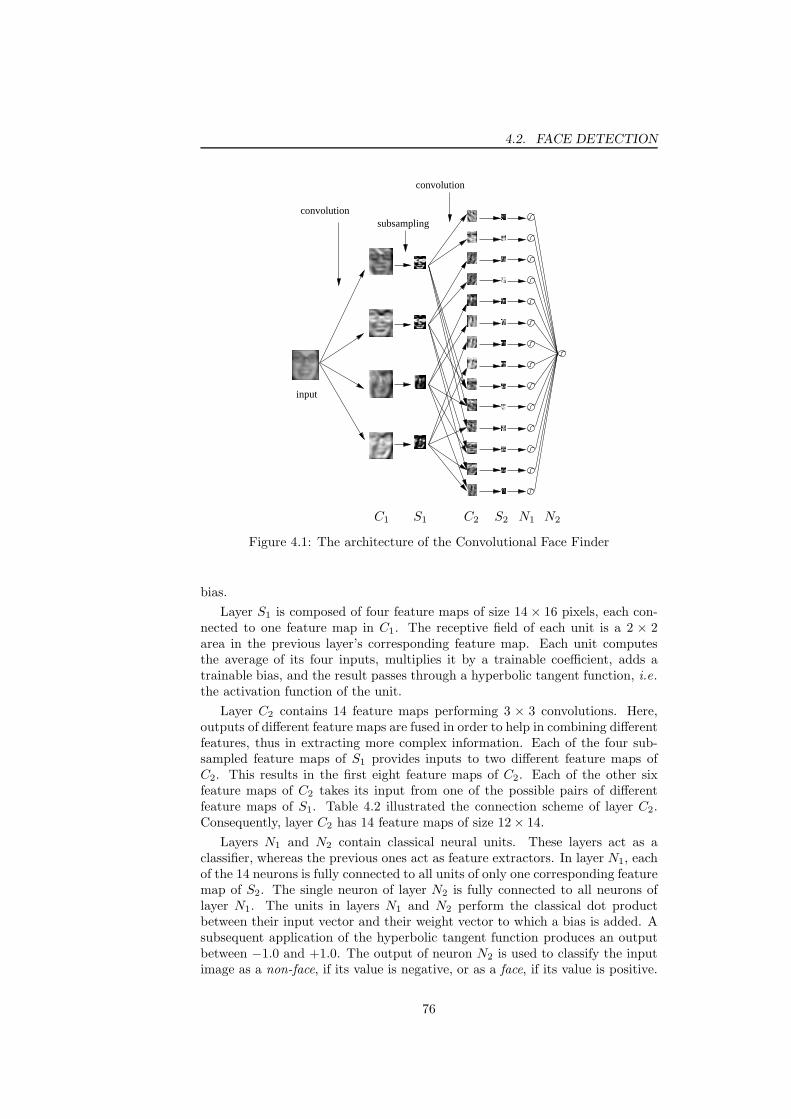
4.2. FACE DETECTION
convolution
convolution
subsampling
input
C1 C2S1 S2 N1 N2
Figure 4.1: The architecture of the Convolutional Face Finder
bias.
Layer S1 is composed of four feature maps of size 14 × 16 pixels, each con-nected to one feature map in C1. The receptive field of each unit is a 2 × 2area in the previous layer’s corresponding feature map. Each unit computesthe average of its four inputs, multiplies it by a trainable coefficient, adds atrainable bias, and the result passes through a hyperbolic tangent function, i.e.the activation function of the unit.
Layer C2 contains 14 feature maps performing 3 × 3 convolutions. Here,outputs of different feature maps are fused in order to help in combining differentfeatures, thus in extracting more complex information. Each of the four sub-sampled feature maps of S1 provides inputs to two different feature maps ofC2. This results in the first eight feature maps of C2. Each of the other sixfeature maps of C2 takes its input from one of the possible pairs of differentfeature maps of S1. Table 4.2 illustrated the connection scheme of layer C2.Consequently, layer C2 has 14 feature maps of size 12× 14.
Layers N1 and N2 contain classical neural units. These layers act as aclassifier, whereas the previous ones act as feature extractors. In layer N1, eachof the 14 neurons is fully connected to all units of only one corresponding featuremap of S2. The single neuron of layer N2 is fully connected to all neurons oflayer N1. The units in layers N1 and N2 perform the classical dot productbetween their input vector and their weight vector to which a bias is added. Asubsequent application of the hyperbolic tangent function produces an outputbetween −1.0 and +1.0. The output of neuron N2 is used to classify the inputimage as a non-face, if its value is negative, or as a face, if its value is positive.
76

CHAPTER 4. FACE DETECTION AND NORMALIZATION
0 1 2 3 4 5 6 7 8 9 10 11 12 13
0 X X X X X1 X X X X X2 X X X X X3 X X X X X
Table 4.2: The connection scheme of layer C2 of the Convolutional Face Finder:a cross indicates a connection between a particular feature map in S1 (row) anda convolution map in C2 (column)
Figure 4.2: Some patterns used for training. The first three rows show somehighly variable face patterns. The last row contains some examples of non-facepatterns produced by the bootstrapping procedure (Courtesy of C. Garcia).
Training
In order to train the CNN, the authors used a set of about 3,700 manuallycropped, highly variable face images extracted from various sources of the In-ternet and from scanned newspapers. The collected images are chosen to effec-tively capture the variability and the richness of natural data in order to trainthe system for operating in uncontrolled environments. No intensity normal-ization such as histogram equalization is performed on the cropped faces. Inorder to create more examples and to enhance the tolerance to small in-planerotations and variations in intensity, a series of transformations are applied tothe initial set of face examples, e.g. small rotations, mirroring and smoothing.The set of initial negative (i.e. non-face) examples is built by randomly croppingregions out of images that do not contain any faces. Then, this set is gradu-ally augmented by a so-called bootstrapping procedure which, every 60 trainingiterations, applies the Neural Network on scenery images not containing anyface and collects the false alarms that give a response above a certain threshold.This threshold is decreased at each step. Thus, the frontier between positiveand negative examples is gradually refined. Figure 4.2 shows some exampleimages of faces and non-faces used for training. The training algorithm is thestandard online Backpropagation with momentum which was slightly adaptedto cope with weight sharing (c.f . Alg. 8 on page 57). For further details on thetraining procedure refer to [81].
The face localization procedure
Figure 4.3 depicts the different steps of face localization with the CFF in agray-scale image containing three faces. In order to detect faces of different
77

4.2. FACE DETECTION
Figure 4.3: The face localization procedure. (1) creation of a multi-scale pyra-mid from the original image. (2) convolution of each image of the pyramid bythe CFF. (3) projection of face candidates to the original scale and fusion ofoverlapping face candidates. (4) application of the CFF in a fine pyramid cen-tered at each face candidate position. (5) classification of each face candidateaccording to the volume of positive answers in the corresponding fine pyramid(Courtesy of C. Garcia).
sizes, the input image is repeatedly sub-sampled by a factor of 1.2, resulting ina pyramid of images (step 1). Each image of the pyramid is then entirely filteredby the CFF (step 2). In fact, this corresponds to a Space Displacement NeuralNetwork (SDNN) applied at several scales (see section 3.4.2). For each imageof the pyramid an image containing the network results is obtained. Because ofthe successive convolutions and sub-sampling operations, this image is approx-imately four times smaller than the original one. This fast procedure may beseen as corresponding to the application of the network retina at every locationof the input image with a step of four pixels in both axis directions, withoutcomputational redundancy.
After processing by this detection pipeline, face candidates (pixels with pos-itive values in the result image) in each scale are mapped back to the inputimage scale (step 3). They are then grouped according to their proximity inimage and scale spaces. Each group of face candidates is fused in a represen-tative face whose center and size are computed as the centroids of the centersand sizes of the grouped faces, weighted by their individual network responses.After applying this grouping algorithm, the set of remaining representative facecandidates serve as a basis for the next stage of the algorithm performing fineface localization and, eventually, false alarm dismissal.
That means, a local search procedure is performed in an area around eachface candidate center in image scale-space (step 4). A reduced search spacecentered at the face candidate position is defined in image scale-space for preciselocalization of the face candidate. It corresponds to a small pyramid centered
78
CHAPTER 4. FACE DETECTION AND NORMALIZATION
at the face candidate center position covering ten equally distant scales varyingfrom 0.8 to 1.5 times the scale of the face candidate. For every scale, thepresence of a face is evaluated on a rescaled grid of 16x16 pixels around thecorresponding face candidate center position. In order to discriminate truefaces from false alarms, the authors took into account both number and valuesof positive answers. Therefore, they considered the volume of positive answers(the sum of positive answer values) in the local pyramid in order to take theclassification decision. Based on the experiments described in the followingsection, a face candidate is classified as face if its corresponding volume is greaterthan a given threshold ThrV ol (step 5). The bottom-right image of Fig. 4.3shows the positions and sizes of the faces detected after local search. One cannotice that the false alarm (up right in the image), previously detected in step4, with a low volume after local search, has been removed using the volumethreshold criterion.
Experimental results
The authors evaluated their method on three different test sets: the first oneis the CMU test set [207] consisting of 130 images and containing 23 images ofthe MIT test set [231]. CMU-125 and MIT-20 are subsets of CMU and MITrespectively, excluding hand-drawn and cartoon faces. The second set is calledWeb test set and contains 215 images randomly chosen from submissions toan interactive online demonstration of the face detection system. Finally, thethird test set is referred to as Cinema and consists of 162 images extracted fromvarious movies and showing faces under very difficult conditions.
Only a few papers, including [265], address the definition of what is a cor-rectly detected face [98]. In the experiments in [81], a detected face is consideredvalid if the face window is not 20% bigger that the real face area and containsboth eyes and mouth. In some papers, reported results of selected methods onthe face databases are difficult to interpret. For a given approach, some resultscorrespond to the maximal detection rate with a high number of false alarmsand others to a lower detection rate with a smaller number of false alarms.Indeed, most face detectors can adjust parameters (usually a threshold) influ-encing detection and false alarm rates. The detection rate is the ratio betweenthe number of successful detections and the number of labeled faces in the testset. The false alarm rate is the ratio between the number of false positive detec-tion and the number of scanned windows. This can be illustrated in terms of aReceiver Operator Characteristic (ROC) curve to show the detection rate versusthe false alarm rate for various values of the threshold. Figure 4.4 depicts theROC curves for the CMU, the Web and the Cinema test sets. Each point on acurve corresponds to a given threshold ThrV ol applied to the volume of positiveanswers in order to classify an image area into face or non-face. Note that quitehigh detection rates were obtained with zero false alarms, i.e. 88.8%, 90.5%and 80.4% for the CMU, the Web and the Cinema test sets respectively. Onthe other hand, the maximum detection rates are 93.3% with 197 false alarms,98.0% with 108 false alarms and 95.3% with 104 false alarms, for the CMU, theWeb and the Cinema test sets respectively. These results are summarized inTable 4.1 on page 75.
Table 4.3 lists the detection rates for various numbers of false detectionsfor the CFF (with ThrV ol = 17.0) as well as for other published systems as
79

4.2. FACE DETECTION
Figure 4.4: The ROC curves obtained for the CMU, the Web and the Cinematest sets. Every point on a curve correspond to a given threshold value ThrV olof the volume of positive answers (Courtesy of C. Garcia).
reported in [250, 143]. It can be observed that the CFF method comparesfavorably with the others, especially for low numbers of false alarms. This showsthat the approach separates face and non-face space in a robust and balancedway. For larger number of false alarms, the results of the compared methodsare equivalent.
Finally, Fig. 4.5 shows some examples of the detection results for the CMUtest set.
Implementation on embedded platforms
Roux, Mamalet and Garcia [203] successfully implemented the CFF system onvarious embedded platforms like ARM (Xscale, IMX21), DSP (Starcore) andorange SPVM 3000. To this end, extensive memory and computational opti-mizations have been conducted on the original implementation. For example, allparameters and calculations have been transformed from floating point to fixedpoint arithmetic without any loss of precision and effectiveness of the overallface detection.
Further optimizations exploiting the parallel computation of embedded pro-cessors have been performed. For example, consider the convolution of the inputimage by a mask of 5 × 5 coefficients. Instead of processing the image at eachlocation of the receptive field and loading the 25 coefficients into memory ateach time, the whole image is scanned 25 times with a different coefficient andfour load/store operations are performed in parallel leading to an overall gainof these operations of about 25%.
Also, the amount of used memory has been considerably reduced by conserv-ing intermediate results in the layers C1 to S2 when computing the activationof adjacent neurons in layer N1.
Finally, an overall speed-up factor of 55 compared to the original imple-mentation has been achieved on the Xscale platform using these optimizationtechniques. Table 4.4 shows the processing speed on different platforms.
80

CHAPTER 4. FACE DETECTION AND NORMALIZATION
Face Detector CMU CMU-125 MIT MIT-20
Colmenarez et al . [40] 93.9%/8122Feraud et al . [67] 86.0%/8Yang et al . [265] 93.6%/74 91.5%/1Osuna et al . [176] 74.2%/20Roth et al . [202] 94.8%/78 94.1%/3Rowley et al . [207] 86.2%/23 84.5%/8Schneiderman et al . [218] 94.4%/65Sung et al . [231] 79.9%/5Viola et al . [250, 251] 88.4%/31 77.8%/5Li et al . [143] 90.2%/31Osadchy et al . [176] 83.0%/65
CFF [81] 90.3%/8 90.5%/8 90.1%/7 90.2%/5
Table 4.3: Face detection results in terms of percentage of good detection /number of false alarms, for the CMU and MIT test sets
Figure 4.5: Some face detection results of the CFF obtained with the CMU testset (Courtesy of C. Garcia).
Xscale PXA27x Starcore SC140 Pentium IV@ 624MHz @ 275MHz @ 3.2GHz
Floating point version 0.3 fps - 10 fpsOptimized version 16.5 fps 35 fps 180 fps
Table 4.4: Execution speed of the CFF on different platforms (in frames persecond) on QCIF images (176× 144 pixels)
81

4.3. ILLUMINATION NORMALIZATION
Conclusion
In this section, we described a face detection method based on a CNN, the Con-volutional Face Finder of Garcia and Delakis [81], and showed the effectivenessand efficiency of the overall system compared to state-of-the-art face detectionalgorithms. Since the results in terms of detection rate, false alarm rate andexecution time are superior to other existing methods, the CFF system will beused throughout the rest of this work.
We will now describe different post-processing techniques once the imageregion containing a given face is determined. In general this type of normaliza-tion is supposed to facilitate further facial analysis, e.g. face recognition, andis thus considered an important step in many face image-related applications.Illumination normalization and pose estimation are two of the most commonsuch operations that can be performed after a face has been detected. We willbriefly outline some existing approaches to these problems in the following.
4.3 Illumination Normalization
Illumination normalization is concerned with the problem of transforming aface image taken under some lighting condition into an image having a different(“normal”) illumination without compromising the appearance of facial char-acteristics and thus the ability to detect facial features and/or to recognize theface. A normal illumination means, for example, a light source in front of theface or some ambient lighting. An inherent problem is the removal of shadowsthat the face casts on itself. This is a very complicated task as the appearanceof faces under varying illumination follows a highly non-linear function. Notethat here, we are only considering the normalization of luminance but not colorsince most of the face analysis methods operate on gray-scale images.
There exist also some techniques that can’t actually be considered as normal-izing illumination but rather make the input image less sensitive to illuminationchanges.
For example, one straightforward approach based on physiological evidenceis to use a logarithmic transformation of the image intensities. However, theeffectiveness of this technique depends on the face analysis approach utilizedand thus has to be determined experimentally.
Another approach that many solutions adopt is to use first or second orderderivatives of the input image in one or several directions. Edge maps are aclassic example of this type of approach. This achieves a certain invariance tochanges in the ambient light but not to changes in the direction of the lightsource as it is often the case in natural images.
One of the most common illumination normalization methods used in manyof the face analysis methods proposed in this work is histogram equalization.Here, the histogram of pixel intensity values of an image is mapped onto thefull range of gray values. Albeit very straightforward to calculate, this trans-formation only compensates for variations of the overall brightness of the imageand cannot cope with illumination from point light sources of different directionsas well as shadows.
An approach specific to faces is the mapping of a linear function onto the faceimage [207]. Here, an oval mask is put on the image containing the face in order
82
CHAPTER 4. FACE DETECTION AND NORMALIZATION
to ignore background pixels, a linear function is then fit to the intensity valuesof the image and subtracted out. Finally, histogram equalization is applied.This technique copes with some extreme lighting conditions, notably from theside.
Shashua et al . [225] proposed an illumination invariant image representationcalled the quotient image. Using a database, called the bootstrap set, contain-ing several faces, each under three different lighting condition, they present ananalytical method to calculate the quotient image of any novel face under anyillumination.
Belhumeur and Kriegman [15] showed that the set of images of an object ina fixed pose under varying illumination forms a convex cone in the image space.Georghiades et al . [84] model this space by low-dimensional linear subspaces.Basri and Jacobs [13] show that it can be approximated by a 9-dimensionallinear subspace.
A well-known approach introduced by Horn et al . [99, 110, 100] is calledShape From Shading (SFS) where faces are considered to be Lambertian sur-faces and the surface normals and/or albedos are estimated by using several faceimages taken from the same viewpoint under different illumination. Having es-timated the shape of the face, it can then be re-rendered under any illumination.However, this is an ill-posed problem and most of the existing works overcomethis by imposing certain constraints. For example, Zhou et al . [273] imply rankand symmetry constraints into the model in order to separate illumination fromthe observed appearance of a face. The approach proposed by Sim and Kanade[228] incorporates statistical prior knowledge about faces into the model, andit is then able to render a new face under novel illumination using only oneexample image.
4.4 Pose Estimation
As mentioned in chapter 1, varying head pose is one of the most importantsources of variation in face images and makes further processing, like recogni-tion, very difficult because the appearance of a face image under varying poseundergoes a highly non-linear transformation. Thus, the estimation and/or nor-malization, i.e. correction, of pose is a crucial issue in face analysis applications.
Head pose is mostly parameterized by three rotation angles correspondingto a orthogonal coordinate system aligned with the image plane. We define theimage plane to be parallel with the x/y-axes, and we will denote the axes andthe rotations around these axes as follows:
• x-axis: pitch (corresponds to an up/down movement of the head)
• y-axis: yaw (corresponds to a left/right movement of the head)
• z-axis: roll (corresponds to a tilting head movement)
Figure 4.6 illustrates the defined axes w.r.t. a frontal head. We also distinguishbetween in-plane rotations (roll) and in-depth rotations (yaw, pitch). The lattercan be normalized by rotating the input image such that the face is in an uprightposition. This type of correction is linear and part of what we call face alignmentin this work and which is described in detail in the following section. In thissection, we will outline some pose estimation methods for the more complicated
83
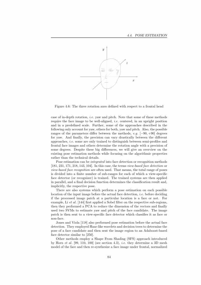
4.4. POSE ESTIMATION
x
y
z
Figure 4.6: The three rotation axes defined with respect to a frontal head
case of in-depth rotation, i.e. yaw and pitch. Note that some of these methodsrequire the face image to be well-aligned, i.e. centered, in an upright positionand in a predefined scale. Further, some of the approaches described in thefollowing only account for yaw, others for both, yaw and pitch. Also, the possibleranges of the parameters differ between the methods, e.g. [−90, +90] degreesfor yaw. And finally, the precision can vary drastically between the differentapproaches, i.e. some are only trained to distinguish between semi-profiles andfrontal face images and others determine the rotation angle with a precision ofsome degrees. Despite these big differences, we will give an overview on theexisting pose estimation methods while focusing on the algorithmic propertiesrather than the technical details.
Pose estimation can be integrated into face detection or recognition methods[181, 231, 171, 218, 143, 104]. In this case, the terms view-based face detection orview-based face recognition are often used. That means, the total range of posesis divided into a finite number of sub-ranges for each of which a view-specificface detector (or recognizer) is trained. The trained systems are then appliedin parallel, and a final decision function determines the classification result and,implicitly, the respective pose.
There are also systems which perform a pose estimation on each possiblelocation of the input image before the actual face detection, i.e. before decidingif the processed image patch at a particular location is a face or not. Forexample, Li et al . [144] first applied a Sobel filter on the respective sub-regions,then they performed a PCA to reduce the dimension of the vectors and finallyused two SVMs to estimate yaw and pitch of the face candidate. The imagepatch is then sent to a view-specific face detector which classifies it as face ornon-face.
Jones and Viola [118] also performed pose estimation before the actual facedetection. They employed Haar-like wavelets and decision trees to determine thepose of a face candidate and then sent the image region to an Adaboost-basedface detector similar to [250].
Other methods employ a Shape From Shading (SFS) approach introducedby Horn et al . [99, 110, 100] (see section 4.3), i.e. they determine a 3D meshmodel of the face and then re-synthesize a face image under frontal, normalized
84
CHAPTER 4. FACE DETECTION AND NORMALIZATION
pose. However, unless specific constraints are enforced on the algorithm, severalimages of the same face under different illumination are needed, which makesthis approach rather impractical in common face analysis applications.
A different approach based on linear object classes has been proposed byVetter et al . [248]. It is rather a pose normalization than a simple pose pa-rameter estimation method. The authors assumed that the 3D shape of anobject (and 2D projections of 3D objects) of a given view can be representedby a linear combination of prototypical objects (of the same view). It followsthat a rotated view of the object is a linear combination of the rotated viewsof the prototype objects. In this way, one can synthesize rotated views of faceimages from a single example view. In [21], this algorithm has been used in amulti-view face recognition system to create virtual views from a single inputimage. Lando and Edelman [129] used a comparable example-based techniquefor the same purpose.
The above mentioned methods are rather special cases of pose normaliza-tion techniques as they are either an integral part of a face detection/recognitionsystem or need several input face images, or they synthesize a face in a given(normalized) pose instead of estimating the underlying pose parameters. How-ever, the methods outlined in the following are pure pose estimation techniquesas they process face images and estimate the parameters of the correspondingpose of the face. These approaches can be divided into two main categories:feature-based and template-based (or appearance-based) methods.
Feature-based methods localize specific facial features and then comparethem with some probabilistic or geometric model in order to determine thehead pose. The method of Azarbayejani et al . [4], for example, detects featurepoints having a large Hessian w.r.t. image intensity assuming that these pointscorrespond to eye corners, pupils, nostrils etc. The authors applied their al-gorithm on videos and tracked the detected points using an Extended KalmanFilter (EKF).
Lee et al . [139] used a deformable 3D model composed of an edge model, acolor region model and a wireframe model in order to synthesize images of facesin arbitrary poses. An iterative energy minimization approach has been em-ployed to match the generic model to a given test face image and thus estimatethe corresponding head pose.
Chen et al . [38] proposed a method segmenting the two separate regions ofthe face and the hair respectively and then estimate the x, y and z rotation ofthe head using geometrical features of the two regions, such as area, center andaxis of least inertia.
Approaches based on Bunch Graph Matching (BGM) have been proposed byKruger et al . [127] and Elagin et al . [61]. Here, the local appearance of the faceshas been described with Gabor jets, i.e. set of Gabor wavelet filter responses,which are organized in a two-dimensional graph that is fit to the face image byminimizing a global energy function.
In a later work, Kruger et al . [126] presented a pose estimation approachsimilar to BGMs using Gabor Wavelet Networks (GWN). Unlike the separaterepresentation of the graph and the wavelets in BGMs, GWNs are able to si-multaneously encode the local appearance of the face image and geometricalproperties of local features. They used a Linear Local Map (LLM) [198], alinear approximation method related to Self-Organizing Maps and GeneralizedRadial Basis Functions, for a final classification step.
85
4.5. FACE ALIGNMENT
Lanitis et al . [131] presented a pose estimation method based on ActiveShape Models where a statistical model of the shape of a face using landmarkpoints is iteratively fit to the face image (see section 2.3).
In contrast to feature-based approaches, template-based methods do notlocalize specific facial features but treat the face image as a whole. Schiele etal . [217], for example, presented a method where the face region is segmentedfrom the background and the hair regions by a skin-color-based segmentationalgorithm. The pose was then estimated by a MLP that classifies the resultingpattern. MLPs have also been used by Zhao et al . [270] and Brown et al . [31].
Huang et al . [105] use SVMs for left/right/frontal pose classification. Intheir approach, one SVM for each pose was trained on the raw face images andwith two different kernels, a polynomial and a RBF kernel.
Rae et al . [192] proposed a method that filters the face images with Gaborwavelets placed on a circular grid on the input image and then classifies therespective head pose by a LLM.
McKenna et al . [159] also presented a method based on Gabor Waveletfilters. The head pose was classified by comparing the resulting filtered imagewith a certain number of template images, each corresponding to a certain yawand pitch.
Baluja [10] classified five different head poses by different probabilistic mod-els, e.g. a Naive-Bayes model, which was built using labeled and unlabeled bina-rized face images. Another approach, presented by Ba et al . [5], uses GaussianMixture Models (GMM) to represent the different head poses.
Niyogi and Freeman [172] employed a template matching technique based ona vector quantization method called Tree-Structured Vector Quantizer (TSVQ),i.e. the training examples (the templates) together with their respective posewere organized in a tree-like structure using PCA and clustering.
Other methods are based on the concept of Pose Eigenspace (PES) [87]which is a linear sub-space spanned by the first three eigenvectors of the faceimages’ covariance matrix. These three directions are assumed to account forthe majority of appearance variations due to changing pose. Further, a faceimage with varying pose represents a continuous manifold in this sub-space.The method proposed by Motwani [166] builds a PES with wavelet filtered faceimages and classifies face pose by calculating the Euclidean distance betweenthe projected vectors of given test image and the training images respectively.Wei et al . [256] also used a PES-based approach using Gabor wavelet filters anda Mahalanobis distance measure.
Finally, a different approach based on Dynamic Space Warping (DSW) hasbeen proposed by Yegnanarayana et al . [267]. Here, a face image under a givenpose is horizontally warped to best match a frontal face and the respectivewarping path is analyzed in order to estimate the yaw pose angle.
4.5 Face Alignment
4.5.1 Introduction
Face alignment or face registration designates a normalization procedure wherethe bounding boxes coming from a face detector are transformed in such away that the faces are well aligned with them. “Well aligned” means most
86

CHAPTER 4. FACE DETECTION AND NORMALIZATION
translation
scalerotation
Figure 4.7: The face alignment process
often: centered and in a predefined scale and orientation. Figure 4.7 illustratesthis procedure. Thus, the transformation is in most cases affine and the faceimages cropped along the boundaries of the resulting rectangles have specificfacial features, such as eyes, nose, mouth, approximately at predefined relativepositions in the image.
This step is crucial for further effective face analysis, e.g. face recognition.Shan et al . [224] and Rentzeperis et al . [196] showed that slight mis-alignments,i.e. x and y translation, rotation or scale changes, cause a considerable perfor-mance drop of most of the current face recognition methods.
There have been different approaches to overcome the mis-alignment prob-lem in face recognition. Shan et al . [224], for example, added virtual exampleswith small transformations to the training set of the face recognition systemand, thus, made it more robust. Martinez [153] additionally modeled the distri-bution in the feature space under varying translation by a mixture of Gaussians.However, these approaches can only cope with relatively small variations.
4.5.2 State-of-the-art
Existing approaches can be divided into two main groups: approaches based onfacial feature detection and global matching approaches, most of the publishedmethods belonging to the first group.
Berg et al . [20], for example, used a SVM-based feature detector to detecteye and mouth corners and the nose and then applied an affine transformationto align the face images such that eye and mouth centers are at predefinedpositions. Wiskott et al . [260] used a technique called Elastic Bunch GraphMatching (EBGM) where they mapped a deformable grid onto a face image byusing local sets of Gabor filtered features. Numerous other methods [8, 60, 103,143] align faces by means of approaches derived from the Active AppearanceModels introduced by Cootes et al . [41] (see section 2.3).
Approaches belonging to the second group are less common. Moghaddamet al . [165], for example, used a maximum likelihood-based template matchingmethod to eliminate translation and scale variations. In a second step, however,they detected four facial features to correct rotation as well. Jia et al . [117]employed a tensor-based model to super-resolve face images of low resolution,and at the same time find the best alignment by minimizing the correlationbetween the low-resolution image and the super-resolved one. Rowley et al . [207]proposed a face detection method including a Multi-Layer Perceptron (MLP) toestimate in-plane face rotation of arbitrary angle. They perform the alignment
87
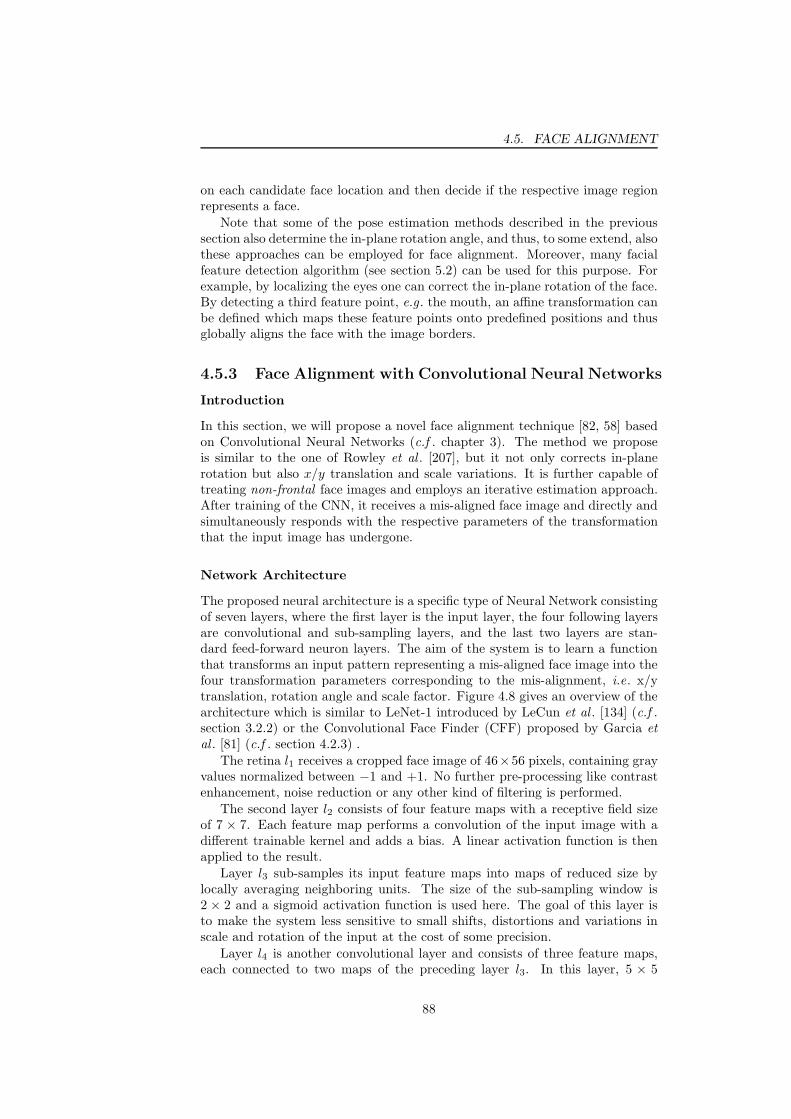
4.5. FACE ALIGNMENT
on each candidate face location and then decide if the respective image regionrepresents a face.
Note that some of the pose estimation methods described in the previoussection also determine the in-plane rotation angle, and thus, to some extend, alsothese approaches can be employed for face alignment. Moreover, many facialfeature detection algorithm (see section 5.2) can be used for this purpose. Forexample, by localizing the eyes one can correct the in-plane rotation of the face.By detecting a third feature point, e.g. the mouth, an affine transformation canbe defined which maps these feature points onto predefined positions and thusglobally aligns the face with the image borders.
4.5.3 Face Alignment with Convolutional Neural Networks
Introduction
In this section, we will propose a novel face alignment technique [82, 58] basedon Convolutional Neural Networks (c.f . chapter 3). The method we proposeis similar to the one of Rowley et al . [207], but it not only corrects in-planerotation but also x/y translation and scale variations. It is further capable oftreating non-frontal face images and employs an iterative estimation approach.After training of the CNN, it receives a mis-aligned face image and directly andsimultaneously responds with the respective parameters of the transformationthat the input image has undergone.
Network Architecture
The proposed neural architecture is a specific type of Neural Network consistingof seven layers, where the first layer is the input layer, the four following layersare convolutional and sub-sampling layers, and the last two layers are stan-dard feed-forward neuron layers. The aim of the system is to learn a functionthat transforms an input pattern representing a mis-aligned face image into thefour transformation parameters corresponding to the mis-alignment, i.e. x/ytranslation, rotation angle and scale factor. Figure 4.8 gives an overview of thearchitecture which is similar to LeNet-1 introduced by LeCun et al . [134] (c.f .section 3.2.2) or the Convolutional Face Finder (CFF) proposed by Garcia etal . [81] (c.f . section 4.2.3) .
The retina l1 receives a cropped face image of 46×56 pixels, containing grayvalues normalized between −1 and +1. No further pre-processing like contrastenhancement, noise reduction or any other kind of filtering is performed.
The second layer l2 consists of four feature maps with a receptive field sizeof 7 × 7. Each feature map performs a convolution of the input image with adifferent trainable kernel and adds a bias. A linear activation function is thenapplied to the result.
Layer l3 sub-samples its input feature maps into maps of reduced size bylocally averaging neighboring units. The size of the sub-sampling window is2 × 2 and a sigmoid activation function is used here. The goal of this layer isto make the system less sensitive to small shifts, distortions and variations inscale and rotation of the input at the cost of some precision.
Layer l4 is another convolutional layer and consists of three feature maps,each connected to two maps of the preceding layer l3. In this layer, 5 × 5
88

CHAPTER 4. FACE DETECTION AND NORMALIZATION
Translation Y
Scale factor
Translation X
Rotation angle
convolution 7x7
convolution 5x5
subsamplingsubsampling
l1: 1x46x56
l2: 4x40x50
l3: 4x20x25
l4: 3x16x21
l5: 3x8x10
l6: 40
l7: 4
Figure 4.8: The Neural Network architecture of the proposed face alignmentsystem
convolution kernels are used, and each feature map has two different convolutionkernels, one for each input map. The results of the two convolutions as well asthe bias are simply added up. The maps of layer l4 extract higher-level featuresby combining the lower-level information in l2.
Layer l5 is again a sub-sampling layer that works the same way as l3, i.e. itreduces the size of the feature maps again by a factor of two.
Whereas the previous layers act principally as feature extraction layers, lay-ers l6 and l7 combine the extracted local features into a global model. Theyare neuron layers that are fully connected to their respective preceding layersand use a sigmoid activation function. l7 is the output layer containing exactlyfour neurons, representing x and y translation, rotation angle and scale fac-tor, normalized between −1 and +1 w.r.t. their minimum and maximum valuespmini and pmaxi, e.g. ±30 degrees for the rotation angle. After activationof the network, these neurons contain the estimated normalized transformationparameters y7i (i = 1..4) of the mis-aligned face image presented at l1. Eachfinal transformation parameter pi is then calculated by linearly rescaling thecorresponding y7i value from [-1,+1] to the interval of the respective minimaland maximal allowed values pmini and pmaxi:
pi =pmaxi − pmini
2(y7i + 1) + pmini , ∀i = 1..4 . (4.1)
89

4.5. FACE ALIGNMENT
Figure 4.9: Examples of training images created by manually mis-aligning theface (top left: the well-aligned face image)
Training Process
We constructed a training set of about 30,000 face images extracted from severalpublic face databases with annotated eye, nose and mouth positions. Using theannotated facial features, we are able to crop well-aligned face images where theeyes and the mouth are roughly at predefined positions while keeping a constantaspect ratio. By applying transformations on the well aligned face images, weproduced a set of artificially mis-aligned face images, that we cropped fromthe original images and resized to the dimensions of the retina (46× 56). Thetransformations were applied by varying translation between −6 and +6 pixels,rotation between −30 and +30 degrees and the scale factor between 0.9 and 1.1.Thus, we defined the minimal and maximal parameter values as follows:
pmin1 = pmin2 = −6
pmax1 = pmax2 = +6
pmin3 = −30
pmax3 = +30
pmin4 = 0.9
pmax4 = 1.1
Figure 4.9 shows some training examples for one given face image. The respec-tive transformation parameters pi were stored for each training example andused to define the corresponding desired outputs ti of the Neural Network bynormalizing them between −1 and +1:
ti =2× (pi − pmini)
pmaxi − pmini
− 1 , i = 1..4 . (4.2)
Training was performed using the well-known Backpropagation algorithmwhich has been adapted in order to account for weight sharing in the convolu-tional layers (l2 and l4) (see Alg. 8 on page 57). The objective function is simplythe Mean Squared Error (MSE) between the computed outputs and the desiredoutputs of the four neurons in l7 for all N training examples:
E =1
4N
N∑
k=1
4∑
i=1
(y7i − ti)2
. (4.3)
At each iteration, a set of 1,000 face images is selected at random. Then, eachface image example of this set and its known transformation parameters are
90

CHAPTER 4. FACE DETECTION AND NORMALIZATION
Face Detection
Alignment estimationby CNN
Translation Y = +4Rotation angle = −14Scale factor = 0.95
Translation X = − 2
Adjust by 10% usingthe inverse parameters
30 iterations ?
Face extractionand rescaling
Save finalparameters
no
yes
Figure 4.10: The overall face alignment procedure of the proposed system
presented, one at a time, to the Neural Network and the weights are updatedaccordingly (online training). Classically, in order to avoid overfitting, aftereach training iteration, a validation phase is performed using a separate vali-dation set. A minimal error on the validation set is supposed to give the bestgeneralization and the corresponding weight configuration is stored.
Alignment Process
We now explain how the Neural Network is used to align face images with bound-ing boxes obtained from a face detector. The overall procedure is illustrated infigure 4.10. Face detection is performed using the Convolutional Face Finderof Garcia and Delakis [81] (c.f . section 4.2.3) which produces upright boundingboxes. The detected faces are then extracted according to the bounding boxand resized to 46× 56 pixels. For each detected face, the alignment process isperformed by presenting the mis-aligned cropped face image to the trained Neu-ral Network which in turn gives an estimation of the underlying transformation.
91

4.5. FACE ALIGNMENT
A correction of the bounding box can then simply be achieved by applying theinverse transformation parameters (−pi for translation and rotation and 1/pi
for scale). However, in order to improve the correction, this step is performedseveral (e.g. 30) times in an iterative manner, where, at each iteration, only acertain proportion (e.g. 10%) of the correction is applied to the bounding box.At each step, the face image is re-cropped using the new bounding box and anew estimation of the parameters is calculated with this modified image. Thetransformation with respect to the initial bounding box is obtained by simplyaccumulating the respective parameters at each iteration. Using this iterativeapproach the system finally converges to a more precise solution than whenusing a full one-step correction.
The alignment precision can be further improved by successively executingthe procedure described above two times with two different Neural Networks,the first one trained as presented above for coarse alignment and the second onefor fine alignment. For training the fine alignment Neural Network, we builta set of face images with less variation, i.e. [−2, +2] for x and y translations,[−10, +10] for rotation and [0.95, 1.05] for scale variation. The parameters pmini
and pmaxi (i = 1..4) change accordingly in the preceding formulas.
Experimental Results
To evaluate the proposed approach, we used two different annotated test sets:the public face database BioID [22] containing 1,520 images and a private setof about 200 images downloaded from the Internet (see Appendix A). Thelatter, referred to as Internet test set, contains face images of varying size, withlarge variations in illumination, pose, facial expressions and containing noise andpartial occlusions. As described in the previous section, for each face localized bythe face detector [81], we perform the alignment on the respective bounding boxand calculate the precision error e which is defined as the mean of the distancesbetween its corners ai and the respective corners of the desired bounding boxdi normalized with respect to the width W of the desired bounding box:
e =1
4W
4X
i=1
‖ai − di‖ (4.4)
Figure 4.11 shows, for the two test sets, the proportion of correctly alignedfaces varying the allowed error e.
For example, if we allow an error of 10% of the bounding box width, 80%and 94% of the faces of the Internet and BioID test sets respectively are wellaligned. Further, for about 70% of the aligned BioID faces, e is below 5%.
We also compared our approach to a different technique that localizes theeye centers, the nose tip and the mouth center. This method is also basedon CNNs and described in section 5.3. The face images with localized facialfeatures are aligned using the same formula as used for creating the training setof the Neural Network presented in this paper. Figure 4.12 shows the respectiveresults for the Internet test set.
To show the robustness of the proposed method, we added Gaussian noisewith varying standard deviation σ to the pixels of the input images beforeperforming face alignment. Figure 4.13 shows the error e versus σ, averagedover the whole set for both of the test sets. Note that e remains below 14% for
92
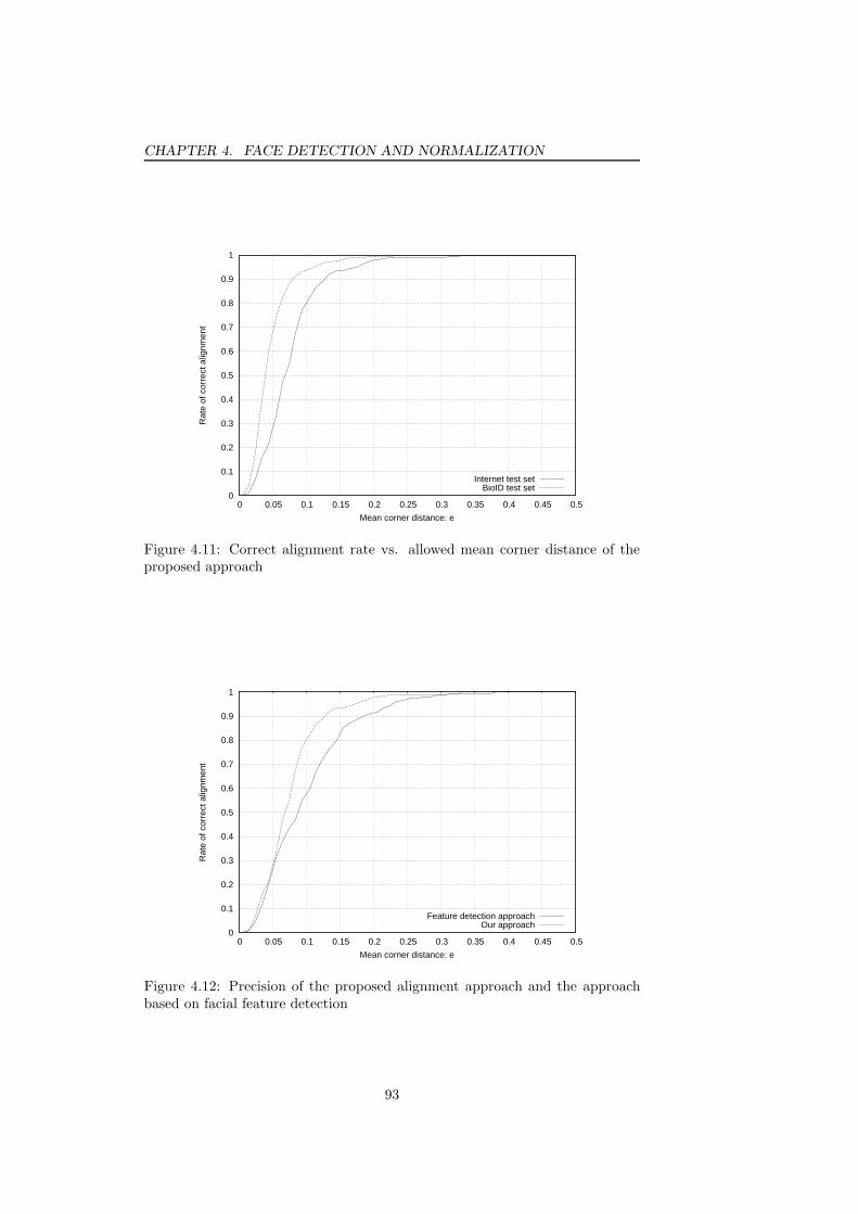
CHAPTER 4. FACE DETECTION AND NORMALIZATION
0
0.1
0.2
0.3
0.4
0.5
0.6
0.7
0.8
0.9
1
0 0.05 0.1 0.15 0.2 0.25 0.3 0.35 0.4 0.45 0.5
Rat
e of
cor
rect
alig
nmen
t
Mean corner distance: e
Internet test setBioID test set
Figure 4.11: Correct alignment rate vs. allowed mean corner distance of theproposed approach
0
0.1
0.2
0.3
0.4
0.5
0.6
0.7
0.8
0.9
1
0 0.05 0.1 0.15 0.2 0.25 0.3 0.35 0.4 0.45 0.5
Rat
e of
cor
rect
alig
nmen
t
Mean corner distance: e
Feature detection approachOur approach
Figure 4.12: Precision of the proposed alignment approach and the approachbased on facial feature detection
93
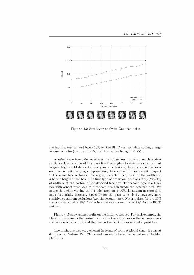
4.5. FACE ALIGNMENT
0
0.05
0.1
0.15
0.2
0 20 40 60 80 100 120 140
mea
n e
standard deviation
InternetBioID
Figure 4.13: Sensitivity analysis: Gaussian noise
the Internet test set and below 10% for the BioID test set while adding a largeamount of noise (i.e. σ up to 150 for pixel values being in [0, 255]).
Another experiment demonstrates the robustness of our approach againstpartial occlusions while adding black filled rectangles of varying area to the inputimages. Figure 4.14 shows, for two types of occlusions, the error e averaged overeach test set with varying s, representing the occluded proportion with respectto the whole face rectangle. For a given detected face, let w be the width andh be the height of the box. The first type of occlusion is a black strip (“scarf”)of width w at the bottom of the detected face box. The second type is a blackbox with aspect ratio w/h at a random position inside the detected box. Wenotice that while varying the occluded area up to 40% the alignment error doesnot substantially increase, especially for the scarf type. It is, however, moresensitive to random occlusions (i.e. the second type). Nevertheless, for s < 30%the error stays below 15% for the Internet test set and below 12% for the BioIDtest set.
Figure 4.15 shows some results on the Internet test set. For each example, theblack box represents the desired box, while the white box on the left representsthe face detector output and the one on the right the estimated aligned box.
The method is also very efficient in terms of computational time. It runs at67 fps on a Pentium IV 3.2GHz and can easily be implemented on embeddedplatforms.
94

CHAPTER 4. FACE DETECTION AND NORMALIZATION
0
0.05
0.1
0.15
0.2
0 0.05 0.1 0.15 0.2 0.25 0.3 0.35 0.4
mea
n e
occluded porportion s
Internet: random rectangleInternet: scarf
BioID: random rectangleBioID: scarf
0
0.05
0.1
0.15
0.2
0 0.05 0.1 0.15 0.2 0.25 0.3 0.35 0.4
mea
n e
occluded porportion s
Internet: random rectangleInternet: scarf
BioID: random rectangleBioID: scarf
Figure 4.14: Sensitivity analysis: partial occlusion
4.6 Conclusion
In this chapter, we presented the problem of face detection in images and some ofthe most important approaches proposed in the literature to tackle this problem.Many face detection methods obtain relatively good results on standard publicface databases, like the CMU database. However, we focused on one approachin particular, the Convolutional Face Finder (CFF) of Garcia and Delakis [81]as it is a CNN-based method and it attains a high detection rate with a lowfalse alarm rate, which is a very desirable property in face detection. Its highperformance in terms of computation time and the ability to implement it onembedded platforms are further advantages of this approach.
We then pointed out that for further face analysis tasks, notably for facerecognition, a preceding normalization step is essential and we described possiblemethods employed in this context, such as illumination normalization and headpose estimation and/or correction. In this regard, we outlined some well-knownapproaches published in the literature.
Finally, we proposed a novel face alignment method which can be consideredas a post-processing step of face detection. It is based on CNNs and trained tosimultaneously estimate x/y translation as well as rotation and scale variationsof the slightly mis-aligned bounding rectangles coming from a face detector.Experimental results show that this approach is precise and very robust whenapplied to face images under difficult illumination conditions and varying headpose. Also, a considerable robustness to pixel-noise and partial occlusions hasbeen experimentally verified.
The combination of CFF and the face alignment system shows to perform
95

4.6. CONCLUSION
Figure 4.15: Some alignment results on the Internet test set. For each testimage, the black rectangle represents the desired bounding box. The whiterectangle on the respective left image shows the output of the face detector andthe white rectangle on the right image shows the result of the face alignmentsystem.
96

CHAPTER 4. FACE DETECTION AND NORMALIZATION
very well in real-world contexts of facial image processing applications underdifficult conditions. Further, the efficient implementation, also on embeddedplatforms, make them a powerful technique suitable for further facial analysissuch as face recognition.
97
Chapter 5
Facial Feature Detection
5.1 Introduction
Facial feature detection designates the problem of localizing characteristic pointsin face images, such as the eyes, the nose tip, the mouth, the corners of themouth etc. Depending on the resolution of the face images being processed thelocalization can also imply more specific features, e.g. eye corners, eye browcorners, orbit points, nostrils or points marking the chin. This is sometimesalso referred to as fiducial point detection.
Facial feature detection algorithms differ in several aspects. First of all, theycan be part of a face detection method where the feature detectors scan over alarger image which may contain a face or not. Then, the presence of all or mostof the facial features at a given location and a plausible constellation of themindicate the presence of a face at this particular position. Many facial featuredetection algorithms, however, operate on images or image regions containingonly the face which have been localized and extracted beforehand by a facedetection algorithm. A further point where the algorithms differ is the type ofimage they are working on. This implies the image resolution as well as externalconditions such as illumination, noise, background but also the range of possiblehead poses and facial expressions. Another important aspect is the purpose orthe target application of the respective feature detection algorithm as this mightimpose more or less strict precision constraints as well as the type and numberof features to detect. As mentioned above, they can be part of a face detectionsystem, for example, which in turn can be part of a larger face processing system.Other possible applications are facial expression recognition or face recognitionrequiring a rather precise localization of specific facial features. Finally, it maybe used for advanced Human-Computer Interaction (HCI) applications, e.g.avatar animation.
The problem of facial feature detection under unconstrained conditions isstill far from being resolved, and the difficulties that remain are essentially thesame as for face analysis tasks in general, notably those outlined in section 1.3,e.g. the sensitivity to illumination and pose variations, facial expressions andpartial occlusions.
In the following, we will describe some of the most important works in thisfield and then present our own approach to facial feature detection using Convo-
98

CHAPTER 5. FACIAL FEATURE DETECTION
lutional Neural Networks. Finally, we will experimentally show the performanceof the proposed method in terms of detection rate and precision as well as therobustness against the types of noise mentioned above.
5.2 State-of-the-art
Numerous approaches to facial feature detection in still images have been pro-posed in the last decade. One could classify them into two categories: the firstcategory applies local processing techniques to the face image, such as filtersor templates, in order to obtain candidate feature positions and then selectsthe most likely combination (or the one with the highest score) w.r.t. a globalmodel. Approaches belonging to the second category iteratively try to matcha grid, a graph or any other form of deformable global model to a face image.The algorithms of this category are supposed to converge to a solution wherethe grid points correspond to the facial features to localize.
Local feature detection approaches
Vincent et al . [249] proposed a system detecting eye and mouth features usingseveral trained Multi-Layer Perceptrons (MLP) for each feature to detect scan-ning over the input image. In a coarse-to-fine approach, they first localized theeye and mouth features and then 12 so-called “micro-features”, five for each eyeand two for the mouth. Finally, a maximum likelihood estimator provides themost likely combination of features.
Reinders et al . [194] presented a similar approach using a MLP working ongradient magnitudes and orientations in order to detect the rough eye positionsand then four specialized MLPs to detect micro-features.
Yuille et al . [269] presented a technique based on deformable templates ofthe eye and the mouth. The feature localization was performed by fitting theparameterized templates to image locations where a specific energy functionis minimal. The function was based on edges, peaks and valleys of the imageintensity.
Other works are based on skin-color segmentation [210, 83, 229, 88], contrastenhancement and thresholding techniques [115] and/or symmetry measures [195,111, 210] which, in practice, show to be rather sensitive to noise and illuminationchanges.
Leung et al . [141] used multi-orientation, multi-scale Gaussian derivativefilters to detect feature position candidates in the input image. The best matcheswere retained, and for each pair of detected feature point they estimated smallelliptical regions where the rest of the feature points to detect are likely to occur.In the following step, a probabilistic model based on mutual feature distanceshelped to identify the most likely feature positions.
Yow and Cipolla [268] also used Gaussian derivate filters to detect facial fea-ture candidates. However, a grouping method based on belief networks was thenapplied to the candidate positions in order to obtain the resulting combinationof facial features.
A method based on Eigen-features was presented by Moghaddam et al . [165].Here, the residual error between the image patch in the search window and thereconstructed image, the so-called Distance From Feature Space (DFFS), was
99
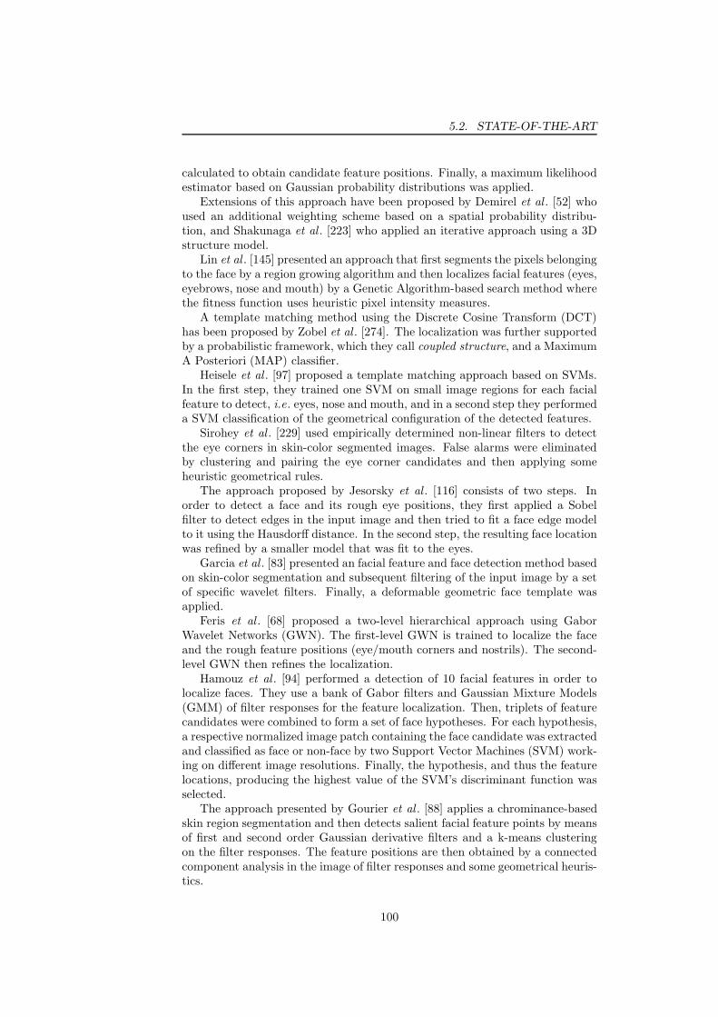
5.2. STATE-OF-THE-ART
calculated to obtain candidate feature positions. Finally, a maximum likelihoodestimator based on Gaussian probability distributions was applied.
Extensions of this approach have been proposed by Demirel et al . [52] whoused an additional weighting scheme based on a spatial probability distribu-tion, and Shakunaga et al . [223] who applied an iterative approach using a 3Dstructure model.
Lin et al . [145] presented an approach that first segments the pixels belongingto the face by a region growing algorithm and then localizes facial features (eyes,eyebrows, nose and mouth) by a Genetic Algorithm-based search method wherethe fitness function uses heuristic pixel intensity measures.
A template matching method using the Discrete Cosine Transform (DCT)has been proposed by Zobel et al . [274]. The localization was further supportedby a probabilistic framework, which they call coupled structure, and a MaximumA Posteriori (MAP) classifier.
Heisele et al . [97] proposed a template matching approach based on SVMs.In the first step, they trained one SVM on small image regions for each facialfeature to detect, i.e. eyes, nose and mouth, and in a second step they performeda SVM classification of the geometrical configuration of the detected features.
Sirohey et al . [229] used empirically determined non-linear filters to detectthe eye corners in skin-color segmented images. False alarms were eliminatedby clustering and pairing the eye corner candidates and then applying someheuristic geometrical rules.
The approach proposed by Jesorsky et al . [116] consists of two steps. Inorder to detect a face and its rough eye positions, they first applied a Sobelfilter to detect edges in the input image and then tried to fit a face edge modelto it using the Hausdorff distance. In the second step, the resulting face locationwas refined by a smaller model that was fit to the eyes.
Garcia et al . [83] presented an facial feature and face detection method basedon skin-color segmentation and subsequent filtering of the input image by a setof specific wavelet filters. Finally, a deformable geometric face template wasapplied.
Feris et al . [68] proposed a two-level hierarchical approach using GaborWavelet Networks (GWN). The first-level GWN is trained to localize the faceand the rough feature positions (eye/mouth corners and nostrils). The second-level GWN then refines the localization.
Hamouz et al . [94] performed a detection of 10 facial features in order tolocalize faces. They use a bank of Gabor filters and Gaussian Mixture Models(GMM) of filter responses for the feature localization. Then, triplets of featurecandidates were combined to form a set of face hypotheses. For each hypothesis,a respective normalized image patch containing the face candidate was extractedand classified as face or non-face by two Support Vector Machines (SVM) work-ing on different image resolutions. Finally, the hypothesis, and thus the featurelocations, producing the highest value of the SVM’s discriminant function wasselected.
The approach presented by Gourier et al . [88] applies a chrominance-basedskin region segmentation and then detects salient facial feature points by meansof first and second order Gaussian derivative filters and a k-means clusteringon the filter responses. The feature positions are then obtained by a connectedcomponent analysis in the image of filter responses and some geometrical heuris-tics.
100
CHAPTER 5. FACIAL FEATURE DETECTION
Iterative methods using deformable grids
Whereas the approaches of the preceding section could be denoted as “bottom-up”, the methods outlined in the following can be considered as “top-down”approaches because a global model, i.e. a deformable grid, is fit to the face imageby some kind of iterative optimization technique operating on local appearances.
The first very well-known method of this type has been presented by Wiskottet al . [260] and is called Elastic Bunch Graph Matching (EBGM). As this ap-proach is not only used for feature detection but also for face recognition it willbe described in section 6.2.
More recently, Cootes et al . [41] introduced a technique called Active Ap-pearance Models (AAM) (see section 2.3). By applying Principal ComponentAnalysis (PCA) on the training set of faces with manually labeled feature po-sitions they first constructed a statistical shape model. Then, the face imageswere warped to fit the mean shape and a second PCA on the so-called shape-free patches was performed in order to obtain an independent statistical texturemodel. To localize facial features in a new face image, the respective parame-ters of the shape and texture models are iteratively estimated minimizing theresidual textural error between model and estimation. Note that, in order towork effectively, methods based on AAMs need a rather good initialization offeature positions.
Cristinacce and Cootes [49] proposed a method to detect 17 facial featurepoints. First, they applied the face detector presented by Viola and Jones [250],they resized the extracted face image to 100×100 pixels and then computed a so-called feature response image. This image contains at each location (i.e. pixel)the result of an Adaboost classifier combining three different feature extractors:one based on normalized eye and mouth templates, one based on orientationmaps and the third using Boosted Cascade Detectors. Finally, the feature lo-cations were determined by a non-linear optimization method, which they callShape Optimized Search (SOS). It uses a statistical shape model, initially com-puted by PCA, and a fitting function taking into account both shape and theresponse of the feature extractors, i.e. the feature response image.
In another work [50], Cristinacce et al . proposed a feature detection tech-nique using Boosted Cascade Detectors [250] and also a statistical model. Theyfirst localized the face and facial features with the Boosted Cascade Detectorstrained on appropriate image patches. Then, they modeled the pairwise condi-tional distribution of feature positions using histograms, a technique which theycall “Pairwise Reinforcement of Feature Responses” (PRFR). Finally, an AAMvariant due to Scott et al . [221] was used to refine the feature positions. Theyshowed that this method outperforms their previous work [49] as well as purelyAAM-based methods [41].
Evaluation
The comparison of the performance of feature detection approaches outlined theprevious sections is rather difficult as the authors used different and often privateface databases to evaluate their methods. Moreover, not all methods detectthe same facial features and/or the same number of features. Nevertheless,an overview of the performance of some facial feature detection methods ispresented in table 5.1. The allowed error in the last column represents the error
101

5.2. STATE-OF-THE-ART
threshold normalized w.r.t. the inter-ocular distance. A question mark signifiesthat the allowed error has not been reported in the paper. In this case, thedetection rate does not tell very much about the precision of the respectivemethods.
Author Database Facial Features
Detec-
tion
rate
Allowed
error
Leung [141] private eyes,nose (5 pts.) 86% ?
Reinders [194] private right eye (4 pts.) 96% 10%
Shakunaga [223] privateeyes,nose,mouth
96% ?ears (8 pts.)
Jesorsky [116]BIOID [22]
eyes (2 pts.)80% 10%
XM2VTS [160] 92% 10%
Sirohey [229] Aberdeen [185] eyes (4 pts.) 90% ?
Feris [68] Yale[16],FERET[183]eyes (4 pts.) 95% ≈ 5%
nostrils (2 pts.) 95% ≈ 5%mouth (2 pts.) 88% ≈ 5%
Cristinacce [49] BIOID [22]eyes,nose,mouth 85% 10%
(17 pts.) 96% 15%
Gourier [88] privateeyes (2 pts.) 97% ?
mouths (1 pt.) 88.8% ?
Hamouz [94]BIOID [22]
eyes,nose,mouth(10 pts.)
76% 5%XM2VTS [160] 88% 5%
BANCA [7] 81.4% 5%
Table 5.1: Overview of detection rates of some published facial feature detectionmethods
For an allowed error of about 5%, the approach proposed by Feris et al .[68] shows good results on set of images from the Yale [16] and FERET [183]databases. And for an allowed error of 10%, Jesorsky et al . [116] obtain ac-ceptable results on the BioID [22] and the XM2VTS [160] databases. Reinderset al . [194] also report a good detection rate. However, their method only de-tects eye features, and unfortunately they used a private database. Finally, verygood results have been obtained by the approach proposed by Cristinacce andCootes [49], i.e. 96% with 15% allowed error and 85% with 10% allowed error,considering the rather difficult database BioID they used. Refer to Appendix Afor excerpts from some of these databases.
Up to the present, most of the published approaches have been evaluatedon face databases containing images taken under rather constrained conditions.In contrast to these methods, we will propose a novel system based on Con-volutional Neural Networks that is able to precisely and robustly detect facialfeatures under less constrained conditions.
102
CHAPTER 5. FACIAL FEATURE DETECTION
5.3 Facial Feature Detection with Convolutional
Neural Networks
5.3.1 Introduction
We propose a hierarchical neural-based facial feature detection scheme whichis designed to precisely locate fine facial features in faces of variable size andappearance, rotated up to ±30 degrees in the image plane and turned up to±60 degrees, in complex still gray-scale images [53, 54, 82, 59]. Using stillgray-scale images makes the approach more generic but also more challengingas skin color or motion clue cannot be used to aid detection. The system wepresent is able to detect facial features in very complex images taken under awide variety of poses, in low resolution images, with partial occlusions, noise andextreme lighting variations. The proposed approach is divided into three stages;in the first stage, faces contained in the image are automatically located. Thesecond stage consists in finding the approximate positions of local facial featureswithin the detected face regions. In a final stage, these feature positions andtheir surrounding image regions are used to locate finer facial features.
The face detector as well as the coarse and fine feature detectors are basedon a specific architecture of convolutional and hetero-associative neural layers.They consist of several different neural network components forming a pipelineof specialized image transformations, learned automatically from a training setof faces with annotated facial features. All components of a feature detectorare sequentially connected and can thus be trained by simply presenting theinput image and desired output, i.e. feature positions. Global constraints ormodels are automatically learned and used implicitly in the detection process.After training, the facial feature detection system acts like a pipeline of simpleconvolution and sub-sampling modules that treat the raw input face image asa whole and build facial feature maps where facial feature positions are easilyretrieved.
5.3.2 Architecture of the Facial Feature Detection System
The proposed system consists of a number of independent detection componentsoperating in a hierarchical way and on different parts of the image (see Fig. 5.1).The first component performs automatic face detection using the “ConvolutionalFace Finder” (CFF) proposed by Garcia and Delakis [81] (see section 4.2.3)which detects faces and finds the respective detected face bounding boxes in theinput images.
The proposed Facial Feature Detector (FFD) processes the previously ex-tracted face regions and locates four facial features: the eye centers, the tip ofthe nose and the center of the mouth. Then, the eye and mouth regions areprocessed by a specialized Eye Feature Detector (EFD) and a Mouth FeatureDetector (MFD) which locate finer facial features; the EFD is designed to detectthe eye corners and the pupil, and the MFD is designed to detect the left andright corner of the mouth and the center points on the outer edges of the upperand lower lip.
103
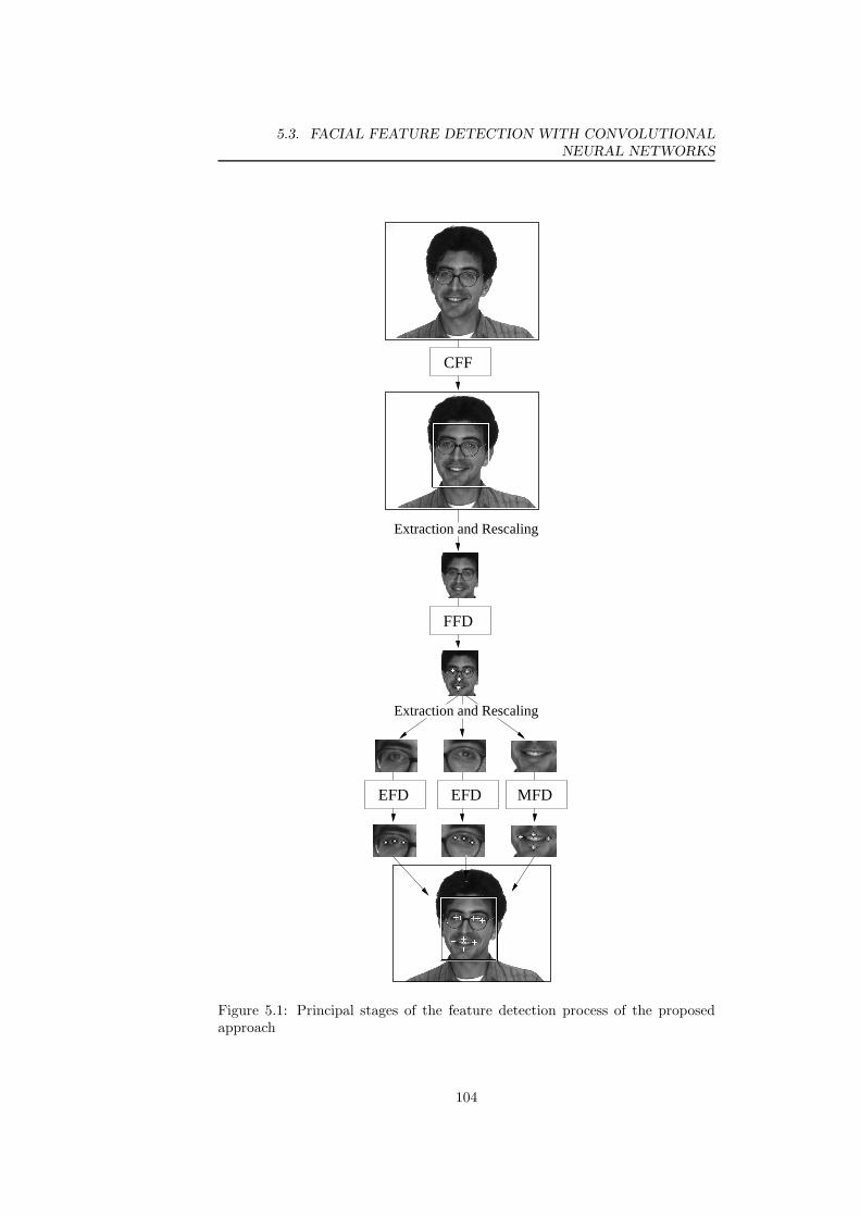
5.3. FACIAL FEATURE DETECTION WITH CONVOLUTIONAL
NEURAL NETWORKS
FFD
Extraction and Rescaling
Extraction and Rescaling
MFDEFDEFD
CFF
Figure 5.1: Principal stages of the feature detection process of the proposedapproach
104

CHAPTER 5. FACIAL FEATURE DETECTION
Figure 5.2: Some input images and corresponding desired output feature maps(right eye, left eye, nose tip and mouth center). For illustration purposes, thelast column shows the superposition of the desired outputs and the image atthe bottom shows an enlarged area of one of the desired feature maps
The Initial Facial Feature Detector
The architecture of the initial Facial Feature Detector (FFD) is a specific type ofConvolutional Neural Network (CNN) (c.f . chapter 3) consisting of six layers,where the first layer is the input layer, the three following layers are convo-lutional and sub-sampling layers, and the last two layers are standard feed-forward neuron layers. The aim of the system is to learn a non-linear functionthat transforms a raw input face image into desired output feature maps wherefacial features are highlighted (see Fig. 5.2).
Figure 5.3 gives an overview of the FFD architecture. The retina l1 receives acropped face image of 46×56 pixels, containing gray values normalized between−1 and +1. No further pre-processing such as contrast enhancement, noisereduction or any other kind of filtering is performed by the retina. The secondlayer l2 consists of four feature maps each having a 7× 7 trainable kernel anda linear activation function. Layer l3 is a sub-sampling layer with window size2 × 2 and sigmoid activation function. Layer l4 is another convolutional layerand consists of only one feature map with a 5× 5 kernel and sigmoid activationfunction.
While the previous layers act principally as feature extraction layers, layersl5 and l6 use the local information to form a global model. Layer l5 is composedof sigmoidal neurons fully connected to layer l4 and is dedicated to learningmodels (or constellations) of features and to activate the targeted positionsin the output feature maps. This part of the network was inspired by Auto-Associative Neural Networks (AANN) (c.f . section 2.8.4) which are trained toreproduce an input (pattern) by means of a hidden layer containing much lessneurons than the input dimension. It has been shown that AANNs effectivelyperform a dimensionality reduction similar to the one produced by a PrincipalComponent Analysis (PCA). In our case, we do not want to reproduce the inputbut rather to associate the output of the feature map in l4 with the desiredoutput in l6. In that way, we only allow certain constellations of features inlayer l6 to be activated. This global processing step makes the system less
105
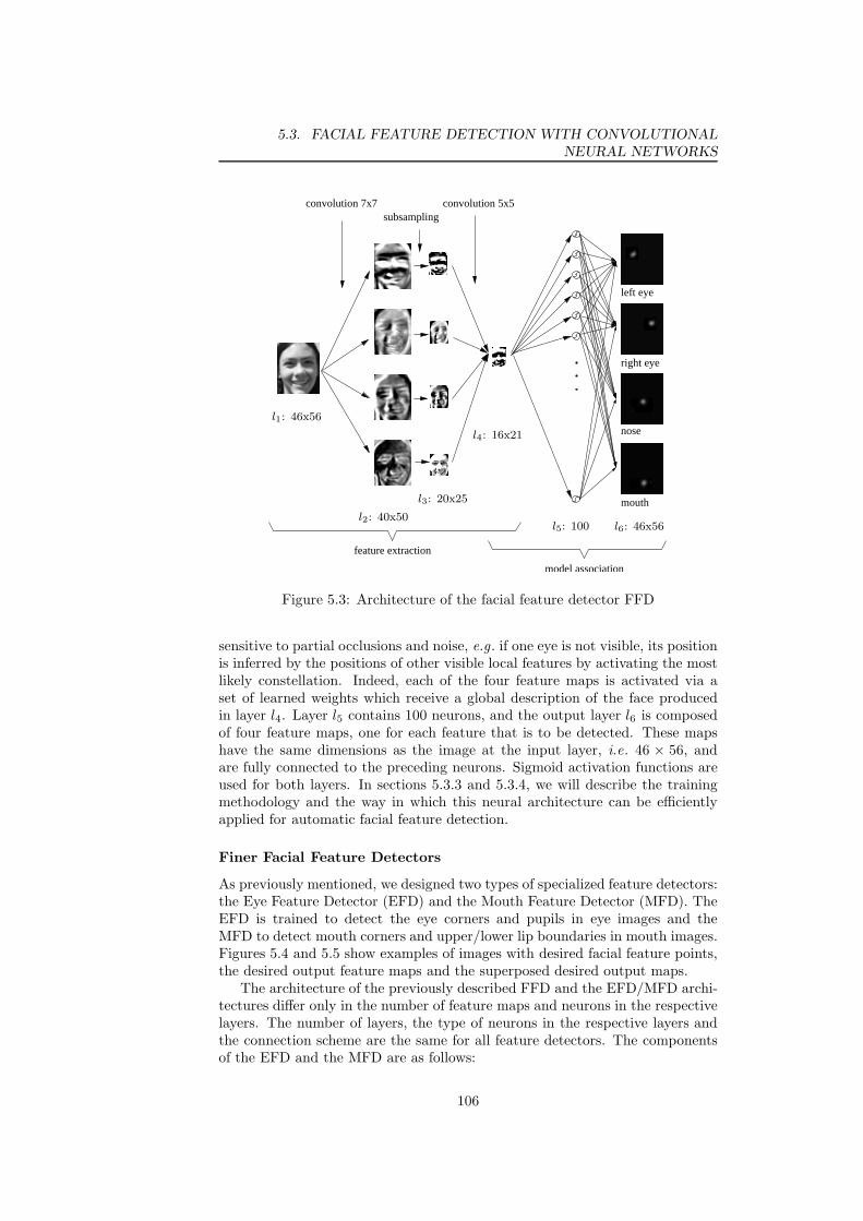
5.3. FACIAL FEATURE DETECTION WITH CONVOLUTIONAL
NEURAL NETWORKS
subsamplingconvolution 7x7 convolution 5x5
nose
left eye
right eye
mouth
feature extraction
model association
l1: 46x56
l2: 40x50
l3: 20x25
l4: 16x21
l5: 100 l6: 46x56
Figure 5.3: Architecture of the facial feature detector FFD
sensitive to partial occlusions and noise, e.g. if one eye is not visible, its positionis inferred by the positions of other visible local features by activating the mostlikely constellation. Indeed, each of the four feature maps is activated via aset of learned weights which receive a global description of the face producedin layer l4. Layer l5 contains 100 neurons, and the output layer l6 is composedof four feature maps, one for each feature that is to be detected. These mapshave the same dimensions as the image at the input layer, i.e. 46 × 56, andare fully connected to the preceding neurons. Sigmoid activation functions areused for both layers. In sections 5.3.3 and 5.3.4, we will describe the trainingmethodology and the way in which this neural architecture can be efficientlyapplied for automatic facial feature detection.
Finer Facial Feature Detectors
As previously mentioned, we designed two types of specialized feature detectors:the Eye Feature Detector (EFD) and the Mouth Feature Detector (MFD). TheEFD is trained to detect the eye corners and pupils in eye images and theMFD to detect mouth corners and upper/lower lip boundaries in mouth images.Figures 5.4 and 5.5 show examples of images with desired facial feature points,the desired output feature maps and the superposed desired output maps.
The architecture of the previously described FFD and the EFD/MFD archi-tectures differ only in the number of feature maps and neurons in the respectivelayers. The number of layers, the type of neurons in the respective layers andthe connection scheme are the same for all feature detectors. The componentsof the EFD and the MFD are as follows:
106
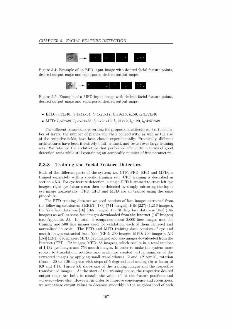
CHAPTER 5. FACIAL FEATURE DETECTION
Figure 5.4: Example of an EFD input image with desired facial feature points,desired output maps and superposed desired output maps.
Figure 5.5: Example of a MFD input image with desired facial feature points,desired output maps and superposed desired output maps.
• EFD: l1:53x40, l2:4x47x34, l3:4x23x17, l4:19x13, l5:50, l6:3x53x40
• MFD: l1:57x39, l2:5x51x33, l3:5x25x16, l4:21x12, l5:120, l6:4x57x39
The different parameters governing the proposed architectures, i.e. the num-ber of layers, the number of planes and their connectivity, as well as the sizeof the receptive fields, have been chosen experimentally. Practically, differentarchitectures have been iteratively built, trained, and tested over large trainingsets. We retained the architecture that performed efficiently in terms of gooddetection rates while still containing an acceptable number of free parameters.
5.3.3 Training the Facial Feature Detectors
Each of the different parts of the system, i.e. CFF, FFD, EFD and MFD, istrained separately with a specific training set. CFF training is described insection 4.5.3. For eye feature detection, a single EFD is trained to treat left eyeimages; right eye features can then be detected by simply mirroring the inputeye image horizontally. FFD, EFD and MFD are all trained using the sameprocedure.
The FFD training data set we used consists of face images extracted fromthe following databases: FERET [183] (744 images), PIE [227] (1,216 images),the Yale face database [16] (165 images), the Stirling face database [185] (185images) as well as some face images downloaded from the Internet (167 images)(see Appendix A). In total, it comprises about 2,000 face images used fortraining and 500 face images used for validation, each of them centered andnormalized in scale. The EFD and MFD training data consists of eye andmouth images extracted from Yale (EFD: 290 images; MFD: 290 images), AR[154] (EFD: 670 images; MFD: 375 images) and also images downloaded from theInternet (EFD: 172 images; MFD: 88 images), which results in a total numberof 1,132 eye images and 753 mouth images. In order to make the system morerobust to translation, rotation and scale, we created virtual samples of theextracted images by applying small translations (−2 and +2 pixels), rotation(from −20 to +20 degrees with steps of 5 degrees) and scaling (by a factor of0.9 and 1.1). Figure 5.6 shows one of the training images and the respectivetransformed images. At the start of the training phase, the respective desiredoutput maps are built to contain the value +1 at the feature positions and−1 everywhere else. However, in order to improve convergence and robustness,we want these output values to decrease smoothly in the neighborhood of each
107

5.3. FACIAL FEATURE DETECTION WITH CONVOLUTIONAL
NEURAL NETWORKS
Figure 5.6: Virtual face images created by applying various geometric transfor-mations
feature position. Therefore, the desired output maps are created using two-dimensional Gaussian functions centered at the feature position and normalizedbetween −1 and +1. Thus, for a particular desired feature map o having itsdesired feature at position (µx, µy), the function is as follows:
o(x, y) = 2e− 1
2
((x−µx)2
σ2x
+(y−µy)2
σ2y
)
− 1
In our experiments, we set the variances σ2x and σ2
y to 2. For illustration pur-poses, Fig. 5.2 shows an enlarged part of a desired feature map around therespective feature position.
The training phase was performed using the standard Backpropagation algo-rithm with momentum which has been adapted in order to account for weightsharing in the convolution layers l2 and l4 (see Alg. 8 on page 57). At eachiteration, every image of the training set is presented to the system and theweights are updated accordingly (online training). Classically, in order to avoidover-fitting, after each training iteration, a validation phase is performed usingthe validation set. In fact, a minimal error on the validation set is supposedto provide best generalization and the corresponding weight configuration isstored. We considered two alternative error criteria to minimize:
• the mean-squared error (MSE) between the values of the output mapsyk(i, j) and the respective values of the desired output maps ok(i, j), i.e.the error is calculated neuron by neuron:
EMSE =1
FNM
√√√√
F∑
k=1
N∑
i=1
M∑
j=1
(yk(i, j)− ok(i, j))2 , (5.1)
where F is the number of output feature maps and N×M their dimension.
• a kind of distance between the detected output feature positions (iyk, jyk)and the respective desired output feature positions (iok, jok):
Edist =1
F
√√√√
F∑
k=1
((iyk − iok)2 + (jyk − jok)2) , (5.2)
where
(iyk, jyk) = argmaxi,j
yk(i, j) and (5.3)
(iok, jok) = argmaxi,j
ok(i, j) (5.4)
108

CHAPTER 5. FACIAL FEATURE DETECTION
In our experiments, using Edist provided the best results in terms of precisionon the test sets.
5.3.4 Facial Feature Detection Procedure
Figure 5.1 illustrates the principal stages of the proposed feature detection sys-tem. In the first step, the CFF detects faces in the input image and outputs therespective face bounding boxes. The extracted faces are resized to the retinasize of the FFD and processed by the trained FFD. The eye positions, the nosetip and the mouth center in the resized face image can be inferred directly bysimply searching for the global maximum in each of the four output maps. Asthe face bounding boxes may be imprecise, the last steps are repeated for slightlytranslated and scaled face image regions. In our experiments, we achieved goodresults with translations by −4,−2, 0, +2, +4 pixels and scale factors of 0.9, 1.0and 1.1. Then, for each face image region, the sum of the maxima of the outputmaps is taken as a confidence measure, and the solution having the maximalsum is selected. Having located eye and mouth positions, the eye and mouthregions of the original image are extracted, resized and passed on to the trainedEFD and MFD. Eye and mouth features are then detected by EFD and MFDin the same way as FFD detects the four initial facial features. Finally, thedetected feature positions are mapped onto the original image.
5.3.5 Experimental Results
In order to measure the performance of the proposed facial feature detectorsystem, we first conducted several tests on FFD separately using pre-croppedface images, and later on for the whole feature detection system, i.e. CFF, FFD,EFD, MFD. To this end, we created several test sets with annotated imagesthat are neither contained in the training nor in the validation set. The testface images for FFD were extracted from PIE (1,226 images), FERET (1,058images) and from images from the Internet (384 images) (see Appendix A). Asfor the training and validation sets, the test sets were augmented with smalltransformations of the original images, i.e. translation, rotation and scaling.
The test images were presented to the feature detectors, and for each imagethe mean Euclidian distance me between the n detected feature positions andthe true feature positions, normalized with respect to the inter-ocular distancedeyes, is computed:
me =1
n deyes
n∑
k=1
√
(iyk − iok)2 + (jyk − jok)2 , (5.5)
where (iyk, jyk) is the position output by the system, and (iok, jok) is the trueposition of feature i. Over all processed images of size 46×56 pixels, deyes variesbetween 11.0 and 23.7 pixels. Thus, for example an error of 5% of the inter-ocular distance represents about 0.5 to 1.2 pixels; an error of 10% represents1.1 to 2.37 pixels. Note also that the manual feature annotation of the trainingdata can entail small errors which we neglect in these estimations.
The analysis of the performance of the FFD is presented in Figs. 5.7-5.16.Figure 5.7 shows the proportion of faces with successfully detected featuresvarying a maximum me allowed. The FERET test set clearly gave the best
109
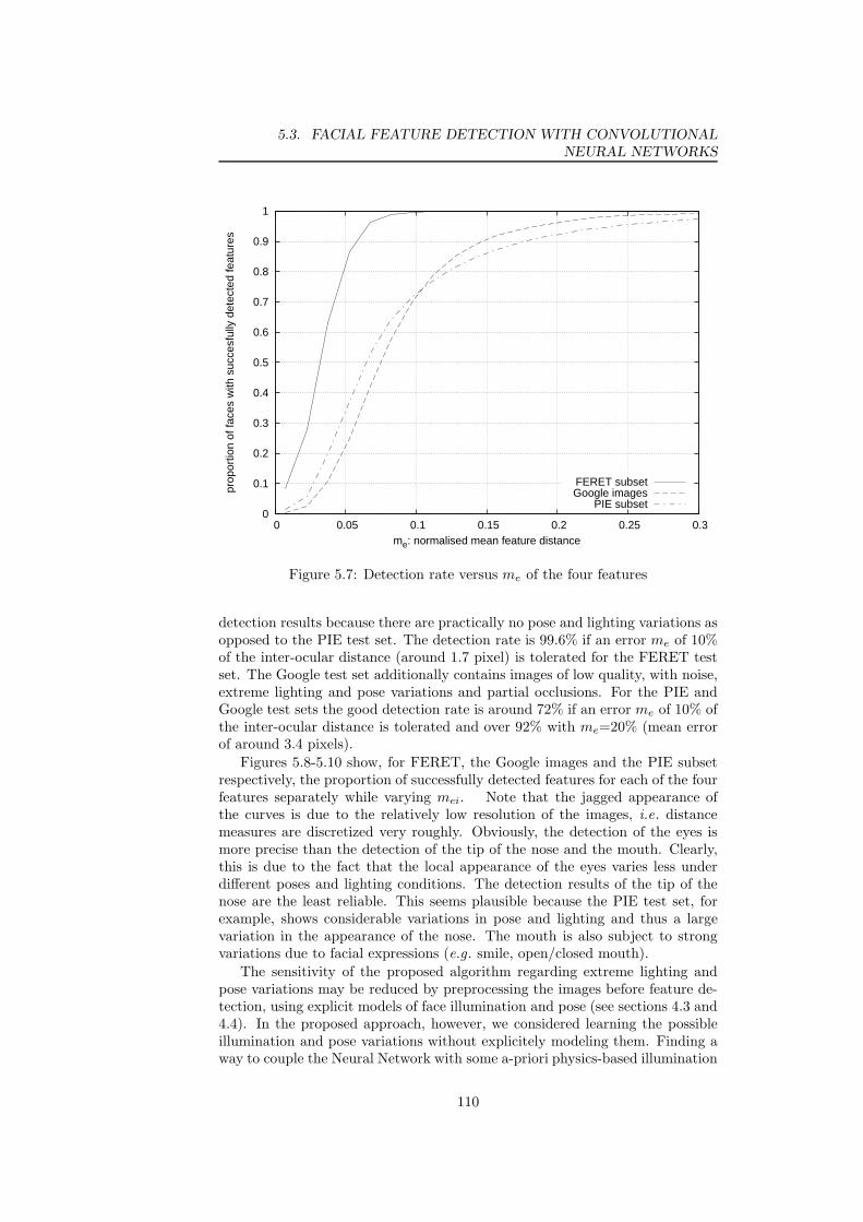
5.3. FACIAL FEATURE DETECTION WITH CONVOLUTIONAL
NEURAL NETWORKS
0
0.1
0.2
0.3
0.4
0.5
0.6
0.7
0.8
0.9
1
0 0.05 0.1 0.15 0.2 0.25 0.3
prop
ortio
n of
face
s w
ith s
ucce
sful
ly d
etec
ted
feat
ures
me: normalised mean feature distance
FERET subsetGoogle images
PIE subset
Figure 5.7: Detection rate versus me of the four features
detection results because there are practically no pose and lighting variations asopposed to the PIE test set. The detection rate is 99.6% if an error me of 10%of the inter-ocular distance (around 1.7 pixel) is tolerated for the FERET testset. The Google test set additionally contains images of low quality, with noise,extreme lighting and pose variations and partial occlusions. For the PIE andGoogle test sets the good detection rate is around 72% if an error me of 10% ofthe inter-ocular distance is tolerated and over 92% with me=20% (mean errorof around 3.4 pixels).
Figures 5.8-5.10 show, for FERET, the Google images and the PIE subsetrespectively, the proportion of successfully detected features for each of the fourfeatures separately while varying mei. Note that the jagged appearance ofthe curves is due to the relatively low resolution of the images, i.e. distancemeasures are discretized very roughly. Obviously, the detection of the eyes ismore precise than the detection of the tip of the nose and the mouth. Clearly,this is due to the fact that the local appearance of the eyes varies less underdifferent poses and lighting conditions. The detection results of the tip of thenose are the least reliable. This seems plausible because the PIE test set, forexample, shows considerable variations in pose and lighting and thus a largevariation in the appearance of the nose. The mouth is also subject to strongvariations due to facial expressions (e.g. smile, open/closed mouth).
The sensitivity of the proposed algorithm regarding extreme lighting andpose variations may be reduced by preprocessing the images before feature de-tection, using explicit models of face illumination and pose (see sections 4.3 and4.4). In the proposed approach, however, we considered learning the possibleillumination and pose variations without explicitely modeling them. Finding away to couple the Neural Network with some a-priori physics-based illumination
110

CHAPTER 5. FACIAL FEATURE DETECTION
0
0.2
0.4
0.6
0.8
1
0 0.05 0.1 0.15 0.2 0.25 0.3
prop
ortio
n of
suc
cesf
ully
det
ecte
d fe
atur
es
mei: normalised feature distance
left eyeright eye
mouthnose
Figure 5.8: Detection rate versus mei of each facial feature (FERET)
0
0.1
0.2
0.3
0.4
0.5
0.6
0.7
0.8
0.9
1
0 0.05 0.1 0.15 0.2 0.25 0.3
prop
ortio
n of
suc
cesf
ully
det
ecte
d fe
atur
es
mei: normalised feature distance
left eyeright eye
mouthnose
Figure 5.9: Detection rate versus mei of each facial feature (Google images)
111

5.3. FACIAL FEATURE DETECTION WITH CONVOLUTIONAL
NEURAL NETWORKS
0
0.1
0.2
0.3
0.4
0.5
0.6
0.7
0.8
0.9
1
0 0.05 0.1 0.15 0.2 0.25 0.3
prop
ortio
n of
suc
cesf
ully
det
ecte
d fe
atur
es
mei: normalised feature distance
left eyeright eye
mouthnose
Figure 5.10: Detection rate versus mei of each facial feature (PIE subset)
models may reduce the degrees of freedom of the model and help classification.This is an issue which is not treated in this work but might be an interestingidea to explore in the future.
So far, we simply used the normalized pixel intensities, i.e. the raw images,as the CNN input. Figure 5.11(a) shows one example image. It is however notobvious that this is the optimal choice of input features. For that reason, we alsotrained two other CNNs with the same training data but receiving pre-processedface images at their input layer. The first alternative is to use gradient images.In this case, the input images are processed with a horizontal and a verticalSobel filter resulting in two gradient images. Thus, the input layer now containstwo input maps fully connected to the first convolution layer. Figure 5.11(b)illustrates the respective filtered results of the image shown in 5.11(a). Thesecond alternative is to process the input face image with Gabor wavelet filtersof selected scales and orientations. Gabor wavelets are hierarchically arranged,Gaussian modulated sinusoids. There is evidence that this is the way imagesare processed in the primary visual cortex (V1) of the human brain [150]. Wechose three different scales and four orientations resulting in 12 Gabor wavelets.Figure 5.11(c) shows the resulting outputs of the respective wavelet filters forthe image in Fig. 5.11(a). Note that in any case the input images are normalizedto be in the range [−1, +1] before presenting them to the CNN.
We trained two distinct CNNs with the same training data as the previouslydescribed FFD system (see section 5.3.3), i.e. for the task of detecting fourfeature points. The architecture of the two CNNs was almost the same as theone depicted in Fig. 5.3. The only difference was the number of inputs dependingon the type of features used, i.e. two input maps for gradient images and 12maps for the Gabor wavelet filter responses.
112

CHAPTER 5. FACIAL FEATURE DETECTION
(a) Raw input image
(b) Gradient images
(c) Gabor wavelet filter responses
Figure 5.11: The different types of input features that have been tested
Figures 5.12-5.14 compare the precision of the three trained CNNs by meansof the ROC curves on the FERET database, the Google images and the PIE sub-set respectively. The ROC curves clearly show that on all tested databases theCNN trained with the raw input images, i.e. only image intensities, outperformsthose trained with gradient images and Gabor wavelet filter responses. Theseresults suggest that CNNs trained for this type of face analysis task somehowmake use of the information contained in the absolute image intensities whichis largely or completely suppressed by using gradients or Gabor wavelet filters.
Another negative side-effect of using gradient images and especially Gaborwavelet filtered input images is the higher number of connections and thustrainable parameters of the CNN. This increase in complexity not only entails ahigher risk of overfitting the data but also a much slower learning and processingtime of the CNN in addition to the time spent for filtering the input images.Finally, when using Gabor wavelets one has to “manually” choose appropriatescales and orientations of the respective filters for a given problem, which is nota trivial task. Hence, for the rest of this work, we only use the raw images asthe input for the CNNs.
Let us now analyze the sensitivity of the proposed feature detection systemwith respect to pixel noise and partial occlusions. To this end, we conducted twoexperiments on the FERET test set, the PIE subset and the Google images. Inthe first experiment, we added Gaussian noise with varying standard deviation σto each pixel of the normalized face images (being in the range [0..255]). Figure5.15 shows the mean feature error me with σ varying from 0 to 70. Note thatthe proposed feature detector is very robust to noise as the error me remainsrather low while adding a considerable amount of noise. For the worst of thethree test sets (PIE subset) me stays below 20% for σ = 50. Example imageswith corresponding amounts of added noises are shown at the top of Fig. 5.15.
The second experiment consists in occluding a certain percentage of the faceimages by a black zone in the lower part. Figure 5.16 shows the mean featureerror me with an occlusion from 0 to 50%. For occlusions smaller than 40%the only invisible feature, in most of the cases, is the mouth, and the error me
remains almost constant. Larger occlusions cover both mouth and nose, whichexplains the abrupt increase of me in all of the three test sets.
113

5.3. FACIAL FEATURE DETECTION WITH CONVOLUTIONAL
NEURAL NETWORKS
0
0.1
0.2
0.3
0.4
0.5
0.6
0.7
0.8
0.9
1
0 0.05 0.1 0.15 0.2 0.25 0.3
pro
port
ion o
f fa
ces w
ith s
uccessfu
lly d
ete
cte
d featu
res
me: normalized mean feature distance
Image intensitiesGradients
Gabor wavelet filter responses
Figure 5.12: ROC curves comparing the CNNs trained with different inputfeatures (FERET database)
0
0.1
0.2
0.3
0.4
0.5
0.6
0.7
0.8
0.9
1
0 0.05 0.1 0.15 0.2 0.25 0.3
pro
port
ion o
f fa
ces w
ith s
uccessfu
lly d
ete
cte
d featu
res
me: normalized mean feature distance
Image intensitiesGradients
Gabor wavelet filter responses
Figure 5.13: ROC curves comparing the CNNs trained with different inputfeatures (Google images)
114
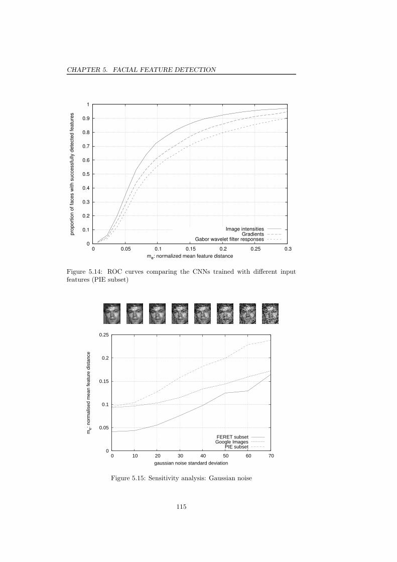
CHAPTER 5. FACIAL FEATURE DETECTION
0
0.1
0.2
0.3
0.4
0.5
0.6
0.7
0.8
0.9
1
0 0.05 0.1 0.15 0.2 0.25 0.3
pro
port
ion o
f fa
ces w
ith s
uccessfu
lly d
ete
cte
d featu
res
me: normalized mean feature distance
Image intensitiesGradients
Gabor wavelet filter responses
Figure 5.14: ROC curves comparing the CNNs trained with different inputfeatures (PIE subset)
0
0.05
0.1
0.15
0.2
0.25
0 10 20 30 40 50 60 70
me:
nor
mal
ised
mea
n fe
atur
e di
stan
ce
gaussian noise standard deviation
FERET subsetGoogle Images
PIE subset
Figure 5.15: Sensitivity analysis: Gaussian noise
115
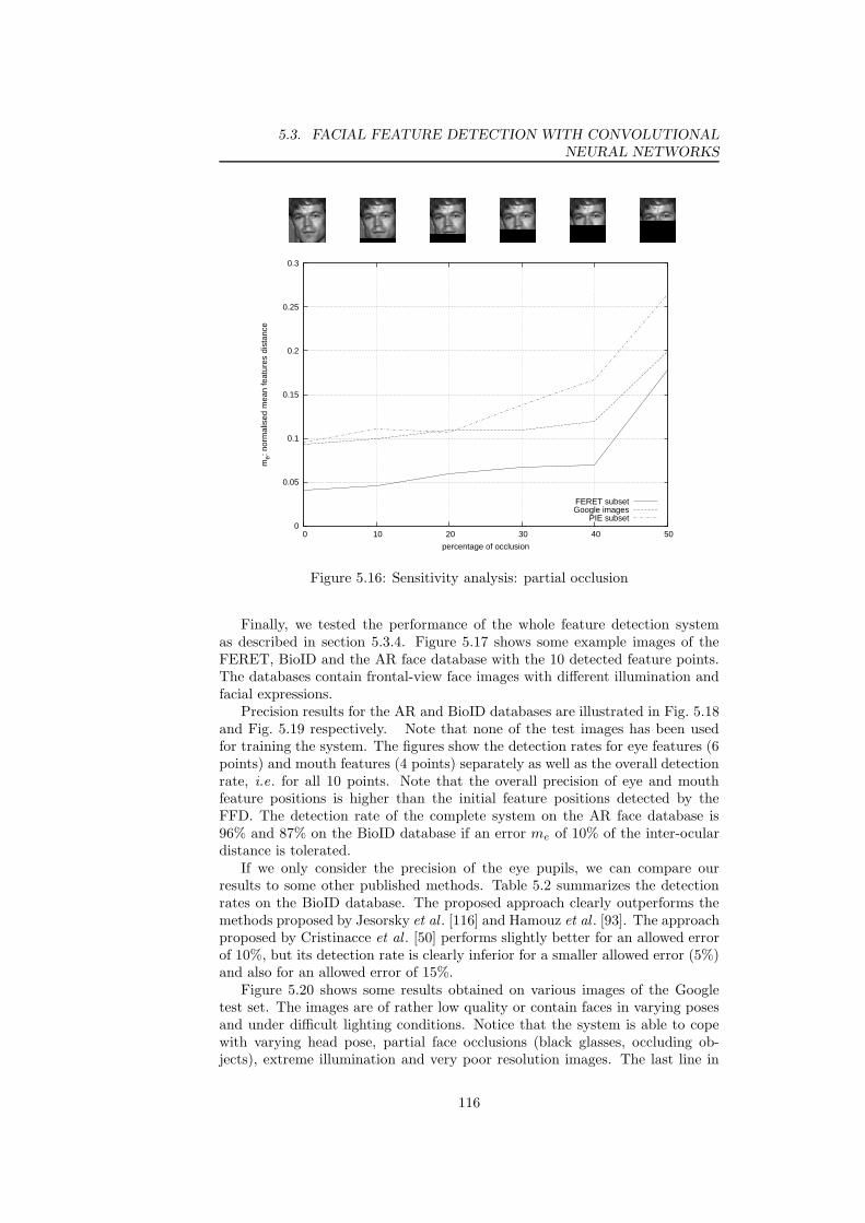
5.3. FACIAL FEATURE DETECTION WITH CONVOLUTIONAL
NEURAL NETWORKS
0
0.05
0.1
0.15
0.2
0.25
0.3
0 10 20 30 40 50
me:
nor
mal
ised
mea
n fe
atur
es d
ista
nce
percentage of occlusion
FERET subsetGoogle images
PIE subset
Figure 5.16: Sensitivity analysis: partial occlusion
Finally, we tested the performance of the whole feature detection systemas described in section 5.3.4. Figure 5.17 shows some example images of theFERET, BioID and the AR face database with the 10 detected feature points.The databases contain frontal-view face images with different illumination andfacial expressions.
Precision results for the AR and BioID databases are illustrated in Fig. 5.18and Fig. 5.19 respectively. Note that none of the test images has been usedfor training the system. The figures show the detection rates for eye features (6points) and mouth features (4 points) separately as well as the overall detectionrate, i.e. for all 10 points. Note that the overall precision of eye and mouthfeature positions is higher than the initial feature positions detected by theFFD. The detection rate of the complete system on the AR face database is96% and 87% on the BioID database if an error me of 10% of the inter-oculardistance is tolerated.
If we only consider the precision of the eye pupils, we can compare ourresults to some other published methods. Table 5.2 summarizes the detectionrates on the BioID database. The proposed approach clearly outperforms themethods proposed by Jesorsky et al . [116] and Hamouz et al . [93]. The approachproposed by Cristinacce et al . [50] performs slightly better for an allowed errorof 10%, but its detection rate is clearly inferior for a smaller allowed error (5%)and also for an allowed error of 15%.
Figure 5.20 shows some results obtained on various images of the Googletest set. The images are of rather low quality or contain faces in varying posesand under difficult lighting conditions. Notice that the system is able to copewith varying head pose, partial face occlusions (black glasses, occluding ob-jects), extreme illumination and very poor resolution images. The last line in
116

CHAPTER 5. FACIAL FEATURE DETECTION
Figure 5.17: Facial feature detection results on different face databases: top:FERET, middle: BioID, bottom: AR face database
0
0.1
0.2
0.3
0.4
0.5
0.6
0.7
0.8
0.9
1
0 0.05 0.1 0.15 0.2 0.25 0.3 0.35 0.4 0.45 0.5
prop
ortio
n of
imag
es w
ith s
ucce
sful
ly d
etec
ted
feat
ures
me: normalised mean feature distance
eyes (6 points)mouths (4 points)
all (10 points)
Figure 5.18: Overall detection rate for AR
117

5.3. FACIAL FEATURE DETECTION WITH CONVOLUTIONAL
NEURAL NETWORKS
0
0.1
0.2
0.3
0.4
0.5
0.6
0.7
0.8
0.9
1
0 0.05 0.1 0.15 0.2 0.25 0.3 0.35 0.4 0.45 0.5
prop
ortio
n of
imag
es w
ith s
ucce
sful
ly d
etec
ted
feat
ures
me: normalised mean feature distance
eyes (6 points)mouths (4 points)
all (10 points)
Figure 5.19: Overall detection rate for BioID
Allowed error w.r.t. deyes
Method 5% 10% 15%
Jesorsky et al . [116] 40% 79% 93%Cristinacce et al . [50] 60% 96% 97%Hamouz et al . [93] 50% 66% 70%
proposed approach 79% 92% 98%
Table 5.2: Comparison of eye pupil detection rates of some published methodson the BioID database
118

CHAPTER 5. FACIAL FEATURE DETECTION
Figure 5.20: Some results of combined face and facial feature detection
119
5.4. CONCLUSION
Fig. 5.20 contains some images with imprecisely detected features. Naturally,the precision drops with this test set but we still obtained a detection rate of76% with an allowed error of 10% and 92% with an allowed error of 15% of theinter-ocular distance.
The FFD detecting four facial feature points has also been implemented onembedded platforms by Roux et al . [204]. A considerable gain in speed of thealgorithm has been obtained by the authors by reducing the memory usage andconducting further algorithmic optimizations. The final version processed 68.7faces/s on a Pentium IV at 3.2 GHz and 12.8 faces/s on a Xscale PXA27x at624 MHz. For an application with integrated face and facial feature detectoron a Xscale PXA27x, they further report an execution time of 7 frames/s forQCIF images (176× 144 pixels) containing one face per image.
5.4 Conclusion
In this chapter, we presented the problem of facial feature detection in images,which is considered a key issue in many facial analysis applications. We firstoutlined the state-of-the-art in this field and then proposed a novel approachto facial feature detection using Convolutional Neural Networks (CNN). Thesystem is composed of several CNNs having a specific architecture and operatingon different levels in a hierarchical manner. The first level CNN which we calledFFD detects four facial features: the eyes, the nose tip and the mouth centerand then extracts the regions around the eyes and the mouth and passes themon to specialized feature detectors, the so-called Eye Feature Detector (EFD)and the Mouth Feature Detector (MFD), which in turn detect 10 more specificfacial features such as the eye or mouth corners.
Each of the single feature detectors is trained with a set of face, eye or mouthimages annotated with the respective feature positions.
Our experimental results show that using the image intensities as input of theCNN yields to the best results compared to gradient images and Gabor waveletfilter responses. We then presented the detection rates on different public andprivate face databases and experimentally show that the proposed approachis precise and very robust to pixel noise and partial occlusions. Further, thesystem shows to be insensitive to extreme lighting conditions and varying pose.Comparing the precision results of eye pupil detection on the BioID database,the proposed approach outperforms other state-of-the-art systems.
120
Chapter 6
Face and Gender
Recognition
6.1 Introduction
Automatic face recognition is a central topic in face analysis-related research,and it has gained a lot of importance during the last decades due to the vast num-ber of possible applications (see section 1.2). Let us recall that one can differ-entiate two types of applications: open-world and closed-world. A closed-worldface recognition system only copes with a limited number of known personswhereas an open-world application also implements the notion of an unknownperson, corresponding to all persons that have not been explicitely learned bythe system. Moreover, as already mentioned in section 1.2, face recognitioncan be employed for authentication or verification purposes. That means, givenan input face image, a face authentication system is supposed to reply with theidentity of the respective person, whereas a face verification system additionallyreceives a claimed identity and decides if this identity corresponds to the faceor not. In any case, both of these applications are classification problems, and,from a technical point of view, they differ only marginally.
In this chapter, we will briefly describe some of the most important ap-proaches to automatic face recognition. We will then propose a novel facerecognition method based on image reconstruction using Convolutional NeuralNetworks. Further, we present experimental results showing the effectiveness ofthis approach and its robustness to noise and partial occlusions.
Finally, we will turn to the problem of gender recognition which is similar toface recognition in that it is also a classification problem. However, in this case,there are only two classes: male and female. We propose a CNN-based approachwith a topology similar to the Convolutional Face Finder (CFF) described insection 4.2.3. We then experimentally show that, in terms of classification rate,this classifier achieves comparable results to previously published gender recog-nition methods based on Adaboost and SVMs.
121

6.2. STATE-OF-THE-ART IN FACE RECOGNITION
6.2 State-of-the-art in Face Recognition
There are numerous works in the field of automatic face recognition and thenumber of publications has been constantly increasing in the last years (seeGross et al . [90] and Zhao and Chellappa [272] for literature surveys). Theexisting approaches can be roughly divided into two groups: global and localapproaches of which the most important ones will be outlined in the following.Note that the majority of face recognition methods require the face to be local-ized in the input image beforehand. Some even necessitate a precise alignmentof the face, such that it is in an upright position, centered and in a predefinedscale.
Global Approaches
Global approaches process the face image as a whole mostly applying some typeof statistical projection. The idea is to form a one-dimensional vector from theinput image and project this (high-dimensional) vector into a sub-space of lowerdimension where classification is supposed to be easier. Thus, such a projection– mostly linear – is supposed to select the most prominent features in order todiscriminate the faces of different persons.
The most well-known of these approaches is the so-called Eigenfaces methodintroduced by Turk and Pentland [243]. Here, a PCA (c.f . section 2.2.1) is per-formed on the set of training face images projecting them into a linear subspacewhere the orthogonal eigen-vectors represent best the distribution of face vec-tors. The classification of new face images is then performed by projectingthem into the linear subspace, forming a vector by selecting the eigen-valuesof the most discriminant dimensions and comparing these vectors to the onesof the training images. Much work has been done on the choice of the eigen-vectors. For example, Kirby and Sirovich [122] proposed a criterion based ona so-called energy dimension (see section 2.2.1) where the dimensions with thelargest eigen-values are kept such that the normalized sum of these eigen-valuesis beyond a certain threshold (e.g. 90%). Martinez et al . [155] showed thatthe recognition rate can be improved by ignoring the first three dimensions,commonly deemed to account for illumination changes.
Another well-known approach presented by Belhumeur et al . [16] uses theLinear Discriminant Analysis (LDA) (c.f . section 2.2.2) and is called Fisher-faces as it maximizes the Fisher’s criterion, i.e. a quotient of inter-class andintra-class variance. This means, it is not concerned with the best represen-tation of the input data but rather with its maximum separability. However,since the dimension of the input vectors (the face images) is much greater thantheir number, there is a singularity problem when inverting the matrix of intra-class variance. To avoid this a PCA on the input vectors can be performedbeforehand.
Numerous variants of these linear projection methods have been proposedin the literature [205, 236, 165, 233, 271]. Algorithms based on the IndependentComponent Analysis (ICA) have also been presented by Bartlett et al . [12].
More recently, Visani et al . [253] introduced an approach based on the Bilin-ear Discriminant Analysis (BDA) which realizes a two-dimensional linear pro-jection of the lines and the columns of the face images. Then, they appliedNormalized Radial Basis Function Networks to classify the projected vectors.
122
CHAPTER 6. FACE AND GENDER RECOGNITION
A technique called Discriminative Common Vectors (DCV) is due to Cevi-kalp et al . [36], which is a variation of the LDA for small sample sizes. For eachindividual they calculated a so-called common vector which is the result of aprojection that eliminates features corresponding to the respective intra-classvariation. Then, classification was performed using the common vectors.
There are also some approaches that do not use only one vector subspacebut several. For example, the approach by Pentland et al . [181] computes asubspace for each orientation and scale of a face in the input image. A new faceis then recognized by projecting the image into all subspaces and selecting theone where it is the closest to an vector of the face database.
Vasilescu et al . [247] have generalized this technique by using tensors. Intheir approach they proposed four-dimensional tensors corresponding to class,pose, illumination condition and facial expression respectively.
Other projection approaches [242, 262, 237, 261] construct a separate sub-space for each class, i.e. each person.
A different face recognition approach has been introduced by Cootes et al .[41] called Active Appearance Models (AAM). As outlined in section 5.2, thismethod models independently shape and texture of the face by applying PCArespectively. The vector of shape and texture coefficients is then used for recog-nition. Thus, a new face that is to be recognized is fit to the model by aniterative optimization procedure and the resulting shape and texture parame-ters are compared to the ones from the training database. Lanitis et al . [131]applied this method for the first time to face recognition. Also, Edwards et al .[60] and Kumar et al . [128] presented face recognition methods based on AAMs.
Neural Networks have also been applied to automatic face recognition. Forexample, Lawrence et al . [132] proposed a method based on Self-OrganizingMaps (SOM) to cluster the set of training images and thus construct a lower-dimensional subspace that conserves the topology of the input space. Afterprojecting a face image onto the SOM, they applied a Convolutional NeuralNetwork (CNN) in order to classify the signatures, i.e. the low-dimensionalvectors.
Cottrell and Fleming [45] proposed to extract features by a non-linear pro-jection using an Auto-Associative Neural Network (AANN). To classify the re-sulting features the applied a trained Multi-Layer Perceptron (MLP).
The approach of Lin et al . [146] uses probabilistic decision-based NeuralNetworks combining the advantages of statistical approaches and Neural Net-works. Further, there are many approaches using Radial Basis Function Net-works (RBFN) to classify feature vectors previously extracted, for example by alinear projection. Thomaz et al . [235] and Er et al . [62] proposed such methods.
Support Vector Machines (SVM), introduced by Vapnik [246], have alsobeen used in the context of face recognition. Philips [184], for example, firstused Bayesian subspaces to reduce the problem to two classes: inter-class andintra-class variations. Then, SVMs were applied for classification.
Finally, Jonsson et al . [119] presented a face authentication method usingone SVM per person in order to classify the signatures obtained by PCA or byLDA.
123

6.2. STATE-OF-THE-ART IN FACE RECOGNITION
Local Approaches
Local face recognition approaches rely on a separate processing of different re-gions in a face image. Mostly, this implies the extraction of local facial features.Often, local and global processing is combined in order to put the different localfeatures into relation with each other. The most important of them are outlinedin the following.
Brunelli and Poggio [33] proposed a technique that automatically extractsa set of 30 geometrical features from face images. In order to recognize a face,they compared these features pairwise using a Mahalanobis distance.
Another geometric approach has been proposed by Takacs [234] who usedbinary contour maps extracted from the face images by a Sobel filter. Thesimilarity between two contours was then computed by using a variant of theHausdorff distance. This approach has been extended by Gao et al . [80] bytransforming the contour maps into so-called Line Edge Maps (LEM) containinga list of line segments. The distance measure, however, was the same as the oneTakacs used.
Pentland et al . [181] introduced the approach of “Modular Eigenspaces”performing a PCA and classification on separate facial regions, i.e. the eyes,the nose and the overall face image. The mouth region showing much variationdue to facial expressions leaded to a decrease of the recognition rate in theirexperiments.
The approach due to Heisele et al . [96] first detects the face region and10 facial feature points using their previously published face and facial featuredetector [97]. Then, the image regions around the respective facial features areextracted. Finally, the concatenated line (or row) vectors of these regions werecombined to one large vector that is classified by a SVM.
Face regions were also extracted by a method proposed by Price and Gee[189]. Here, the authors considered three different image regions: a rectangularband going from the forehead to the bottom of the nose, one containing the twoeyes and one being the entire image itself. Finally, they applied a variant ofLDA to classify the respective face regions.
Another approach called Local Component Analysis (LCA) is due to Penevand Atick [180]. They performed several PCAs to extract different local featuresand combined them in a sort of deformable grid. A procedure that minimizesthe reconstruction error finds then the optimal set of local grids.
Samaria et al . [214] introduced an approach based on Hidden Markov Models(HMM). Here, the face images were segmented into a certain number of over-lapping sub-bands, and these sub-bands were in turn concatenated to a largeone-dimensional vector or compressed by DCT. Then for each class, i.e. eachperson, a HMM was created reflecting the probabilistic sequence of sub-bands.New face images were classified applying the well-known Viterbi algorithm inorder to compare the sequence of respective sub-bands with the trained models.
This approach has also been extended to so-called pseudo-2D HMMs [214,169] which model horizontal and vertical sequences of image blocks. However,the blocks are not completely connected to each other, hence the approach iscalled pseudo-2D (see section 2.4.4).
Perronnin et al . [182] proposed an approach based on a 2D HMM frame-work where facial expressions and illumination variations were independentlymodeled. In this framework, a grid is placed on the face image where at each
124
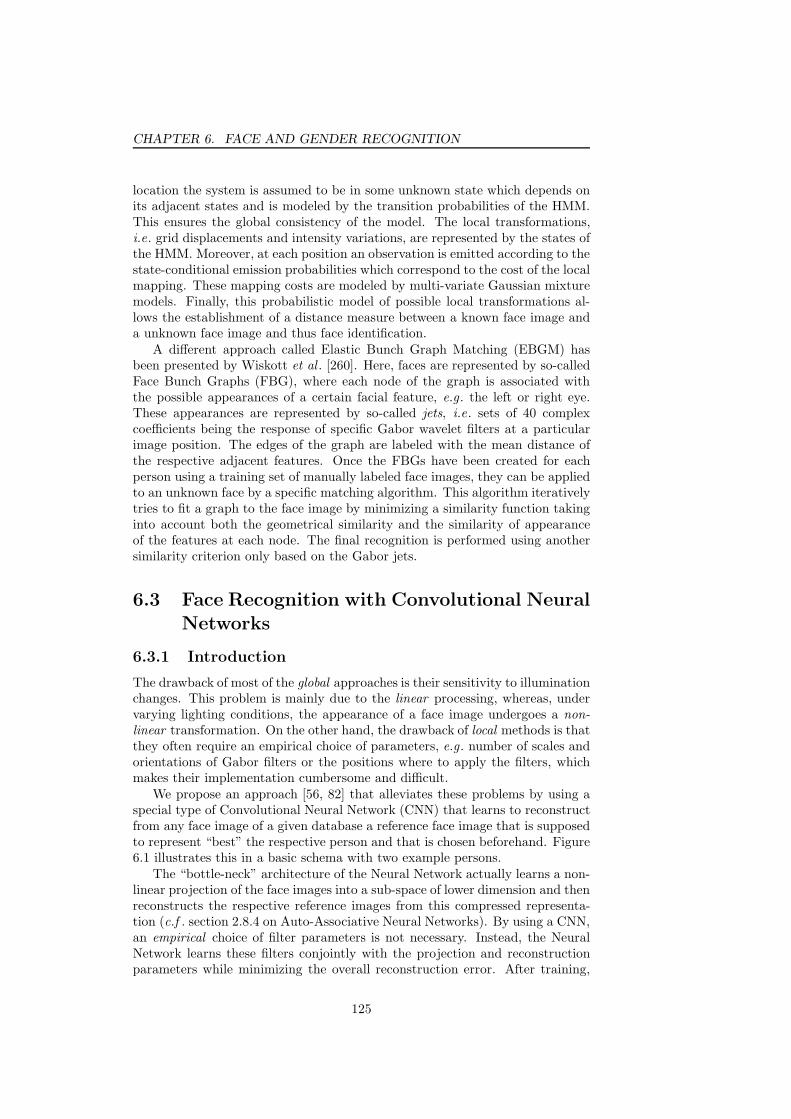
CHAPTER 6. FACE AND GENDER RECOGNITION
location the system is assumed to be in some unknown state which depends onits adjacent states and is modeled by the transition probabilities of the HMM.This ensures the global consistency of the model. The local transformations,i.e. grid displacements and intensity variations, are represented by the states ofthe HMM. Moreover, at each position an observation is emitted according to thestate-conditional emission probabilities which correspond to the cost of the localmapping. These mapping costs are modeled by multi-variate Gaussian mixturemodels. Finally, this probabilistic model of possible local transformations al-lows the establishment of a distance measure between a known face image anda unknown face image and thus face identification.
A different approach called Elastic Bunch Graph Matching (EBGM) hasbeen presented by Wiskott et al . [260]. Here, faces are represented by so-calledFace Bunch Graphs (FBG), where each node of the graph is associated withthe possible appearances of a certain facial feature, e.g. the left or right eye.These appearances are represented by so-called jets, i.e. sets of 40 complexcoefficients being the response of specific Gabor wavelet filters at a particularimage position. The edges of the graph are labeled with the mean distance ofthe respective adjacent features. Once the FBGs have been created for eachperson using a training set of manually labeled face images, they can be appliedto an unknown face by a specific matching algorithm. This algorithm iterativelytries to fit a graph to the face image by minimizing a similarity function takinginto account both the geometrical similarity and the similarity of appearanceof the features at each node. The final recognition is performed using anothersimilarity criterion only based on the Gabor jets.
6.3 Face Recognition with Convolutional Neural
Networks
6.3.1 Introduction
The drawback of most of the global approaches is their sensitivity to illuminationchanges. This problem is mainly due to the linear processing, whereas, undervarying lighting conditions, the appearance of a face image undergoes a non-linear transformation. On the other hand, the drawback of local methods is thatthey often require an empirical choice of parameters, e.g. number of scales andorientations of Gabor filters or the positions where to apply the filters, whichmakes their implementation cumbersome and difficult.
We propose an approach [56, 82] that alleviates these problems by using aspecial type of Convolutional Neural Network (CNN) that learns to reconstructfrom any face image of a given database a reference face image that is supposedto represent “best” the respective person and that is chosen beforehand. Figure6.1 illustrates this in a basic schema with two example persons.
The “bottle-neck” architecture of the Neural Network actually learns a non-linear projection of the face images into a sub-space of lower dimension and thenreconstructs the respective reference images from this compressed representa-tion (c.f . section 2.8.4 on Auto-Associative Neural Networks). By using a CNN,an empirical choice of filter parameters is not necessary. Instead, the NeuralNetwork learns these filters conjointly with the projection and reconstructionparameters while minimizing the overall reconstruction error. After training,
125

6.3. FACE RECOGNITION WITH CONVOLUTIONAL NEURAL
NETWORKS
Reconstruction
Projection
Reconstruction
Projection
reference imageperson 1
reference imageperson 2
Person 1
Person 2
projected vectors
projected vectors
Figure 6.1: The basic schema of our approach showing two different individuals
face images can be classified by calculating distances between the respectiveprojected vectors in the intermediate layer of the network or the distances be-tween the respective reconstructed images at the output of the network.
6.3.2 Neural Network Architecture
The proposed neural architecture is a specific type of CNN consisting of sixlayers, where the first layer is the input layer, the three following layers areconvolutional and sub-sampling layers, and the last two layers are standardfeed-forward neuron layers. For details on CNNs, we refer to chapter 3 andin particular section 3.2.2. Our system is trained to transform an input faceimage into a reference image which is automatically chosen for each person torecognize. Figure 6.2 gives an overview of the architecture.
The retina l1 receives a cropped face image of 46 × 56 pixels, containinggray values normalized between −1 and +1. The second layer l2 consists of fourfeature maps which are all connected to the input map and which perform aconvolution with a trainable 7×7 kernel followed by a linear activation function.The third layer l3 sub-samples its input feature maps by a factor of two and usesa sigmoid activation function. Layer l4 is another convolutional layer with 5×5kernels. It contains three feature maps, each connected to two preceding mapsas illustrated in figure 6.2. By combining the results of the low-level featuredetectors, like edges or corners, it extracts higher-level features correspondingto more characteristic forms or patterns of a face image. Unlike the secondlayer, a sigmoid activation function is used here.
While the previous layers act principally as local feature extraction layers,
126
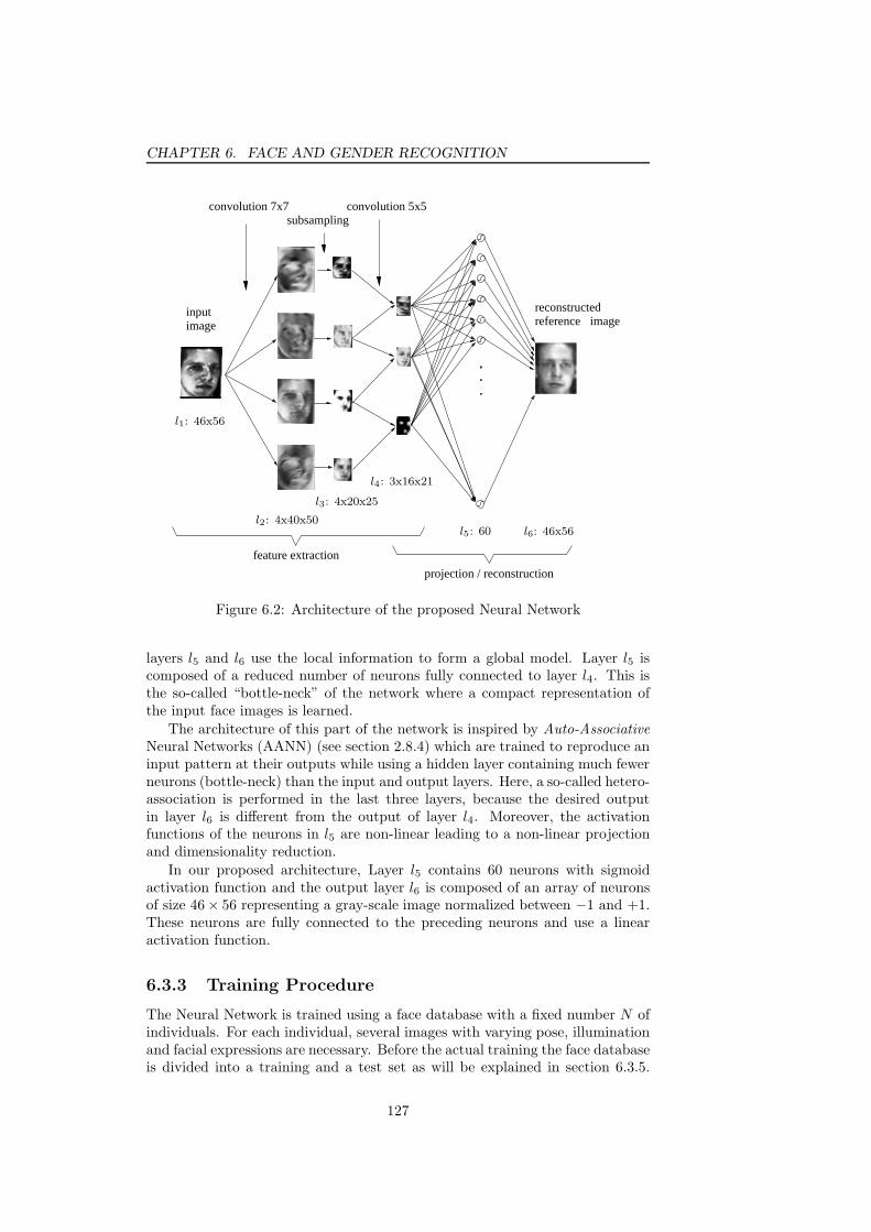
CHAPTER 6. FACE AND GENDER RECOGNITION
inputimage
reconstructedreference image
subsamplingconvolution 7x7 convolution 5x5
feature extraction
projection / reconstruction
l1: 46x56
l2: 4x40x50
l3: 4x20x25
l4: 3x16x21
l5: 60 l6: 46x56
Figure 6.2: Architecture of the proposed Neural Network
layers l5 and l6 use the local information to form a global model. Layer l5 iscomposed of a reduced number of neurons fully connected to layer l4. This isthe so-called “bottle-neck” of the network where a compact representation ofthe input face images is learned.
The architecture of this part of the network is inspired by Auto-AssociativeNeural Networks (AANN) (see section 2.8.4) which are trained to reproduce aninput pattern at their outputs while using a hidden layer containing much fewerneurons (bottle-neck) than the input and output layers. Here, a so-called hetero-association is performed in the last three layers, because the desired outputin layer l6 is different from the output of layer l4. Moreover, the activationfunctions of the neurons in l5 are non-linear leading to a non-linear projectionand dimensionality reduction.
In our proposed architecture, Layer l5 contains 60 neurons with sigmoidactivation function and the output layer l6 is composed of an array of neuronsof size 46× 56 representing a gray-scale image normalized between −1 and +1.These neurons are fully connected to the preceding neurons and use a linearactivation function.
6.3.3 Training Procedure
The Neural Network is trained using a face database with a fixed number N ofindividuals. For each individual, several images with varying pose, illuminationand facial expressions are necessary. Before the actual training the face databaseis divided into a training and a test set as will be explained in section 6.3.5.
127

6.3. FACE RECOGNITION WITH CONVOLUTIONAL NEURAL
NETWORKS
The training procedure consists of two successive steps:
1. selection of the reference images and
2. actual training of the Neural Network.
These steps are detailed in the following.
Choosing the Reference Images
Let us denote imij the j-th example image of individual i = 1..N in the facedatabase (j = 1..Mi). For each individual i a reference image ri among theface images imij in the training set has to be chosen. The Neural Network isthen trained to respond for any input image imij of a given individual withthe respective reference image ri for that individual. In this way, it will learnto extract features invariant to the intra-class variations present in the trainingimages, e.g. pose, illumination or facial expressions.
We experimented with two different strategies for choosing the referenceimages. They are both based on a Euclidean distance measure between therespective image vectors im+
ij , defined as the one-dimensional vectors obtainedby concatenating the rows of the respective images imij . The strategies weinvestigated are the following:
1. Choose the most representative image:
The face image of the individual i that is closest to the mean image im+i
of i is chosen:
ri = argminim
+ij
‖im+ij − im+
i ‖ ∀ i ∈ 1..N, j ∈ 1..Mi . (6.1)
2. Choose the most distant image:The face image of the individual i that has the greatest distance to theface images of all the other individuals is chosen.
ri = argmaxim
+ij
‖im+ij − im
+kl‖
∀ i, k ∈ 1..N, j ∈ 1..Mi, l ∈ 1..Mk, k 6= i . (6.2)
We will call these strategies MEAN and DIST in the following.
Training the Neural Network
In order to construct the training set for the Neural Network the face imagesare normalized in the following way. First, each image is cropped in such away that the face is centered and that the eyes and the mouth are roughlyat predefined positions while keeping the aspect ratio. Then, each image ishistogram-equalized and resized to the dimensions of the retina l1 (46 × 56).Training is performed using the Backpropagation algorithm which has beenslightly adapted to account for the shared weights in layers l2 to l4 (see Alg. 8on page 57). For a given example imij the objective function is the following:
Ei =1
WH
WX
x=1
HX
y=1
(di(x, y) − y6(x, y))2 , (6.3)
128
CHAPTER 6. FACE AND GENDER RECOGNITION
which is the mean squared error (MSE) between the computed outputs y6(x, y)for training example imij and the desired outputs di(x, y), where di representsthe respective reference image ri normalized between −1 and +1. Before theactual training, the weights are initialized at random. Then, they are updatedafter each presentation of a training example (online training). Training isstopped after 8000 iterations.
Note that by training the Neural Network, i.e. by minimizing the objec-tive function, all parameters are learned conjointly: the convolution filters, theprojection and the reconstruction parameters. In other words, the proposedarchitecture optimizes the filters and, at the same time, the projection param-eters in order to reconstruct best the respective reference images. This is aclear advantage compared to most other projection methods where separatepre-processing and projection steps necessitate a “manual” integration and pa-rameter determination.
6.3.4 Recognizing Faces
Once the Neural Network is trained with a certain number of individuals, itcan be applied to new, unknown face images of the same individuals in order torecognize them. To this end, a given face image is cropped and normalized in thesame way as the training images (cf. section 6.3.3) and presented to the NeuralNetwork. The Neural Network then tries to reconstruct the reference imagecorresponding to the respective individual. Finally, a simple nearest neighborclassification based on the Euclidean distance between the Neural Network’soutput and all the reference images identifies the individual shown on the inputface image.
More formally,I = argmin
i
‖y6 − di‖ ∀ i ∈ 1..N , (6.4)
where I is the resulting identity, y6 is the output of the Neural Network and di
is the reference image of individual i, normalized between −1 and +1.In our experiments, however, we slightly modified this classification algo-
rithm for efficiency reasons. Instead of classifying the outputs of the final layerl6 we used the outputs of the neuron layer l5 which represent the projectedvectors. We then compare the projected vectors with the ones produced by thereference images. Thus, the classification formula becomes:
I = argmini
‖y5 − vi‖ ∀ i ∈ 1..N , (6.5)
where vi represents the the output of layer l5 when presenting the referenceimage ri of the i-th person to the Neural Network.
The two classification formulas led to equivalent results but the second oneis more efficient in terms of computational time. Thus, all the results presentedin this paper were obtained using Eq. 6.5.
6.3.5 Experimental Results
We conducted experiments on two public face databases: the Olivetti ResearchLtd. (ORL) face database [214] and the Yale database [16] (see Appendix A).
The ORL database contains 40 individuals with 10 images per individualshowing slight pose variations, facial expressions and rather limited illumina-tion changes. The Yale database contains only 15 individuals with 11 images
129

6.3. FACE RECOGNITION WITH CONVOLUTIONAL NEURAL
NETWORKS
0
10
20
30
40
50
60
70
80
90
100
0 2 4 6 8 10 12 14
Rec
ogni
tion
Rat
e (in
%)
False Accept Rate (in %)
ORL MEANORL DIST
Yale MEANYale DIST
Figure 6.3: ROC curves for the ORL and Yale databases
each. They show virtually no pose variations but much more illumination varia-tions (e.g. left/right/center light) and facial expressions (smile, sad expression,open/closed mouth).
In order to assess the different approaches we performed a “leave-one-out”validation. Thus, the Neural Network was initialized and retrained 30 timeswith a random separation into training and test set, where one example perclass is used for testing and the rest for training. Then, the mean of the finalrecognition rates on the respective test sets was calculated.
Figure 6.3 shows the Receiver Operator Characteristic (ROC) curves of theproposed approach with both reference image selection strategies, MEAN andDIST. The ROC curves illustrate the recognition rates vs . the false accept ratewhile varying a distance threshold above which a face image is rejected. Ingeneral, the recognition rate of the ORL database is higher than that of theYale database. The recognition rates without rejection are shown in table 6.1.Further, the MEAN approach performs better than the DIST approach (c.f .section 6.3.3) for both test sets. Thus, for the following experiments only theresults using the MEAN strategy are presented. Figure 6.4 illustrates someinput face images (top row), the reconstructions (middle row) and the respectivereference images (bottom row).
We also compared the proposed approach with the Eigenfaces and the Fisher-faces approaches. In our implementation of the Eigenfaces method we performeda projection onto the most significant eigenvectors such that the correspondingeigenvalues represent 90% of the total energy, that is 73 eigenvectors for theORL database and 35 eigenvectors for the Yale database. The first three direc-tions, however, were not used for classification as they are considered to accountmainly for lighting variations [16]. As for the preceding experiment, a leave-one-
130

CHAPTER 6. FACE AND GENDER RECOGNITION
(a) ORL (b) Yale
Figure 6.4: Examples of image reconstruction. Top row: input images, middlerow: reconstructed images, bottom row: reference images
ORL Yale
Eigenfaces 89.7% 77.9%Fisherfaces 87.7% 85.2%proposed approach: DIST 90.6% 87.1%proposed approach: MEAN 92.6% 93.3%
Table 6.1: Overview of the recognition rates
out validation with the same training and test sets was performed. Note thatconcerning the classification procedure the proposed approach is more efficientin terms of computation time and memory usage because it only requires thereference images in order to classify new face image whereas the other two ap-proaches need the whole dataset. Figures 6.5 and 6.6 show the ROC curves ofthe Eigenfaces and Fisherfaces methods together with the proposed approachfor the ORL and Yale database respectively. For both databases the pro-posed method clearly outperforms the other methods. Table 6.1 summarizesthe recognition rates of the preceding experiments.
We further evaluated the robustness of our approach with respect to noiseand partial occlusions. In the first experiment, we added Gaussian noise withincreasing standard deviation σ to the individual pixels of the images of the testset. Figure 6.7 shows the respective recognition rates with varying σ.
Note that a σ of 0.5 represents a considerable amount of noise as the grayvalues are between −1 and +1 (see illustration at the bottom of Fig. 4.13). Thegraphs show that the proposed method is very robust to Gaussian noise. For σ <0.5 the recognition rate decreases by only 12% for the ORL database and by only6% for the Yale database, and it remains above 80% for σ < 0.6. The Eigenfacesapproach showed a slightly better performance in this particular experiment, therecognition rate staying almost constant over the whole interval. This can beexplained by the pure global processing of the PCA. As it is extracting ratherlower frequency features it is less sensitive to high-frequency noise.
The last experiment demonstrates the robustness of the approach with re-spect to partial occlusion. To this end, the bottom part of the images is maskedby a black band of varying height. Figure 4.14 shows the respective results
131

6.3. FACE RECOGNITION WITH CONVOLUTIONAL NEURAL
NETWORKS
0
10
20
30
40
50
60
70
80
90
100
0 2 4 6 8 10 12 14
Recognitio
n R
ate
(in
%)
False Accept Rate (in %)
MEANEigenfacesFisherfaces
Figure 6.5: Comparison with the Eigenfaces and Fisherfaces approach: ORLdatabase
0
10
20
30
40
50
60
70
80
90
100
0 5 10 15 20 25
Recognitio
n R
ate
(in
%)
False Accept Rate (in %)
MEANEigenfacesFisherfaces
Figure 6.6: Comparison with the Eigenfaces and Fisherfaces approach: Yaledatabase
132
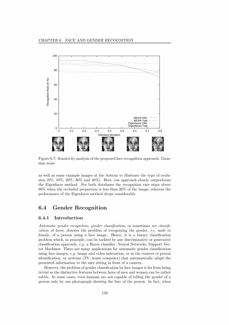
CHAPTER 6. FACE AND GENDER RECOGNITION
0
20
40
60
80
100
0 0.1 0.2 0.3 0.4 0.5 0.6 0.7 0.8
Rec
ogni
tion
Rat
e (in
%)
Standard deviation
MEAN ORLMEAN Yale
Eigenfaces ORLEigenfaces Yale
Figure 6.7: Sensitivity analysis of the proposed face recognition approach: Gaus-sian noise
as well as some example images at the bottom to illustrate the type of occlu-sion (0%, 10%, 20%, 30% and 40%). Here, our approach clearly outperformsthe Eigenfaces method. For both databases the recognition rate stays above80% when the occluded proportion is less than 20% of the image, whereas theperformance of the Eigenfaces method drops considerably.
6.4 Gender Recognition
6.4.1 Introduction
Automatic gender recognition, gender classification, or sometimes sex classifi-cation of faces, denotes the problem of recognizing the gender, i.e. male orfemale, of a person using a face image. Hence, it is a binary classificationproblem which, in principle, can be tackled by any discriminative or generativeclassification approach, e.g. a Bayes classifier, Neural Networks, Support Vec-tor Machines. There are many applications for automatic gender classificationusing face images, e.g. image and video indexation, or in the context of personidentification, or systems (TV, home computer) that automatically adapt thepresented information to the user sitting in front of a camera.
However, the problem of gender classification by face images is far from beingtrivial as the distinctive features between faces of men and women can be rathersubtle. In some cases, even humans are not capable of telling the gender of aperson only by one photograph showing the face of the person. In fact, when
133
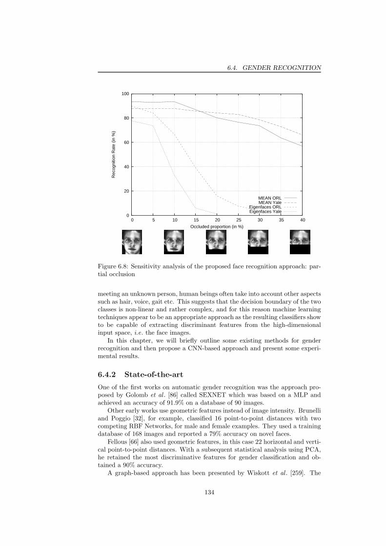
6.4. GENDER RECOGNITION
0
20
40
60
80
100
0 5 10 15 20 25 30 35 40
Rec
ogni
tion
Rat
e (in
%)
Occluded proportion (in %)
MEAN ORLMEAN Yale
Eigenfaces ORLEigenfaces Yale
Figure 6.8: Sensitivity analysis of the proposed face recognition approach: par-tial occlusion
meeting an unknown person, human beings often take into account other aspectssuch as hair, voice, gait etc. This suggests that the decision boundary of the twoclasses is non-linear and rather complex, and for this reason machine learningtechniques appear to be an appropriate approach as the resulting classifiers showto be capable of extracting discriminant features from the high-dimensionalinput space, i.e. the face images.
In this chapter, we will briefly outline some existing methods for genderrecognition and then propose a CNN-based approach and present some experi-mental results.
6.4.2 State-of-the-art
One of the first works on automatic gender recognition was the approach pro-posed by Golomb et al . [86] called SEXNET which was based on a MLP andachieved an accuracy of 91.9% on a database of 90 images.
Other early works use geometric features instead of image intensity. Brunelliand Poggio [32], for example, classified 16 point-to-point distances with twocompeting RBF Networks, for male and female examples. They used a trainingdatabase of 168 images and reported a 79% accuracy on novel faces.
Fellous [66] also used geometric features, in this case 22 horizontal and verti-cal point-to-point distances. With a subsequent statistical analysis using PCA,he retained the most discriminative features for gender classification and ob-tained a 90% accuracy.
A graph-based approach has been presented by Wiskott et al . [259]. The
134

CHAPTER 6. FACE AND GENDER RECOGNITION
nodes of the graph represent wavelet-based local appearances and the edges arelabeled with distance vectors. Using a small number of model graphs for maleand female face images they were able to classify new images by a special graphmatching procedure with a 91.2% classification accuracy.
O’Toole et al . [177] used a PCA-compressed representation of the imageintensities and classified them with a linear Perceptron.
PCA has also been used by Graf et al . [89] who compared it to Local LinearEmbedding (LLE), a non-linear neighborhood-preserving dimensionality reduc-tion technique. The authors then employ SVMs for the final gender classifica-tion. Sun et al . [230] additionally selected a subset of PCA features by a GeneticAlgorithm-based method and then compare different classification approaches,i.e. Bayes classifier, a LDA-based classifier, a Neural Network and a SVM, onthe gender recognition problem. BenAbdelKader and Griffin [18] also appliedPCA on the pixel intensities. For classification they compare a SVM approachwith Fisher’s Linear Discriminant.
A method using ICA for feature extraction has been proposed by Jain andHuang [113]. The final classification was performed by means of a LDA.
Buchala et al . [34] used a non-linear dimensionality reduction method calledCurvilinear Component Analysis (CCA) and then compared SVMs with MLPsfor gender classification.
Moghaddam and Yang [164] proposed an approach training an SVM classifierdirectly on the image pixel intensities. A correct gender classification rate of96.6% on the FERET database has been reported by the authors.
A different method is due to Gutta et al . [92]. Here, a mixture of expertscombines several classifiers, RBF ensembles, Inductive Decision Trees (IDT) andSVMs which were employed on different image regions. The authors reported aclassification rate of 96% on the FERET database.
Lanitis et al . [130] presented an approach that transforms the face imagesinto a shape-free patches using AAMs. The resulting images were then classi-fied using a Mahalanobis-based distance measure. AAMs have also been usedby Saatci et al . [209] for feature extraction. Here, gender recognition was per-formed by matching a trained AAM to the unknown face and finally classifyingthe resulting model parameters by a SVM. A classification of 97.6% has beenobtained on a set of several databases but the results only contain the caseswhere the AAM converged correctly.
Shakhnarovich et al . [222] presented an approach based on Adaboost. Theyproposed to use the features from the Boosted Cascade Detector for face de-tection from Viola and Jones [250] to perform gender classification and reportan accuracy of 79%. Recently, Baluja et al . [11] also proposed an Adaboost-based method. Here, they used features comparing pixel intensities for theirweak classifiers in the Adaboost procedure and compared it to a SVM-basedapproach. A maximum accuracy of over 93% has been achieved by their genderrecognition method on the FERET database.
Finally, the approach presented by Tivive and Bouzerdoum [241] uses Shunt-ing Inhibitory Convolutional Neural Networks (SICoNNets) (c.f . section 3.4.4).They obtained an 97.1% accuracy on the FERET database.
135

6.5. CONCLUSION
Figure 6.9: Examples of training images for gender classification. Left: men,right: women
6.4.3 Gender Recognition with Convolutional Neural Net-
works
We propose a gender recognition method [82] based on a Convolutional Neu-ral Network (CNN) architecture similar to the one of the Convolutional FaceFinder (CFF) from Garcia and Delakis [81] described in section 4.2.3. The onlysignificant change compared to the CFF architecture is the size of the featuremaps. The dimension of the retina of the gender recognition CNN is 46 × 56pixels. The size of feature maps of all of the other layers follows systematicallyfrom the retina dimension and the respective kernel sizes, i.e. 5× 5 kernels forthe first and a 3× 3 kernels for the second convolution layer. The sub-samplingwindow size is 2 × 2 as with the CFF. In the final layer there is a single neu-ron representing the classification result, i.e. the value −1 for male and +1 forfemale face images.
The training set was constructed using cropped and histogram-equalizedfrontal face images of the FERET database [183] (see Appendix A), where 80%of the images were used for training and 20% for testing. Figure 6.9 showssome training examples situated close to the border of the decision boundary.Training was then performed using the online Backpropagation algorithm forCNNs (see Alg. 8 on page 57).
The classification rate obtained with this architecture is 94.7% which is com-parable to the results obtained by [11] who reported a (maximal) classificationrate of 93.5% using a SVM-based and 94.4% using a Adaboost-based approach.Figure 6.10 shows the respective ROC curve of the test set.
Note that many existing gender classification methods mix the same per-sons across the training and test set when there are several examples of oneperson’s face, which obviously makes the problem easier as the algorithm might“memorize” specific individuals. In the preceding experiment, we put all ex-ample images of one particular person in either the training or the test test,demonstrating more soundly the generalization capacity of the system.
We also conducted an experiment with a mixed training set, i.e. the testimages were randomly selected from the whole database (FERET) such thatexample images of one person might be in the training and the test set. Asexpected, the recognition rate is higher than with the unmixed datasets: 97.4%of correct classification have been obtained with this setting, which is also com-parable to the results obtained by [11] where the best SVM achieves an accuracyof 97.1% and the best Adaboost classifier: 96.6%.
6.5 Conclusion
In this chapter, we presented a face recognition approach based on a specifictype of CNN which is trained to reconstruct reference images pre-defined for
136
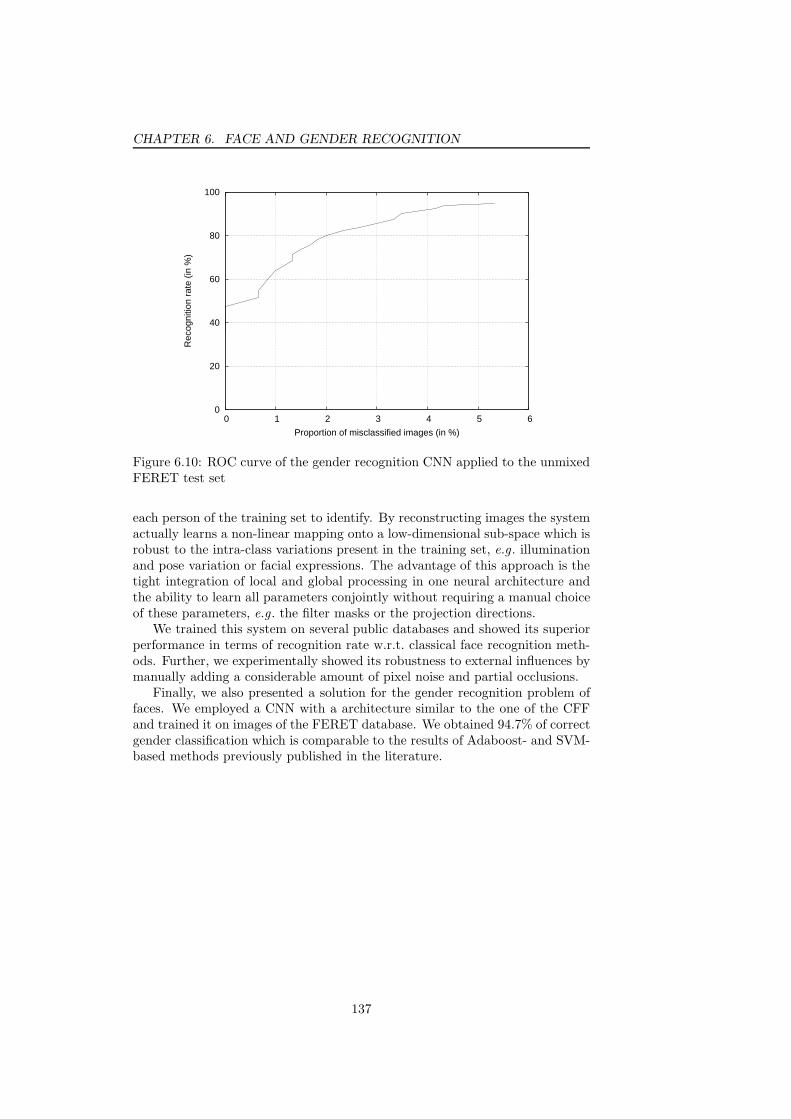
CHAPTER 6. FACE AND GENDER RECOGNITION
0
20
40
60
80
100
0 1 2 3 4 5 6
Rec
ogni
tion
rate
(in
%)
Proportion of misclassified images (in %)
Figure 6.10: ROC curve of the gender recognition CNN applied to the unmixedFERET test set
each person of the training set to identify. By reconstructing images the systemactually learns a non-linear mapping onto a low-dimensional sub-space which isrobust to the intra-class variations present in the training set, e.g. illuminationand pose variation or facial expressions. The advantage of this approach is thetight integration of local and global processing in one neural architecture andthe ability to learn all parameters conjointly without requiring a manual choiceof these parameters, e.g. the filter masks or the projection directions.
We trained this system on several public databases and showed its superiorperformance in terms of recognition rate w.r.t. classical face recognition meth-ods. Further, we experimentally showed its robustness to external influences bymanually adding a considerable amount of pixel noise and partial occlusions.
Finally, we also presented a solution for the gender recognition problem offaces. We employed a CNN with a architecture similar to the one of the CFFand trained it on images of the FERET database. We obtained 94.7% of correctgender classification which is comparable to the results of Adaboost- and SVM-based methods previously published in the literature.
137

Chapter 7
Conclusion and
Perspectives
7.1 Conclusion
In this work, we described the problem of automatic appearance-based facialanalysis and outlined some of the most common techniques to tackle it. We par-ticularly focused on an approach called Convolutional Neural Network (CNN)which is a connectionist model inspired by biological findings in the visual sys-tem of mammals. Being initially used for handwritten digit recognition it hasmeanwhile been successfully applied to many other visual pattern recognitionproblems. For example, the CNN-based face detection system proposed by Gar-cia and Delakis [81] shows to be very robust against most types of noise andexternal influences that face images can undergo in real-world settings, andthe results are superior to other state-of-the-art appearance-based classificationmethods evaluated on common public databases.
Using CNN models that are, in a way, similar to the ones mentioned above,we proposed effective approaches to different facial analysis problems. The firstsystem we presented tackles the problem of face alignment which is a crucialstep in many facial image processing applications, notably face recognition. Thisprocedure is typically performed after face detection and before face recogni-tion, and its purpose is to align the bounding rectangles coming from the facedetection system such that specific facial features are roughly at predefined po-sitions inside the images bounded by the respective rectangles. The proposedapproach is based on a specific CNN architecture that learns the parameters ofthis type of affine transformation, i.e. x/y translation, rotation angle and scalefactor, by means of annotated mis-aligned face images. The trained systemis then able to conjointly estimate these four transformation parameters whenpresenting a mis-aligned face image at its input without explicitely localizingspecific facial features such as the eyes. We experimentally showed that in aniterative approach, it is able to precisely and robustly correct the boundingrectangles coming from a face detector such that they are well-aligned with thefaces inside the respective rectangles. A correct alignment rate of 94% for ourown test set containing difficult images and 80% for the public BioID databasehas been obtained while tolerating a mean distance from the desired bounding
138

CHAPTER 7. CONCLUSION AND PERSPECTIVES
rectangle corners of 10% of the rectangle’s width.
Then, we presented a central problem in facial analysis, called facial featuredetection, i.e. the localization of characteristic feature points in face images. Wefurther proposed a CNN-based approach to this problem which, in a hierarchicalmanner, localizes 10 facial feature points in face images taken under difficultconditions. The system correctly localizes the 10 points of 96% of the faces ofthe AR database and 87% of the BioID database tolerating an error of 10% ofthe inter-ocular distance. We also measured the precision of eye pupil detectionfor the BioID database and showed that our approach outperforms state-of-the-art systems. Different types of input features to the CNN have been tried,while normalized image intensities gave the best results compared to gradientsand Gabor wavelet filter responses. Finally, we demonstrated the considerablyhigh robustness of the proposed approach w.r.t. Gaussian pixel noise and partialocclusions.
In the subsequent chapter, we described the problems of automatic facerecognition and gender classification. For the former task, we proposed a novelapproach based on a specific CNN architecture which learns a non-linear map-ping from the image space onto a lower-dimensional sub-space. By learningto reconstruct reference images for each person to classify the system buildsa sub-space less sensitive to the intra-class variations present in the trainingset. The recognition rate obtained in our experiments on the public databasesORL and Yale is 93%, which is higher than the one obtained with the classicalface recognition methods: Eigenfaces and Fisherfaces. As with the other pro-posed approaches, we also showed the robustness of the system w.r.t. Gaussianpixel noise and partial occlusions. Finally, we presented a gender classificationmethod based on a model similar to the CNN used in the face detection systemof Garcia and Delakis [81]. The system is able to correctly recognize the genderof 94.7% of the face images of a test set extracted from the FERET databasewhen images of the same individuals are not mixed across the training and testset. This result is comparable to recognition rates of state-of-the-art systemsbased on SVMs or Adaboost.
To sum up, one can say that the CNN approach is a very powerful machinelearning technique capable of learning very complex non-linear functions relatedto appearance-based pattern recognition. The advantage of CNNs is that theyautomatically learn adapted filters that extract non-linear characteristic featuresuseful for a dedicated classification task. This integrated learning procedureof all inherent parameters using the Backpropagation paradigm and a globalerror function to minimize circumvents the somewhat tedious task of “manual”parameter determination of feature extractors and classifiers. Additionally, thepossibility to easily implement CNNs on embedded and parallel platforms andto build dedicated real-time systems is a big advantage of this approach.
However, the drawback of this technique is the “manual” determination ofthe topology of the CNNs for a given task as well as the creation of a sufficientlylarge and appropriate training database. This leads us to the final section ofthis work which addresses some perspectives of future research in this field.
139

7.2. PERSPECTIVES
7.2 Perspectives
7.2.1 Convolutional Neural Networks
As mentioned in the previous section, the architecture of a CNN best suitedfor a given task is determined empirically, which is undoubtedly a sub-optimalchoice. It would however be preferable to automatically adapt the complexityof the model to the complexity of the problem in order to reduce the size ofthe CNN and increase its generalization capacity. Many works have been con-ducted in this area, e.g. with respect to constructive neural networks, growingand pruning techniques or incremental learning. However most of them areconcerned with standard neural architectures, e.g. MLPs, and do not cope withmore complicated models such as CNNs which have specific types of architec-tures employing weight sharing.
Another interesting issue would be to investigate the ability of a CNN tolearn from a reduced set of training examples while obtaining equal or almostequal results than with a larger training set. This implies either a technique toautomatically select from a large set the most significant training examples fora given task or – if a larger training set is not available – a method to constructa type of model on the reduced training set and to integrate this model into thetraining procedure.
Finally, CNNs which are able to extract features invariant to larger trans-lations, rotations and changes in scale would be an interesting area of futureresearch. The works by Ranzato et al . [193] on shift-invariant feature extractionusing a CNN-based encoder-decoder framework (c.f . section 3.4.5) are particu-larly promising in this regard. In this context, another interesting perspectivecould be pursued: the application of CNNs to whole scenery images in order toextract prominent feature points helping to classify these images or particularvisual objects. This type of CNN could then be considered as a specialized andlearned interest point detector and/or descriptor.
7.2.2 Facial analysis with Convolutional Neural Networks
Many face analysis problems, like face recognition under unconstrained real-world conditions, are still far from being resolved. Variations in illumination,head pose and facial expressions represent the biggest difficulties for most of thecurrent solutions including CNNs. In this work, we haven’t explicitely modeledthese variations but learned them implicitly using training images taken underdifferent conditions. An interesting direction of future research would thus beto integrate this type of model into the proposed CNN-based systems and in-vestigate the its impact on the overall performance. An initial approach couldbe to train a CNN to estimate or even to correct the illumination of a faceusing annotated training examples. One could also imagine a CNN-based headpose estimator, the results of which could then be used for further view-specificprocessing, e.g. face recognition.
Finally, CNNs are not limited to gray scales but can also process color im-ages, i.e. by simply presenting three images corresponding to the different colorchannels (e.g. red, green and blue) at the input. However, as experimental re-sults on face detection show, the use of color might have a negative impact onthe robustness of the system especially with respect to different lighting condi-
140

CHAPTER 7. CONCLUSION AND PERSPECTIVES
tions. Nevertheless, the ability of CNNs to process multi-dimensional data is avery interesting perspective as they could for example be applied to many typesof multi-modal data, e.g. images and sound, images of different views, or videoframes at different time steps etc. One could also imagine to process 3D databy CNNs, or to fuse 2D and 3D data, e.g. for face recognition.
Many interesting research directions in the domain of automatic facial anal-ysis are to be explored. Convolutional Neural Networks represent a promisingapproach from the computational side but perhaps also novel biological and/orneuro-scientific results will yield further ideas to improve this model.
141

Appendix A
Excerpts from the used face
databases
A.1 AR
142
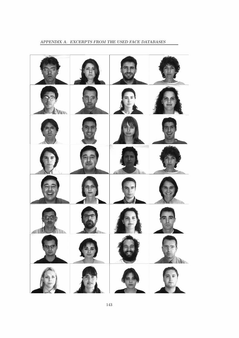
APPENDIX A. EXCERPTS FROM THE USED FACE DATABASES
143

A.2. BIOID
A.2 BioID
144

APPENDIX A. EXCERPTS FROM THE USED FACE DATABASES
145

A.3. FERET
A.3 FERET
146

APPENDIX A. EXCERPTS FROM THE USED FACE DATABASES
147

A.4. GOOGLE IMAGES
A.4 Google Images
148
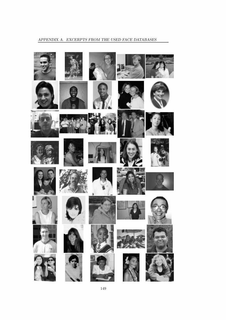
APPENDIX A. EXCERPTS FROM THE USED FACE DATABASES
149

A.5. ORL
A.5 ORL
150

APPENDIX A. EXCERPTS FROM THE USED FACE DATABASES
151

A.6. PIE
A.6 PIE
152

APPENDIX A. EXCERPTS FROM THE USED FACE DATABASES
153
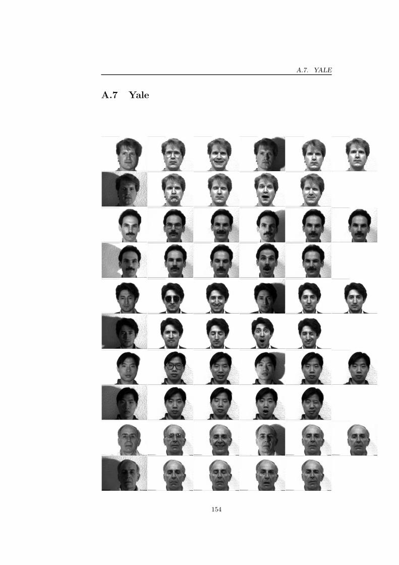
A.7. YALE
A.7 Yale
154
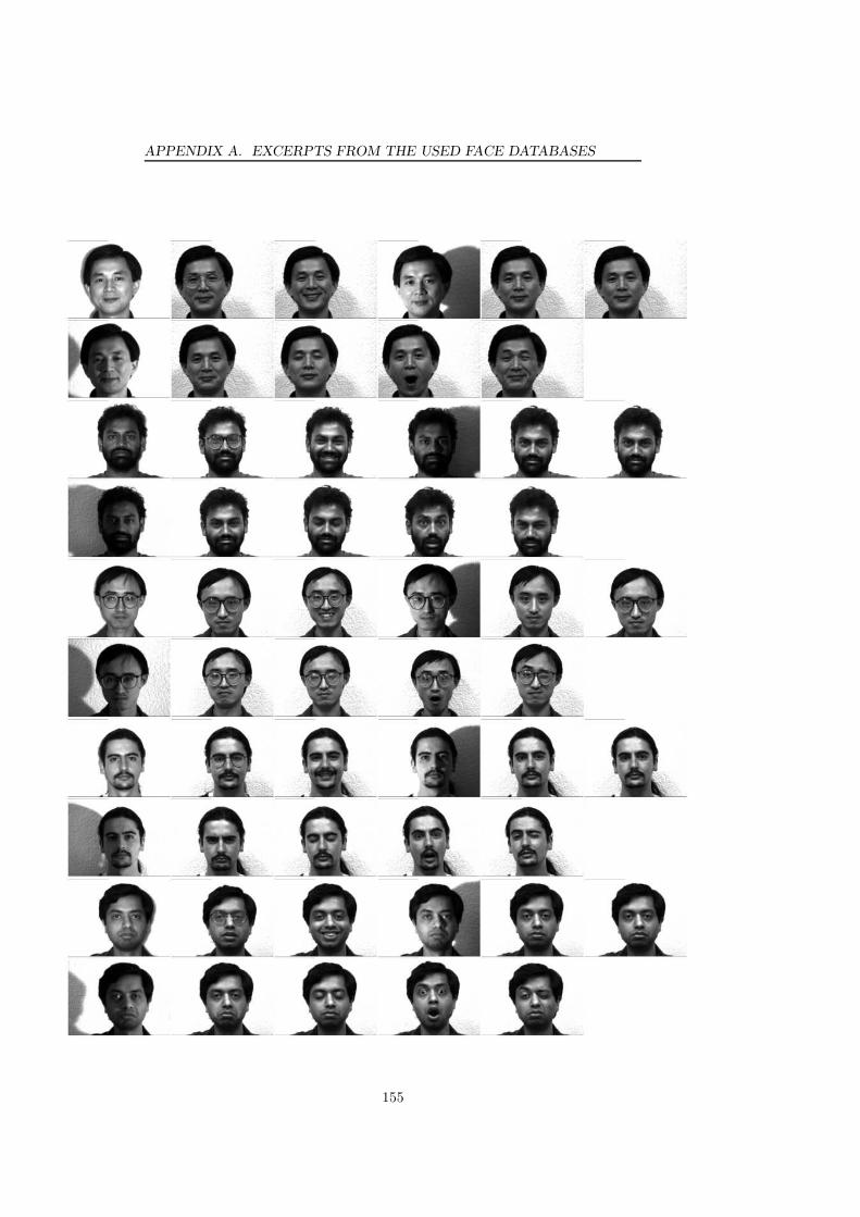
APPENDIX A. EXCERPTS FROM THE USED FACE DATABASES
155

Bibliography
[1] L. B. Almeida, T. Langlois, J. D. Amaral, and A. Plakhov. Parameteradaptation in stochastic optimization. In D. Saad, editor, On-Line Learn-ing in Neural Networks, chapter 6. Cambridge University Press, 1999.
[2] S.-I. Amari, A. Cichocki, and H. Yang. A new learning algorithm for blindsource separation. In D. S. Touretzky, M. C. Moser, and M. E. Hasselmo,editors, Advances in Neural Information Processing Systems, volume 8,pages 757–763. MIT Press, Cambridge, MA, 1996.
[3] G. Arulampalam and A. Bouzerdoum. A generalized feedforward neuralnetwork architecture for classification and regression. Neural Networks,16:561–568, 2003.
[4] A. Azarbayejani, T. Starner, B. Horowitz, and A. Pentland. Visuallycontrolled graphics. IEEE Transactions on Pattern Analysis and MachineIntelligence, 15(6):602–605, June 1993.
[5] S. O. Ba and J. M. Odobez. A probabilistic framework for joint head track-ing and pose estimation. In Proceedings of the 17th International Confer-ence on Pattern Recognition, volume 4, pages 264–267, August 2004.
[6] F. R. Bach and M. I. Jordan. Kernel independent component analysis.Journal of Machine Learning Research, 3:1–48, 2002.
[7] E. Bailly-Bailliere, S. Bengio, F. Bimbot, M. Hamouz, J. Kittler, J. Marie-thoz, J. Matas, K. Messer, V. Popovici, F. Poree, B. Ruiz, and J.-P. Thi-ran. The BANCA database and evaluation protocol. In Proceedings of theFourth International Conference on Audio- and Video-Based BiometricPerson Authentication, pages 625–638, 2003.
[8] S. Baker and I. Matthews. Equivalence and efficiency of image alignmentalgorithms. In Computer Vision and Pattern Recognition, volume 1, pages1090–1097, 2001.
[9] P. Baldi and K. Hornik. Neural networks and principal component anal-ysis: Learning from examples without local minima. IEEE Transactionson Neural Networks, 2:53–58, 1988.
[10] S. Baluja. Probabilistic modeling for face orientation discrimination:Learning from labeled and unlabeled data. In Neural Information Pro-cessing Systems, 1998.
156

BIBLIOGRAPHY
[11] S. Baluja and H. A. Rowley. Boosting sex identification performance.International Journal of Computer Vision, 71(1):111–119, 2007.
[12] M. S. Bartlett, J. R. Movellan, and T. J. Sejnowski. Face recognition byindependent component analysis. IEEE Transactions on Neural Networks,13(6):1450–1464, 2002.
[13] R. Basri and D. Jacobs. Lambertian reflectance and linear subspaces. InInternational Conference on Computer Vision, volume 2, pages 383–390,2001.
[14] R. Battiti. Accelerated backpropagation learning: Two optimizationmethods. Complex Systems, 3:331–342, 1989.
[15] P. Belhumeur, J. Hespanha, and D. Kriegman. What is the set of imagesof an object under all possible lighting conditions. International Journalof Computer Vision, 28(3):245–260, 1998.
[16] P. N. Belhumeur, J. P. Hespanha, and D. J. Kriegmann. Eigenfacesvs Fisherfaces: Recognition using class specific linear projection. IEEETransactions on Pattern Analysis and Machine Intelligence, 17(7):711–720, 1997.
[17] A. Bell and T. Sejnowski. An information maximization approach to blindseparation and blind deconvolution. Neural Computation, 7:1129–1159,1995.
[18] C. BenAbdelKader and P. Griffin. A local region-based approach to genderclassification from face images. In Proceedings of the IEEE Conference onComputer Vision and Pattern Recognition, 2005.
[19] Y. Bengio, Y. LeCun, and D. Henderson. Globally trained handwrittenword recognizer using spatial representation, space displacement neuralnetworks and hidden markov models. In Advances in Neural InformationProcessing Systems, volume 6, pages 937–944. Morgan Kaufmann, 1994.
[20] T. L. Berg, A. C. Berg, J. Edwards, M. Maire, R. White, Yee-Whye Teh,E. Learned-Miller, and D. A. Forsyth. Names and faces in the news.In Proceedings of the International Conference on Computer Vision andPattern Recognition, volume 2, pages 848–854, 2004.
[21] D. Beymer and T. Poggio. Face recognition from one example view. AIMemo 1536, MIT AI Lab, 1995.
[22] The BioID face database. http://www.humanscan.com/support/downloads/facedb.php.
[23] B. E. Boser, I. M. Guyon, and V. Vapnik. A training algorithm for optimalmargin classifiers. In Fifth Annual Workshop on Computational LearningTheory, pages 144–152, Pittsburgh ACM, 1992.
[24] H. Bourlard and Y. Kamp. Auto-association by multilayer perceptronsand singular value decomposition. Biological Cybernetics, 59:291–294,1988.
157

BIBLIOGRAPHY
[25] A. Bouzerdoum. The elementary movement detection mechanism in insectvision. In Philosophical Transactions: Biological Sciences, volume B-339,pages 375–384, 1993.
[26] A. Bouzerdoum. Classifiation and function approximation using feed-forward shunting inhibitory artificial neural networks. In Proceedings ofthe International Joint Conference on Neural Networks, pages 613–618,2000.
[27] A. Bouzerdoum and R. B. Pinter. Nonlinear lateral inhibition applied tomotion detection in the fly visual system. In R. B. Pinter and B. Nabet,editors, Nonlinear Vision, pages 423–450. Boca Raton, 1992.
[28] A. Bouzerdoum and R. B. Pinter. Shunting inhibitory cellular neuralnetworks: Derivation and stability analysis. IEEE Transactions on Cir-cuits and Systems I: Fundamental Theory and Applications, 40(3):215–221, March 1993.
[29] J. Bromley, I. Guyon, Y. LeCun, E. Sackinger, and R. Shah. Signatureverification using a ”siamese” time delay neural network. InternationalJournal of Pattern Recognition and Artificial Intelligence, 7(4):669–688,1993.
[30] D. Broomhead and D. Lowe. Multivariable functional interpolation andadaptive networks. Complex Systems, 2:312–355, 1988.
[31] L. M. Brown and Y. L. Tian. Comparative study of coarse head pose esti-mation. IEEE Workshop on Motion and Video Computing, 6, December2002.
[32] R. Brunelli and T. Poggio. HyperBF networks for gender classification.In DARPA Image Understanding Workshop, pages 311–314, 1992.
[33] Roberto Brunelli and Tomaso Poggio. Face recognition: Features versustemplates. IEEE Transactions on Pattern Analysis and Machine Intelli-gence, 15(10):1042–1052, 1993.
[34] S. Buchala, N. Davey, R. J. Frank, and T. M. Gale. Dimensionality reduc-tion of face images for gender classification. In Proceedings of the IEEEConference on Intelligent Systems, 2004.
[35] J. F. Cardoso. Higher-order contrasts for independent component analysis.Neural Computation, 11(1):157–192, 1999.
[36] H. Cevikalp, M. Neamtu, M. Wilkes, and A. Barkana. Discriminative com-mon vectors for face recognition. IEEE Transactions on Pattern Analysisand Machine Intelligence, 27(1):4–13, 2005.
[37] L. W. Chan and F. Fallside. An adaptive learning algorithm for back-propagation networks. Computer Speech and Language, 2:205–218, 1987.
[38] Qian Chen, Haiyuan Wu, T. Fukumoto, and M. Yachida. 3D head poseestimation without feature tracking. In Proceedings of the Third IEEE In-ternational Conference on Automatic Face and Gesture Recognition, pages88–93, April 1998.
158

BIBLIOGRAPHY
[39] Sumit Chopra, Raia Hadsell, and Yann LeCun. Learning a similarity met-ric discriminatively, with application to face verification. In Proceedingsof the International Conference on Computer Vision and Pattern Recog-nition. IEEE Press, 2005.
[40] A. J. Colmenarez and T. S. Huang. Face detection with information-based maximum discrimination. In Proceedings of the IEEE Conferenceon Computer Vision and Pattern Recognition, pages 782–787, 1997.
[41] T. Cootes, G. Edwards, and C. Taylor. Active appearance models. IEEETransactions on Pattern Analysis and Machine Intelligence, 23(6):681–685, 2001.
[42] T. F. Cootes and C. J. Tayler. Locating faces using statistical featuredetectors. In International Conference on Automatic Face and GesturesRecognition, pages 204–211, Los Alamitos, California, October 1996. IEEEComputer Society Press.
[43] T. F. Cootes, C. J. Taylor, D. H. Cooper, and J. Graham. Active shapemodels–their training and application. Computer Vision Graphics andImage Understanding, 61(1):38–59, 1995.
[44] C. Cortes and V. Vapnik. Support vector networks. Machine Learning,20:1–25, 1995.
[45] G. Cottrell and M. Fleming. Face recognition using unsupervised fea-ture extraction. In Proceedings of the International Conference on NeuralNetworks, pages 322–325, 1990.
[46] G. Cottrell and J. Metcalfe. EMPATH: Face, emotion, and gender recogni-tion using holons. In R. Lippmann, J. Moody, and D. Touretzky, editors,Advances in Neural Information Processing Systems 3, pages 564–571.Morgan Kaufmann, 1991.
[47] G. Cottrell, P. Munro, and D. Zipser. Learning internal representationsfrom gray-scale images: an example of extensional programming. In Pro-ceedings of the 9th Annual Conference of the Cognitive Science Society,pages 462–473, Seattle, WA, 1987.
[48] T. M. Cover. Geometrical and statistical properties of systems of linearinequalities with applications in pattern recognition. IEEE Transactionson Electronic Computers, 14:326–334, 1965.
[49] D. Cristinacce and T. Cootes. A comparison of shape constrained facialfeature detectors. In Proceedings of the 6th International Conference onAutomatic Face and Gesture Recognition, pages 375–380, Seoul, Korea,2004.
[50] D. Cristinacce, T. Cootes, and I. Scott. A multi-stage approach to facialfeature detection. In Proceedings of the British Machine Vision Confer-ence, pages 277–286, 2004.
[51] G. Csurka, C. Bray, C. Dance, and L. Fan. Visual categorization with bagsof keypoints. In ECCV Workshop on Statistical Learning in ComputerVision, pages 327–334, 2004.
159

BIBLIOGRAPHY
[52] Hasan Demirel, Thomas J. Clarke, and Peter Y. K. Cheung. Adaptiveautomatic facial feature segmentation. In Proceedings of the Second In-ternational Conference on Automatic Face and Gesture Recognition, pages277–282, 1996.
[53] S. Duffner and C. Garcia. A connexionist approach for robust and pre-cise facial feature detection in complex scenes. In Fourth InternationalSymposium on Image and Signal Processing and Analysis (ISPA), pages316–321, Zagreb, Croatia, September 2005.
[54] S. Duffner and C. Garcia. A hierarchical approach for precise facial featuredetection. In Compression et Representation des Signaux Audiovisuels(CORESA), pages 29–34, Rennes, France, November 2005.
[55] S. Duffner and C. Garcia. A neural scheme for robust detection of trans-parent logos in TV programs. In International Conference on Artifi-cial Neural Networks (ICANN), volume 2, pages 14–23, Athens, Greece,September 2006.
[56] S. Duffner and C. Garcia. Face recognition using non-linear image re-construction. In International Conference on Advanced Video and Signal-Based Surveillance (AVSS), London, UK, September 2007.
[57] S. Duffner and C. Garcia. An online backpropagation algorithm withvalidation error-based adaptive learning rate. In International Conferenceon Artificial Neural Networks (ICANN), volume 1, pages 249–258, Porto,Portugal, September 2007.
[58] S. Duffner and C. Garcia. Robust face alignment using convolutional neu-ral networks. In Proceedings of the International Conference on ComputerVision Theory and Applications (VISAPP), Funchal, Portugal, January2008. accepted.
[59] S. Duffner and C. Garcia. Robust hierarchical detection of facial featuresin complex scenes. Pattern Analysis & Applications, 2008. accepted.
[60] G. J. Edwards, C. J. Taylor, and T. F. Cootes. Interpreting face imagesusing active appearance models. In Proceedings of the IEEE Conferenceon Automatic Face and Gesture Recognition, pages 300–305, April 1998.
[61] E. Elagin, J. Steffens, and H. Neven. Automatic pose estimation system forhuman faces based on bunch graph matching technology. In Proceedings ofthe Third IEEE International Conference on Automatic Face and GestureRecognition, pages 136–141, April 1998.
[62] M. J. Er, S. Wu, J. Lu, and H. L. Toh. Face recognition with radial basisfunction (RBF) neural networks. IEEE Transactions on Neural Networks,13:697–709, 2002.
[63] S. E. Fahlman. Faster-learning variations on back-propagation: An empir-ical study. In D. S. Touretzky, G. E. Hinton, and T. J. Sejnowski, editors,Connectionist Models Summer School, pages 38–51. Morgan KaufmannPublishers, San Mateo, CA, 1988.
160

BIBLIOGRAPHY
[64] B. Fasel. Multiscale facial expression recognition using convolutional neu-ral networks. In Proceedings of the Third Indian Conference on ComputerVision, Graphics and Image Processing, Ahmedabad, India, 2002.
[65] B. Fasel. Robust face analysis using convolutional neural networks. InProceedings of the 16th International Conference on Pattern Recognition,volume 2, pages 40–43, Quebec, Canada, 2002.
[66] J.-M. Fellous. Gender discrimination and predication on the basis of facialmetric information. Vision Research, 37:1961–1973, 1997.
[67] R. Feraud, O. Bernier, J.-E. Viallet, and M. Collobert. A fast and accurateface detector based on neural networks. IEEE Transactions on PatternAnalysis and Machine Intelligence, 23(1):42–53, 2002.
[68] R. S. Feris, J. Gemmell, K. Toyama, and V. Kruger. Hierarchical waveletnetworks for facial feature localization. In Proceedings of the Fifth IEEEInternational Conference on Automatic Face and Gesture Recognition,2002.
[69] R. A. Fisher. The use of multiple measures in taxonomic problems. Annalsof Eugenics, 17:179–188, 1936.
[70] Yoav Freund and Robert E. Schapire. A decision-theoretic generalizationof on-line learning and an application to boosting. In Second InternationalConference on Computational Learning Theory, 1995.
[71] Yoav Freund and Robert E. Schapire. A decision-theoretic generalizationof on-line learning and an application to boosting. Journal of Computerand System Sciences, 55(1):119–139, August 1997.
[72] B. Froba and C. Kullbeck. Orientation template matching for face local-ization in complex visual scenes. In International Conference on ImageProcessing, pages 251–254, 2000.
[73] K. Fukushima. Cognitron: A self-organizing multilayered neural network.Biological Cybernetics, 20:121–136, 1975.
[74] K. Fukushima. Neocognitron: A self-organizing neural-network modelfor a mechanism of pattern recognition unaffected by shift in position.Biological Cybernetics, 36:193–202, 1980.
[75] K. Fukushima. A neural-network model for selective attention in visualpattern recognition. Biological Cybernetics, 55:5–15, 1986.
[76] K. Fukushima. Analysis of the process of visual pattern recognition bythe neocognitron. Neural Networks, 2:413–421, 1989.
[77] K. Fukushima and T. Imagawa. Recognition and segmentation of con-nected characters with selective attention. Neural Networks, 6:33–41,1993.
[78] K. Fukushima and N. Wake. Handwritten alphanumeric character recog-nition by the neocognitron. IEEE Transactions on Neural Networks,2(3):335–365, May 1991.
161

BIBLIOGRAPHY
[79] Ken-ichi Funahashi. On the approximate realization of identity mappingsby three-layer neural networks. Technical report, Toyohashi University ofTechnology, Department of Information and Computer Sciences, 1990.
[80] Y. Gao and K. H. Leung. Face recognition using line edge map. IEEETransactions on Pattern Analysis and Machine Intelligence, 24(6):764–779, 2002.
[81] C. Garcia and M. Delakis. Convolutional face finder: A neural architecturefor fast and robust face detection. IEEE Transactions on Pattern Analysisand Machine Intelligence, 26(11):1408–1423, 2004.
[82] C. Garcia and S. Duffner. Facial image processing with convolutional neu-ral networks. In International Workshop on Advances in Pattern Recog-nition (IWAPR), pages 97–108, Plymouth, United Kingdom, July 2007.
[83] C. Garcia, G. Simantiris, and G. Tziritas. A feature-based face detectorusing wavelet frames. In Intern. Workshop on Very Low Bitrate VideoCoding, pages 71–76, Athens, 2001.
[84] A. S. Georghiades, P. N. Belhumeur, and D. J. Kriegman. From fewto many: illumination cone models for face recognition under variablelighting and pose. IEEE Transactions on Pattern Analysis and MachineIntelligence, 23(6):643–660, June 2001.
[85] A. Gepperth. Visual object classification by sparse convolutional neuralnetworks. In Proceedings of the European Symposium on Artificial NeuralNetworks, 2006.
[86] B. A. Golomb, D. T. Lawrence, and T. J. Sejnowski. Sexnet: A neuralnetwork identifies sex from human faces. In R. Lippmann, J. Moody, andD. Touretzky, editors, Advances in Neural Information Processing Systems3, pages 572–577. Morgan Kaufmann, 1991.
[87] S. Gong, S. McKenna, and J. Collins. An investigation into face posedistributions. In Proceedings of the 2nd International Workshop on Auto-matic Face and Gesture Recognition, pages 265–270, 1996.
[88] Nicolas Gourier, Daniela Hall, and James L. Crowley. Facial feature de-tection robust to pose, illumination and identity. In Proceedings of theIEEE International Conference on Systems, Man and Cybernetics, 2004.
[89] A. B. A. Graf and F. A. Wichmann. Gender classification of human faces.Biologically Motivated Computer Vision, pages 491–501, 2002.
[90] R. Gross, J. Shi, and J. Cohn. Quo vadis face recognition? In ThirdWorkshop on Empirical Evaluation Methods in Computer Vision, Decem-ber 2001.
[91] S. Grossberg, editor. Neural Networks and Natural Intelligence. MITPress, Cambridge, MA, 1988.
[92] S. Gutta, J. R. J. Huang, P. Jonathon, and H. Wechsler. Mixture ofexperts for classification of gender, ethnic origin, and pose of human faces.IEEE Transactions on Neural Networks, 11(4):948–960, July 2000.
162
BIBLIOGRAPHY
[93] M. Hamouz, J. Kittler, J.-K. Kamarainen, P. Paalanen, and H. Kalvi-ainen. Affine-invariant face detection and localization using GMM-basedfeature detectors and enhanced appearance model. In Proceedings of theSixth International Conference on Automatic Face and Gesture Recogni-tion, pages 67–72, 2004.
[94] M. Hamouz, J. Kittler, J.-K. Kamarainen, P. Paalanen, H. Kalviainen,and J. Matas. Feature-based affine-invariant localization of faces. IEEETransactions on Pattern Analysis and Machine Intelligence, 27(9):1490–1495, 2005.
[95] M.E. Harmon and L.C. Baird III. Multi-player residual advantage learningwith general function approximation. Technical report, Wright Labora-tory, WL/AACF, Wright-Patterson Air Force Base, OH, 1996.
[96] B. Heisele, P. Ho, J. Wu, and T Poggio. Face recognition: component-based versus global approaches. Computer Vision and Image Understand-ing, 91(1):6–21, 2003.
[97] B. Heisele, T. Poggio, and M. Pontil. Face detection in still gray images.AI Memo 1687, Center for Biological and Computational Learning, MIT,Cambridge, MA, 2000.
[98] E. Hjelmas and B. K. Low. Face detection: A survey. Computer Visionand Image Understanding, 83:236–274, 2001.
[99] B. K. P Horn. Shape from Shading: A Method for Obtaining the Shapeof a Smooth Opaque Object from One View. PhD thesis, MassachusettsInstitute of Technology, 1970.
[100] B. K. P. Horn and M. J. Brooks. Shape from Shading. MIT Press: Cam-bridge, MA, 1989.
[101] H. J. Hotelling. Analysis of statistical variables into principal components.Journal of Educational Psychology, 24:417–441, 1933.
[102] H.-C. Hsin, C.-C. Li, M. Sun, and R.J. Sclabassi. An adaptive trainingalgorithm for back-propagation neural networks. In International Con-ference on Systems, Man and Cybernetics, volume 2, pages 1049–1052,1992.
[103] C. Hu, R. Feris, and M. Turk. Active wavelet networks for face alignment.In British Machine Vision Conference, UK, 2003.
[104] C. Huang, B. Wu, H. Ai, and S. Lao. Omni-directional face detectionbased on real adaboost. In Proceedings of the International Conferenceon Image Processing, Singapore, 2004.
[105] J. Huang, X. Shao, and H. Wechsler. Face pose discrimination usingsupport vector machines (SVM). In Proceedings of the Fourteenth Inter-national Conference on Pattern Recognition, volume 1, pages 154–156,August 1998.
163
BIBLIOGRAPHY
[106] D. Hubel and T. Wiesel. Receptive fields, binocular interaction andfunctional architecture in the cat’s visual cortex. Journal of Physiology,160:106–154, 1962.
[107] A. Hyvarinen. Fast and robust fixed-point algorithms for independentcomponent analysis. IEEE Transactions on Neural Networks, 10:626–634,1999.
[108] A. Hyvarinen, J. Karhunen, and E. Oja. Independent Component Analysis.Wiley, New York, 2001.
[109] A. Hyvarinen and E. Oja. A fast fixed-point algorithm for independentcomponent analysis. Neural Computation, 9(7):1483–1492, 1997.
[110] K. Ikeuchi and B. K. P. Horn. Numerical shape from shading and occlud-ing boundaries. Artificial Intelligence, 17:141–184, 1981.
[111] N. Intrator, D. Reisfeld, and Y. Yeshurun. Extraction of facial featuresfor recognition using neural networks. In Proceedings of the InternationalWorkshop on Automatic Face and Gesture Recognition, pages 260–265,Zurich, 1995.
[112] R. A. Jacobs. Increased rates of convergence through learning rate adap-tion. Neural Networks, 1:295–307, 1988.
[113] A. Jain and J. Huang. Integrating independent components and lineardiscriminant analysis for gender classification. In Proceedings of the Inter-national Conference on Automatic Face and Gesture Recognition, 2004.
[114] N. Japkowitz, S. Hanson, and A. Gluck. Nonlinear autoassociation is notequivalent to PCA. Neural Computation, 12(3):531–545, 2000.
[115] S. Jeng, H. Yao, C. Han, M. Chern, and Y. Liu. Facial feature detectionusing geometrical face model: An efficient approach. Pattern Recognition,31(3):273–282, 1998.
[116] O. Jesorsky, K. J. Kirchberg, and R. W. Frischholz. Robust face detectionusing the hausdorff distance. In J. Bigun and F. Smeraldi, editors, ThirdInternational Conference on Audio- and Video-Based Biometric PersonAuthentication (AVBPA), volume 2091 of Lecture Notes in Computer Sci-ence, pages 90–95, Halmstad, Sweden, 2001. Springer.
[117] K. Jia, S. Gong, and A. P. Leung. Coupling face registration and super-resolution. In British Machine Vision Conference, pages 449–458, Edin-burg, UK, September 2006.
[118] M. Jones and P. Viola. Fast multi-view face detection. Technical ReportTR2003-96, Mitsubishi Electric Research Laboratories, 2003.
[119] K. Jonsson, J. Kittler, Y. Li, and J. Matas. Learning support vectors forface verification and recognition. In Proceedings of the IEEE Conferenceon Automatic Face and Gesture Recognition, pages 208–213, 2000.
[120] C. Jutten and J. Herault. Blind separation of sources. Signal Processing,24:1–10, 1991.
164

BIBLIOGRAPHY
[121] J. Keeler, D. Rumelhart, and W. Leow. Integrated segmentation andrecognition of hand-printed numerals. Neural Information processing Sys-tems, 3:557–563, 1991.
[122] M. Kirby and L. Sirovich. Application of the Karhunen-Loeve procedurefor the characterization of human faces. IEEE Transactions on PatternAnalysis and Machine Intelligence, 12(1):103–108, 1990.
[123] T. Kohonen. Self-organizing formation of topologically correct featuremaps. Biological Cybernetics, 43(1):59–69, 1982.
[124] T. Kohonen. Self-Organizing and Associative Memory. Springer-Verlag,Berlin, 1989.
[125] M. A. Kramer. Nonlinear principal component analysis using autoasso-ciative neural networks. AIChE Journal, 37:233–243, 1991.
[126] B. Kruger, S. Bruns, and G. Sommer. Efficient head pose estimation withgabor wavelet networks. In Proceedings of the 11th British Machine VisionConference, volume 1, pages 72–81, September 2000.
[127] N. Kruger, M. Potzsch, and C. von der Malsburg. Estimation of faceposition and pose with labeled graphs. Proceedings of the British MachineVision Conference, pages 735–743, 1996.
[128] N. Kumar, V. Abhishek, and G. Gautam. A novel approach for personauthentication and content-based tracking in videos using kernel methodsand active appearance models. In Proceedings of the IEEE Conference onSystems, Man and Cybernetics, volume 2, pages 1384–1389, 2003.
[129] M. Lando and S. Edelman. Generalization from a single view in facerecognition. In International Workshop on Automatic Face- and GestureRecognition, 1995.
[130] A. Lanitis, C. J. Taylor, and T. Cootes. Automatic interpretation andcoding of face images using flexible models. IEEE Transactions on PatternAnalysis and Machine Intelligence, 19(7):743–756, July 1997.
[131] A. Lanitis, C. J. Taylor, and T. F. Cootes. Automatic face identificationsystem using flexible appearance models. Image and Vision Computing,13:393–401, 1995.
[132] S. Lawrence, C. Giles, A. Tsoi, and A. Black. Face recognition: A convolu-tional neural network approach. IEEE Transactions on Neural Networks,8(1):98–113, 1997.
[133] Y. LeCun. Learning processes in an asymmetric threshold network. InE. Bienenstock, F. Fogelman-Soulie, and G. Weisbuch, editors, Disorderedsystems and biological organization, pages 233–240. Springer-Verlag, LesHouches, France, 1986.
[134] Y. LeCun, B. Boser, J.S. Denker, D. Henderson, R. Howard, W. Hubbard,and L. Jackel. Handwritten digit recognition with a back-propagation net-work. In David Touretzky, editor, Advances in Neural Information Pro-cessing Systems 2, pages 396–404. Morgan Kaufman, Denver, CO, 1990.
165

BIBLIOGRAPHY
[135] Y. LeCun, F.-J. Huang, and L. Bottou. Learning methods for genericobject recognition with invariance to pose and lighting. In Proceedings ofthe IEEE Conference on Computer Vision and Pattern Recognition. IEEEPress, 2004.
[136] Y. LeCun, Bottou L., Y. Bengio, and P. Haffner. Gradient-based learningapplied to document recognition. Proceedings of the IEEE, 86(11):2278–2324, 1998.
[137] Y. LeCun, U. Muller, J. Ben, E. Cosatto, and B. Flepp. Off-road obstacleavoidance through end-to-end learning. In Advances in Neural Informa-tion Processing Systems. MIT Press, 2005.
[138] Y. LeCun, P. Simard, and B. Pearlmutter. Automatic learning rate maxi-mization by on-line estimation of the hessian’s eigenvectors. In S. Hanson,J. Cowan, and L. Giles, editors, Advances in Neural Information Process-ing Systems, volume 5. Morgan Kaufmann Publishers, San Mateo, CA,1993.
[139] Mun Wai Lee and S. Ranganath. Pose-invariant face recognition using a3D deformable model. Pattern Recognition, 36:1835–1846, 2003.
[140] J. Leonard and M.A. Kramer. Improvement of the backpropagation algo-rithm for training neural networks. Computers & Chemical Engineering,14(3):337–341, 1990.
[141] T. K. Leung, M. C. Burl, and P. Perona. Finding faces in clutteredscenes using random labeled graph matching. In Proceedings of the FifthInternational Conference on Computer Vision, pages 637–644, 1995.
[142] B. Q. Li and B. Li. Building pattern classifiers using convolutional neuralnetworks. International Joint Conference on Neural Networks, 5:3081–3085, 1999.
[143] S. Z. Li, L. Zhu, Z. Zhang, A. Blake, H. Zhang, and H. Shum. Statis-tical learning of multi-view face detection. In Proceedings of the IEEEConference on European Conference on Computer Vision, pages 67–81,2002.
[144] Y. Li, S. Gong, and H. Liddell. Support vector regression and classi-fication based multi-view face detection and recognition. Proceedings ofthe International Conference on Automatic Face and Gesture Recognition,2000.
[145] Chun-Hung Lin and Ja-Ling Wu. Automatic facial feature extraction bygenetic algorithms. IEEE Transactions on Image Processing, 8(6):834–845, 1999.
[146] S. H. Lin, S. Y. Kung, and L. J. Lin. Face recognition/detection by prob-abilistic decision-based neural networks. IEEE Transactions on NeuralNetworks, 8:114–132, 1997.
166

BIBLIOGRAPHY
[147] S.-C. B. Lo, S.-L. A. Lou, J.-S. Lin, and M. T. Freedman. Artificial convo-lutional neural network techniques and applications for lung nodule detec-tion. IEEE Transactions on Medical Imaging, 14(4):711–718, December1995.
[148] D. G. Lowe. Object recognition from local scale-invariant features. InInternational Conference on Computer Vision, pages 1150–1157, Corfu,Greece, 1999.
[149] D. G. Luenberger. Introduction to linear and nonlinear programming.Addison-Wesley, 1973.
[150] B. MacLennan. Gabor representations of spatiotemporal visual images.Technical Report UT-CS-91-144, Computer Science Department, Univer-sity of Tennessee, Knoxville, 1991.
[151] G. D. Magoulas, M. N. Vrahatis, and G. S. Androulakis. Effective back-propagation with variable stepsize. Neural Networks, 10:69–82, 1997.
[152] G. D. Magoulas, M. N. Vrahatis, and G. S. Androulakis. Improving theconvergence of the backpropagation algorithm using learning rate adap-tation methods. Neural Computation, 11(7):1769–1796, 1999.
[153] A. M. Martinez. Recognizing imprecisely localized, partially occluded, andexpression variant faces from a single sample per class. IEEE Transactionson Pattern Analysis and Machine Intelligence, 24(6):748–763, 2002.
[154] A. M. Martinez and R. Benavente. The AR face database. TechnicalReport 24, CVC, June 1998.
[155] A. M. Martinez and A. C. Kak. PCA versus LDA. IEEE Transactions onPattern Analysis and Machine Intelligence, 23(2):228–233, 2001.
[156] O. Matan, C. Burges, Y. LeCun, and J. Denker. Multi-digit recognitionusing a space displacement neural network. In J. Moody, S. Hanson, andR. Lipmann, editors, Advances in Neural Information Processing Systems4, pages 488–495. Morgan Kaufmann, San Mateo, CA, 1992.
[157] M. Matsugu, K. Mori, and Y. Mitari. Convolutional spiking neural net-work model for robust face detection. In Proceedings of the 9th Interna-tional Conference on Neural Information Processing (ICONIP), volume 2,pages 660–664, 2002.
[158] M. Matsugu, K. Mori, Y. Mitari, and Y. Kaneda. Facial expression recog-nition combined with robust face detection in a convolutional neural net-work. In Proceedings of the International Joint Conference on NeuralNetworks, volume 3, pages 2243–2246, July 2003.
[159] S. McKenna and S. Gong. Real time face pose estimation. InternationalJournal on Real Time Imaging, Special Issue on Real-time Visual Moni-toring and Inspection, 4:333–347, 1998.
167

BIBLIOGRAPHY
[160] K. Messer, J. Matas, J. Kittler, J. Luettin, and G. Maitre. XM2VTSDB:The extended M2VTS database. In Second International Conference onAudio and Video-based Biometric Person Authentication, pages 72–77,1999.
[161] S. Mika, G. Ratsch, J. Weston, B. Scholkopf, and K. Muller. Fisherdiscriminant analysis with kernels. In Proceedings of the IEEE Workshopon Neural Networks for Signal Processing, pages 41–48, 1999.
[162] K. Mikolajczyk and C. Schmid. Scale and affine invariant interest pointdetectors. International Journal of Computer Vision, 60(1):63–86, 2004.
[163] M. L. Minsky and S. A. Papert. Perceptrons. MIT Press, Cambridge,MA, 1969.
[164] B. Moghaddam and M.-S. Yang. Learning gender with supportfaces. IEEE Transactions on Pattern Analysis and Machine Intelligence,24(5):707–711, May 2002.
[165] Baback Moghaddam and Alex Pentland. Probabilistic visual learning forobject representation. IEEE Transactions on Pattern Analysis and Ma-chine Intelligence, 19(7):696–710, 1997.
[166] M. C. Motwani and Qiang Ji. 3D face pose discrimination using wavelets.In Proceedings of the International Conference on Image Proceedings, vol-ume 1, pages 1050–1053, 2001.
[167] M. C. Mozer. The perception of multiple objects: A connectionist ap-proach. In Connectionism in Perspective. MIT Press-Bradford Books,Cambridge, MA, 1991.
[168] A. Namphol, M. Arozullah, and S Chin. Higher order data compressionwith neural networks. In Proceedings of the IJCNN, pages 155–159, June1991.
[169] A. V. Nefian. A Hidden Markov Model-Based Approach for Face Detectionand Recognition. PhD thesis, Georgia Institute of Technology, Atlanta,GA, 1999.
[170] Claus Neubauer. Evaluation of convolutional neural networks. IEEETransactions on Neural Networks, 9(4):685–696, July 1998.
[171] J. Ng and S. Gong. Multi-view face detection and pose estimation using acomposite support vector machine across the view sphere. In Proceedings.International Workshop on Recognition, Analysis, and Tracking of Facesand Gestures in Real-Time Systems, pages 14–21, 1999.
[172] S. Niyogi and W. T. Freeman. Example-based head tracking. In Pro-ceedings of the Second International Conference on Automatic Face andGesture Recognition, pages 374–378, October 1996.
[173] S. J. Nowlan and J. C. Platt. A convolutional neural network hand tracker.In G. Tesauro, D. Touretzky, and T. Leen, editors, Advances in Neural In-formation Processing Systems, volume 7, pages 901–908. The MIT Press,1995.
168

BIBLIOGRAPHY
[174] E. Oja. Data compression, feature extraction, and autoassociation in feed-forward neural networks. In Proceedings of the International Conferenceon Artificial Neural Networks, pages 737–745, Espoo, Finland, June 1991.
[175] M. Osadchy, Y. LeCun, and M. Miller. Synergistic face detection andpose estimation with energy-based models. Journal of Machine LearningResearch, 8:1197–1215, May 2007.
[176] E. Osuna, R. Freund, and F. Girosi. Training support vector machines:An application to face detection. In Proceedings of the IEEE Conferenceon Computer Vision and Pattern Recognition, pages 130–136, 1997.
[177] A. J. O’Toole, T. Vetter, N. F. Troje, and H. H. Bulthoff. Sex classifica-tion is better with three-dimensional structure than with image intensityinformation. Perception, 26:75–84, 1997.
[178] R. Ouellette, M. Browne, and K. Hirasawa. Genetic algorithm optimiza-tion of a convolutional neural network for autonomous crack detection. InCongress on Evolutionary Computation, volume 1, pages 516–521, June2004.
[179] V.P. Palgianakos, M.N. Vrahatis, and G.D. Magoulas. Nonmonotonemethods for backpropagation training with adaptive learning rate. In In-ternational Joint Conference on Neural Networks, volume 3, pages 1762–1767, 1999.
[180] P. S. Penev and J. J. Atick. Local feature analysis: a general statisti-cal theory for object representation. Network: Computation in NeuralSystems, 7(3):477–500, 1996.
[181] A. D. Pentland, B. Moghaddam, and T. Starner. View-based and modulareigenspaces for face recognition. In Proceedings of the IEEE ComputerSociety Conference on Pattern Recognition, pages 84–91, 1994.
[182] F. Perronnin, J. L. Dugelay, and K. Rose. A probabilistic model of facemapping with local transformations and its application to person recogni-tion. IEEE Transactions on Pattern Analysis and Machine Intelligence,27(7):1157–1171, 2005.
[183] P. J. Philips, H. Wechsler, J. Huang, and P Rauss. The feret database andevaluation procedure for face recognition algorithms. Image and VisionComputing, 16(5):295–306, 1998.
[184] P. J. Phillips. Support vector machines applied to face recognition. InProceedings of the 1998 Conference on Advances in Neural InformationProcessing Systems, pages 803–809, 1999.
[185] The Psychological Image Collection at Stirling University (PICS).http://pics.psych.stir.ac.uk.
[186] D. Plaut, S. Nowlan, and G. E. Hinton. Experiments on learning byback propagation. Technical Report TR CMU-CS-86-126, Department ofComputer Science, Carnegie Mellon University, 1986.
169
BIBLIOGRAPHY
[187] M. Powell. Radial basis functions for multivariable interpolation: A re-view. In IMA Conference on Algorithms for the Approximation of Func-tions and Data, 1985.
[188] W. H. Press, S. A. Teukolsky, W. T. Vetterling, and B. P. Flannery.Numerical Recipes in C: The Art of Scientific Computing. CambridgeUniversity Press, 1992.
[189] J. R. Price and T. F. Gee. Face recognition using direct, weighted lin-ear discriminant analysis and modular subspaces. Pattern Recognition,38(2):209–219, January 2005.
[190] L. R. Rabiner. A tutorial on hidden markov models and selected appli-cations in speech recognition. Proceedings of the IEEE, 77(2):257–285,1989.
[191] L. R. Rabiner and Juang B.-H. Fundamentals of Speech Recognition. Pren-tice Hall, Eaglewood Cliffs, NJ, 1993.
[192] R. Rae and H. Ritter. Recognition of human head orientation basedon artificial neural networks. IEEE Transactions on Neural Networks,9(2):257–265, March 1998.
[193] Marc’Aurelio Ranzato, Fu-Jie Huang, Y-Lan Boureau, and Yann LeCun.Unsupervised learning of invariant feature hierarchies with applicationsto object recognition. In Proceedings of the International Conference onComputer Vision and Pattern Recognition. IEEE Press, 2007.
[194] M. J. T. Reinders, R. W. C. Koch, and J. J. Gerbrands. Locating fa-cial features in image sequences using neural networks. In Proceedingsof the Second International Conference on Automatic Face and GestureRecognition, pages 230–235, 1996.
[195] Daniel Reisfeld and Yehezkel Yeshurun. Robust detection of facial featuresby generalized symmetry. In Proceedings of the International Conferenceon Pattern Recognition, 1992.
[196] E. Rentzeperis, A. Stergiou, A. Pnevmatikakis, and L. Polymenakos. Im-pact of face registration errors on recognition. In Artificial IntelligenceApplications and Innovations, Peania, Greece, 2006.
[197] M. Riedmiller and H. Braun. A direct adaptive method for faster back-propagation learning: The RPROP algorithm. In Proceedings of the IEEEConference on Neural Networks, pages 586–591, San Francisco, CA, 1993.
[198] H. Ritter, T. Martinez, and K. Schulten. Neuronale Netze. Addison-Wesley, 1991.
[199] J. Ros, C. Laurent, and G. Lefebvre. A cascade of unsupervised and su-pervised neural networks for natural image classification. In InternationalConference on Image and Video Retrieval, pages 92–101, Tempe, USA,2006.
[200] F. Rosenblatt. The perceptron: a probabilistic model for informationstorage and retrieval in the brain. Psychological Review, 65:386–408, 1958.
170
BIBLIOGRAPHY
[201] F. Rosenblatt. Principles of Neurodynamics: Perceptrons and the Theoryof Brain Mechanisms. Spartan, Washington, DC, 1962.
[202] D. Roth, M.-H. Yang, and N. Ahuja. A SNoW-based face detector. InAdvances in Neural Information Processing Systems 12, pages 855–861.MIT Press, 2000.
[203] S. Roux, F. Mamalet, and C. Garcia. Embedded convolutional face finder.In International Conference on Multimedia and Expo, pages 285–288,2006.
[204] S. Roux, F. Mamalet, C. Garcia, and S. Duffner. An embedded robustfacial feature detector. In International Conference on Machine Learningand Signal Processing (MLSP), Thessaloniki, Greece, August 2007.
[205] S. Roweis. EM algorithms for PCA and SPCA. In Proceedings of theInternational Conference on Advances in Neural Information ProcessingSystems (NIPS), volume 10, pages 626–632, 1997.
[206] H. Rowley, S. Baluja, and T. Kanade. Neural network-based face detec-tion. In Proceedings of the IEEE Conference on Computer Vision andPattern Recognition, pages 203–208, 1996.
[207] H. Rowley, S. Baluja, and T. Kanade. Neural network-based face detec-tion. IEEE Transactions on Pattern Analysis and Machine Intelligence,20(1):23–38, 1998.
[208] D. E. Rumelhart, G. E. Hinton, and R. J. Williams. Learning internalrepresentations by error propagation. In Parallel Distributed Processing:Explorations in the Microstructures of Cognition, volume 1, pages 318–362. MIT Press, 1986.
[209] Y. Saatci and C. Town. Cascaded classification of gender and facial ex-pression using active appearance models. In Proceedings of the 7th Inter-national Conference on Automatic Face and Gesture Recognition, pages393–398, April 2006.
[210] Eli Saber and A.Murat Tekalp. Frontal-view face detection and facialfeature extraction. Pattern Recognition Letters, 19(8):669–680, 1998.
[211] Z. Saidane and C. Garcia. Automatic scene text recognition using a convo-lutional neural network. In Proceedings of the Second International Work-shop on Camera-Based Document Analysis and Recognition (CBDAR),September 2007.
[212] Z. Saidane and C. Garcia. Robust binarization for video text recognition.In Proceedings of the 9th International Conference on Document Analysisand Recognition (ICDAR), volume 2, September 2007.
[213] Ralf Salomon. Improved convergence rate of back-propagation with dy-namic adaptation of the learning rate. In PPSN, pages 269–273, 1990.
[214] F. Samaria and A. Harter. Parametrisation of a stochastic model forhuman face identification. In 2nd IEEE Workshop on Applications ofComputer Vision, pages 138–142, 1994.
171

BIBLIOGRAPHY
[215] Robert E. Schapire, Yoav Freund, Peter Bartlett, and Wee Sun Lee. Boost-ing the marging: A new explanation for the effectiveness of voting meth-ods. The Annals of Statistics, 26(5):1651–1686, October 1998.
[216] Robert E. Schapire and Yoram Singer. Improved boosting algorithmsusing confidence-rated predictions. In Proceedings of the Eleventh AnnualConference on Computational Learning Theory, pages 80–91, 1998.
[217] B. Schiele and A. Waibel. Gaze tracking based on face-color. InternationalWorkshop on Automatic Face and Gesture Recognition, pages 344–348,1995.
[218] H. Schneiderman and T. Kanade. A statistical model for 3D object de-tection applied to faces and cars. In Proceedings of the IEEE Conferenceon Computer Vision and Pattern Recognition, volume 1, pages 746–751,2000.
[219] B. Scholkopf, A. J. Smola, and K. R. Muller. Kernel principal componentanalysis. In B. Scholkopf, C. Burges, and A. J. Smola, editors, Advancesin Kernel Methods - Support Vector Learning, pages 327–352. MIT Press,1999.
[220] N.N. Schraudolph. Local gain adaptation in stochastic gradient descent. InNinth International Conference on Artificial Neural Networks (ICANN),volume 2, pages 569–574, 1999.
[221] I. M. Scott, T. F. Cootes, and C. J. Tayler. Improving appearance modelmatching using local image structure. In 18th International Conferenceon Information Processing in Medical Imaging, pages 258–269, July 2003.
[222] Gregory Shakhnarovich, Paul Viola, and Baback Moghaddam. A unifiedlearning framework for real time face detection and classification. In In-ternational Conference on Automatic Face and Gesture Recognition, 2002.
[223] T. Shakunaga, K. Ogawa, and S. Oki. Integration of eigentemplate andstructure matching for automatic facial feature detection. In Third IEEEInternational Conference on Automatic Face and Gesture Recognition,pages 94–99, April 1998.
[224] S. Shan, Y. Chang, W. Gao, B. Cao, and P. Yang. Curse of mis-alignmentin face recognition: problem and a novel mis-alignment learning solution.In Automatic Face and Gesture Recognition, pages 314–320, 2004.
[225] A. Shashua and T. Riklin-Raviv. The quotient image: Class-based re-rendering and recognition with varying illuminations. IEEE Transactionson Pattern Analysis and Machine Intelligence, 23(2):129–139, February2001.
[226] F. M. Silva and L. B. Almeida. Acceleration techniques for the backprop-agation algorithm. In Proceedings of the EURASIP Workshop 1990 onNeural Networks, pages 110–119, London, UK, 1990. Springer-Verlag.
[227] T. Sim, S. Baker, and M. Bsat. The CMU Pose, Illumination and Expres-sion (PIE) database. Technical Report CMU-RI-TR-01-02, The RoboticsInstitute, CMU, January 2001.
172

BIBLIOGRAPHY
[228] T. Sim and Kanade. T. Combining models and exemplars for face recogni-tion: An illuminating example. In Workshop on Models versus Exemplarsin Computer Vision, 2001.
[229] S. Sirohey and A. Rosenfeld. Eye detection in a face image using linearand nonlinear filters. Pattern Recognition, 34(7):1367–1391, 2001.
[230] Z. Sun, G. Bebis, X. Yuan, and S. J. Louis. Genetic feature subset selectionfor gender classification: A comparison study. In IEEE Workshop onApplications of Computer Vision, pages 165–170, August 2002.
[231] K. K. Sung and T. Poggio. Example-based learning for view-based hu-man face detection. IEEE Transactions on Pattern Analysis and MachineIntelligence, 20(1):39–51, 1998.
[232] R. S. Sutton. Adapting bias by gradient descent: an incremental versionof belta-bar-delta. In Proceedings of the Tenth International Conferenceon Machine Learning, pages 171–176, Cambridge MA, 1992.
[233] D. L. Swets and J. J. Weng. Using discriminant eigenfeatures for image re-trieval. IEEE Transactions on Pattern Analysis and Machine Intelligence,18(8):831–836, 1996.
[234] B. Takacs. Comparing face images using the modified hausdorff distance.Pattern Recognition, 31:1873–1881, 1998.
[235] C. E. Thomaz, R. Q. Feitosa, and A. Veiga. Design of radial basis functionnetwork as classifier in face recognition using eigenfaces. In 5th BrazilianSymposium on Neural Networks (SBRN), pages 118–123, 1998.
[236] M. E. Tipping and C. M. Bishop. Probabilistic principal component anal-ysis. Technical Report NCRG-97-010, Aston University, 1997.
[237] M. E. Tipping and C. M. Bishop. Mixtures of probabilistic principalcomponent analysers. Neural Computation, 11(2):443–482, 1999.
[238] F. H. C. Tivive and A. Bouzerdoum. A new class of convolutional neuralnetwork (SICoNNets) and their application to face detection. In Proceed-ings of the International Joint Conference on Neural Networks, volume 3,pages 2157–2162, 2003.
[239] F. H. C. Tivive and A. Bouzerdoum. Efficient training algorithms for aclass of shunting inhibitory convolutional neural networks. IEEE Trans-actions on Neural Networks, 16(3):541–556, May 2005.
[240] F. H. C. Tivive and A. Bouzerdoum. A fast neural-based eye detectionsystem. In Proceedings of the International Symposium on Intelligent Sig-nal Processing and Communication Systems (ISPACS), pages 641–644,December 2005.
[241] F. H. C. Tivive and A. Bouzerdoum. A shunting inhibitory convolutionalneural network for gender classification. In Proceedings of the Interna-tional Conference on Pattern Recognition, 2006.
173

BIBLIOGRAPHY
[242] L. Torres, L. Lorente, and J. Vila. Automatic face recognition of video se-quences using self-eigenfaces. In International Symposium on Image/VideoCommunication over Fixed and Mobile Networks, 2000.
[243] M. A. Turk and A. P. Pentland. Face recognition using eigenfaces. InComputer Vision and Pattern Recognition, pages 586–591, 1991.
[244] S. Usui, S. Nakauchi, and M. Nakano. Internal color representation ac-quired by a five-layer neural network. In O. Simula, T. Kohonen, K. Maki-iara, and J. Kangas, editors, Proceedings of the International Conferenceon Artificial Neural Networks, pages 867–872, 1991.
[245] V. Vapnik. Estimation of Dependences Based on Empirical Data [in Rus-sian]. Nauka, Russia (English Translation: Springer Verlag, New York,1982), 1979.
[246] V. Vapnik. The Nature of Statistical Learning Theory. Springer-Verlag,1995.
[247] M. A. O. Vasilescu and D. Terzopoulos. Multilinear subspace analysisfor image ensembles. In Proceedings of the International Conference onPattern Recognition, volume 2, pages 511–514, 2002.
[248] T. Vetter and T Poggio. Linear object classes and image synthesis froma single example image. IEEE Transactions on Pattern Analysis andMachine Intelligence, 19(7):733–741, 1997.
[249] J. M. Vincent, J. B. Waite, and D. J. Myers. Precise location of facialfeatures by a hierarchical assembly of neural nets. In Second InternationalConference on Artificial Neural Networks, pages 69–73, 1991.
[250] P. Viola and M. Jones. Rapid object detection using a boosted cascadeof simple features. In Proceedings of the IEEE Conference on ComputerVision and Pattern Recognition, volume I, pages 511–518, 2001.
[251] P. Viola and M. Jones. Robust real-time object detection. InternationalJournal of Computer Vision, 2002.
[252] M. Visani, C. Garcia, and J. M. Jolion. Two-dimensional-oriented lineardiscriminant analysis for face recognition. In Proceedings of the Interna-tional Conference on Computer Vision and Graphics, pages 1008–1017,2004.
[253] M. Visani, C. Garcia, and J. M. Jolion. Normalized radial basis functionnetworks and bilinear discriminant analysis for face recognition. In IEEEInternational Conference on Advanced Video and Signal-Based Surveil-lance (AVSS), Como, Italy, September 2005.
[254] M. Visani, C. Garcia, and C. Laurent. Comparing robustness of two-dimensional PCA and eigenfaces for face recognition. In A. Campilho andM. Kamel, editors, Proceedings of the International Conference on ImageAnalysis and Recognition, pages 717–724, 2004.
174

BIBLIOGRAPHY
[255] T.P. Vogl, J.K. Mangis, J.K. Rigler, W.T. Zink, and D.L. Alkon. Ac-celerating the convergence of the back-propagation method. BiologicalCybernetics, 59:257–263, 1988.
[256] Yucheng Wei, L. Fradet, and Tieniu Tan. Head pose estimation usinggabor eigenspace modeling. In Proceedings of the International Conferenceon Image Processing, volume 1, pages 281–284, 2002.
[257] P Werbos. Backpropagation: Past and future. In Proceedings of theInternational Conference on Neural Networks, pages 343–353, 1988.
[258] D. J. Willshaw and C. von der Malsburg. How patterned neural con-nections can be set up by self-organization. In Royal Society of London,volume 194 of Series B-194, pages 431–445, 1976.
[259] L. Wiskott, J.-M. Fellous, N. Kruger, and C. von der Malsburg. Facerecognition and gender determination. In Proceedings of the InternationalWorkshop on Automatic Face and Gesture Recognition, pages 92–97, 1995.
[260] L. Wiskott, J.-M. Fellous, N. Kruger, and C. von der Malsburg. Facerecognition by elastic bunch graph matching. IEEE Transactions on Pat-tern Analysis and Machine Intelligence, 19(7):775–779, 1997.
[261] L. Wolf and A. Shashua. Learning over sets using kernel principal angles.Journal of Machine Learning Research, 4:913–931, 2003.
[262] O. Yamaguchi, K. Fukui, and K. I. Maeda. Face recognition using tempo-ral image sequence. In Proceedings of the IEEE Conference on Face andGesture Recognition, pages 318–323, 1998.
[263] J. Yang, D. Zhang, and A. F. Frangi. Two-dimensional PCA: A newapproach to appearance-based face representation and recognition. IEEETransactions on Pattern Analysis and Machine Intelligence, 26(1):131–137, 2004.
[264] M. H. Yang. Kernel Eigenfaces vs. Kernel Fisherfaces: Face recognitionusing kernel methods. In Proceedings of the International Conference onFace and Gesture Recognition, pages 215–220, 2002.
[265] M.-H. Yang, D. Kriegman, and N. Ahuja. Face detection using multimodaldensity models. Computer Vision and Image Understanding, 84:264–284,2001.
[266] M. H. Yang, D. Kriegman, and N. Ahuja. Detecting faces in images: Asurvey. IEEE Transactions on Pattern Analysis and Machine Intelligence,24(1):34–58, 2002.
[267] B. Yegnanarayana, Anil Kumar sao, B. V. K. V. Kumar, and M. Savvides.Determination of pose angle of face using dynamic space warping. InProceedings of the International Conference on Information Technology:Coding and Computing, volume 1, pages 661–664, April 2004.
[268] K. C. Yow and R. Cipolla. Feature-based human face detection. Imageand Vision Computing, 15(9):713–735, 1997.
175

BIBLIOGRAPHY
[269] A. L. Yuille, P. W. Hallinan, and D. S. Cohen. Feature extraction fromfaces using deformable templates. International Journal of Computer Vi-sion, 8(2):99–111, 1992.
[270] L. Zhao, G. Pingali, and I. Carlbom. Real-time head orientation estima-tion using neural networks. In Proceedings of the International Conferenceon Image Processing, September 2002.
[271] W. Zhao. Robust Image Based 3D Face Recognition. PhD thesis, Univer-sity of Maryland, 1999.
[272] W. Zhao, R. Chellappa, P. J. Phillips, and A. Rosenfeld. Face recognition:A literature survey. ACM Computing Surveys (CSUR), 35(4):399–458,2003.
[273] S. Zhou, R. Chellappa, and D. Jacobs. Characterization of human facesunder illumination variations using rank, integrability, and symmetry con-straints. European Conference on Computer Vision, pages 588–601, 2004.
[274] M. Zobel, A. Gebhard, D. Paulus, J. Denzler, and H. Niemann. Robustfacial feature localization by coupled features. In Fourth IEEE Interna-tional Conference on Automatic Face and Gesture Recognition, pages 2–7,2000.
176


![Face Descriptor Learned by Convolutional Neural Networks · 2015-06-12 · protocol is currently dominated by deep convolutional neural networks. Notably the DeepFace [18] ensemble](https://static.fdocuments.in/doc/165x107/5ed6ee91ff4a11075f7711c6/face-descriptor-learned-by-convolutional-neural-networks-2015-06-12-protocol-is.jpg)