
Face, Age and Gender Recognition using Local Descriptors
98
Face, Age and Gender Recognition using Local Descriptors by Mohammad Esmaeel Mousa Pasandi Thesis submitted to the Faculty of Graduate and Postdoctoral Studies In partial fulfillment of the requirements For the M.A.Sc. degree in Electrical and Computer Engineering School of Electrical Engineering and Computer Science Faculty of Engineering University of Ottawa c Mohammad Esmaeel Mousa Pasandi, Ottawa, Canada, 2014
Transcript of Face, Age and Gender Recognition using Local Descriptors

Face, Age and Gender Recognitionusing Local Descriptors
by
Mohammad Esmaeel Mousa Pasandi
Thesis submitted to the
Faculty of Graduate and Postdoctoral Studies
In partial fulfillment of the requirements
For the M.A.Sc. degree in
Electrical and Computer Engineering
School of Electrical Engineering and Computer Science
Faculty of Engineering
University of Ottawa
c© Mohammad Esmaeel Mousa Pasandi, Ottawa, Canada, 2014

Abstract
This thesis focuses on the area of face processing and aims at designing a reliable frame-
work to facilitate face, age, and gender recognition. A Bag-of-Words framework has been
optimized for the task of face recognition by evaluating different feature descriptors and
different bag-of-words configurations. More specifically, we choose a compact set of fea-
tures (e.g., descriptors, window locations, window sizes, dictionary sizes, etc.) in order to
produce the highest possible rate of accuracy. Experiments on a challenging dataset shows
that our framework achieves a better level of accuracy when compared to other popular
approaches such as dimension reduction techniques, edge detection operators, and texture
and shape feature extractors.
The second contribution of this thesis is the proposition of a general framework for age
and gender classification. Although the vast majority of the existing solutions focus on a
single visual descriptor that often only encodes a certain characteristic of the image regions,
this thesis aims at integrating multiple feature types. For this purpose, feature selection
is employed to obtain more accurate and robust facial descriptors. Once descriptors have
been computed, a compact set of features is chosen, which facilitates facial image process-
ing for age and gender analysis. In addition to this, a new color descriptor (CLR-LBP) is
proposed and the results obtained is shown to be comparable to those of other pre-existing
color descriptors. The experimental results indicates that our age and gender framework
outperforms other proposed methods when examined on two challenging databases, where
face objects are present with different expressions and levels of illumination. This achieve-
ment demonstrates the effectiveness of our proposed solution and allows us to achieve a
higher accuracy over the existing state-of-the-art methods.
ii

Acknowledgements
Above all, I offer my sincerest gratitude to my supervisor, Professor Robert Laganiere,
for his endless encouragement, support, patience, and immense knowledge. His guidance
and knowledge helped me in all the time of research and writing of this thesis. In spite
of his busy schedule, I never had any difficulty to arrange a meeting with him to discuss
scientific or personal problems, and I always enjoyed his intelligence and vision.
So many special thanks are owed to my talented and experienced colleagues: Ehsan
Fazl-Ersi, Hamid Bazargani, Roy Chih Chung Wang, Jose Alberto Chavez, Si Wu, Navid
Tadayon, Mehdi Arezoomand, Xiaoyun Du, and all the rest, who helped me in various
forms to finalize my project.
Last but not the least, I would like to thank my family, friends, and colleagues who
have directly or indirectly helped me. They were always supporting me and encouraging
me with their best wishes. Thanks for your patience and understanding.
iii

Table of Contents
List of Tables vii
List of Figures ix
Nomenclature xi
1 Introduction 1
1.1 Motivation . . . . . . . . . . . . . . . . . . . . . . . . . . . . . . . . . . . . 2
1.2 Problem Description . . . . . . . . . . . . . . . . . . . . . . . . . . . . . . 3
1.2.1 Face Recognition . . . . . . . . . . . . . . . . . . . . . . . . . . . . 3
1.2.2 Age and Gender Recognition . . . . . . . . . . . . . . . . . . . . . . 4
1.3 Contribution . . . . . . . . . . . . . . . . . . . . . . . . . . . . . . . . . . . 4
1.4 Thesis Outline . . . . . . . . . . . . . . . . . . . . . . . . . . . . . . . . . . 6
2 Literature Review 7
2.1 Face Recognition . . . . . . . . . . . . . . . . . . . . . . . . . . . . . . . . 7
2.1.1 Holistic Approaches . . . . . . . . . . . . . . . . . . . . . . . . . . . 9
2.1.2 Feature Based Approaches . . . . . . . . . . . . . . . . . . . . . . . 10
2.2 Age and Gender Recognition . . . . . . . . . . . . . . . . . . . . . . . . . . 11
2.3 Conclusion . . . . . . . . . . . . . . . . . . . . . . . . . . . . . . . . . . . . 14
3 Face Recognition 15
3.1 Edge Detection Techniques . . . . . . . . . . . . . . . . . . . . . . . . . . . 16
iv

3.1.1 Canny Edge Detector . . . . . . . . . . . . . . . . . . . . . . . . . . 16
3.1.2 Sobel Edge Detector . . . . . . . . . . . . . . . . . . . . . . . . . . 18
3.1.3 Laplacian Edge Detector . . . . . . . . . . . . . . . . . . . . . . . . 19
3.2 Global Representation . . . . . . . . . . . . . . . . . . . . . . . . . . . . . 22
3.2.1 Principle Component Analysis (PCA) . . . . . . . . . . . . . . . . . 22
Eigenfaces . . . . . . . . . . . . . . . . . . . . . . . . . . . . . . . . 24
3.2.2 Linear Discriminant and Fisher Analysis . . . . . . . . . . . . . . . 27
3.3 Feature-Based Approaches . . . . . . . . . . . . . . . . . . . . . . . . . . . 30
3.3.1 Local Binary Patterns Histograms . . . . . . . . . . . . . . . . . . . 30
Uniform Patterns . . . . . . . . . . . . . . . . . . . . . . . . . . . . 32
3.3.2 Scale-Invariant Feature Transform (SIFT) . . . . . . . . . . . . . . 33
3.3.3 Binary Robust Independent Elementary Features (BRIEF) . . . . . 34
3.3.4 Fast Retina Keypoint (FREAK) . . . . . . . . . . . . . . . . . . . . 35
3.4 Block-based Bag of Words (BBoW) . . . . . . . . . . . . . . . . . . . . . . 36
K -means Clustering . . . . . . . . . . . . . . . . . . . . . . . . . . 38
Random Selections . . . . . . . . . . . . . . . . . . . . . . . . . . . 38
3.5 Matching face images for classification . . . . . . . . . . . . . . . . . . . . 39
3.5.1 Brute-force Matching . . . . . . . . . . . . . . . . . . . . . . . . . . 39
3.5.2 Compare Histograms . . . . . . . . . . . . . . . . . . . . . . . . . . 39
3.5.3 Hamming Distances . . . . . . . . . . . . . . . . . . . . . . . . . . . 40
3.6 Experimental Results . . . . . . . . . . . . . . . . . . . . . . . . . . . . . . 41
3.6.1 Dataset . . . . . . . . . . . . . . . . . . . . . . . . . . . . . . . . . 41
The Facial Recognition Technology (FERET) Dataset . . . . . . . . 42
Labeled Faces in the Wild (LFW) Dataset . . . . . . . . . . . . . . 43
3.6.2 Analysis of PCA, LDA, and LBPH . . . . . . . . . . . . . . . . . . 44
3.6.3 Analysis of Edge Detection Operators . . . . . . . . . . . . . . . . . 45
3.6.4 Analysis of SIFT, BRIEF, and FREAK methods . . . . . . . . . . . 47
3.6.5 Analysis of the BoW approach . . . . . . . . . . . . . . . . . . . . . 48
3.6.6 Identification of unknown individuals . . . . . . . . . . . . . . . . . 51
3.7 Conclusion . . . . . . . . . . . . . . . . . . . . . . . . . . . . . . . . . . . . 52
v

4 Age and Gender Recognition 54
4.1 Facial Representation . . . . . . . . . . . . . . . . . . . . . . . . . . . . . . 56
4.1.1 Pool of Candidate Features . . . . . . . . . . . . . . . . . . . . . . 56
4.1.2 Texture Features . . . . . . . . . . . . . . . . . . . . . . . . . . . . 57
The Local Binary Pattern Histogram . . . . . . . . . . . . . . . . . 57
Gabor Texture Descriptors . . . . . . . . . . . . . . . . . . . . . . . 57
4.1.3 Shape Features . . . . . . . . . . . . . . . . . . . . . . . . . . . . . 59
Scale-Invariant Feature Transform (SIFT) . . . . . . . . . . . . . . 59
4.1.4 Color Features . . . . . . . . . . . . . . . . . . . . . . . . . . . . . 59
Color Histogram . . . . . . . . . . . . . . . . . . . . . . . . . . . . 60
Color CENTRIST . . . . . . . . . . . . . . . . . . . . . . . . . . . . 60
Color-based Local Binary Pattern (CLR-LBP) . . . . . . . . . . . . 61
4.2 Feature Selection . . . . . . . . . . . . . . . . . . . . . . . . . . . . . . . . 63
4.3 Classification . . . . . . . . . . . . . . . . . . . . . . . . . . . . . . . . . . 65
4.3.1 Support vector machine (SVM) . . . . . . . . . . . . . . . . . . . . 65
4.4 Experimental Results . . . . . . . . . . . . . . . . . . . . . . . . . . . . . . 68
4.4.1 Dataset . . . . . . . . . . . . . . . . . . . . . . . . . . . . . . . . . 68
The Facial Recognition Technology (FERET) database . . . . . . . 69
The Gallagher Collection Person Dataset (GROUPS) . . . . . . . . 69
4.4.2 Results . . . . . . . . . . . . . . . . . . . . . . . . . . . . . . . . . . 71
4.5 Conclusion . . . . . . . . . . . . . . . . . . . . . . . . . . . . . . . . . . . . 75
5 Conclusion 76
5.1 Future Work . . . . . . . . . . . . . . . . . . . . . . . . . . . . . . . . . . . 77
References 78
vi

List of Tables
3.1 The recognition rate of PCA, LDA, and LBPH with different numbers of
training on the Fb probe set of the FERET database. First row indicates
the number of images used for training and, under parantheses, the number
of test images . . . . . . . . . . . . . . . . . . . . . . . . . . . . . . . . . . 44
3.2 The recognition rate of PCA, LDA, and LBPH on the FERET database
probe sets trained using Fa set. . . . . . . . . . . . . . . . . . . . . . . . . 45
3.3 The recognition rate of PCA, LDA, and LBPH on the LFW database . . . 45
3.4 The recognition rate of PCA, LDA, and LBPH methods combined with
different edge operators on the Fc probe of the FERET database . . . . . . 46
3.5 The recognition rate of the PCA, LDA, and LBPH combined with the Sobel
edge operators on the FERET database probe sets . . . . . . . . . . . . . . 46
3.6 The recognition rate of PCA, LDA, and LBPH combined with Sobel edge
operators on the LFW database . . . . . . . . . . . . . . . . . . . . . . . . 46
3.7 The recognition rate of the SIFT, BRIEF, and FREAK methods on the
FERET database probe sets . . . . . . . . . . . . . . . . . . . . . . . . . . 47
3.8 The recognition rate of the SIFT, BRIEF, and FREAK methods on the
LFW database . . . . . . . . . . . . . . . . . . . . . . . . . . . . . . . . . 48
3.9 The recognition rate of the BoW method on features extracted by LBP,
uLBP, and SIFT methods on the LFW database . . . . . . . . . . . . . . . 49
3.10 The recognition rate of BoW method over LBP features on the FERET
database probe sets . . . . . . . . . . . . . . . . . . . . . . . . . . . . . . . 49
3.11 The recognition rate of the BoW method on features extracted by uLBP
with different face alignment on the LFW database . . . . . . . . . . . . . 50
3.12 The recognition rate of BoW-uLBP method on aligned and unaligned faces
of the LFW database . . . . . . . . . . . . . . . . . . . . . . . . . . . . . . 50
vii

3.13 The recognition rate of the BoW-uLBP method (grid = (8 × 8)) with two
integer and floating point numerical systems on the LFW database . . . . 51
4.1 Gender and age distribution in Groups dataset . . . . . . . . . . . . . . . . 70
4.2 Comparative results of the gender recognition systems on the FERET and
Gallagher’s datasets. . . . . . . . . . . . . . . . . . . . . . . . . . . . . . . 72
4.3 Comparative results of the age recognition systems on the FERET and Gal-
lagher’s datasets. . . . . . . . . . . . . . . . . . . . . . . . . . . . . . . . . 73
4.4 Confusion matrix for three age classes employing feature selection on a set
of LBP, CLR-LBP(RGB) and SIFT (numbers are normalized). . . . . . . . 74
4.5 Confusion matrix for five age classes employing feature selection on a set of
LBP, CLR-LBP(RGB) and SIFT (numbers are normalized). . . . . . . . . 74
4.6 Confusion matrix for seven age classes employing feature selection on a set
of LBP, CLR-LBP(RGB) and SIFT (numbers are normalized). . . . . . . . 74
viii

List of Figures
1.1 Main program flow diagram . . . . . . . . . . . . . . . . . . . . . . . . . . 3
1.2 Example of the recognition provided by the proposed face recognition frame-
work under different amount of illumination and occlusion . . . . . . . . . 5
1.3 Example of the prediction provided by the proposed age and gender recog-
nition framework . . . . . . . . . . . . . . . . . . . . . . . . . . . . . . . . 5
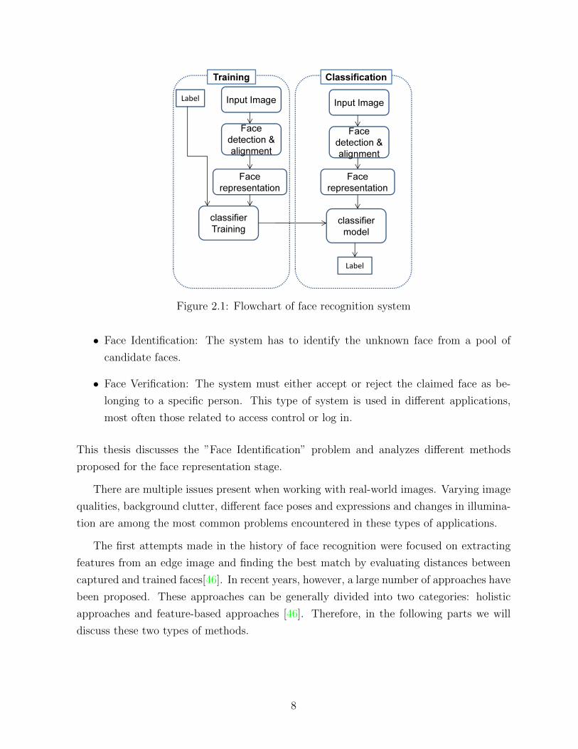
2.1 Flowchart of face recognition system . . . . . . . . . . . . . . . . . . . . . 8
3.1 The Canny edge detector . . . . . . . . . . . . . . . . . . . . . . . . . . . . 18
3.2 The Sobel edge detection. (a) Sample faces, (b) Detected edges along x
direction, (c) Detected edges along y direction, (d) Detected edges’ magnitude 19
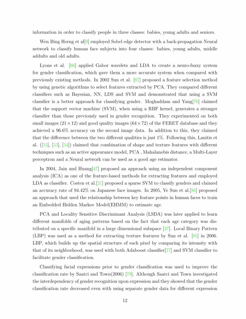
3.3 The 2-D Laplacian of Gaussian (LoG) function . . . . . . . . . . . . . . . . 21
3.4 The Laplacian edge detector . . . . . . . . . . . . . . . . . . . . . . . . . . 21
3.5 The eigenfaces corresponding to the sample faces . . . . . . . . . . . . . . 26
3.6 The fisherfaces corresponding to the sample faces . . . . . . . . . . . . . . 30
3.7 The LBPH descriptor . . . . . . . . . . . . . . . . . . . . . . . . . . . . . . 31
3.8 Examples of different texture structures detected by the LBP method (black
circles represent of ones’ ”1”, and white circles correspond to zeros ”0”) . . 33
3.9 43 sampling patterns used in FREAK method . . . . . . . . . . . . . . . . 35
3.10 Framework of Block-Based bag of Words(BBoW) . . . . . . . . . . . . . . 37
3.11 Sample faces in FERET database . . . . . . . . . . . . . . . . . . . . . . . 42
3.12 Collected LFW database . . . . . . . . . . . . . . . . . . . . . . . . . . . . 43
ix

3.13 Performance evaluation results of the Bag-of-Words method over uLBP fea-
tures with different number of words , gridding schemes and distances be-
tween pixels to extract descriptors . . . . . . . . . . . . . . . . . . . . . . . 51
3.14 Performance evaluation results of the Bag-of-Words method with 50 un-
known faces with different threshold and number of regions . . . . . . . . . 52
4.1 The flowchart of a gender and age recognition application . . . . . . . . . . 54
4.2 Representation of the real part of 40 Gabor filters . . . . . . . . . . . . . . 58
4.3 Color Histogram descriptor . . . . . . . . . . . . . . . . . . . . . . . . . . . 60
4.4 Illustration of levels 2, 1, and 0 split of an image . . . . . . . . . . . . . . . 61
4.5 The CLR-LBP descriptor . . . . . . . . . . . . . . . . . . . . . . . . . . . . 62
4.6 The first seven texture features selected by Ullman feature selection tech-
nique to classify gender subjects . . . . . . . . . . . . . . . . . . . . . . . . 64
4.7 The first seven texture features selected by Ullman feature selection tech-
nique to classify age subjects . . . . . . . . . . . . . . . . . . . . . . . . . . 65
4.8 The first seven shape features selected by Ullman feature selection technique
to classify age subjects . . . . . . . . . . . . . . . . . . . . . . . . . . . . . 65
4.9 Support vector Machine schema . . . . . . . . . . . . . . . . . . . . . . . . 66
4.10 Effect of the number of features selected . . . . . . . . . . . . . . . . . . . 75
x

Nomenclature
Abbreviations
BBoW Block-based Bag of Words
BoW Bag-of-Words
CBP Centralized Binary Pattern
CENTRIST CENsus Transform histogram
CGGH Centralized Gabor Gradient Histogram
CH Color Histogram
CLR-LBP Color-based Local Binary Pattern
DCT Discrete Cosine Transform
DWT Discrete Wavelet Transform
EHMM Embedded Hidden Markov Model
FERET The Facial Recognition Technology
FREAK Fast Retina Keypoint
HSV Hue-Saturation-Value
ICA Independent Component Analysis
LBP Local Binary Pattern
LBPH Local Binary Pattern Histogram
LDA Linear Discriminant Analysis
LDS Limited Discrepancy Search
LoG Laplacian of Gaussian
LSDA Locality Sensitive Discriminant Analysis
NN Neural Networks
PCA Principal Component Analysis
RBF Radial Basis Function
RGB Red-Green-Blue
SIFT Scale-Invariant Feature Transform
xi

SVM Support Vector Machine
SVR Support Vector Regression
ULBP Uniform Local Binary Pattern
WLD Weber Local Descriptor
xii

Chapter 1
Introduction
The field of face processing is growing at an exponential rate, covering many tech-
nical areas such as image processing, surveillance and security, telecommunication and
human-computer interaction. The world-wide range of commercial and law enforcement
applications are a sign of its huge economic significance. The demand to build an auto-
matic system to process face objects and extract the most useful information from this
biometric feature leads to the necessity of overcoming some difficulties.
In this thesis, two separate problems are studied: face recognition and estimating the
corresponding age and gender of face objects. Constructing applications to identify a
person from their face and extract their age and gender information is a challenging task
because of the necessity of creating a general model that works for all human subjects. As
each person has his/her own innate face distinctive characteristics that vary in a subtle way
from person to person, proposing a framework that extracts useful features to discriminate
between faces requires in-depth studies of human face objects.
Processing human faces requires considering many aspects. One such aspect is to
analyze face structure and determine the exact location of face elements, such as eyes,
noses, mouths, eyebrows, lips and cheeks. Another is the extraction of relevant information
from these detected elements which can provide us with useful information regarding the
identity, age, ethnicity and gender of a person.
While face recognition has been a very active field of research in the recent decades,
recognizing the age and gender from a face image has been more recently studied.
1

1.1 Motivation
Face, age and gender recognition has long been recognized as an important module for
many computer vision applications such as human-robot interaction, visual surveillance
and passive demographic data collections. Identifying persons to allow them access to
or control of facilities, tools and information are amongst the most common applications
of face recognition. As an example, facial recognition technology is currently being used
by hotels and casinos to identify a blacklisted of individual. Unlocking software on mobile
devices is another application that is developed and is available in Android Market (Visidon
Applock) to allow the owner to secure applications. Similar applications is integrated into
the iPhoto application for Macintosh, to let users organize and label their collections.
Employing facial recognition instead of fingerprint recognition systems is another system
which is being used for collecting the information regarding employee attendance and
presence at work.
The objective of our research project is designing a framework which will be of low
complexity such that it could be integrated into an embedded low power architecture.
In addition to the face recognition, the growing interest of the advertising industry,
which seeks to launch demographic-specific marketing and targeted advertisements in pub-
lic places is gaining more and more attention from researchers, who find themselves focusing
on the issue of age and gender recognition. The objective of our research project is to ex-
tract demographic information of human subjects who are in front of smart TV displays,
and deciding on the content to display for the audience and viewers based on the extracted
information and environment.
Considerable amounts of studies conducted in the field of face processing have provided
powerful and robust visual descriptors. Different visual descriptors regarding texture, shape
and color information have been proposed in order to provide more compact representations
for face objects. However, the challenge still remains to identify the ideal feature extraction
method. While powerful new feature extractors have been proposed, they still cannot be
applied to the real world applications because of their tendency to struggle to recognize
faces that have been subject to minor variations. Differing image qualities, background
clutter, different poses, changing facial expressions and varying levels of lighting are among
the difficulties that these applications often encounter. In addition to this, collecting
a good set of face images for building face models pose another problem. Designing a
framework capable of recognition performances similar to the ones of humans requires a
rich set of training images. For example, if we train a gender model with a set of faces
2

exclusively collected from Western people, it would not perform very well when tested on
other ethnicity groups such as Asian people.
1.2 Problem Description
The objective of this thesis is to propose a methodology for the automatic recognition of
facial/pattern occurrences from sample images captured in real time. Thus, two separate
problems will be studied: face recognition and determining the corresponding age and
gender of face objects. The common procedure for these two problems has been shown in
Figure 1.1.
Face &
Landmark
Detection
Face
Alignment &
Cropping
Face
Representation
Recognition /
Classification
Model
{a1, a
2, a
3, …, a
n-1, a
n}
Identity
Male/Female
Teenager/Adult/Senior
Figure 1.1: Main program flow diagram
1.2.1 Face Recognition
Face recognition is an interesting sub-area in the field of object recognition and can be
defined as identifying or verifying human subjects in various scenes from a digital image or
a video source. Human beings can recognize and identify faces learned during their lifetime
even after years of separation. Thus, the subject of majority of studies in face processing
is proposing a model that can recognize faces to a level similar to the average human’s
capacity [101].
While the currently existing face recognition systems obtained good results on face
images captured in a controlled environment, they are still far from being capable of ad-
3

equately adapting to uncontrolled situations. Proposing a system that can adapt itself
well to real-world applications and scenarios requires overcoming a number of difficulties.
Of these difficulties, we can mention face pose variation, changes in expression, lightning
conditions, clothing, hairstyle, makeup, background clutter, scaling, rotation, etc.
1.2.2 Age and Gender Recognition
Determining the age and gender of individuals from a live camera has many applications
in the world of advertising. When a frame is captured, a face detection technique is
employed to detect the face object. After detecting and aligning the face, the information
allowing for greater facial discrimination is extracted and these data are then used to
recognize the face’s age and gender category.
This thesis aims at increasing the performance of face processing techniques in recog-
nizing certain demographics (age and gender) from a face image. This information can
then be used to display targeted advertisements to individuals viewing smart TV displays.
1.3 Contribution
This thesis has two main contributions: an approach for face recognition, and a frame-
work for age and gender classification.
We have developed a face recognition framework that can be applied to real-world con-
ditions. After investigating different approaches, we have adopted a bag-of-words structure
[82] for face recognition by incorporating face-related features into it. We evaluated this
structure on a challenging dataset containing sample images featuring a variety of poses,
levels of illumination, backgrounds, expressions, clothing, hairstyles, cosmetics, etc. Figure
1.2 illustrates the face recognition application based on the proposed structure:
4

Figure 1.2: Example of the recognition provided by the proposed face recognition frame-work under different amount of illumination and occlusion
In addition to this, we propose a novel framework for gender and age classification that
facilitates the integration of multiple feature types and, in doing so, takes advantage of var-
ious sources of visual information. Furthermore, in the proposed method, only the regions
that can best separate face images of different demographic classes (with respect to age
and gender) contribute to the face representations, which in turn improves the classifica-
tion and recognition accuracies. Experiments performed on a challenging publicly available
database validate the effectiveness of our proposed solution and show its superiority over
the existing state-of-the-art methods. Figure 1.3 illustrates the age and gender recognition
application based on our proposed method.
Figure 1.3: Example of the prediction provided by the proposed age and gender recognitionframework
Our proposed method for age and gender recognition has been accepted in the Inter-
national Conference on Image Processing (ICIP) [30].
5

1.4 Thesis Outline
This thesis is divided into two parts, one for each contribution of the thesis. In Chapter
2, we review some previously proposed ideas related to our research. In Chapter 3, we
investigate different methods for face recognition. We first review well-known approaches
and later compare them in order to determine the most accurate ones. Finally, an extensive
experimentation was carried out in order to determine the optimal value for the parameters
of our proposed face recognition approach when analyzing different real-world conditions.
Chapter 4 discusses the problem of age and gender recognition. We first review existing
popular descriptors for face representation. Then, we explain the functioning of our novel
feature selection-based approach, which aims at facilitating the integration of multiple
feature types. We end with a presentation and explanation of the results by our proposed
method.
Finally, in Chapter 5, we summarize the contributions of this thesis and indicate possible
future areas of development.
6

Chapter 2
Literature Review
Face processing has long been recognized as an important module for many computer
vision applications. Face recognition, and the classification of the age and gender of face
objects are two interesting field of research in this area. With such a face analysis compo-
nent, it becomes possible to identify a person in order to allow access to private facilities or
to display targeted information in advertising based on demographic category of individu-
als in public places. In this chapter we provide a brief review of some of existing methods
in face, gender and age recognition and discuss their strengths and weaknesses.
2.1 Face Recognition
Face recognition has received significant attention in recent years. In spite of the
progresses in this field, there are still several challenges associated with applying face
recognition to real world situations. Among the most important applications in which face
recognition plays a key role, we can mention access control, law enforcement and video
surveillance [101].
When given an image to process, the face recognition system detects a human subject
through face detection techniques and the face region is segmented from the image. The
next stage is then to identify the facial features of the face in order to align it in a canonical
way. A face representation is then extracted from the face. Then, the face representation
is fed to the classification model to find the face in our pre-trained database, which best
corresponds to the extracted face representation. In short, the entire procedure can be
explained through the flowchart of Figure 2.1.
Face recognition has traditionally been divided into the following two different problems:
7
Input Image
Face
detection &
alignment
Face
representation
classifier
Training
Label
Training
Input Image
Face
detection &
alignment
classifier
model
Label
Classification
Face
representation
Figure 2.1: Flowchart of face recognition system
• Face Identification: The system has to identify the unknown face from a pool of
candidate faces.
• Face Verification: The system must either accept or reject the claimed face as be-
longing to a specific person. This type of system is used in different applications,
most often those related to access control or log in.
This thesis discusses the ”Face Identification” problem and analyzes different methods
proposed for the face representation stage.
There are multiple issues present when working with real-world images. Varying image
qualities, background clutter, different face poses and expressions and changes in illumina-
tion are among the most common problems encountered in these types of applications.
The first attempts made in the history of face recognition were focused on extracting
features from an edge image and finding the best match by evaluating distances between
captured and trained faces[46]. In recent years, however, a large number of approaches have
been proposed. These approaches can be generally divided into two categories: holistic
approaches and feature-based approaches [46]. Therefore, in the following parts we will
discuss these two types of methods.
8

2.1.1 Holistic Approaches
Holistic approaches developed for face recognition are based on processing the whole
face and then representing it in a generic form. These methods extract features from a
face without considering from which face areas they hail. As the dimension of each image
is quite large, processing the whole face is difficult in practice. Because of this, dimension
reduction approaches are applied in conjunction with holistic techniques.
Among the large amount of proposed algorithms in holistic approaches we can men-
tion: Principal Component Analysis (PCA) [90], Linear Discriminant Analysis (LDA)
[67], Discrete Wavelet Transform [4], Discrete Cosine Transform (DCT) [39], and Bayesian
Intra-personal and Extra-personal Classifier [95].
PCA, as proposed by K. Pearson [74] and H. Hotelling [40], extracts a set of orthogonal
basis vectors from the training data and then represents each data vector by a weighted
sum of the extracted basis. This method has also been applied to face images by M.
Turk in [90] where PCA was applied as a dimension reduction technique to preserve the
most significant basis (called eigenfaces). Follwoing this, each face was represented in the
subspace spanned by these bases. They proposed a near-real-time application based on
this method and experimented on a set of 2500 face images collected under controlled
conditions [90].
LDA, invented by R.A. Fisher [67], is a method for dimension reduction and data clas-
sification which relies on mapping data to a new space within which each class, data have
minimum variance and the maximum distance between classes. This method was applied
to face recognition by K. Etemad and R. Chellappa [29] on a set of features extracted by
Wavelet Transform and experimented on a database provided by The Olivetti Research
Laboratory (ORL) and containing 40 different subjects featuring a variety of changes in
illumination, facial expression and facial details (glasses or no glasses) as well as some side
movements.
Discrete Wavelet Transform (DWT) is another holistic techniques and is based on
the discrete sampling wavelet transform. In its basic format, DWT is used by a 2-D
wavelet decomposition, which applies a 1-D transformation in X-direction and another Y-
direction. This transformation generates four sub-images, which correspond to the different
frequencies in each direction (High-High, High-Low, Low-High, Low-Low). Following this,
the feature vector is constructed by using information of the Low-Low sub-image which is
then employed for finding the match within trained faces ([76], [80]).
Discrete Cosine transform is a popular method in image compression and is another
9

method in the category of holistic transform. This method applies a 2-D DCT on image
and then codes the entropy of the quantized samples to get the result. DCT is a strong
technique for ”energy compaction” and was applied to the process of face recognition by
M. J. Er et al. [39], who carried out their experiments on three databases : 1) ORL, 2)
The FERET database and 3) The Yale database.
The Bayesian Intra-personal and Extra-personal Classifier method exploits the fact
that two different image classes span subspaces with Gaussian distribution properties
[89]. Moghaddam and Pentland [69] showed that these subspaces (called extra-personal
and intra-personal subspaces) cooperated with similarity measurements computed by a
Bayesian rule that gives the probability on how likely a vector belongs to a specific sub-
space [69].
2.1.2 Feature Based Approaches
These approaches rely on the fact that all human subjects share the same fundamental
structures and the only true difference is the geometric relations between said structures.
Therefore, feature-based methods will, at first, extract facial features like eyes, nose, mouth,
eyebrows, etc and then extract the existing relationship between these facial features. Of
the common algorithms employed for this purpose, we can mention deformable templates,
the Hough Transform method and Elastic Bunch Graph Matching.
The deformable templates method is based on the idea that a family of objects can
be represented by deformations of a basic ideal template. This notion is what makes this
technique more robust against the different scales and positions that a face object can
adopt as well as changes in illumination [98]. This method finds sets of features by using
spatial relations and prior knowledge of the general layout of a face to build a vector of
features, which is then used to represent and recognize faces.
The basic Hough Transform method has been applied to detect straight lines [41] and
was later extended by R. Duda and P. Hart[26] so as to be able to compute shape analysis
and identify arbitrary shapes. This approach was applied for the purposes of face recog-
nition in [41] and proved its robustness against various noises. It also has high level of
efficiency in terms of its memory usage.
One of the other feature-based methods frequently used is Elastic Bunch Graph Match-
ing. This approach builds a graph based on the face structure, that connects the detected
facial features, such as eyes, nose, etc. The edges represent the similarity distance between
the nodes. Wiskott et al. [95] used Elastic Bunch Graph Matching in face recognition by
10

constructing each node with Gabor filter results and utilizing the edges to describe the
geometrical properties of each face.
In this section, we presented a short overview of the two main categories in face recogni-
tion. Holistic approaches process the entire face and extract a global representation, which
is then be fed to the recognition stage system. Feature-based methods directly identify
facial features and employ the spatial structures between them to identify the face. Al-
though processing each facial structure separately creates a system that is robust against
position variation, lighting condition changes and noise, in the last few decades, holistic
approaches have attracted more attention from researchers specializing in the field of face
processing [101]. In our thesis we will look over different methods in these categories to
identify which ones offer optimal performances in the real world.
2.2 Age and Gender Recognition
Age and gender recognition is an important modules for many computer vision appli-
cations such as human-robot interaction, visual surveillance and passive demographic data
collections. More recently, the advertising industry’s growing interest in the launching
demographic-specific marketing and targeted advertisements in public places has attracted
the attention of more and more researchers specialized in the field of computer vision. In
this section, we will take a brief look at the different techniques proposed in the field of
age and gender recognition. A detailed survey of studies on age and gender recognition
can also found [71], [68])
Among the early algorithms in the field of age and gender recognition, Cottrel and Met-
calfe [22] extracted whole-face features called Holons, which were fed into a back propaga-
tion network model to classify males and females. Golomb et al. [36] proposed ”SEXNET”
Neural Network model for gender recognition. This network compresses faces using faces’
raw pixels and then estimates their sex in subsequent layers of their proposed network.
In 1995, Brunelli and Poggio [11] achieved a 79% recognition rate for gender by using the
HyperBF network on a set of geometrical features extracted from faces and, shortly after,
Abdi et al.[2] employed the RBF network and achieved a 90% recognition rate on data
preprocessed by PCA. In 1997, wavelet components (jets) were exploited by Wiskott et
al.[96] in order to describe face features and build Elastic Bunch Graph models. In 1999,
Kwon and Lobo[52] proposed a method for age classification that first extracted specific
features of the face elements such as eyes, noses, mouths and chins. It then compute the
ratios estimated between the top of sides of the head before, finally, processing skin wrinkle
11
information in order to classify people in three classes: babies, young adults and seniors.
Wen Bing Horng et al[9] employed Sobel edge detector with a back-propagation Neural
network to classify human face subjects into four classes: babies, young adults, middle
addults and old adults.
Lyons et al. [66] applied Gabor wavelets and LDA to create a neuro-fuzzy system
for gender classification, which gave them a more accurate system when compared with
previously existing methods. In 2002 Sun et al. [87] proposed a feature selection method
by using genetic algorithms to select features extracted by PCA. They compared different
classifiers such as Bayesian, NN, LDS and SVM and demonstrated that using a SVM
classifier is a better approach for classifying gender. Moghaddam and Yang[70] claimed
that the support vector machine (SVM), when using a RBF kernel, generates a stronger
classifier than those previously used in gender recognition. They experimented on both
small images (21×12) and good quality images (64×72) of the FERET database and they
achieved a 96.6% accuracy on the second image data. In addition to this, they claimed
that the difference between the two different qualities is just 1%. Following this, Lanitis et
al. ([55], [53], [54]) claimed that combination of shape and texture features with different
techniques such as an active appearance model, PCA , Mahalanobis distance, a Multi-Layer
perceptron and a Neural network can be used as a good age estimator.
In 2004, Jain and Huang[47] proposed an approach using an independent component
analysis (ICA) as one of the feature-based methods for extracting features and employed
LDA as classifier. Costen et al.[21] proposed a sparse SVM to classify genders and claimed
an accuracy rate of 94.42% on Japanese face images. In 2005, Ye Sun et al.[86] proposed
an approach that used the relationship between key feature points in human faces to train
an Embedded Hidden Markov Model(EHMM) to estimate age.
PCA and Locality Sensitive Discriminant Analysis (LSDA) was later applied to learn
different manifolds of aging patterns based on the fact that each age category was dis-
tributed on a specific manifold in a large dimensional subspace [37]. Local Binary Pattern
(LBP) was used as a method for extracting texture features by Sun et al. [85] in 2006.
LBP, which builds up the spatial structure of each pixel by comparing its intensity with
that of its neighborhood, was used with both Adaboost classifier[77] and SVM classifier to
facilitate gender classification.
Classifying facial expressions prior to gender classification was used to improve the
classification rate by Saatci and Town(2006) [79]. Although Saatci and Town investigated
the interdependency of gender recognition upon expression and they showed that the gender
classification rate decreased even with using separate gender data for different expression
12

classes. In 2007, a color descriptor relying on the construction of histograms with 4 bins
per color channel in the RGB color space was proposed for gender classification [45]. The
fusion approach, 2D PCA and the centralized Gabor gradient histogram (CGGH) were
other methods that were employed in feature extraction [Lu and shi (2009)[65], Len Bui
(2010)[12], Xiaofeng Fu(2010)[32]]. Xiaofeng Fu[32] combined CBP and Gabor gradient
magnitudes to extract more discriminative features at multiple scales and orientation[45].
By feeding these features into a nearest center-based neighbor classifier, they achieved a
96.56% accuracy rate on FERET and a 95.25% accuracy rate on CAS-PEAL. Meanwhile,
in 2010, Guo-Shiang Lin and Yi-Jie Zhao [60] proposed a color-based approach on SVM
for gender classification. In 2011, compressive sensing framework was applied by Duan-Yu
Chen and Po-Chiang Hsieh [17] to represent face images in a sparse frequency domain.
They extracted two feature sets for each gender; the first set presenting features that
are common between all the images in corresponding gender classes and the other one
representing each individual face in that class. Ihsan Ullah et al. (2012) [91] used spatial
WLD as a texture descriptor for gender recognition. They divided the image into a number
of blocks, calculated the WLD descriptor for each block and concatenated them.
In 2013, Chen, Y. et al.[18] introduced a new method based on subspace learning that
operates as a set of constrained optimization problems to characterize age-related features.
By employing semi-supervised learning techniques they applied the Support Vector Regres-
sion(SVR) methods onto the features to create an age estimators model. Juan E. Tapia
and Claudio A. Perez (2013)[88] proposed a method, which uses feature selection based on
mutual information and the fusion of intensity, shape and texture features to classify gen-
der classes. They then calculated LBP features with different radial and spatial scales, and
then selected features using mutual information. They tested three different techniques to
measure mutual information: minimum redundancy and maximum relevance[25], normal-
ized mutual information[28], and conditional mutual information-based [19].
Therefore, we can summarize that the most of the efforts made to optimize in gender
and age recognition from a face object attempt to best represent the face object. While
some methods choose to use raw pixels (e.g., [2], [3] and [4]) without any modification, the
majority of the existing methods use local visual descriptors to produce stronger and, often,
more compact representations of face images. Examples of visual information commonly
used for age and/or gender recognition are texture information (e.g., used in [55],[53],[54],
[85], [91], [3]), shape information (e.g., used in [88], [27], [13]) and color information (e.g.,
used in [60] and [45]). In these methods, local descriptors are extracted from a dense regular
grid placed over the entire image and the face representation is built by concatenating these
extracted descriptors into a single vector. A key issue in this framework is to determine the
13

optimal grid parameters (e.g., spacing, size, number of grids in multi-resolution/pyramid
approaches, etc.). Dago-Casas et al. [24] proposed to use raw pixels, Gabor jets and LBPs
on Gallaghers database for gender recognition. They reduced the size of extracted features
by using Principle Component Analysis and showed that, by using Gabor jets followed by
SVM high gender classification, a greater accuracy is obtained. While the aforementioned
methods for age and gender recognition used fixed settings and performed trial-and-error
to determine the right grid parameters, a better approach consists in using feature selec-
tion to allow only the most informative image regions (or grid cells) to contribute to the
face representation, i.e., those that can best separate face images that belong to different
demographic classes. This approach further facilitates the integration of different types
of descriptors (e.g., color based, shape based, texture based, etc.) and allow for more
compact representations by preventing redundant features from contributing to the face
representation.
2.3 Conclusion
This chapter has described different attempts that have been made in the fields of face,
gender and age recognition. The main issue addressed by these methods is how to best
represent a face in such a way that it will be most efficiently identified. It is in this vein
that we will go over different techniques used to represent faces and to try to come up with
a generic algorithm that can be applied to solve our problem: accurate face representation
and recognition.
14
Chapter 3
Face Recognition
The development of applications to extract the distinctive features from face images
has been the motivation behind the majority of studies in the field of face processing.
These studies proceed by detecting a face and extracting a compact representation from
it. As face processing research has progressed, increasingly complex challenges have been
encountered, and new techniques have been proposed to provide accurate and robust ways
of solving these problems.
Although there are many different branches in the field of face processing, face recogni-
tion is an essential component. In general, solving this problem requires overcoming certain
difficulties, such as differing image qualities, background clutter, poses, facial expressions,
and varying levels of lighting. This chapter summarizes some popular methods for facial
recognition and propose a face recognition approach that is robust, simple, and efficient to
use when compared to other existing methods.
While some methods choose to extract features from raw pixels, others first employ pre-
processing techniques to reduce the impact of changing illumination and contrast before
extracting the facial features. Section 3.1 presents some common edge detectors that can
be used to this end. Then, section 3.2 highlights the two classic techniques that have
been applied for the global representation of a face image. Section 3.3 is dedicated to
popular feature-based methods, in particular LBPH, SIFT, BRIEF, and FREAK. Section
3.4 describes the Block-based Bag-of-Words method representation method. Section 3.5
presents a matching strategy to effectively establish face matches. Finally, experimental
results are reported in section 3.6. We introduce two datasets against which we benchmark
the previously mentioned methods.
15

3.1 Edge Detection Techniques
As mentioned in the previous chapter, one of the main steps of face processing is face
representation, which requires extracting the most relevant information to characterize a
face. Although edge detection operators are not categorized as powerful descriptors, com-
bining them with other methods can lead to the removal of noise artifacts while preserving
the useful face features.
Generally, edge detection consists in computing the gradient magnitude of an image.
Edges localize sudden changes in intensities of color or illumination in images. An image
gradient can be computed by applying convolution masks on the image. In this section
we describe the Canny edge detector as well as the Sobel and Laplacian edge detection
techniques. The objective of employing these techniques is to limit the impact of intensity
variation in the face image, thus allowing for more robust descriptors to be extracted.
3.1.1 Canny Edge Detector
The Canny Edge detector is one of the most common edge detection techniques. This
technique proceeds as follows:
• First, a blurring operation, such as a Gaussian filter, is applied to the image to
suppress input noises and distinguish between the simple edges and meaningful edges,
such as the contour of objects.
To smooth the image and suppress unnecessary texture edges, the following Gaussian
filter can be applied:
G(x, y) =1
2πσ2e−
x2+y2
2σ2 (3.1)
where σ value controls the smoothing level.
• Next, the gradient magnitude and direction is computed by evaluating the gradient
in x and y directions:
M = |√G2x +G2
y| Where Gx =∂Is∂x
and Gy =∂Is∂y
θ = arctan(Gy
Gx
)
(3.2)
Then the angle computed for θ is rounded to four directions: 0◦, 45◦, 90◦, and 135◦.
Finally, nonmaxima suppression is applied to the computed gradient magnitude.
16

In this procedure, edges which have the large gradient’s magnitude are preserved.
Additionally, broad ridges are thinned and all other edges that belong to smooth
textures on the ridge are suppressed. For this purpose, we seek local maxima by
checking the 3× 3 region around each pixel, taking into account its orientation [15]:
1) If θr(x, y) = 0, then we compare the M(x, y) value with M(x − 1, y) and
M(x+ 1, y)
2) If θr(x, y) = 45, then we compare the M(x, y) value with M(x− 1, y − 1) and
M(x+ 1, y + 1)
3) If θr(x, y) = 90, then we compare the M(x, y) value with M(x, y − 1) and
M(x, y + 1)
4) If θr(x, y) = 135, then we compare the M(x, y) value with M(x− 1, y+ 1) and
M(x+ 1, y − 1)
In the aforementioned situations, if M(x, y) has a large value, it would be kept as an
edge. Otherwise, it would be removed as it is not a local maxima.
At this stage, the algorithm suggests to employ double thresholding techniques to
detect and link edges [15]. By using two levels of thresholding, more meaningful
edges are obtained. Applying a high value threshold will give us edges corresponding
to real contours that are then linked using edges detected at a lower threshold.
Figure 3.1 illustrates the result of applying a Canny edge detector on the face images.
17

Figure 3.1: The Canny edge detector
3.1.2 Sobel Edge Detector
Sobel, as proposed by Irwin Sobel [84], is another popular technique for edge extraction.
This method, which approximates the 2-D spatial gradient of images, has been combined
with several algorithms for the purpose of face recognition (e.g., [58], [61], and [100]). The
basic version of this filter convolves two 3× 3 kernel filters with a grayscale image. These
two filters, Gx and Gy, which correspond to horizontal and vertical derivative masks are
defined as follows [84]:
Gx =
−1 0 +1
−2 0 +2
−1 0 +1
Gy =
+1 +2 +1
0 0 0
−1 −2 −1
(3.3)
And the gradient magnitude is computed as:
θ = arctan(GY
GX
)
G =√G2X +G2
Y
(3.4)
where Gx and Gy are the computed gradient values of a pixel in location (x, y).
Figure 3.2 shows the result of applying Gx and Gy on an image and G as the corre-
sponding image’s magnitude:
18

(a) (b) (c) (d)
Figure 3.2: The Sobel edge detection. (a) Sample faces, (b) Detected edges along x direc-tion, (c) Detected edges along y direction, (d) Detected edges’ magnitude
3.1.3 Laplacian Edge Detector
The next technique is the Laplacian edge detector. Unlike the Sobel technique, which
finds intensity variations by observing the first derivation of images, the Laplacian method
uses the second derivation of images. Since intensity changes appear as the maximum or
minimum points in the first derivation of the image, the second derivative crosses the zero
axis in these critical points. On this basis, the 2-D Laplace operator has been defined as
follows:
52 = 5.5 = (∂
∂x~i+
∂
∂y~j).(
∂
∂x~i+
∂
∂y~j) = (
∂2
∂x2)���>
1(~i.~i) + (
∂2
∂y2)���>
1(~j~j) + (
∂
∂x
∂
∂y)���>
0(~i.~j) + (
∂
∂x
∂
∂y)���>
0(~j.~i)
=∂2
∂x2+
∂2
∂y2
(3.5)
This operator can be utilized by employing a filter mask. We first calculate an approx-
19

imation kernel for second derivation and then convolve it into the image. For this purpose
we can create filters with different sizes by manipulating partial sums of the Taylor series:
f(x+ h) = f(x) +h1
1!f(x) +
h2
2!f ′′(x) +
h3
3!f ′′′(x) +
h4
4!f ′′′′(x) + · · ·
f(x− h) = f(x)− h1
1!+h2
2!f ′′(x)− h3
3!f ′′′(x) +
h4
4!f ′′′′(x) + · · ·
f(x+ h) + f(x− h) = 2f(x) + 2h2
2!f ′′(x) + 2
h4
4!f ′′′′(x) + h6c
f ′′(x) =f(x+ h)− 2f(x) + f(x− h)− 2h
4
4! f′′′′(x)− h6c
h2=f(x+ h)− 2f(x) + f(x− h)
h2+ h2c′
So by setting h = 1:∂2I(x, y)
∂x2≈ f(x+ 1, y)− 2f(x, y) + f(x− 1, y)
and similarly∂2I(x, y)
∂y2≈ f(x, y + 1)− 2f(x, y) + f(x, y − 1)
as 52 I(x, y) =∂2I
∂x2+∂2I
∂y2
=
0 0 0
f(x− 1, y) −2f(x, y) f(x− 1, y)
0 0 0
+
0 f(x, y − 1) 0
0 −2f(x, y) 0
0 f(x, y + 1) 0
=
0 f(x, y − 1) 0
f(x− 1, y) −4f(x, y) f(x− 1, y)
0 f(x, y + 1) 0
(3.6)
As such, kernel L1 =
0 1 0
1 −4 1
0 1 0
is one of the kernels that can be used as an approx-
imation for the second derivative. Other common forms of 3 × 3 kernels that have been
derived in a similar way have been provided as follows:
L2 =
2 −1 2
−1 −4 −1
2 −1 2
L3 =
1 1 1
1 −8 1
1 1 1
Although kernels in other sizes can be employed to make this approximation (3.5) more
accurate, all of them are extremely sensitive to noise due to their nature. The simple
solution to overcome this problem is to apply an additional Gaussian filter to suppress the
noise. By the associative property of convolution, we can write:
52 [G(x, y) ∗ I(x, y)] = 52[G(x, y)] ∗ I(x, y) (3.7)
20
where the term G(x, y) represents the Gaussian filter and52[G(x, y)] is the denoted Lapla-
cian of Gaussian (LoG(x, y)). LoG is computed by taking the derivative which is equal
to:
LoG(x, y) = − 1
πσ4(1− x2 + y2
2σ2)e−
x2+y2
2σ2 (3.8)
As demonstrated above, a mask filter can be used in different scales of σ, as is the case in
the following figure, which corresponds to LoG with σ = 1.5:
Figure 3.3: The 2-D Laplacian of Gaussian (LoG) function
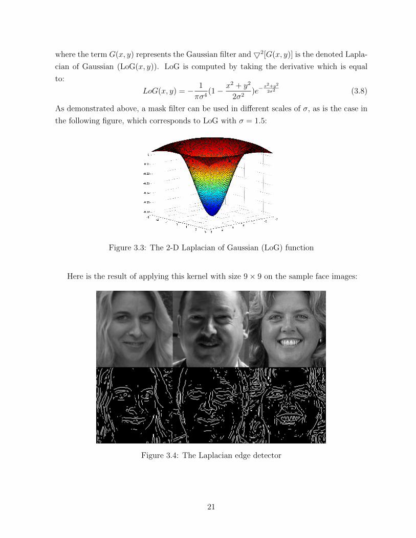
Here is the result of applying this kernel with size 9× 9 on the sample face images:
Figure 3.4: The Laplacian edge detector
21

3.2 Global Representation
As discussed earlier, global representation for face recognition is based on processing
the whole face and then representing it in a generic form. These methods extract features
from a face without considering the areas of the face from which these come. The objective
of these approaches is to reduce the dimensionality of feature data extracted from the face
image, thus allowing for more distinctive data to be used to represent a face. In this
section, two classical approaches, PCA and LDA, will be discussed.
3.2.1 Principle Component Analysis (PCA)
Principle Component Analysis (PCA), as proposed by Karl Pearson [74], is one of the
more commonly used statistical approaches to dimensional reduction and data classifica-
tion. This method computes the transformation of a set of correlated variables into a
set of linearly uncorrelated vectors called principal components. The relevance of this
transformation lies in the fact that the number of required components to represent data
is less than the full dimension of its original one. This method, also known as the dis-
crete Karhunen-Leove transform, represents a stochastic process as an infinite linear
combination of orthogonal basis vectors.
In the Karhunen-Leove method ([49], [1]), a signal (X) is assumed to be made of N ×1
random vector with an auto-correlation defined as R = E[XXH ]. Employing the Cholesky
factorization method, we can write the matrix R as R = UΛUH , where the columns of U
correspond to the normalized eigen-vectors of R. Then, our data can be transformed to
the zero-mean random vector Y with uncorrelated components:
E[Y Y H ] = Λ (3.9)
Furthermore, our original data (X) can be synthesized by employing a linear combination
of the uncorrelated random variable Y as follows:
X = UX =N∑i=1
uiYi (3.10)
However, as mentioned previously, the Y vectors are a set of orthogonal vectors (which are
basically the eigen-vectors of the correlation matrix R), and this representation is called
the Karhunen-Loeve expansion of X.
22

The aim is to find an approximate representation of a signal X requiring as few com-
ponents as possible based on the approximation:
x = Kx (3.11)
where K is an N ×N matrix with a rank of less than N . This representation of X can be
determined using a mean-squared error minimization approach. Such an approximation
is called a low-rank approximation. By considering that λ1, λ2, · · · , λN and x1, x2, · · · , xNcorrespond to the set of eigen-values and eigen-vectors of the auto-correlation matrix R,
the mean-squared error can be expressed as follows:
e2(K) = E[(X − X)H(X − X)] = tr(E[(X − X)(X − X)H ]) = tr(E[(X −KX)(X −KX)H ])
= tr(E[(I −K)XXH(I −K)H ]) = tr((I −K)R(I −K)H)
(3.12)
Then, by using orthogonal decomposition and assuming that K is Hermitian, we can write:
K =r∑i=1
µiuiuHi = UMrU
H (3.13)
where r is the new rank (r < N), U is a unitary matrix and Mr is equivalent to:
Mr =
µ1 0 0 0 0 · · · 0
0 µ2 0 0 0 · · · 0... 0
. . . 0 0 · · · 0
0 · · · 0 µr 0 · · · 0
0 · · · 0 0 0 · · · 0...
......
......
. . ....
0 · · · 0 0 0 0 0
(3.14)
As such, the error in equation 3.12 is expressed as follows:
e2(K) =r∑i=1
uHi Rui(1− µi)2 +N∑
i=r+1
uHi Rui (3.15)
It follows that in order to minimize 3.15 all values µ1, µ2, · · · , µr should be equated to one
(1) in the first term and those in the second term (∑m
i=r+1 uHi Rui) should be minimized.
As stated previously, ui corresponds to the i’th eigen-vector of R. Therefore, the rank-r
23

projection matrix K can be expressed as follows:
K =r∑i=1
uiuHi = UIrU
H (3.16)
where:
Ir =
1 0 0 0 0 · · · 0
0 1 0 0 0 · · · 0... 0
. . . 0 0 · · · 0
0 · · · 0 1 0 · · · 0
0 · · · 0 0 0 · · · 0...
......
......
. . ....
0 · · · 0 0 0 0 0
(3.17)
Based on this derivation, PCA tries to collect the principle components having the
highest variance. At each step, eigen-vectors corresponding to the largest principle com-
ponent are selected under the constraint of orthogonality to preceding components. When
the signal to process is a face image, these eigen-vectors are often referred to as eigen-faces.
The following section will describe how a set of eigen-faces is selected to represent a face
image.
Eigenfaces
A face image with size N × N can be considered as a vector of dimension N2. If
each pixel takes a value between 0 and 255, the face image lies on a large hypercube
with N2 dimensions where most of the points in the space does not correspond to any
face. Therefore, it can be assumed that face data in fact belongs to a lower dimensional
subspace. By employing PCA based on the Karhunen-Loeve algorithm, it is possible to
find the vectors that best account for the distribution of face data within this space.
Assuming that our training face images are represented by I1, I2, · · · , IM , the average
face vector can be easily expressed as follows:
Ψ =1
M
M∑i=1
Ii (3.18)
After subtracting the average face from all face images, we employ their covariance matrix
to compute the orthornormal vectors, ui, and extract the distribution of the training face
24

data:Φi = Ii −Ψ
C =1
M
M∑i=1
(Φi)(Φi)T =
1
MAAT
(3.19)
where A =[Φ1 Φ2 · · · ΦM
]and C is a N2×N2 matrix corresponding to the covariance
matrix. It is obvious that if the number of face images is less than the dimension of our
space (N2), a maximum of M − 1 eigen-values would be non-zero, and the rest of them
are not associated with meaningful eigen-vectors.
Afterwards, we have to compute the eigen-vectors of matrix C(AAT ):
AATvi = µiui (3.20)
Since AAT is a huge matrix, finding its eigen-vectors is not always practical. Thus, we go
over matrix ATA, which has the same eigen-values, and for which the eigen-vectors are
computed as follows:
ATAvi = λivi (3.21)
premultiplying both sides by A:
AATAvi = λiAvi ⇒ AAT (Avi) = λi(Avi) (3.22)
As vi, and ui are the eigen-vectors corresponding to ATA and AAT respectively, we have:
ui = Avi (3.23)
By preserving the r largest eigen-values, the size of each face representation will be reduced.
These eigen-vectors (ui) span a range of face images. Figure 3.5 shows eigen-faces extracted
from some face images.
25

Figure 3.5: The eigenfaces corresponding to the sample faces
Next we project a face image onto an eigenface component by the following mapping:
Ik = uTk (I −Ψ) k = 1, ..., r (3.24)
Finally, face representation is constructed in the eigenface’s space by concatenating all
computed components:
I =[I1, I2, · · · , Ir
](3.25)
This representation will be used next for classification, in finding the best match between
face classes. Each face class is calculated by obtaining the average over the results of the
eigen-face representation for all faces within it. In addition to this, a threshold, θk, is
assigned to each class to determine the maximum allowable distance between those faces.
This threshold is calculated based on all face data within that class.
One of the first and most prevalent ways to find the best match for a test image is to
compare the Euclidean distance between its extracted descriptor by PCA (Io) and the ones
extracted from the input set (Ik ∈ SM). It can be expressed as follows:
Ip = arg minIk∈SM
||(Io − Ik)|| (3.26)
where SM is the set of the face classes.
26

3.2.2 Linear Discriminant and Fisher Analysis
Another popular approach in pattern classification is the Linear Discriminant Analysis
(LDA) [67]. This method aims at finding the projection that best separates different
classes. For this purpose, LDA defines a measurement of separation between the classes:
J(µ) = |µ1 − µ2| (3.27)
where, µi = 1Ni
∑x∈Ci x and Ci represents class i.
Therefore, LDA aims to find an appropriate projection of y = W Tx, which will allow
the distance to become sufficiently large, as shown below:
J(w) = |W Tµ1 −W Tµ2| = |W T (µ1 − µ2)| (3.28)
Since this expansion simply considers the distance between the means of classes, and does
not provide any other information regarding the scattering of data in each class, it is not
always a good measurement of the distances between them. Consequently, Fisher [67]
proposed a measurement for two classes as follows:
J(w) =|W Tµ1 −W Tµ2|2
s12 + s1
2 (3.29)
where s12 and s2
2 are the parameters that correspond to the variability within class 1 (C1)
and class 2 (C2) after projection. As such, s12 + s1
2 measures the variability within the
two classes and is called the within-class scatter of the projected samples.
Fisher’s technique aims to maximize the function 3.29 by finding a projection in which
data from the same class are projected very close to one another, while data from different
27

classes are placed as far apart as possible. This projection can be found as follows:
J(w) =|W Tµ1 −W Tµ2|2
s12 + s1
2
|W Tµ1 −W Tµ2|2 = (W Tµ1 −W Tµ2)(WTµ1 −W Tµ2)
T = W T (µ1 − µ2)(µ1 − µ2)T︸ ︷︷ ︸SB
W = W TSBW
s12 + s1
2 =∑x∈C1
(W Tx−W Tµ1)2 +
∑x∈C2
(W Tx−W Tµ2)2
=∑x∈C1
W T (x− µ1)(x− µ1)T︸ ︷︷ ︸S1
W +∑x∈C2
W T (x− µ2)(x− µ2)T︸ ︷︷ ︸S2
W
= W TS1W +W TS2W = W T (S1 + S2)W = W T (SW )W
J(w) =|W Tµ1 −W Tµ2|2
s12 + s1
2 =W TSBW
W TSWW(3.30)
Where SB and SW are the between-class scatter and within-class scatter matrices of
the training data.
For finding the appropriate value of w that maximizes J(w), differentiation is applied
and set equal to zero:
∂
∂W(W TSBW
W TSWW) = 0
∂∂W
(WTAW )=2AW−−−−−−−−−−−→=
(W TSWW (2SBW )−W TSBW (2SWW ))
(W TSWW )2= 0
⇒ (W TSWW (2SBW )−W TSBW (2SWW )) = 0
Deviding by 2WTSWW :−−−−−−−−−−−−−−→ ((SBW )− 2wTSWW
W TSBW︸ ︷︷ ︸J(W )
(SWW )) = 0
⇒ SBW − J(W )SWW = 0As J(W ) is a scalar:−−−−−−−−−−−→ SBW = J(W )SWW
⇒ S−1W SBW = J(W )W
(3.31)
The final formula in 3.31, is an eigen-value equation and the maximum value for J(W ) is
equivalent to the largest eigen-value of S−1W SB, which is equivalent to:
J(W )max = S−1B (µ1 − µ2) (3.32)
28

To extend these formulas to multiple classes, our X, Y , and W are expressed as follows:
X =
x1(1) x2(1) · · · xM (1)
x1(2) x2(2) · · · xM (2)...
... · · ·...
x1(n) x2(n) · · · xM (n)
n×M
Y =
y1(1) y2(1) · · · yM (1)
y1(2) y2(2) · · · yM (2)...
... · · ·...
y1(M − 1) y2(M − 1) · · · yM (M − 1)
M−1×M
W = W TX W = [W1,W2, · · · ,WC−1]
(3.33)
Note that for M-classes, we have M − 1 projection vectors. Then SW and SB in equation
3.29 become:
SW =M∑i=1
SCi
SB =M∑i=1
Ni(µi − µ)2 where µ =1
N
∑∀x
x and µi =1
Ni
∑x∈Ci
x
where N = Number of all data and Ni = Number of data in class Ci
(3.34)
As shown above, unlike the PCA which maximizes the overall scatter, the LDA method
maximizes the ratio of between-classes to within-classes scatter. This method has been
applied to face recognition by Belhumeur et al. [7]. Based on their approach, LDA is being
applied to learn a class-specific transformation matrix (W ) that omits other information
regarding noise, such as illumination, leading to a basic improvement when compared to
the PCA approach. The use of the LDA, which uses the best facial features to separate
the persons in the training set, is dependent on the input set. If the system is trained
with the well-illuminated faces, it would not be a robust model to recognize faces in badly-
illuminated or unconstrained conditions.
Figure 3.6 shows the reconstruction of the projected face images using the Fisher-faces
technique:
29

Figure 3.6: The fisherfaces corresponding to the sample faces
3.3 Feature-Based Approaches
In contrast to the methods presented in the previous sub-sections, which treat the
whole image as a single vector. Feature-based approaches focus on extracting local features
related to edges, corners, and other structures within an image. Since these approaches
extract information by considering the important parts inside the image, they map better
to face recognition problems in comparison to global representation techniques. In this
section, we describe LBPH, SIFT, BRIEF and FREAK which are popular feature-based
approaches in face recognition.
3.3.1 Local Binary Patterns Histograms
Local Binary Pattern Histogram (LBPH) is one of the most powerful texture-encoding
descriptors. It extracts the spatial structure of each pixel by looking at the intensity of
its neighbors. These informative features are extracted for all the images’ pixels, and then
occurrences statistics for different blocks are collected. This section will cover the Local
Binary Pattern Histogram method and explain how these local features are collected from
an image.
The basic version of the local binary pattern operator, proposed by Ojala [73], consists
in extracting a pattern from a 3× 3 block of an image. In this method, the central pixel is
used as a threshold when compare with its neighbors. If this center pixel’s value is greater
30
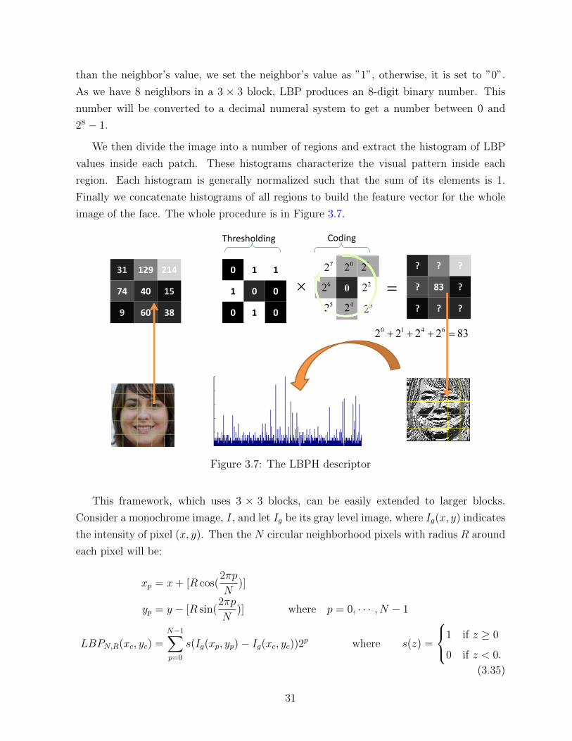
than the neighbor’s value, we set the neighbor’s value as ”1”, otherwise, it is set to ”0”.
As we have 8 neighbors in a 3 × 3 block, LBP produces an 8-digit binary number. This
number will be converted to a decimal numeral system to get a number between 0 and
28 − 1.
We then divide the image into a number of regions and extract the histogram of LBP
values inside each patch. These histograms characterize the visual pattern inside each
region. Each histogram is generally normalized such that the sum of its elements is 1.
Finally we concatenate histograms of all regions to build the feature vector for the whole
image of the face. The whole procedure is in Figure 3.7.
31 129 214
74 40 15
9 60 38
0 1 1
1 0 0
0 1 0
? ? ?
? 83 ?
? ? ?
0 ×
02
12
22
32
42
52
62
72
0 1 4 62 2 2 2 83+ + + =
Thresholding Coding
=
Figure 3.7: The LBPH descriptor
This framework, which uses 3 × 3 blocks, can be easily extended to larger blocks.
Consider a monochrome image, I, and let Ig be its gray level image, where Ig(x, y) indicates
the intensity of pixel (x, y). Then the N circular neighborhood pixels with radius R around
each pixel will be:
xp = x+ [R cos(2πp
N)]
yp = y − [R sin(2πp
N)] where p = 0, · · · , N − 1
LBPN,R(xc, yc) =N−1∑p=0
s(Ig(xp, yp)− Ig(xc, yc))2p where s(z) =
1 if z ≥ 0
0 if z < 0.
(3.35)
31
In the formula shown above, we must also take into consideration the following facts:
• In computing the pixel values, sampling points that are not on the sampling grid,
bilinear interpolation can be employed.
• Since extracting LBPN,R from images’ borders is not possible, only the central part
of the image is being considered.
This extension of LBP is a generic formulation of the operator that allows us to use a
larger neighborhood.
Uniform Patterns
One of the important characteristics of a good descriptor is its invariance to the rotation
of the target image. To this end, the uniform pattern has been proposed later by Ojala et
al. [72] as an extension of the LBP method. They [72] defined a uniformity measurement
U (pattern) that computes the number of bitwise transitions from 0 to 1, or 1 to 0. This
measurement is expressed as follows:
U(LBPN,R(Ig(xc, yc))) = |s(Ig(xN−1, yN−1)− Ig(xc, yc))− s(Ig(x0, y0)− Ig(xc, yc))|
+N−1∑p=1
|s(Ig(xp, yp)− Ig(xc, yc))− s(Ig(xp−1, yp−1)− Ig(xc, yc))|
(3.36)
For example,
pattern = ”00000000” ⇒ U(”00000000”) = 0
pattern = ”00000111” ⇒ U(”00000111”) = 1
pattern = ”00011000” ⇒ U(”00011000”) = 2
pattern = ”10011011” ⇒ U(”10011011”) = 4
They then map the pattern (p) to its corresponding number if the number of transitions
is less than or equal to 2 (U(p) ≤ 2) and the rest of the patterns are mapped to a unique
number. They applied this extension to the circular pattern extracted from LBP and
referred to it as the uniform local binary pattern (uLBP):
LBP riu2N,R =
∑N−1
p=0 s(Ig(xp, yp)− Ig(xc, yc)) if U(LBPN,R) ≤ 2
N(N − 1) + 3 otherwise(3.37)
32

The superscript riu2 shows the rotation invariant uniform patterns of the U function with,
at most, 2 bitwise transitions having been applied. This way of mapping for patterns can
be interpreted as encoding different local structures, such as spots, flat areas, edges, edge
ends, and curves, as shown in Figure 3.8:
Spot point Spot or flat point Endpoint of a line
Corner point Edge Non-uniform pattern
Figure 3.8: Examples of different texture structures detected by the LBP method (blackcircles represent of ones’ ”1”, and white circles correspond to zeros ”0”)
To this end, it has been observed that uniform LBP (uLBP) patterns have better
performances in recognition tasks when compared to LBP.
3.3.2 Scale-Invariant Feature Transform (SIFT)
The Scale Invariant Feature Transform (SIFT) descriptor proposed by Lowe [63] is a
powerful description method for characterizing image regions, which has been widely used
for various computer vision applications. SIFT produces a 128-dimensional representation
for each image region by employing a local gradient operator around the region’s center
point (which is called a keypoint). This representation is built by using a 3D (2 locations
and 1 orientation) histogram of gradient locations and orientations. In this process, each
patch surrounding a keypoint is scaled at different ratios, and then the orientation his-
togram over 4 × 4 regions is computed. The orientation of each region is computed from
a histogram of a gradient magnitude in eight directions. These orientation histograms
33

from 16 regions are concatenated and result in a 128 element feature descriptors. The
quantization of gradient locations and orientations makes SIFT descriptors robust to small
geometric distortions and certain illumination variations.
3.3.3 Binary Robust Independent Elementary Features (BRIEF)
The Binary Robust Independent Elementary Features (BRIEF), proposed by Calonder
et al. [14], is a binary descriptor that is fast and simple to compute. This approach is
similar to the method of LBP in terms of evaluating differences between intensity pixels.
The BRIEF method first smooths the image patches to reduce noise. Then, the differences
between the pixels’ intensity is employed to construct the descriptor. For this purpose,
Calonder et al. [14] defined a test τ between pixel I(x1, y1) and pixel I(x2, y2) by:
τ(I(x1, y1), I(x2, y2)) =
{1 if I(x1, y2) < I(x2, y2)
0 o.w(3.38)
The BRIEF descriptor for a patch is constructed in a k-length bitstring by performing a
test on a set of pixels within it. In order to generate this descriptor for a patch P , the
following score is computed for k = 128, 256, or 512:
dP =k∑i=1
2i−1τ(I(xi, yi)) (3.39)
In order to find an appropriate set of pixels, there are many ways to select them from a
patch size N × N . For this purpose, Calonder et al. [14] conducted an experiment over
the following five sampling geometries:
1 Selection has been done by using an i.i.d. Uniform(−N2, N
2) distribution, which means
that pixels are chosen by equivalent distribution from all pixels over the region.
2 Pixels have been sampled by an i.i.d. Gaussian(0, N2
25) distribution, which means
that they are employed by an isotropic Gaussian distribution with experimentally
adjusted variance equivalent to N2
25.
3 Pixels have been sampled by two zero mean i.i.d. Gaussian distributions, one with
variance N2
25centered on origin and another one with variance N2
100centered on the
selected pixel. These variances have been tuned by experiments to capture more local
information from a patch.
34

4 Pixels were chosen by random selection over a coarse polar grid.
5 K possible points over diagonals of coarse polar grid centered by I(0, 0).
Making use of their extensive recognition setup, Calonder et al. [14] reported that second
selection (i.i.d. Gaussian (0, N2
25)) leads to the best result in terms of recognition rate (i.e.
the rate of correct decisions to the number of overall decisions, which can be interpreted as
the Rank 1 identification rate). Furthermore, they claimed that the BRIEF descriptor is
robust against image blurs and illumination changes while still being sensitive to rotation
and scale changes.
3.3.4 Fast Retina Keypoint (FREAK)
The bio-inspired FREAK descriptor proposed by Alahi et al. [5] employed a retinal
sampling circular grid. The FREAK method employs 43 sampling patterns based on retinal
receptive fields that are shown in Figure 3.9.
! "!! #!! $!! %!! &!! '!!
!
"!!
#!!
$!!
%!!
&!!
'!!
Figure 3.9: 43 sampling patterns used in FREAK method
These 43 receptive fields are sampled by decreasing factors as the distance from the
patch’s center yields to a thousand potential pairs to extract a binary descriptor. Each
pair is smoothed with Gaussian functions, and then binary descriptors are generated by
setting a threshold and considering the sign of differences between pairs. For a pair, Pa,
this descriptor is defined by
D(Pa) =k∑i=1
2iT (Pa) (3.40)
35

where
T (Pa)
{1 if I(P r1a) > I(P r2a)
0 o.w(3.41)
As it would be preferable to select pairs with a high discriminant power and ignore
highly correlated ones, FREAK examined all possible choices for about 50,000 detected
keypoints in a set of images. It then sorts them based on their discrimination power.
This method selected the 512 most discriminative pairs. It group these 512 pairs into
four clusters - each having 128 pairs - which has the benefit of not only keeping the
symmetric scheme, but also of capturing the coarse-to-fine structure.
Another factor that should be considered is the fact that long-distance receptive fields
are used to capture orientation, and short-distance receptive fields are used to capture more
details from the patch. Consequently, the first resulting cluster is initially used to estimate
the position of the object of interest, and the short distance cluster is then used to validate
our estimation. This scheme approximates the human visual system by considering the fact
that humans look at a scene with discontinuous eye movements. This searching strategy is
called a ”Saccadic” search. The Saccadic search scheme in feature-matching applications
can dramatically reduce the processing time by discarding nontarget features as quickly as
possible by comparing only 16 bytes in the first cluster.
3.4 Block-based Bag of Words (BBoW)
The Bag-of-Words (BoW) method is a powerful technique in object recognition [82] that
represents an object by creating a histogram over extracted elements from sample images
from different categories. This method maps extracted features from a large domain to
a smaller one that is created by clustering meaningful elements extracted from similar
images. Z. Li et al. [59] applied this approach to face recognition by employing dense
SIFT features extracted from different patches through the image.
Since face objects all share the same basic structure and elements, each face can be
represented by building a histogram over a collection of candidates. This collection, called
codebooks, contains different candidates corresponding to different local regions, which are
called codewords. The main focal point of this approach is then creating rich codebooks
and representing each face in the form of occurrence frequency distribution of codewords
in the constructed codebooks.
When constructing codebooks, the first step is to divide face images into regions denoted
36

by patches. Then, features within each patch are extracted for all images. Those belonging
to certain specific areas are gathered and fed into the clustering process in order to be
partitioned into K clusters. By choosing a set of meaningful and appropriate features,
recognition become more robust against the noise and other possible intrinsic variations.
Once the codebook is created, the algorithm characterizes each region by mapping all
extracted feature vectors to the closest codewords for that region. In other words, each
region is described based on the occurrence statistics of the set of codewords. Finding the
closest codeword for each feature vector is based on a distance metric that depends on
the type of features. Euclidean distance, Hamming distance, Histogram Intersection, and
cosine similarity are among the most useful distance metric systems. The thus obtained
histograms are concatenated to represent the face to be used in the training and testing
stages. The whole procedure of our block-based bag of words (BBoW) method to extract
facial features for face recognition is shown in Figure 3.10.
Partition face
into 7×7 blocks
LBP feature
Extraction
Form 7x7
codebooks
Convert images
to 5x5 bags
of codewords
Represent images
as concatenated
histograms
Classification Matching session
Find the
best match
Training Testing
Figure 3.10: Framework of Block-Based bag of Words(BBoW)
37

As mentioned above, one of the main stages of BoW is to build an appropriate code-
books. For this purpose, different unsupervised methods can be employed, such as K -means
and random selections. In the subsequent sections, we briefly describe these two methods.
K -means Clustering
K-means clustering proposed by Stuart Lloyd [62], is a popular technique in data clus-
tering. This method finds certain points that correspond to the center of clusters by using
the fact that any point in a cluster is closer to its corresponding center than to the other
clusters’ centers.
Assuming there are K clusters with centers µ1, · · · , µK belonging to Rd space, K -
means clustering aims to minimize overall distances between all data and the corresponding
cluster’s centers:
L =K∑i=1
∑i:xi assigned to µj
||xi − µj||2 =K∑i=1
∑i:xi assigned to µj
αi,j||xi − µj||2 (3.42)
where
α(i, j) =
1 if xi assigned toj
0 o.w(3.43)
K -means tries to minimize L(3.42) with respect to all the αi,j and µj, by applying the
following iterations:
• Choosing an optimal set of αs for the fixed values of µs
• Choosing an optimal set of µs for the fixed values of αs
This greedy algorithm repeats these two iterations until convergence is achieved.
Random Selections
Random cluster selection is another popular technique in codebook construction. This
method, which requires fewer parameters to be tuned for constructing clusters, is popular
because of its simplicity and its ease of implementation. It simply consists in choosing a
random number of features from a large set of data. Studies have even shown [48] that
selecting clusters by K -means does not beget better results than random selection does.
In fact, by gathering a large number of features from each local region, K number of
38

features are randomly selected within features regarding each cluster label and will be
evenly distributed in the codebooks.
3.5 Matching face images for classification
Previous sections described how to extract features from a face image. These extracted
features are used in the next stage to find the nearest face in a dataset. This procedure can
be done by using Brute-force Matching, Support Vector Machine (SVM), Artificial Neural
Network (ANN), or a Bayesian classifier. As Brute-force Matching is quite simple and easy
to implement, we go over this method and apply it to find the nearest face in a trained
dataset. The SVM classifier is explained in chapter 4.
3.5.1 Brute-force Matching
Brute-force Matching is a popular and simple technique that is applicable to a wide
variety of problems, including face identification challenges. In this approach, we find the
best match for a face object among the stored faces. Once a face is captured, features
regarding the face are extracted and the closest pre-extracted feature vector is found.
Finding the closest face is dependent on the type of extracted features and how the distance
between them is computed. To identify a face among a set of faces, there are two factors to
analyze: an appropriate distance metric and the setting of a threshold for the identification
of unknown individuals. The next section presents different forms of measurement for the
histogram and Hamming distances, while identification of unknown faces is discussed in
the results section.
3.5.2 Compare Histograms
Of particular interest to us is the case of histogram descriptors. The Local binary
pattern histogram and the Bag-of-Words methods collect occurrence statistics of each
image by using a histogram representation. To compare these types of descriptors, the
Histogram Intersection, Chi-Square, and Correlation method can be employed.
The Histogram Intersection is a robust technique that is not affected by rotation and
small changes in distance. This distance is defined as follows:
39

d(H1, H2) =n∑i=1
min(h(i)1 , h
(i)2 )) (3.44)
Another measurement for histogram comparison is the Chi-Square method. Inspired
by the χ2 test-statistic [83], this method has been employed in several texture and object
categories’ classification algorithms (e.g. [23], [99], [93], and [8]). In the most cases, the
differences between large bins in histogram is less important than the difference between
small bins. So Chi-Square distance is defined by the fact that differences between the large
bins’ value being equivalent to the differences between the small bins’ value. This can be
accomplished by taking the norm of the bins into account. The two following equations
are popular measurements to compute this distance:
d(H1, H2) =n∑i=1
(h(i)1 − h
(i)2 )2
h(i)1
d(H1, H2) =n∑i=1
(h(i)1 − h
(i)2 )2
h(i)1 + h
(i)2
(3.45)
The Correlation Method considers each histogram as a 1-D signal. It then computes the
correlation with the following formula:
d(H1, H2) =
∑ni=1(h
(i)1 − h1)(h
(i)2 − h2)√
[∑n
i=1(h(i)1 − h1)2][
∑ni=1(h
(i)2 − h2)2]
(3.46)
In the Histogram Intersection distance and the Correlation distance, a high score value
indicates that the two histograms present a measurably better match than two histograms
with a low score value. Conversely, the lowest value in the Chi-Square method indicates
that the two histograms are a better match.
These bin-to-bin distances are generally sensitive to quantization effects, and the dif-
ferences between their accuracy is not very significant. Therefore, because of its ease of
implementation, Histogram Intersection is selected here.
3.5.3 Hamming Distances
Once features have been extracted, we can compare them by different distance mea-
surements. The BRIEF and FREAK methods are associated with constructing binary
descriptors for images. In this case, for two k-length binary descriptors D(I1) ∈ {0, 1}k
40

and D(I2) ∈ {0, 1}k that represent two points in k dimensional Hamming space, the Ham-
ming distance is defined as
Ham(D(I1), D(I2)) =k∑i=1
Di(I1)⊗Di(I2) (3.47)
where ⊗ is the single instruction bitwise XOR operation.
3.6 Experimental Results
This section provides the result of the described methods on two publicly available
databases: the FERET and LFW database. All codes are implemented in C++ using
the OpenCV 2.4.2 library, which is an open source library specialized for computer vision
applications.
The rest of this section is organized as follows: Section 3.6.1 describes the two publicly
available databases which have been used to evaluate our methods. In section 3.6.2 we
compare two global representation approaches, PCA and LDA, with the LBPH feature-
based technique. Then, in sub-section 3.6.3 we employ edge detection techniques to remove
the artifacts induced by noise and appearance changes. In contrast to the previous sub-
section, we use the results of the edge detection techniques as an input of PCA, LDA,
and LBPH, and we show that a significant improvement can be obtained by using these
techniques. In section 3.6.4, we evaluate the SIFT, BRIEF and FREAK descriptors on
the FERET and LFW database. Thereafter, in section 3.6.5 we analyze Bag-of-Words
method on the SIFT and LBPH descriptors. Finally, in section 3.6.6, we propose a model
to detect unknown individuals. Additionally, extensive experimentation has been carried
out to determine the optimal value for parameters of our face recognition framework.
3.6.1 Dataset
The performance of the different descriptors explained above has been evaluated using
standard benchmark databases for face recognition: the Facial Recognition Technology
(FERET) database and the Labeled Faces in the Wild (LFW) database.
41

The Facial Recognition Technology (FERET) Dataset
The FERET Database [75] of face images collected between August 1993 and July 1996,
contains 1564 sets of images for a total of 14,126 images. These images were captured
at a variety of illumination levels, face positions and includes people with various facial
expressions, ages, degrees of occlusion, and facial hair. The image data has been captured
at a resolution of 180× 200. Some other information, such as age, ethnicity, and gender is
also included in the database ground truth files.
A set of different categories of images in the database is shown in Figure 3.11. Among
these categories, the five frontal views (Fa, Fb, Fc, Dup I, and Dup II) are the most
popular.
• Fa probes: images are taken of neutral facial expressions, all with the same lighting
(1196 images)
• Fb probes: images are captured with an alternative frontal expression seconds after
the Fa (1195 images)
• Fc probes: images are taken under different levels of illumination (194 images)
• Dup I probes: images are taken anytime between one minute and 1031 days after the
corresponding Fa (722 images)
• Dup 2 probes: images are taken at least 18 months after their corresponding Fa (234
images)
All images in the database are cropped and normalized by employing an affine transform
to the size of 100 × 100 using the coordinates of the faces’ eyes and mouths as given by
ground truth.
Figure 3.11: Sample faces in FERET database
42

Labeled Faces in the Wild (LFW) Dataset
The LFW database [43] is a rich database containing over 13,000 photographs of faces
in unconstrained conditions which were collected from the Web. The LFW images are cap-
tured from faces with a variety of poses, illuminations, backgrounds, expressions, clothing,
hairstyles, cosmetics, and so on. These images belong to people of different ages, gen-
ders, and ethnicities and are good examples of the real world images with which most face
recognition applications strive to work. As such, training a system to employ this type of
database, ensures that the proposed system can be generalized to real-world applications.
Later, a commercial system [42] was used to align the images in the LFW database so
that the positions of the faces’ eyes and mouths would be the same for all face images.
Of the 5,749 individuals in this database, 4,069 people have only one image and the
others have two or more images. In order to build a dataset suitable for face recognition
benchmarking, we collected a set of face images from 20 individuals having 10 images per
person.
Figure 3.12: Collected LFW database
It must be noted that the LFW database has more face images includes people of West-
ern ethnicities than of other ethnic groups. Also, much like the FERET database, LFW
43

images were taken in a short period of time. Therefore, a good verification performance
on LFW does not necessary guarantee effectiveness in a real environment.
In this section we go through the described methods and test them on two LFW and
FERET frameworks for face recognition.
3.6.2 Analysis of PCA, LDA, and LBPH
In this section, the performance of PCA, LDA and LBPH were evaluated for the purpose
of face identification on the FERET and LFW databases. Two FERET image sets (Fa
and Fb) have been used in our face recognition test. In this experiment the 1,196 images
in the Fa probe were used for training, and the system was tested on the 1,195 images of
the Fb probe. All images in the training or testing sets were scaled to 100× 100.
In face identification, one of the most important parameters is the size of the available
database. Since increasing the number of training samples would change the results, a
good testing would include testing and training sets of different sizes. For this purpose, we
tested random sets of 100, 300, and 800 in five runs on the FERET database. The results
for the entire database are reported in the last column of Table 3.1.
Table 3.1: The recognition rate of PCA, LDA, and LBPH with different numbers of trainingon the Fb probe set of the FERET database. First row indicates the number of imagesused for training and, under parantheses, the number of test images
Methods 100(100) 300(300) 800(800) 1196(1195)
PCA 75.62 69.67 64.43 71.11
LDA 73.15 69.33 62.74 68.43
LBPH 90.8 88.12 82.68 78.39
As it can be seen, LBPH performs better than PCA and LDA. In the next step, we
test these methods to evaluate their robustness against the other parameters such as illu-
mination and the aging factor. As mentioned in the previous section, the FERET dataset
provided the Fc that contains illumination changes, and Dup I and Dup II that includes
aging over time. By testing these probes, it is evident that the tested methods appear to
be sensible to these changes, as shown in Table 3.2.
44

Table 3.2: The recognition rate of PCA, LDA, and LBPH on the FERET database probesets trained using Fa set.
Methods Fa(Fb) Fa(Fc) Fa(Dup I) Fa(Dup II)
PCA 71.11 11.86 23.96 8.99
LDA 68.43 15.76 22.02 10.27
LBPH 78.39 23.71 28.39 11.98
We also tested these methods on the LFW database ([43]). This evaluation is repeated
over nine iterations, where, at iteration i, the first i images are used for training and the
last (10− i) images are used for testing. As seen in Table 3.3, LBPH seems to be superior
when the number of training images increases.
Table 3.3: The recognition rate of PCA, LDA, and LBPH on the LFW database
Methods 10(90) 20(80) 30(70) 40(60) 50(50) 60(40) 70(30) 80(20) 90(10) average
PCA 21.11 19.38 27.14 28.33 30 33.75 35 37.5 35 26.78
LDA 16.67 29.38 36.43 47.5 58 55 55 57.5 55 39.34
LBPH 22.78 35.63 41.43 44.17 51 52.5 50 52.5 50 40.33
3.6.3 Analysis of Edge Detection Operators
In this section, we evaluate various types of edge detection operators on our data. The
objective of using edge detectors is to limit the effect of some parameter variations such as
illumination and age from the face’s main structure. We first apply different edge detectors
such as Sobel, Canny, and Laplacian operators on the image. Then, the resulting image is
fed into the PCA, LDA, and LBPH methods to extract their face descriptors.
The results of these operators on Fc probes of the FERET database are reported in
Table 3.4:
45

Table 3.4: The recognition rate of PCA, LDA, and LBPH methods combined with differentedge operators on the Fc probe of the FERET database
Methods Sobel Laplacian Canny raw image
PCA 65.46 30.31 53.09 11.86
LDA 64.95 35.91 59.79 15.76
LBPH 60.31 43.21 31.96 23.71
The parameters responding of these edge operators, such as kernel size, and sigma size,
have been tuned to get the best result possible. It is evident that employing edge detector
operators improves the algorithms’ robustness against the illumination changes. The best
combination corresponds to the Sobel and PCA methods.
We also tested the above-mentioned methods on three other categories in the FERET
dataset: Fb, Dup I, and Dup II. The Sobel edge detector once again outperformed the
other edge detection methods. The results are provided in Table 3.5.
Table 3.5: The recognition rate of the PCA, LDA, and LBPH combined with the Sobeledge operators on the FERET database probe sets
Methods Fa(Fb) Fa(Dup I) Fa(Dup II)
PCA+Sobel 48.41 26.48 15.56
LDA+Sobel 42.38 22.33 13.42
LBPH+Sobel 80.49 31.16 28.39
In the next experiment, we employed this method to test face recognition performance
in an uncontrolled environment. For this purpose, we tested this method on the LFW
dataset:
Table 3.6: The recognition rate of PCA, LDA, and LBPH combined with Sobel edgeoperators on the LFW database
Methods 10(90) 20(80) 30(70) 40(60) 50(50) 60(40) 70(30) 80(20) 90(10) average
Sobel+PCA 19.44 28.75 26.43 28.33 29 31.25 33.33 30 40 27.33
Sobel+LDA 20 16.25 18.57 30 31 31.25 40 32.5 45 25.11
Sobel+LBPH 27.78 38.75 45.71 45 51 55.25 48.33 52.5 50 42.8
46

It can be seen in Table 3.6 that extracting a histogram of local binary patterns sig-
nificantly outperforms the PCA and LDA methods. Adding Sobel to LBPH and PCA
methods improved their discriminating power, but it is still far from the acceptable per-
formance necessary for real-world applications.
3.6.4 Analysis of SIFT, BRIEF, and FREAK methods
In this section, we report results of applying the SIFT, BRIEF, and FREAK methods on
our two benchmark datasets. As we previously explained, SIFT produces a 128-dimensional
representation for each image region using a 3D (2 locations and 1 orientation) histogram
of gradient locations and orientations. The use of the BRIEF and FREAK methods as
texture-encoding descriptors based on local binary patterns was also tested. It should be
mentioned that the distances between BRIEF and FREAK descriptors are computed by
Hamming distance. The results of these methods on four probes of Fb, Fc, Dup I, and
Dup II are given in Table 3.7.
Table 3.7: The recognition rate of the SIFT, BRIEF, and FREAK methods on the FERETdatabase probe sets
Methods Fa(Fb) Fa(Fc) Fa(Dup I) Fa(Dup II)
SIFT 86.18 77.84 46.24 22.22
BRIEF 78.57 35.54 36.43 16.24
FREAK 76.72 48.45 36.70 24.36
As expected, the SIFT method shows better result on the Fc probes, which shows the
robustness of this method against illumination variations.
Thus, in real world situations where all possible variations can be observed, a recogni-
tion task based on methods which are sensitive to appearance variations have a low level
of accuracy. To demonstrate this, the results of empirical investigation on the LFW have
been shown in Table 3.8.
47

Table 3.8: The recognition rate of the SIFT, BRIEF, and FREAK methods on the LFWdatabase
Methods 10(90) 20(80) 30(70) 40(60) 50(50) 60(40) 70(30) 80(20) 90(10) average
SIFT 33.89 46.25 57.86 60 63 68.75 63.33 65 60 53.56
BRIEF 25.56 32.5 38.57 41.67 46 51.25 53.33 55 55 39.33
FREAK 27.78 35.63 45.71 46.67 48 53.75 55 57.5 60 42.89
The above results show how popular methods for feature extraction offer results for
face recognition that are far from acceptable.
From the results indicated above, it is evident that recognizing a face simply employing
powerful descriptors cannot lead us to an accurate system. A good approach to tackling
this problem is to apply methods that try to describe the captured using global structures.
In the subsequent section, we test the BoW method on the LFW dataset to show how much
our results can be improved by adjusting and finding appropriate parameters to reach the
best possible results.
3.6.5 Analysis of the BoW approach
In this section we experiment the Bag-of-Words approach on the LFW and FERET
datasets. Here, the Bag-of-Words method is constructed from features extracted by LBP
and SIFT descriptors and then its corresponding parameters are set to improve the recog-
nition accuracy.
As previously mentioned, choosing the closest word in codewords depends on the type of
descriptors. To compare histograms of LBP features, we use Hamming distance as a simple
and quick distance metric, and for SIFT descriptors we employ Euclidean measurements.
Making use of the Bag-of-Words method requires to tune the different parameters. In
the following example, LBP and SIFT were extracted in a window size of 8 by 8 around
pixels with a distance of 4 along the x-axis and 3 along the y-axis. One feature vector is
calculated on the center of each grid. Finding the appropriate size of gridding schemes is
another parameter which should be carefully set. We later test different visual words on
each block with different grid sizes. In Table 3.9, the results of applying BoW methods
over LBP, uLBP and SIFT features in different gridding schemes with 20 number of words
for each region is provided:
48

Table 3.9: The recognition rate of the BoW method on features extracted by LBP, uLBP,and SIFT methods on the LFW database
Methods Gridding Scheme 10(90) 20(80) 30(70) 40(60) 50(50) 60(40) 70(30) 80(20) 90(10) average
BoW-LBP 4× 4 32.78 50.63 58.57 60.83 60 62.5 63.33 62.5 55 53.22
BoW-LBP 7× 7 40.18 48.96 62.62 64.45 71.3 75 73.3 73.3 65 59.25
BoW-uLBP 7× 7 40.56 48.75 62.39 63.61 69.7 65.42 71.67 69.17 58.33 57.67
BoW-uLBP 8× 8 35 40 53.57 59.17 65 63.75 63.33 65 65 51.78
BoW-SIFT 7× 7 32.7 43.13 52.86 54.17 60 67.5 73.3 67.5 65 51.65
As seen in Table 3.9, BoW on LBP feaature with gridding size 7 × 7 performs better
than others. But processing the 256-bin histogram is so expensive in comparison with
59-bin histogram in terms of memory and speed.
The results of BoW method over LBP features on four probes of Fb, Fc, Dup I, and
Dup II with 20 number of words have been provided in the following table:
Table 3.10: The recognition rate of BoW method over LBP features on the FERETdatabase probe sets
Methods Fa(Fb) Fa(Fc) Fa(Dup I) Fa(Dup II)
BoW-uLBP 93.05 84.43 46.88 23.94
As shown, it is obvious that the tuning of parameters to optimize a subset of the results
is a necessary step in the BoW method. If this step is omitted, results may vary by a large
number.
One of the other main configuration in this procedure is face alignment. Since each
element should be represented by the correct words, they should be located in the right
positions. To clarify this matter, we have done an experiment based on face alignment using
different potential locations of eyes. By changing the eyes’s locations, unrelated words are
employed to represent the eyes recognition accuracy will be reduced. The results of this
experiment based on gridding scheme 7× 7, 20 number of words, and (xstep, ystep) = (4, 4)
have been provided in the following table. The second row corresponds to the alignment
of faces where the eyes’ locations in first row changed only by 5 px; in the third row,
they changed by 10 px. These changes are applied in the Y-direction, and the codewords
corresponding to each grid have not been changed:
49
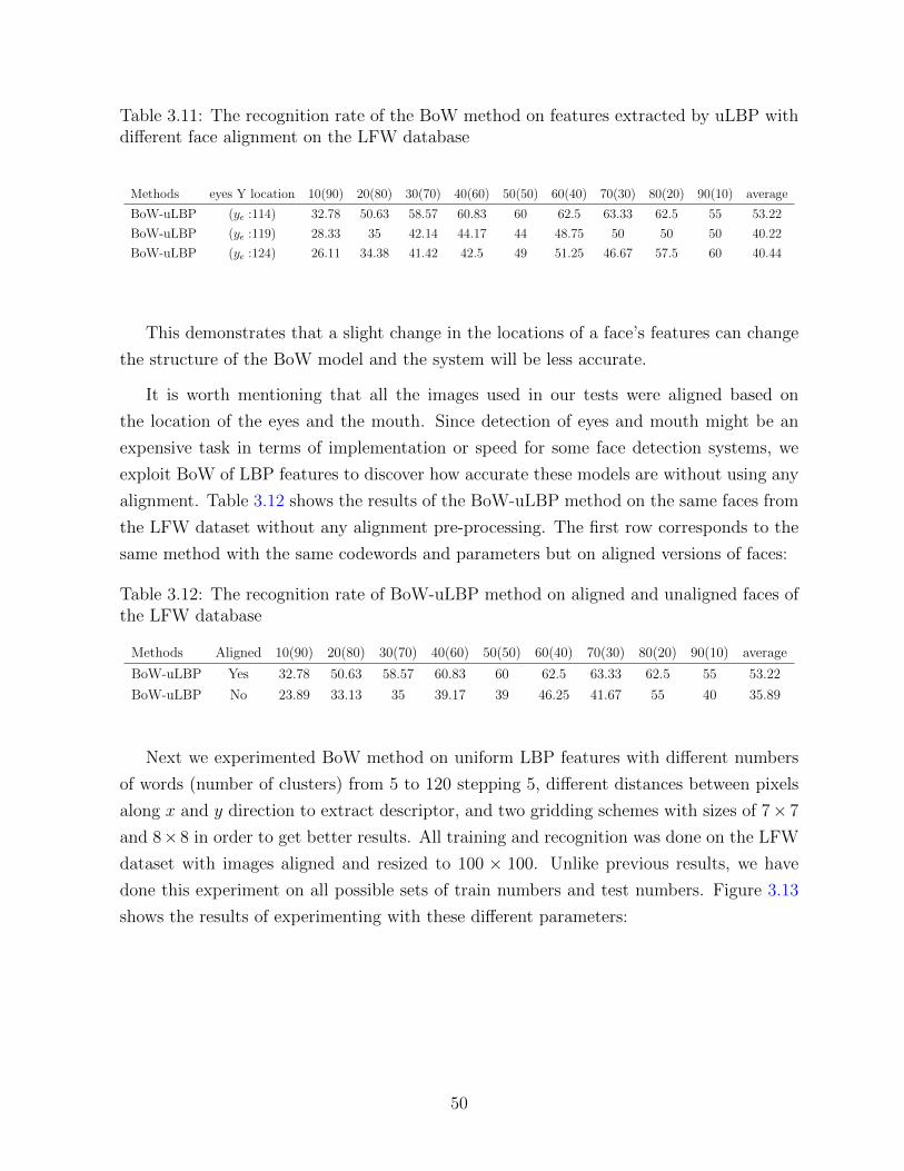
Table 3.11: The recognition rate of the BoW method on features extracted by uLBP withdifferent face alignment on the LFW database
Methods eyes Y location 10(90) 20(80) 30(70) 40(60) 50(50) 60(40) 70(30) 80(20) 90(10) average
BoW-uLBP (ye :114) 32.78 50.63 58.57 60.83 60 62.5 63.33 62.5 55 53.22
BoW-uLBP (ye :119) 28.33 35 42.14 44.17 44 48.75 50 50 50 40.22
BoW-uLBP (ye :124) 26.11 34.38 41.42 42.5 49 51.25 46.67 57.5 60 40.44
This demonstrates that a slight change in the locations of a face’s features can change
the structure of the BoW model and the system will be less accurate.
It is worth mentioning that all the images used in our tests were aligned based on
the location of the eyes and the mouth. Since detection of eyes and mouth might be an
expensive task in terms of implementation or speed for some face detection systems, we
exploit BoW of LBP features to discover how accurate these models are without using any
alignment. Table 3.12 shows the results of the BoW-uLBP method on the same faces from
the LFW dataset without any alignment pre-processing. The first row corresponds to the
same method with the same codewords and parameters but on aligned versions of faces:
Table 3.12: The recognition rate of BoW-uLBP method on aligned and unaligned faces ofthe LFW database
Methods Aligned 10(90) 20(80) 30(70) 40(60) 50(50) 60(40) 70(30) 80(20) 90(10) average
BoW-uLBP Yes 32.78 50.63 58.57 60.83 60 62.5 63.33 62.5 55 53.22
BoW-uLBP No 23.89 33.13 35 39.17 39 46.25 41.67 55 40 35.89
Next we experimented BoW method on uniform LBP features with different numbers
of words (number of clusters) from 5 to 120 stepping 5, different distances between pixels
along x and y direction to extract descriptor, and two gridding schemes with sizes of 7× 7
and 8×8 in order to get better results. All training and recognition was done on the LFW
dataset with images aligned and resized to 100 × 100. Unlike previous results, we have
done this experiment on all possible sets of train numbers and test numbers. Figure 3.13
shows the results of experimenting with these different parameters:
50
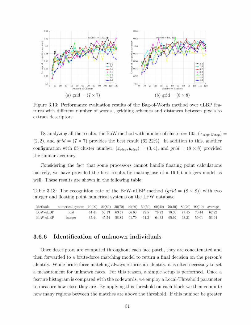
0 10 20 30 40 50 60 70 80 90 100 110 1200.5
0.52
0.54
0.56
0.58
0.6
0.62
0.64
acc(105) = 0.62222
Number of Clusters
Ave
rage
ofre
cogn
itio
nac
cura
cy
2-22-33-23-33-44-34-4
(a) grid = (7× 7)
0 10 20 30 40 50 60 70 80 90 100 110 1200.5
0.52
0.54
0.56
0.58
0.6
0.62
0.64
acc(65) = 0.62222
Number of Clusters
Ave
rage
ofre
cogn
itio
nac
cura
cy
2-22-33-23-33-44-34-4
(b) grid = (8× 8)
Figure 3.13: Performance evaluation results of the Bag-of-Words method over uLBP fea-tures with different number of words , gridding schemes and distances between pixels toextract descriptors
By analyzing all the results, the BoW method with number of clusters= 105, (xstep, ystep) =
(2, 2), and grid = (7 × 7) provides the best result (62.22%). In addition to this, another
configuration with 65 cluster number, (xstep, ystep) = (3, 4), and grid = (8 × 8) provided
the similar accuracy.
Considering the fact that some processors cannot handle floating point calculations
natively, we have provided the best results by making use of a 16-bit integers model as
well. These results are shown in the following table:
Table 3.13: The recognition rate of the BoW-uLBP method (grid = (8 × 8)) with twointeger and floating point numerical systems on the LFW database
Methods numerical system 10(90) 20(80) 30(70) 40(60) 50(50) 60(40) 70(30) 80(20) 90(10) average
BoW-uLBP float 44.44 53.13 63.57 66.68 72.5 76.73 78.33 77.45 70.44 62.22
BoW-uLBP integer 35.44 45.54 58.82 61.79 64.2 64.32 65.92 63.21 59.01 53.94
3.6.6 Identification of unknown individuals
Once descriptors are computed throughout each face patch, they are concatenated and
then forwarded to a brute-force matching model to return a final decision on the person’s
identity. While brute-force matching always returns an identity, it is often necessary to set
a measurement for unknown faces. For this reason, a simple setup is performed. Once a
feature histogram is compared with the codewords, we employ a Local-Threshold parameter
to measure how close they are. By applying this threshold on each block we then compute
how many regions between the matches are above the threshold. If this number be greater
51

than x% of image’s regions we keep the identity as a right person, if not we set it as a new
person. This number of regions has been carefully set for the LFW dataset.
In this experiment we added the 50 different faces from LFW dataset as unknown indi-
viduals to test set. The results are the average of right recognition based on the recognizing
true identity and unknown ones. We experimented with different values of Local-Threshold
parameters (5, 10, 11 , · · · , 15, 20), and regions number in the best configuration in gridding
schemes of 7 × 7 in order to get better results. All training and recognition was done on
the LFW dataset with images aligned and resized to 100× 100.
4 6 8 10 12 14 16 18 200.1
0.2
0.3
0.4
0.5
0.6acc(12) = 0.585
Local-Threshold
Ave
rage
ofre
cogn
itio
nac
cura
cy
20%30%40%50%60%
Figure 3.14: Performance evaluation results of the Bag-of-Words method with 50 unknownfaces with different threshold and number of regions
By analyzing all the results, the BoW method with Local-Threshold= 12, number of
clusters= 115, (xstep, ystep) = (2, 2), matching 40% of regions in grid = (7×7) provides the
best result (57.24%).
3.7 Conclusion
In this chapter, different approaches for describing face images were described and
implemented. Their performances were empirically tested on two databases: FERET and
a restricted version of LFW. Among the described methods, we came up with the BoW
framework based on uniform LBP features. For this purpose, we conducted an extensive
parameter tuning experiment. The corresponding optimal parameters were provided in the
results section.
Overall, we found that employing the Bag-of-Words method for face recognition leads
to a significantly better performance when compared to the other tested methods when
52

used in realistic situations. Furthermore, as the local binary pattern method can be used
in face detection algorithms, designing a face recognition system based on this type of
feature is beneficial in terms of processing operations and speed. Furthermore, we used
the “Local-Threshold” parameter in cases where the detected face is not in our database.
53
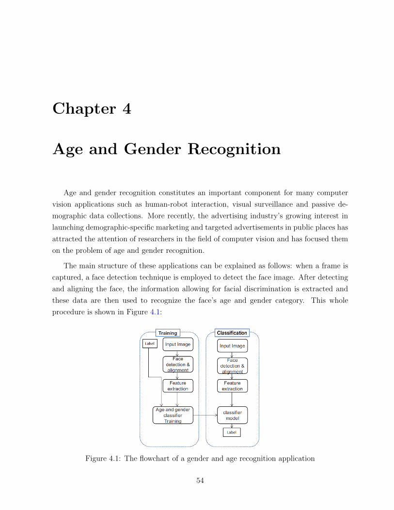
Chapter 4
Age and Gender Recognition
Age and gender recognition constitutes an important component for many computer
vision applications such as human-robot interaction, visual surveillance and passive de-
mographic data collections. More recently, the advertising industry’s growing interest in
launching demographic-specific marketing and targeted advertisements in public places has
attracted the attention of researchers in the field of computer vision and has focused them
on the problem of age and gender recognition.
The main structure of these applications can be explained as follows: when a frame is
captured, a face detection technique is employed to detect the face image. After detecting
and aligning the face, the information allowing for facial discrimination is extracted and
these data are then used to recognize the face’s age and gender category. This whole
procedure is shown in Figure 4.1:
Figure 4.1: The flowchart of a gender and age recognition application
54

As previously mentioned, a key component in any face processing system is facial
representation. While some methods choose to use raw pixels (e.g., [70], [38] and [78])
without any modification, the majority of the existing methods use local visual descriptors
to produce stronger and, often, more compact representations of face images. Examples of
visual information commonly used for age and/or gender recognition are features related
to texture information (e.g., used in [55],[53],[54], [85], [91] and [3]), shape information
(e.g., used in [88], [27] and [13]) and color information (e.g., used in [60] and [45]). These
methods employ local descriptors, which are often extracted from a dense regular grid,
over the entire image and then the face representation is built by concatenating these ex-
tracted descriptors into a single vector. A key issue in this framework is to determine the
optimal grid parameters (e.g., spacing, size, number of grids in multi-resolution/pyramid
approaches, etc.). The majority of methods that were mentioned in section 2.2 used fixed
settings and performed trial-and-error heuristics to determine the right grid parameters.
However, a better approach would be to use feature selection to allow the most informa-
tive image regions (or grid cells) those that can best separate face images that belong
to different demographic classes (with respect to age and gender) to contribute to the
facial representation. This approach further facilitates the integration of different types of
descriptors and allows for more compact representations by preventing redundant features
from contributing to the facial representation.
In this thesis, we suggest using feature selection to integrate different types of de-
scriptors (color-based, shape-based, texture-based, etc.) and compact representations by
preventing redundant features from contributing to the face representation. The approach
demonstrated in [88] also uses feature selection but in the context of gender recognition
only. They 1 used LBP, intensity histograms and gradient orientation features, while in
this thesis LBP, SIFT and color descriptions are employed. We performed both gender
recognition and age classification on two datasets: Gallagher’s and FERET.
The remainder of this chapter is organized as follows: in Section 4.1, we describe
the different steps of the proposed facial representation method. Section 4.2 explains
Ullman feature selection as a technique to select a set of the most discriminant features.
Section 4.3 describes the learning and classification modules and section 4.4 presents the
implementation details and experimental results.
1https://codeload.github.com/uricamic/flandmark/zip/master
55

4.1 Facial Representation
As previously mentioned, extracting the most useful facial information has been the
motivation behind most of the research in the field of face processing. Gender and age
classifications are among the most important applications of this field, which try to extract
information regarding the demographic category of the image of a face. The vast majority
of the existing solutions focus on a single visual descriptor which often encodes only a
certain characteristic of the image regions (e.g., shape, texture, color, etc.). Unlike these
methods, which normally only use a single type of descriptor based on a fixed setting
(in terms of grid parameters), in our proposed method, a face image is represented by a
collection of different types of local descriptors extracted from various regions across the
image. We do this because, though each type of visual descriptor only captures specific
information about an image region, they can all be used to complement the information
captured by another type of descriptor. For example, while the Local Binary Pattern (LBP)
descriptors encode spatial relations between neighboring pixels and are useful to describe
the texture of an image patch, a Scale Invariant Feature Transform (SIFT) builds local
histograms of gradient orientations and is the best when it comes to capturing the shape of
an image patch. Therefore, extracting both SIFT and LBP descriptors from their respective
locations in the face image (e.g., cheeks for LBP descriptors to distinguish between faces
with and without beards, and the nose and mouth for SIFT descriptors to distinguish
between different faces based on the shape characteristics of the facial features) allows
the produced face representations to take advantage of both sources of information. This
will, in turn, provide better distinctiveness between faces for classification and recognition
purposes.
To determine which type of visual descriptors are the most informative at specific
regions of the face image, we suggest using feature selection (where a feature is defined by
of type of descriptor and an image region) to choose the optimal set of features from a pool
of candidate features. In the next two sub-sections, we explain how the pool of candidate
features can be generated and how informative features can be selected.
4.1.1 Pool of Candidate Features
To generate the pool of candidate features, alignment techniques, which are based on
the affine transformation determined from three facial landmarks (left eye, right eye and
mouth center) must be used. For each aligned face image in the training set, an image
pyramid is built and then different types of visual descriptors are extracted from dense
56

regular grids (with different sizes and spacing of the pixels) over the image at each level
of the pyramid. This results in a large number of descriptors being extracted from various
regions of the face images. In this thesis, we consider three such types of features, each
encoding a certain characteristic (e.g. texture, shape and color) of an image region.
4.1.2 Texture Features
Among the variety of techniques that have been developed for extracting texture fea-
tures from a face image, the Local Binary Pattern Histogram(LBPH) and the Gabor
Wavelet technique number among the most successful ones. In this section, we will go
over these methods and briefly describe each of them.
The Local Binary Pattern Histogram
LBPH [72] as described in 3.4, is a powerful texture-encoding descriptor based on the
occurrence statistics of a set of local binary patterns. These uniform patterns help keep
it robust against the rotation and extract the more meaningful textures of the target
image. A uniform pattern is a Local Binary Pattern (LBP) with at most, two bitwise
transitions (or discontinuities) in the circular presentation of the pattern. When using
a 3 × 3 neighborhood, for example, only 58 of the 256 total patterns are uniform. In a
59-dimensional image representation (i.e., a histogram), there is one dimension for each
uniform pattern and one dimension for the entirety of the non-uniform patterns. The whole
procedure of applying LBPH has been explained in section 3.3.1
Gabor Texture Descriptors
The bio-inspired Gabor filter method, proposed by Gabor in 1946[33], is a texture
descriptor that is mainly inspired from the structure of the human retina. When observing
the cell layers in the retina, one can see that different types of cells exist. Hubel and
Wiesel[44] categorized the receptive fields of cells in the visual cortex into three categories:
simple cells, complex cells and hyper complex cells. Of these, a simple cell is defined as a cell
that responds primarily to oriented edges and gratings (bars of particular orientations).
The two-dimensional Gabor function models these types of cells based on their spatial
summation properties.
As this filter extracts the frequency and orientation characteristics of a region, it is
well suited for the texture analysis of images. In the spatial domain, a 2D-Gabor filter is
57

defined as a Gaussian kernel function modulated by a sinusoidal plane wave as follows:
G~k(~x) =||~k||σ2
.e−||~k||2.||~x||2
2σ2 .[ei~k.~x − e−
σ2
2
]~k = kse
iφ ks =π
2s+1
(4.1)
where ”s” corresponds to the scale of the Gaussian envelop, which takes on the values of
0, 1, · · · , 4 and ”φ” controls its orientation and takes on the values of 0, 1, · · · , 7. By using
5 scales and 8 orientations, a total of 40 Gabor filters are computed. Figure 4.2 represents
the section of the real part of the 40 Gabor filters.
Figure 4.2: Representation of the real part of 40 Gabor filters
Since computing Gabor coefficients for all pixels leaves a huge amount of information
requiring processing, statistical techniques such as PCA are commonly used to reduce the
amount of dimensions in which feature data is found.
58

4.1.3 Shape Features
Since human perception systems can provide a good approximation of age and gender
just by considering the shape of the face and its overall structure, descriptors which char-
acterize the shape information of image regions have received considerable attention. Of
a variety of descriptors commonly used for this purpose, we can mention different edge
operators and the Scale-Invariant Feature Transform (SIFT) as the most performant ones.
Note that SIFT can also be categorized as a textural descriptor. The high discriminative
power of SIFT descriptors acts as competition against different edge operators, which sim-
ply extract gradient orientation features and are not robust against the scale and rotation
variations. Thus, to recognize age and gender, we employ SIFT descriptors. The results
of this descriptor are found in section 4.4.
Scale-Invariant Feature Transform (SIFT)
As previously mentioned in section 3.3.2, SIFT [63] is a powerful description method
for characterizing image regions that has been widely used for various computer vision
applications. SIFT produces a 128 dimensional representation for each image region using
a 3D (2 locations and 1 orientation) histogram of gradient locations and orientations. The
contribution of each pixel to the location and orientation bins is weighted by its gradient
magnitude. The quantization of gradient locations and orientations makes SIFT descriptors
robust to small geometric distortions and certain illumination variations.
4.1.4 Color Features
Modeling color distribution can be very useful in characterizing an image region. For
this purpose, different types of color descriptors are used to describe image regions and
embed color information into an object recognition framework. In this section, two popular
techniques to fulfill this purpose - the color histogram and Color CENTRIST - are analyzed
and employed in the practice of age and gender recognition. A third color descriptor based
on the Local Binary Pattern framework(CLR-LBP) is also proposed and, through extensive
experiments, it is shown that our descriptor achieves results comparable with the two other
color descriptors.
59

Color Histogram
This type of descriptor models color distribution by constructing a histogram with 4
bins per color channel, in the RGB color space[45]. More specifically, the intensity values
in each color channel (i.e., red, green and blue) are mapped into 4 values (intensity values
between 0 and 63 are mapped to 0, and so on). Then, each of the 64 (43) bins stores
an integer that count the number of times the corresponding color triplet occurred. A
histogram is then computed using the corresponding quantized samples per pixel for each
region. Since each channel is mapped into 4 values, the histogram is specified by 64 bins.
The entire procedure that this descriptor undergoes is presented in the Figure 4.3.
!"#"$%&'()*%
+$,'-."$/%
!
"!#$!!!##!!!$$%!
!
01,'+&2,+&"'%
+,3#)%
!"#$%&#"'$ ()*"$%&#"'$
+,""&$%&#"'$
&'()*!#+,!
++$!
+#!
Figure 4.3: Color Histogram descriptor
Color CENTRIST
Chu et al. [20] developed a new descriptor to categorize image scenes: Color CEN-
TRIST. This descriptor, based on the CENsus TRansform hISTogram (CENTRIST)[97]
framework, employs both intensity gradients values and color variations among image
pixels. The goal of the CENTRIST framework is to compensate for two existing issues
prevalent in histogram-based descriptors: disappearing spatial information from the his-
tograms during the computation process and a lack of multilevel representation. To tackle
these problems. Chu et al. proposed a spatial pyramid scheme, which scales images to
different levels. In the k level, an image is divided into regions with a size of N2k× N
2k. Next,
they split the image’s width and height into 2k parts and all resultant regions plus the ones
centered at the common corners of four neighboring regions are extracted. By this scheme
for image level k we have 22k+1 − 2k+1 + 1 number of regions.
60

Level 0
Level 1
Level 2
Figure 4.4: Illustration of levels 2, 1, and 0 split of an image
The Color CENTRIST scheme is then applied on all pixels and the histogram corre-
sponding to each image’s region is extracted. In this approach, each pixel is represented by
8 bits, computed from the color channel (e.g. RGB or HSV). For example, by allocating
b1, b2 and b3 bits for the Hue, Saturantion, and Value components of the HSV channel
(with b1 + b2 + b3 = 8), the HSV channels will be quantized into 2b1 , 2b2 and 2b3 levels.
Therefore, for a pixel with HSV value of p = (hp, sp, vp), the corresponding color index is
equivalent to:
pi = bhp × 2b1
256c+ bsp × 2b2
256c2b1 + bvp × 2b3
256c2b1+b2
After representing the images’ pixels with a color index, a census transform, similar to that
shown in the LBP model, is applied on 3× blocks around each pixel’s value. The color
index of each pixel is compared with other ones and, if the center pixel’s value is greater
than the neighbor’s value, we set the neighbor’s value as ”1”. Otherwise, it is set to ”0”.
As we have 8 neighbors in a 3×3 block, by following the pixels row by row, we will have an
8-bit binary number. This number will then be converted to a decimal numerical system
to obtain a new number between 0 and 255, namely the color Census Transform value
(cCT value). The histogram of the cCT values is then extracted for each region, which
results in a 256 dimensional descriptor. Finally, their dimensions are reduced using the
PCA technique, and by employing the spatial pyramid, the global structure of the image
is constructed.
Color-based Local Binary Pattern (CLR-LBP)
Here, a new color descriptor has been proposed to embed color information based
on the Local Binary Pattern (LBP) framework. The focal idea of this descriptor lies in
demonstrating the relations between color intensities of each pixel in the 3×3 block around
it.
First of all, the image is represented in red-blue-green (RGB) color space. The differ-
61

ences between the green value of the middle pixel and the blue and red values of neighbors’
pixels are then compared. If the differences between the green and blue channels is greater
than or equal to other green and red ones, we set the neighbor’s value as ”1”. Otherwise,
it is set to ”0”. Similar to LBP, we then follow the pixels along a circle, (be it clockwise or
counter-clockwise) to obtain an 8-digit binary number. Afterwards, for comparison pur-
poses, this number (which ranges between 0 and 256) is mapped to 64 bins, all of which fall
between 0 and 63 (Figure 4.5). The image is then divided into a number of regions, and
the values of the 64-bins histogram of CLR-LBP are extracted from each of said regions.
Finally, histograms of all regions are concatenated to build the feature vector for the face
image.
88 65 43
78 74 39
149 115 61
32 55 77
42 120 81
29 5 59
×
1 2 62 2 2 70+ + =
Difference between R and
B-channel values and G-
channel value of the central
pixel
=
62 47 30
64 120 140
57 93 149
49 37 90
90 89 61
44 107 38
71 83 20
30 120 59
76 13 82
0 0 1
1 0 1
0 0 0
02
12
22
32
42
52
62
72
? ? ?
? 70 ?
? ? ?
Thresholding and coding
R
G
B
|G-R|
|G-B|
Figure 4.5: The CLR-LBP descriptor
Through an extensive experimental study, this framework will be applied on RGB and
HSV channels (all channels are normalized ranging between 0 and 255) while using a
different middle channel to serve both gender and age classification purposes.
62
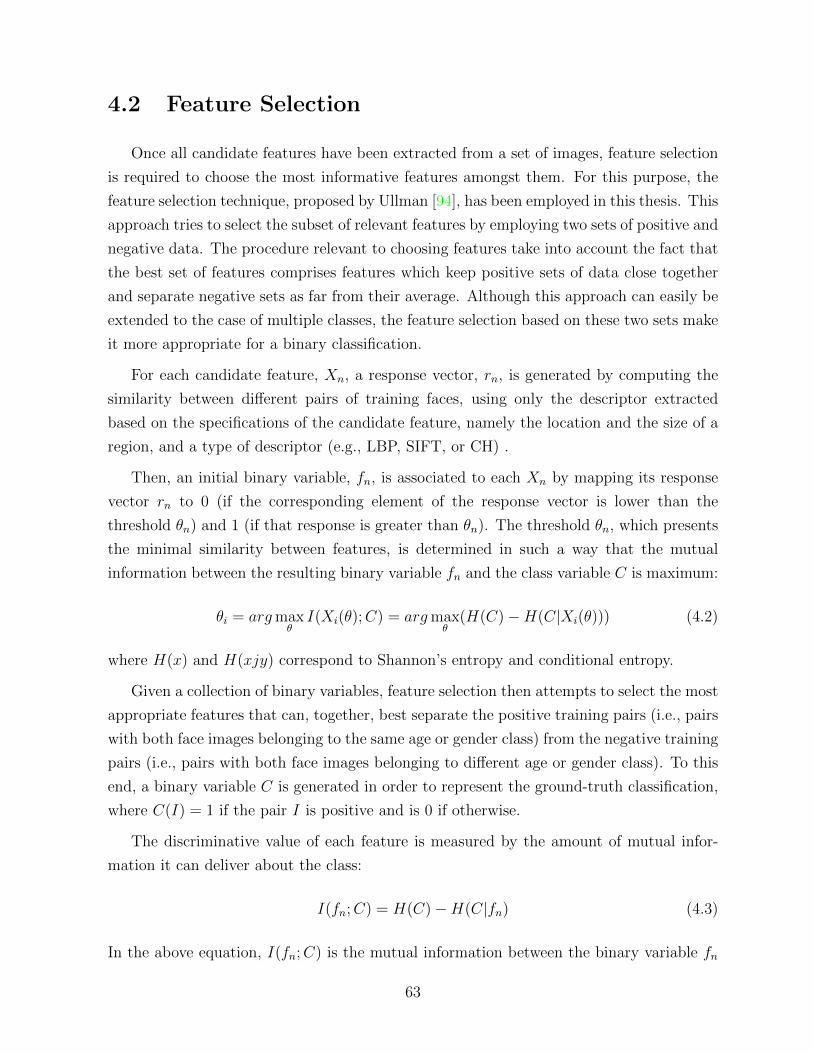
4.2 Feature Selection
Once all candidate features have been extracted from a set of images, feature selection
is required to choose the most informative features amongst them. For this purpose, the
feature selection technique, proposed by Ullman [94], has been employed in this thesis. This
approach tries to select the subset of relevant features by employing two sets of positive and
negative data. The procedure relevant to choosing features take into account the fact that
the best set of features comprises features which keep positive sets of data close together
and separate negative sets as far from their average. Although this approach can easily be
extended to the case of multiple classes, the feature selection based on these two sets make
it more appropriate for a binary classification.
For each candidate feature, Xn, a response vector, rn, is generated by computing the
similarity between different pairs of training faces, using only the descriptor extracted
based on the specifications of the candidate feature, namely the location and the size of a
region, and a type of descriptor (e.g., LBP, SIFT, or CH) .
Then, an initial binary variable, fn, is associated to each Xn by mapping its response
vector rn to 0 (if the corresponding element of the response vector is lower than the
threshold θn) and 1 (if that response is greater than θn). The threshold θn, which presents
the minimal similarity between features, is determined in such a way that the mutual
information between the resulting binary variable fn and the class variable C is maximum:
θi = argmaxθI(Xi(θ);C) = argmax
θ(H(C)−H(C|Xi(θ))) (4.2)
where H(x) and H(xjy) correspond to Shannon’s entropy and conditional entropy.
Given a collection of binary variables, feature selection then attempts to select the most
appropriate features that can, together, best separate the positive training pairs (i.e., pairs
with both face images belonging to the same age or gender class) from the negative training
pairs (i.e., pairs with both face images belonging to different age or gender class). To this
end, a binary variable C is generated in order to represent the ground-truth classification,
where C(I) = 1 if the pair I is positive and is 0 if otherwise.
The discriminative value of each feature is measured by the amount of mutual infor-
mation it can deliver about the class:
I(fn;C) = H(C)−H(C|fn) (4.3)
In the above equation, I(fn;C) is the mutual information between the binary variable fn
63

and classes C and H denote entropy. Feature selection begins by identifying the feature
whose binary variable generates the highest mutual information score. It then proceeds by
iteratively searching for the next informative feature, fr, that delivers the maximal amount
of additional information with respect to each of the previously selected features:
fr = arg maxfk∈Kr
minfj∈Sr
(I(fk, fj;C)− I(fj;C)) (4.4)
Here Kr and Sr are the set of features not yet selected, and the set of features already
selected at iteration r, respectively.
The feature selection process ends when the increment in mutual information gained
by selecting a new feature is less than a certain threshold or until the number of selected
features reaches a certain limit. It worth mentioning that selecting more features doesn’t
necessarily increase the performance of the classification process and can even contribute to
a greater degree of mis-classification. Therefore, the number of features should be tuned to
let those features with a large contribution go through the classification model and without
those having a low discriminative power.
Figures 4.6, 4.7, and 4.8 show the results of applying feature selection on texture and
shape features extracted with the purpose of discriminating age and gender classes. Red
squares in Figure 4.6 show the regions of interest (ROI’s) which the corresponding de-
scriptors have been selected as the most discriminative features for determining gender.
Similarly, Green squares in Figure 4.7 and Figure 4.8 represent those ROIs which have
been selected for age classification.
Figure 4.6: The first seven texture features selected by Ullman feature selection techniqueto classify gender subjects
64

Figure 4.7: The first seven texture features selected by Ullman feature selection techniqueto classify age subjects
Figure 4.8: The first seven shape features selected by Ullman feature selection techniqueto classify age subjects
4.3 Classification
As explained beforehand, the feature selection process provides us with a set of features
that each represent a certain region in the face image and specify a particular descriptor
type to be extracted from that region. By concatenating all of regions’ descriptors together,
a global representation of the face image is produced. A learning method must then be
applied to perform the task of classification. This learning method aims to construct a
classifier based on extracted descriptors of the training set. Among the existing methods,
the Support Vector Machine (SVM) is one of the most popular as it performs extremely
well and has an efficient open source implementation[16].
4.3.1 Support vector machine (SVM)
The Support Vector Machine(SVM) proposed by Boser et. al[10] is one of the commonly
chosen learning techniques in supervised classification processes. The training data set and
its label set is fed into the classifier. The SVM classifier then finds an optimal decision
boundary to separate the data based on its corresponding labels.
The basic form of the SVM[92] is proposed for two class problems and aims at finding
the optimal hyperline with the widest margin possible to better separate classes. This
65

margin corresponds to the distance between the hyperline and classes’ support vectors.
An example would be of Figure 4.9, which presents the two classes’ data in R2. As it is
evident, these data can be separated linearly by a hyperplane with the form of ω.x− b = 0,
where b||ω|| indicates the hyperplane’s offset.
! " # $ % & ' ( ) *
!
"
#
$
%
&
'
(
)
*
+,-./"
+,-./-"
+,-./!
Figure 4.9: Support vector Machine schema
The hyperplanes corresponding the borders of these two classes can be formulated as
ω.x − b = 1 and ω.x − b = −1, where the distances between them (”the margin”) is
equivalent to 2||ω|| . To generalize these hyperplanes so that all classes’ points fall into them
we can write them in the following form:{ω.x− b ≥ 1 ∀xi ∈ C1
ω.x− b ≤ −1 ∀xi ∈ C2
= yi(ω.x− b) ≥ 1∀xi (4.5)
Since we aim to maximize the margin space we can write:{< ω, x1 > −b ≥ 1
< ω, x2 > −b ≤ −1⇒< ω, (x1 − x2) >= 2⇒< ω
||ω||, (x1 − x2) >=
2
||ω||(4.6)
Since the SVM also aims to maximize the margin between these two classes ( 2||w||), the
term ||ω|| should be minimized. What’s more, the potential errors that can emerge when
mapping classes’ data to the hyperplane should be minimized. This means that the problem
66

of finding the hyperplane can be expressed in the Lagrange multiplier term as follows:
min(ω,b)
maxαi≥0
1
2||ω||2 −
n∑i=1
αi(yi(ω.xi − b)− 1) (4.7)
where parameter α is the Lagrange multiplier parameter. The solution to this quadratic
equation is founds as follows [51]:
ω =n∑i=1
αixiyi (4.8)
where xi values that correspond to non-zero values of αi, represents the support vectors
on the margins (on the lines yi(ω.xi − b) = 1)
From the arguments seen above, it follows that the basic SVM cannot be applied for
non-linearly separable and multi-class cases. Thus, in order to generalize this framework,
the Kernel SVM has been proposed. The Kernel SVM tackles this problem by mapping
the training data to a feature space of high dimension and then constructs a linear decision
model to separate the data classes. This highly-dimensional space is characterized by the
inner product between data and is selected in such a way that the data in this space can
be separated linearly.
As such, the Representer theorem[50] suggests that, instead of optimizing the ω value in
high-dimensional space, a set of Kuhn-Tucker coefficients (α) can be optimized as follows:
ω =n∑i=1
αiΦ(xi) (4.9)
Thus, the formula to calculate a hyperplane (the decision rule) can now be written as
follows:
F (x) =n∑i=1
αiΦ(xi).Φ(x) + b (4.10)
And the similarity kernel can be expressed as follows:
K(xi, x) = Φ(xi).Φ(x) (4.11)
which formulates our decision rule by:
F (x) =n∑i=1
αiK(xi, x) + b (4.12)
67

So the equation (4.7) is expressed as follows:
minα{1
2
∑i,j
αiαjΦ(xi).Φ(xj)−∑i
yiαi} (4.13)
where∑
i αi = 0. Similar the basic SVM, the set of non-zero αis in∑n
i=1 αiyi = 0 are
called Support Vectors(SV).
To make an appropriate nonlinear feature map, which maps data to a high-dimensional
space within which data are best separated, different kernels have been proposed. The
polynomial decision surface and Gaussian Radial Basis function (RBF) are among the
most popular kernels currently being used to achieve this purpose:
Kpoly(x, y) = (x.y + 1)d
KRBF (x, y) = βe−γ||x−y||2
(4.14)
It worth mentioning that the parameters regarding each kernels should be tuned for each
classification process.
4.4 Experimental Results
This section provides the results of the methods described earlier on two bench mark
databases. All codes are implemented in C++ using the two most popular libraries:
OpenCV 2.4.5 library (used as an open source library specialized for computer vision
applications), and LIBSVM (used as a library for Support Vector Machines)[16].
4.4.1 Dataset
The number of databases can be used for the purpose of age and gender recognition
are limited due to their number of images and the age and gender range distribution.
In general, collecting a face database which can fit to different face processing problem
is not easy due to the multiple aspects regarding the subject that should be considered.
Regarding the fact that the faces can be collected automatically or manually, different
issues are being faced. In automatic approaches, which a set of available images are being
used in constructing the database, detecting face images and labeling them is not an easy
task to do. As an example, providing some meta information or informative tags such as
age, gender, spectacles, smile, etc involves a manual and precise tagging system. Moreover,
68

data privacy policies for these images are sensitive subjects and it becomes a bigger issue
for companies who want to use them in their products. On the other hand, creating a
database manually requires a set of setups and configurations, which for some applications
like investigation of aging affect can be quite expensive. Here, the performance of the
different descriptors explained before has been evaluated with two standard benchmark
databases for age and gender recognition: the Facial Recognition Technology (FERET)
database (as was described in section 3.6.1) and the Gallagher Collection Person Dataset
(GROUPS).
The Facial Recognition Technology (FERET) database
The Color FERET is a commonly used database in the field of face processing, as it
provides information concerning, the age, the ethnicity, and gender of its faces. As previ-
ously mentioned, this database contains faces in different poses, expressions and lightening
conditions. In this section the techniques described are tested on the protocol proposed by
[6] over 1, 689 frontal face images of 969 male subjects and 720 female subject (their age
and gender information were provided) taken from Fa and Fb probes. 845 face images(360
female and 485 male) were used for training purposes and 844 face test images (484 males
and 360 female) were used to put our methods through classifier tests to ensure their
validity.
The Gallagher Collection Person Dataset (GROUPS)
The Gallagher’s database[34], which is publicly available, is composed of 28, 231 faces
collected from Flickr images taken under unconstrained conditions. Images were gathered
based on the search for four subjects: wedding, bride, groom and portrait. 86 percent of
database’s faces were detected using a face detection algorithm and other faces were added
manually. Furthermore, they have been manually labeled with the corresponding gender
and age where the age labels assigned to one of seven categories: 0-2, 3-7, 8-12, 13-19,
20-36, 37-65, and 66+. The faces are labeled based on their gender and their association
to one of seven age groups (covering from 0 to +75 years). As there was no common
and defined protocol for the experiments on this dataset, Dago-Casas et al. [3], suggested
a folding protocol using 14, 760 of the higher resolution faces and distributed them into
five folds, with an equal number of males and females in each fold. To obtain this result,
they[24] employed a face detection technique as well as an alignment method and removed
the low resolution faces. Then, they randomly removed some of the male faces so as to
69

have an equal number of male and female faces in each fold. Finally, they came up with a
framework within which each fold contains the images of 2952 people under various changes
of illumination, camera poses and image quality. It bears mentioning that Dago-Casas et
al. [24] obtained a gender classification accuracy of 86.61% by using Gabor jets (described
in 4.1.2) on this framework. Gallagher and Chen[35] had previously reported 42.9% and
74.1% accuracy for age and gender classification by using a combination of appearance and
context information. Similarly, Shan[81] had reached 50.3% and 75.7% for age and gender
classification by boosted Gabor features on this database without a common framework.
However, only Dago-Casas et al. obtained such a high level of accuracy, which was caused
by their protocols and better feature types. It worth mentioning that the age classification
results reported for this dataset are not obtained in a common framework and, therefore
we are not able to make fair comparisons.
The age and gender distribution of the whole database and the proposed framework by
Dago-Casas et al. [24] has been shown in the Table 4.1.
Table 4.1: Gender and age distribution in Groups dataset
Gender and age groups Original Gallagher’s dataset Dago-Casas et al.’s framework [3]
Male 13672 7380
Female 14559 7380
(0-2) 954 534
(3-7) 1595 906
(8-12) 872 417
(13-19) 1692 899
(20-36) 15048 7921
(37-65) 6817 3463
(66+) 1253 620
70

4.4.2 Results
In this experiment, results concerning gender and age recognition have been gathered
based on three different types of descriptors. In the Gallagher dataset, the results are
averaged over five folds of each method for both gender and age recognition rates in per-
centages(i.e. the rate of correct decisions to the number of overall decisions, which can be
interpreted as the Rank 1 identification rate). Each fold contains the images of 2952 people
under various changes of illumination, camera poses and image qualities. In addition to
this, these methods are tested on 1200 face images in the FERET dataset and consist of im-
ages taken under a variety of lightings and illustrating various expressions. Texture, shape
and color features were extracted for every image in each dataset and then concatenated
into a single feature vector. The 200 most informative feature bins amongst all resulting
vectors were selected in the Gallagher dataset. These selected features later were applied
for face representation on both Gallagher and FERET datasets. Furthermore, it was found
that applying an SVM with a RBF kernel to the database representing the selected feature
vectors begets outperformances of all other strategies [24] in terms of accuracy. The results
of Gabor Jets, raw pixel values and LBP combined with PCA are provided in last three
rows of table 4.2.
In each rows of Tables 4.2 and 4.3, CLR-LBP(XYZ) refers to the differences between
the Y value of the center of each patch and its neighboring X and Z values such that if
|Y −X| is greater than or equal to |Y −Z|, we set the neighbor’s value as ”1”. Otherwise,
it is set to ”0”.
Table 4.2 shows comparative results of gender recognition when results obtained with
different methods on FERET and Gallagher’s datasets. In all experiment the most 200
informative feature bins have been selected.
71

Table 4.2: Comparative results of the gender recognition systems on the FERET andGallagher’s datasets.
Methodgender recognition
Gallagher FERET
LBP 90.43 100
CH 82.82 76.45
Color CENTRIST 87.74 96.90
CLR-LBP(RGB) 87.95 96.90
CLR-LBP(GBR) 62.17 96.90
CLR-LBP(BRG) 61.60 51.45
CLR-LBP(HSV) 52.64 57.85
CLR-LBP(SVH) 51.65 60.12
CLR-LBP(VHS) 52.66 92.98
SIFT 89.61 100
LBP+CH+SIFT 91.59 100
LBP+CLR-LBP(RGB)+SIFT 91.94 100
Pixels+PCA 80.11[24] 96.62[70]
Gabor Jets+PCA 86.61[24] 98 [56]
LBPs+PCA 86.69[24] 95.8[57]
Appearance+context 74.1[35] N/A
boosted Gabor 75.7[81] 85[64]
To experiment with the methods for age classification described, we divided the Gal-
lagher’s dataset into three age groups, having three, five and seven age categories, respec-
tively. Similarly, we divided the FERET database into four age categories. Table 4.3 shows
comparative age recognition results for these age categories with different methods tested
on Gallagher’s dataset. In all experiment the most 200 informative feature bins have been
selected.
72
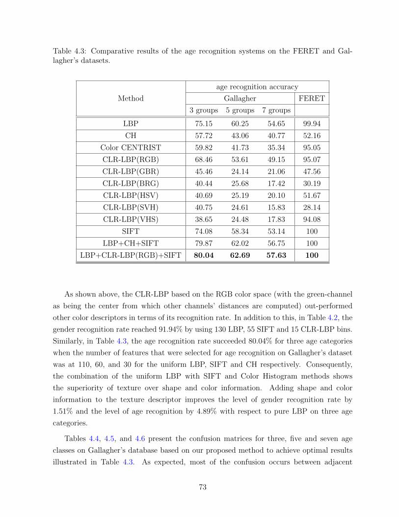
Table 4.3: Comparative results of the age recognition systems on the FERET and Gal-lagher’s datasets.
Method
age recognition accuracy
Gallagher FERET
3 groups 5 groups 7 groups
LBP 75.15 60.25 54.65 99.94
CH 57.72 43.06 40.77 52.16
Color CENTRIST 59.82 41.73 35.34 95.05
CLR-LBP(RGB) 68.46 53.61 49.15 95.07
CLR-LBP(GBR) 45.46 24.14 21.06 47.56
CLR-LBP(BRG) 40.44 25.68 17.42 30.19
CLR-LBP(HSV) 40.69 25.19 20.10 51.67
CLR-LBP(SVH) 40.75 24.61 15.83 28.14
CLR-LBP(VHS) 38.65 24.48 17.83 94.08
SIFT 74.08 58.34 53.14 100
LBP+CH+SIFT 79.87 62.02 56.75 100
LBP+CLR-LBP(RGB)+SIFT 80.04 62.69 57.63 100
As shown above, the CLR-LBP based on the RGB color space (with the green-channel
as being the center from which other channels’ distances are computed) out-performed
other color descriptors in terms of its recognition rate. In addition to this, in Table 4.2, the
gender recognition rate reached 91.94% by using 130 LBP, 55 SIFT and 15 CLR-LBP bins.
Similarly, in Table 4.3, the age recognition rate succeeded 80.04% for three age categories
when the number of features that were selected for age recognition on Gallagher’s dataset
was at 110, 60, and 30 for the uniform LBP, SIFT and CH respectively. Consequently,
the combination of the uniform LBP with SIFT and Color Histogram methods shows
the superiority of texture over shape and color information. Adding shape and color
information to the texture descriptor improves the level of gender recognition rate by
1.51% and the level of age recognition by 4.89% with respect to pure LBP on three age
categories.
Tables 4.4, 4.5, and 4.6 present the confusion matrices for three, five and seven age
classes on Gallagher’s database based on our proposed method to achieve optimal results
illustrated in Table 4.3. As expected, most of the confusion occurs between adjacent
73

classes. For instance, it is clear from the last rows of Tables 4.6 that mature adults are
often misclassified as young adult or senior classes, which is a commonly made mistake.
Table 4.4: Confusion matrix for three age classes employing feature selection on a set ofLBP, CLR-LBP(RGB) and SIFT (numbers are normalized).
XXXXXXXXXXXXXXXActual
Prediction(0-2) (3-7) (8-12) (13-19) (20-36) (37-65) (66+)
(0-2) 87.5752 9.8138 1.4749 0 0.3739 0.1887 0.5735
(3-7) 18.9652 50.350 22.8436 4.2735 1.5571 0.4082 1.6024
(8-12) 2.3331 25.4017 49.5909 11.4253 6.4858 3.3447 1.4184
(13-19) 0.6856 5.6479 15.8349 43.5546 25.0426 6.5393 2.6952
(20-36) 0.6289 2.0510 4.6446 22.7848 44.9055 19.9257 5.0595
(37-65) 0.5169 1.2761 2.3047 7.9813 21.1957 42.1779 24.5473
(66+) 0.4803 0.1575 0.6661 1.1222 2.6093 9.7136 85.2511
Table 4.5: Confusion matrix for five age classes employing feature selection on a set ofLBP, CLR-LBP(RGB) and SIFT (numbers are normalized).
XXXXXXXXXXXXXXXActual
Prediction(0-12) (13-19) (20-36) (37-65) (66+)
(0-12) 84.5187 10.4980 2.5590 1.4549 0.9694
(13-19) 13.1562 54.4231 23.8387 6.8705 1.7116
(20-36) 3.5302 25.8553 46.4744 19.6832 4.4569
(37-65) 1.8250 9.5284 21.0849 44.3041 23.2575
(66+) 0.5023 1.5804 2.1552 10.4260 85.3361
Table 4.6: Confusion matrix for seven age classes employing feature selection on a set ofLBP, CLR-LBP(RGB) and SIFT (numbers are normalized).
XXXXXXXXXXXXXXXActual
Prediction(0-19) (20-65) (66+)
(0-19) 77.5159 20.1424 2.3416
(20-65) 15.2422 73.0572 16.0605
(66+) 1.6039 8.8490 89.5470
74

In addition to the previous tests, we performed another experiment to demonstrate
that increasing the number of features would not necessarily increase recognition rate.
This experiment has been conducted on a set of features extracted by LBP for gender
recognition on Gallagher’s dataset. Result of this experiment is shown in Figure 4.10.
0 50 100 150 200 250 300 350 4000.82
0.83
0.84
0.85
0.86
0.87
0.88
0.89
0.9
0.91
accura
cy o
f gender
cla
ssific
ation
number of feature bins
Figure 4.10: Effect of the number of features selected
4.5 Conclusion
In this chapter, a novel gender and age classification method was reported. Unlike
the vast majority of the existing solutions that focus on a single visual descriptor (and,
therefore, limit the face representations by encoding only a certain characteristic of the
image regions such as shape, texture or color), this new method facilitates the integration
of multiple feature types. This allows for the taking advantage of various sources of visual
information. The proposed framework, based on the selection of informative features, only
allows the regions that can best separate face images of different demographic classes (with
respect to age and gender) to contribute to the face representations. This, in turn, improves
classification and recognition accuracies. In addition to this, a new color descriptor (CLR-
LBP) was proposed inspired by the local binary pattern schemes that was found to obtain
results comparable with those of other existing color descriptors in object recognition. A set
of experiments conducted on the challenging Gallagher’s and FERET database validated
the effectiveness of the proposed solution with regards to accurately classifying the age and
gender of face images taken under unconstrained conditions.
75
Chapter 5
Conclusion
In this thesis, we investigated two problems of the face processing field, face recognition,
and age and gender classification. We reviewed recent developments in these two fields
and our survey demonstrated that many of the existing methods suffer from difficulties in
analyzing data collected from uncontrolled environments. These difficulties stem from the
fact that, in face, gender and age recognition problems, proposing a model that allows for
an accurate recognition that can be generalized so as to apply to everyone is not an easy
task.
The first part of our research proposes a model for face recognition that employs fea-
tures extracted from sample images of uncontrolled environments to represent a face im-
age. We investigated different approaches such as dimension reduction techniques, edge
detection operators and texture and shape feature extractors to represent the face im-
age. Afterwards, these methods were evaluated on two popular databases: the FERET
database and the collected version of LFW. After evaluating these aforementioned methods
on the FERET database and the collected version of LFW, we were inspired to use the
bag-of-words method basing it on the uniform LBP features. Furthermore, we used the
”Local-Threshold” parameter in cases where the detected face is not in our database. Ex-
periments on a challenging dataset showed that our approach achieved a better accuracy in
comparison with the other popular methods such as the PCA, LDA, LBPH, SIFT, BRIEF
and FREAK methods. To tune the parameters, we conducted an extensive experiment for
which the results are provided in Section 3.6.
In the other part of our research, we presented a novel age and gender classification
method. The vast majority of the existing methods focus on a single visual descriptor,
which limits the face representations by encoding only a certain characteristic of the image
76

regions such as shape, texture or color. In contrast to this, our system facilitates the inte-
gration of multiple feature types and allows us to take advantage of various sources of visual
information. By integrating the proposed age and gender classifier with a reliable tracker
and, possibly, a face quality assessment measure (e.g. [[31]]), a real-time demographics
visual system can be built.
Additionally, a new color descriptor (CLR-LBP) was proposed, inspired by the local
binary pattern schemes [73], and was found to produce results comparable with those of
other existing color descriptors in object recognition. A set of experiments conducted on
the FERET [75] and Gallagher’s [35] database validated the effectiveness of our proposed
solution by accurately classifying the age and gender of examined subjects. Experiments
on Gallagher’s dataset, which contains images captured under various levels of changes of
illumination, camera poses and quality showed that we are able to achieve a 80.04% and
91.94% accuracy in age and gender classification - respectively - by employing different
visual features extracted from a face image.
5.1 Future Work
In light of the good results obtained by applying the feature selection method on age and
gender recognition problems, it follows that similar efforts can be employed to improve face
recognition problem. Thus, instead of using a single visual descriptor, a possible solution
would be to apply feature selection scheme on different regions of the face image. The
features that would be selected would be those that offer the most distinctive information.
This would allow us to integrate different visual feature types to represent each region of
face images.
Another limitation of the face, age and gender recognition systems is that they are all
sensitive to pose changes. Therefore, applying pose estimation to the detected faces would
give us a good sense of how each face elements corresponds to the overall face positioning.
These information can help us to better represent the face image as a whole.
Another potential future direction is to explore the possibility of using a multi-class
feature selection method rather than a binary one in order to study the level of improvement
it brings to the current accuracy of age classification approach. Building a database from
images of people captured in real-world scenarios (e.g., images from people watching a
public TV display) would be a good idea to generalize the age and gender model for
real-world applications.
77

References
[1] Probability Theory I. Graduate Texts in Mathematics. Springer, 1977.
[2] Herv Abdi, Dominique Valentin, Betty Edelman, and Alice J. O’Toole. More about
the difference between men and women: Evidence from linear neural networks and
the principal-component approach. 1995.
[3] H. Ai and Z. Yang. Demographic classification with local binary patterns. Advances
in Biometrics, 4642:464–473, August 2007.
[4] A.N. Akansu and R.A. Haddad. Multiresolution Signal Decomposition: Transforms,
Subbands, and Wavelets. Telecommunications Series. Academic Press, 2001.
[5] A. Alahi, R. Ortiz, and P. Vandergheynst. Freak: Fast retina keypoint. In Proceedings
of the 2012 IEEE Conference on Computer Vision and Pattern Recognition (CVPR),
pages 510–517, June 2012.
[6] F.A. Alomar, G. Muhammad, H. Aboalsamh, M. Hussain, A.M. Mirza, and G. Bebis.
Gender recognition from faces using bandlet and local binary patterns. In 20th
International Conference on Systems, Signals and Image Processing (IWSSIP), pages
59–62, July 2013.
[7] P.N. Belhumeur, J.P. Hespanha, and D. Kriegman. Eigenfaces vs. fisherfaces: recog-
nition using class specific linear projection. volume 19, pages 711–720, Jul 1997.
[8] S. Belongie, J. Malik, and J. Puzicha. Shape matching and object recognition using
shape contexts. volume 24, pages 509–522, Apr 2002.
[9] Wen bing Horng, Cheng ping Lee, and Chun wen Chen. Classification of age groups
based on facial features. 2001.
78
[10] Bernhard E. Boser, Isabelle M. Guyon, and Vladimir N. Vapnik. A training algorithm
for optimal margin classifiers. In Proceedings of the 5th Annual ACM Workshop on
Computational Learning Theory, pages 144–152. ACM Press, 1992.
[11] Roberto Brunelli and T. Poggio. Face recognition: features versus templates. Pattern
Analysis and Machine Intelligence, IEEE Transactions on, 15(10):1042–1052, Oct
1993.
[12] Len Bui, D. Tran, Xu Huang, and G. Chetty. Face gender recognition based on 2d
principal component analysis and support vector machine. pages 579–582, Sept 2010.
[13] J. G. Wang C. Y. Lee, J. Li and W. Y. Yau. Dense sift and gabor descriptors-based
face representation with applications to gender recognition. International Conference
on Control Automation Robotics and Vision, pages 1860–1864, December 2010.
[14] M. Calonder, V. Lepetit, M. Ozuysal, T. Trzcinski, C. Strecha, and P. Fua. BRIEF:
Computing a Local Binary Descriptor Very Fast. volume 34, pages 1281–1298, 2012.
[15] John Canny. A computational approach to edge detection. IEEE Transactions on
Pattern Analysis and Machine Intelligence, PAMI-8(6):679–698, Nov 1986.
[16] Chih-Chung Chang and Chih-Jen Lin. LIBSVM: A library for support vector ma-
chines. volume 2, pages 27:1–27:27, 2011. Software available at http://www.csie.
ntu.edu.tw/~cjlin/libsvm.
[17] Duan-Yu Chen and Po-Chiang Hsieh. Face-based gender recognition using compres-
sive sensing. pages 157–161, Nov 2012.
[18] Yu Chen, Wei-Shi Zheng, Xiaohong Xu, and Jian-Huang Lai. Discriminant sub-
space learning constrained by locally statistical uncorrelation for face recognition.
volume 42, pages 28–43, 2013.
[19] Hongrong Cheng, Zhiguang Qin, Weizhong Qian, and Wei Liu. Conditional mutual
information based feature selection. pages 103–107, Dec 2008.
[20] Wei-Ta Chu, Chih-Hao Chen, and Han-Nung Hsu. Color centrist: Embedding color
information in scene categorization. volume 25, pages 840 – 854, 2014.
[21] N.P. Costen, M. Brown, and S. Akamatsu. Sparse models for gender classification.
pages 201–206, May 2004.
79

[22] Garrison W. Cottrell and Janet Metcalfe. Empath: Face, emotion, and gender recog-
nition using holons. In Richard Lippmann, John E. Moody, and David S. Touretzky,
editors, NIPS, pages 564–571. Morgan Kaufmann, 1990.
[23] Oana G. Cula and Kristin J. Dana. 3d texture recognition using bidirectional feature
histograms. volume 59, page 2004, 2004.
[24] L. L. Yu D. Gonzalez-Jimenez, J. L. Alba-Castro and P. Dago-Casas. Single-and
cross-database benchmarks for gender classification under unconstrained settings.
IEEE International Conference on Computer Vision Workshops, pages 2152–2159,
November 2011.
[25] C. Ding and H. Peng. Minimum redundancy feature selection from microarray gene
expression data. pages 523–528, Aug 2003.
[26] Richard O. Duda and Peter E. Hart. Use of the hough transformation to detect lines
and curves in pictures. volume 15, pages 11–15, 1972.
[27] J. G. Wang E. Sung, J. Li and W. Y. Yau. Boosting dense sift descriptors and shape
contexts of face images for gender recognition. IEEE Conference on Computer Vision
and Pattern Recognition Workshops, pages 96–102, June 2010.
[28] P.A. Estevez, M. Tesmer, C.A. Perez, and J.M. Zurada. Normalized mutual informa-
tion feature selection. IEEE Transactions on Neural Networks, 20(2):189–201, Feb
2009.
[29] Kamran Etemad and Rama Chellappa. Discriminant analysis for recognition of hu-
man face images (invited paper). In Josef Bign, Grard Chollet, and Gunilla Borgefors,
editors, AVBPA, volume 1206 of Lecture Notes in Computer Science, pages 127–142.
Springer, 1997.
[30] Ehsan Fazl-Ersi, Mohammad Esmaeel Mousa Pasandi, Robert Laganiere, and Maher
Awad. Age and gender recognition using informative features of various types. In 21st
IEEE International Conference on Image Processing (ICIP), Paris, France, October
2014.
[31] Adam Fourney and Robert Laganiere. Constructing face image logs that are both
complete and concise. In CRV, pages 488–494, 2007.
[32] Xiaofeng Fu, Guojun Dai, Changjun Wang, and Li Zhang. Centralized gabor gradient
histogram for facial gender recognition. 4:2070–2074, Aug 2010.
80

[33] D. Gabor. Theory of communication. part 1: The analysis of information. Jour-
nal of the Institution of Electrical Engineers - Part III: Radio and Communication
Engineering, 93(26):429–441, November 1946.
[34] A. Gallagher and T. Chen. Clothing cosegmentation for recognizing people. In Proc.
CVPR, 2008.
[35] A.C. Gallagher and Tsuhan Chen. Understanding images of groups of people. vol-
ume 0, pages 256–263, Los Alamitos, CA, USA, 2009. IEEE Computer Society.
[36] B. A. Golomb, D. T. Lawrence, and T. J. Sejnowski. Sexnet: A neural network
identifies sex from human faces. In Proceedings of the 1990 Conference on Advances
in Neural Information Processing Systems 3, NIPS-3, pages 572–577, San Francisco,
CA, USA, 1990. Morgan Kaufmann Publishers Inc.
[37] Guodong Guo, Guowang Mu, and Yun Fu. Gender from body: A biologically-inspired
approach with manifold learning. 5996:236–245, 2010.
[38] P. Jonathon H. Wechsler, J.R.J. Huang and S. Gutta. Mixture of experts for clas-
sification of gender, ethnic origin, and pose of human faces. IEEE Transactions on
Neural Networks, 11:948–960, July 2000.
[39] Ziad M. Hafed and Martin D. Levine. Face recognition using the discrete cosine
transform. volume 43, pages 167–188, 2001.
[40] H. Hotelling. Analysis of a complex of statistical variables into principal components.
1933.
[41] P.V.C. Hough. Machine analysis of bubble chamber pictures. In Proceedings of the
International Conference on High Energy Accelerators and Instrumentation, 1959.
[42] Gary B. Huang and Vidit Jain. Unsupervised joint alignment of complex images. In
In ICCV, 2007.
[43] Gary B. Huang, Manu Ramesh, Tamara Berg, and Erik Learned-Miller. Labeled faces
in the wild: A database for studying face recognition in unconstrained environments.
Number 07-49, October 2007.
[44] David H. Hubel and Torsten N. Wiesel. Receptive fields of single neurons in the cat’s
striate cortex. volume 148, pages 574–591, 1959.
81

[45] L. Bourdev J. Malik and S. Maji. Describing people: A poselet-based approach to
attribute classification. IEEE International Conference on Computer Vision (ICCV),
pages 1543–1550, November 2011.
[46] Rabia Jafri and Hamid R. Arabnia. A survey of face recognition techniques. volume 5,
pages 41–68, 2009.
[47] A. Jain and J. Huang. Integrating independent components and linear discriminant
analysis for gender classification. pages 159–163, May 2004.
[48] F. Jurie and B. Triggs. Creating efficient codebooks for visual recognition. In Tenth
IEEE International Conference on Computer Vision, volume 1, pages 604–610 Vol.
1, Oct 2005.
[49] K. Karhunen. Uber lineare Methoden in der Wahrscheinlichkeitsrechnung. Annales
Academiae scientiarum Fennicae: Mathematica - Physica. Universitat Helsinki, 1947.
[50] George S. Kimeldorf and Grace Wahba. A correspondence between bayesian estima-
tion on stochastic processes and smoothing by splines. volume 41, pages 495–502.
The Institute of Mathematical Statistics, 04 1970.
[51] H. W. Kuhn and A. W. Tucker. Nonlinear programming. In Proceedings of the
Second Berkeley Symposium on Mathematical Statistics and Probability, pages 481–
492, Berkeley, Calif., 1951. University of California Press.
[52] Young H. Kwon and Niels Da Vitoria Lobo. Age classification from facial images.
pages 762–767, 1999.
[53] A. Lanitis. On the significance of different facial parts for automatic age estimation.
2:1027–1030 vol.2, 2002.
[54] A. Lanitis, C. Draganova, and C. Christodoulou. Comparing different classifiers for
automatic age estimation. IEEE Transactions on Systems, Man, and Cybernetics,
Part B: Cybernetics, 34(1):621–628, Feb 2004.
[55] A. Lanitis, C.J. Taylor, and T.F. Cootes. Toward automatic simulation of aging
effects on face images. IEEE Transactions on Pattern Analysis and Machine Intelli-
gence, 24(4):442–455, Apr 2002.
[56] XueMing Leng and Yiding Wang. Improving generalization for gender classification.
In 15th IEEE International Conference on Image Processing, pages 1656–1659, Oct
2008.
82

[57] Bing Li, Xiao-Chen Lian, and Bao-Liang Lu. Gender classification by combining
clothing, hair and facial component classifiers. volume 76, pages 18 – 27, 2012.
Seventh International Symposium on Neural Networks (ISNN 2010) Advances in
Web Intelligence.
[58] Chun-Ming Li, Yu-Shan Li, Qing-De Zhuang, and Zhong-Zhe Xiao. The face lo-
calization and regional features extraction. In Proceedings of 2004 International
Conference on Machine Learning and Cybernetics, volume 6, pages 3835–3840 vol.6,
Aug 2004.
[59] Zisheng Li, J. Imai, and M. Kaneko. Robust face recognition using block-based bag
of words. In 20th International Conference on Pattern Recognition (ICPR), pages
1285–1288, Aug 2010.
[60] T.C.-I. Lin and Yi-Jie Zhao. A feature-based gender recognition method based on
color information. pages 40–43, Nov 2011.
[61] Jinqing Liu and Yusheng Huang. Study of human face image edge detection based on
dm642. In 3rd IEEE International Conference on Computer Science and Information
Technology (ICCSIT), volume 8, pages 175–179, July 2010.
[62] S. Lloyd. Least squares quantization in pcm. volume 28, pages 129–137, Mar 1982.
[63] D.G. Lowe. Object recognition from local scale-invariant features. In The Proceedings
of the Seventh IEEE International Conference on Computer Vision, volume 2, pages
1150–1157 vol.2, 1999.
[64] Huchuan Lu and Hui Lin. Gender recognition using adaboosted feature. In Third
International Conference on Natural Computation, volume 2, pages 646–650, Aug
2007.
[65] Li Lu and Pengfei Shi. A novel fusion-based method for expression-invariant gender
classification. pages 1065–1068, 2009.
[66] Michael J. Lyons, J. Budynek, A. Plante, and S. Akamatsu. Classifying facial at-
tributes using a 2-d gabor wavelet representation and discriminant analysis. pages
202–207, 2000.
[67] S. Mika, G. Ratsch, J. Weston, B. Scholkopf, and K. Muller. Fisher discriminant
analysis with kernels. In Neural Networks for Signal Processing IX, 1999. Proceedings
of the 1999 IEEE Signal Processing Society Workshop., pages 41–48, Aug 1999.
83

[68] Erno Mkinen and Roope Raisamo. An experimental comparison of gender classifica-
tion methods. volume 29, pages 1544 – 1556, 2008.
[69] B. Moghaddam, C. Nastar, and A. Pentland. Bayesian face recognition using de-
formable intensity surfaces. In Proceedings of the IEEE Computer Society Conference
on Computer Vision and Pattern Recognition, pages 638–645, Jun 1996.
[70] B. Moghaddam and Ming-Hsuan Yang. Learning gender with support faces. IEEE
Transactions on Pattern Analysis and Machine Intelligence, 24(5):707–711, May
2002.
[71] Choon Boon Ng, Yong Haur Tay, and Bok-Min Goi. Vision-based human gender
recognition: A survey. volume abs/1204.1611, 2012.
[72] T. Ojala, M. Pietikainen, and T. Maenpaa. Multiresolution gray-scale and rotation
invariant texture classification with local binary patterns. volume 24, pages 971–987,
Jul 2002.
[73] Timo Ojala, Matti Pietikinen, and David Harwood. A comparative study of texture
measures with classification based on featured distributions. volume 29, pages 51 –
59, 1996.
[74] Karl Pearson. On lines and planes of closest fit to systems of points in space. volume 6,
pages 559–572, 1901.
[75] P.J. Phillips, Hyeonjoon Moon, P. Rauss, and S.A. Rizvi. The feret evaluation
methodology for face-recognition algorithms. In Proceedings of the 1997 IEEE Com-
puter Society Conference on Computer Vision and Pattern Recognition, pages 137–
143, Jun 1997.
[76] K. Ramesha and K.B. Raja. Face recognition system using discrete wavelet transform
and fast pca. In VinuV Das, Gylson Thomas, and Ford Lumban Gaol, editors,
Information Technology and Mobile Communication, volume 147 of Communications
in Computer and Information Science, pages 13–18. Springer Berlin Heidelberg, 2011.
[77] Ral Rojas. Adaboost and the super bowl of classifiers a tutorial introduction to
adaptive boosting. 2009.
[78] H. A. Rowley and S. Baluja. Boosting sex identification performance. International
Journal of Computer Vision, 71:111–119, January 2007.
84

[79] Y. Saatci and C. Town. Cascaded classification of gender and facial expression using
active appearance models. pages 393–398, April 2006.
[80] A.S. Samra, S. El Taweel Gad Allah, and R.M. Ibrahim. Face recognition using
wavelet transform, fast fourier transform and discrete cosine transform. In Circuits
and Systems, 2003 IEEE 46th Midwest Symposium on, volume 1, pages 272–275 Vol.
1, Dec 2003.
[81] Caifeng Shan. Learning local features for age estimation on real-life faces. In Pro-
ceedings of the 1st ACM International Workshop on Multimodal Pervasive Video
Analysis, MPVA ’10, pages 23–28, New York, NY, USA, 2010. ACM.
[82] J. Sivic and A. Zisserman. Efficient visual search of videos cast as text retrieval.
volume 31, pages 591–606, April 2009.
[83] G.W. Snedecor and W.G. Cochran. Statistical Methods. Number v. 276 in Statistical
Methods. Iowa State University Press, 1989.
[84] I. Sobel and G. Feldman. A 3x3 Isotropic Gradient Operator for Image Processing.
1968. Never published but presented at a talk at the Stanford Artificial Project.
[85] Ning Sun, Wenming Zheng, Changyin Sun, Cairong Zou, and Li Zhao. Gender
classification based on boosting local binary pattern. 3972:194–201, 2006.
[86] Ye Sun, Jian-Ming Zhang, Wang Liang-Min, Zhan Yong-Zhao, and Shun lin Song.
A novel method of recognizing ageing face based on ehmm. 8:4599–4604 Vol. 8, Aug
2005.
[87] Zehang Sun, G. Bebis, Xiaojing Yuan, and S.J. Louis. Genetic feature subset selection
for gender classification: a comparison study. pages 165–170, 2002.
[88] J.E. Tapia and C.A. Perez. Gender classification based on fusion of different spatial
scale features selected by mutual information from histogram of lbp, intensity, and
shap. IEEE Transactions on Information Forensics and Security, 8:488–499, March
2013.
[89] M.L. Teixeira. The Bayesian Intrapersonal/extrapersonal Classifier. Colorado State
University, 2003.
[90] Matthew Turk and Alex Pentland. Eigenfaces for recognition. volume 3, pages 71–86,
Cambridge, MA, USA, 1991. MIT Press.
85

[91] Ihsan Ullah, Muhammad Hussain, Hatim Aboalsamh, Ghulam Muhammad, An-
warM. Mirza, and George Bebis. Gender recognition from face images with dyadic
wavelet transform and local binary pattern. 7432:409–419, 2012.
[92] Vladimir Vapnik, Steven E. Golowich, and Alex Smola. Support vector method for
function approximation, regression estimation, and signal processing. In Advances
in Neural Information Processing Systems 9, pages 281–287. MIT Press, 1996.
[93] M. Varma and A. Zisserman. A statistical approach to material classification using
image patch exemplars. volume 31, pages 2032–2047, Nov 2009.
[94] M. Vidal-Naquet and S. Ullman. Object recognition with informative features and
linear classification. IEEE International Conference on Computer Vision (ICCV),
pages 281–288, October 2003.
[95] L. Wiskott, J.-M. Fellous, Norbert Kruger, and C. Von der Malsburg. Face recogni-
tion by elastic bunch graph matching. In Proceedings of the International Conference
on Image Processing, volume 1, pages 129–132 vol.1, Oct 1997.
[96] Laurenz Wiskott, Jean marc Fellous Z, and Norbert Kruger Y. Face recognition and
gender determination. 1995.
[97] Jianxin Wu and J.M. Rehg. Centrist: A visual descriptor for scene categorization.
IEEE Transactions on Pattern Analysis and Machine Intelligence, 33(8):1489–1501,
Aug 2011.
[98] A.L. Yuille, D.S. Cohen, and P.W. Hallinan. Feature extraction from faces using de-
formable templates. In Computer Vision and Pattern Recognition, 1989. Proceedings
CVPR ’89., IEEE Computer Society Conference on, pages 104–109, Jun 1989.
[99] Jianguo Zhang, M. Marszalek, S. Lazebnik, and C. Schmid. Local features and
kernels for classification of texture and object categories: A comprehensive study. In
Conference on Computer Vision and Pattern Recognition, pages 13–13, June 2006.
[100] Sanqiang Zhao, Yongsheng Gao, and Baochang Zhang. Sobel-lbp. In 15th IEEE
International Conference on Image Processing, pages 2144–2147, Oct 2008.
[101] W. Zhao, R. Chellappa, P. J. Phillips, and A. Rosenfeld. Face recognition: A lit-
erature survey. volume 35, pages 399–458, New York, NY, USA, December 2003.
ACM.
86


