Controllability Metrics and Algorithms for Complex NetworksFabio Pasqualetti, Sandro Zampieri, and Francesco Bullo

Abstract—This paper studies the problem of controlling com-plex networks, that is, the joint problem of selecting a set ofcontrol nodes and of designing a control input to steer thenetwork to a target state. For this problem (i) we propose a metricto quantify the difficulty of the control problem as a function ofthe required control energy, (ii) we derive bounds based on thesystem dynamics (network topology and weights) to characterizethe tradeoff between the control energy and the number ofcontrol nodes, and (iii) we propose a distributed strategy withperformance guarantees for the control of complex networks.In our strategy we select control nodes by relying on networkpartitioning, and we design the control input by leveragingoptimal and distributed control techniques. Our findings showfor instance that (i) if the number of control nodes is constant,then the control energy increases exponentially with the numberof the network nodes, (ii) if the number of control nodes is afixed fraction of the network nodes, then certain networks canbe controlled with constant energy independently of the networkdimension, and (iii) clustered networks may be easier to controlbecause, for sufficiently many control nodes, the control energydepends only on the controllability properties of the clusters andon their coupling strength. We validate our results with examplesfrom power networks, social networks, and epidemics spreading.

I. INTRODUCTION

Networks accomplish complex behaviors via local inter-actions of simpler units. The electrical power grid, masstransportation systems, and cellular networks are instances ofmodern technological networks, while metabolic and brainnetworks are biological examples. The ability to controland reconfigure complex networks via external controls isfundamental to guarantee a reliable and efficient networkfunctionality. Despite important advances in the theory ofcontrol of dynamical systems, several questions regarding thecontrol of complex networks are largely unexplored, as, forinstance, the relation between network topology and its degreeof controllability.

The problem of controlling complex networks consists ofthe selection of a set of control nodes, and the design of a(possibly distributed) control law to steer the network to atarget state. In this work we study the problem of controllingcomplex networks from an energy perspective. Inspired byclassic controllability notions for dynamical systems [1], [2],[3], [4], we define the energy to control a network as theworst-case energy of the control input to reach a target state.

This material is based upon work supported in part by NSF Award 1135819and in part by ARO Award W911NF-11-1-0092.

Fabio Pasqualetti is with the Mechanical Engineering Department, Univer-sity of California at Riverside, fabiopas@engr.ucr.edu .

Sandro Zampieri is with the Department of Information Engineering,University of Padova, Italy, sandro.zampieri@dei.unipd.it.

Francesco Bullo is with the Center for Control, Dynamical Sys-tems and Computation, University of California at Santa Barbara,bullo@engineering.ucsb.edu .

By combining this controllability notion with graph theory, wecharacterize tradeoffs between the energy to control a givennetwork and the number of control nodes, and we develop adistributed control strategy with performance guarantees forcomplex networks.Related work The notion of controllability of a dynamicalsystem was first introduced in [2], and it refers to the possi-bility of driving the state of a dynamical system to a specifictarget state by means of a control input. Several structuralconditions ensuring controllability have been proposed; seefor instance [1], [3], [4]. The concept of controllability hasfound recent interest in the context of complex networks,where classic methods are often inapplicable due to the systemdimension, and where a graph-inspired understanding of con-trollability rather than a matrix-theoretical one is preferable.

Controllability of complex networks is addressed in [5] byleveraging graph-theoretic tools from structured control theory[4]. In [5] the application of standard control results to realnetworks reveals that the number of control nodes is mainlyrelated to the network degree distribution, and that sparseinhomogeneous networks are most difficult to control, whiledense and homogeneous networks require only a few controlnodes. Analogous results are derived in [6] for observabilityof complex networks. The approach to controllability andobservability undertaken in [5], [6] has several shortcomings.First, the presented results are generic, in the sense that theyhold for almost every choice of the network parameters [7],but they may fail to hold if certain symmetries or constraintsare present [4, Section 15], [8]. Second, most results in[5], [6] rely on particular interconnection properties of theconsidered networks, perhaps the absence of self-loops aroundthe network nodes. In fact it follows from [4, Theorem14.2], equivalently from [9, Theorem 1], that every stronglyconnected network with self-loops is generically controllableby any single node, which contradicts the conclusions drawnin [5]. This discrepancy is underlined in [10] for the case ofbiological networks, and more generally in [11]. Third, thebinary notion of controllability proposed in [2] and adoptedin [5] does not characterize the difficulty of the control task. Inpractice, although a network may be generically controllableby any single node, the actual control input may not beimplementable due to actuator constraints and limitations.Finally, the design of the actual control input to drive anetwork to a particular state is not specified in [5], and itremains to date an outstanding problem for complex networksdue to their dimension and absence of a central controller.

We depart from [5], [6], [8], [11], and analogously from[12], [13], [14], by adopting a quantitative measure of networkcontrollability, namely the worst-case control energy, by char-acterizing tradeoffs between the difficulty of the control taskand the number of control nodes, and, finally, by proposing a

arX

iv:1

308.

1201

v1 [

cs.S

Y]

6 A

ug 2

013

distributed control strategy suitable for complex networks.A quantitative approach to network controllability has re-

cently been adopted in [15], [16], [17]. With respect to [15],although our measures of network controllability coincide, wefocus on the tradeoffs between control energy and numberof control nodes and on the design of a distributed controlstrategy, as opposed to scaling laws for the control energyas a function of the control horizon. With respect to [16] weprovide a rigorous framework for network controllability, and,in fact, our findings are aligned and mathematically supportthe discussions in [16]. Finally, with respect to [17] we adopta different network controllability measure, which we show tobe more appropriate for the control of most complex networks.Paper contributions The main contributions of this paperare threefold. First, we study network controllability froman energy perspective, which we quantify with the smallesteigenvalue of the controllability Gramian (Section II). Weshow that, if the number of control nodes is constant, thencertain controllable networks are practically uncontrollable, asthe control energy depends exponentially on the ratio betweenthe network cardinality and the number of control nodes.

Second, we characterize a tradeoff between the controlenergy and the number of control nodes (Section III). Inparticular, we derive an upper bound for the smallest eigen-value of the controllability Gramian as a function of thenumber of control nodes, and a lower bound on the numberof control nodes when the control energy is fixed. Our boundsshow, for instance, that in order to control a network withconstant energy, the number of control nodes must growlinearly with the network dimension. These results providea quantitative measure of the numerical findings in [16], andare in accordance with existing results in control theory [18].

Third, we propose the decoupled control strategy for thecontrol of complex networks (Section IV). The decoupledcontrol strategy consists of network partitioning, selection ofthe control nodes, and the design of a distributed controllaw to steer the network to a target state. We characterizethe performance of the decoupled control strategy, and weshow that, if sufficiently many control nodes are available,the energy to control a network depends only on the control-lability properties of its parts, and on their coupling strength.Conversely, we prove that certain networks admit a distributedcontrol strategy where the control energy is independent of thenetwork dimension. To the best of our knowledge, our decou-pled control strategy is novel, it constitutes a first solution forthe distributed scalable control of complex networks, and itleads to a novel notion of network controllability centrality.

Finally, we compare the effectiveness of our decoupled con-trol law with other network control methods through some ex-amples from power networks, social networks, and epidemics(Section V). Our numerical studies show that our decoupledcontrol strategy outperforms existing control techniques, whilebeing scalable in the network cardinality, and amenable todistributed implementation.

This paper contains three additional minor contributions.First, we show that the problem of selecting control nodesto maximize the trace of the controllability Gramian admitsa closed-form solution (Appendix). Second, we generalize

our results to the observability problem of complex networks(Remark 2). Third, we describe a heuristic strategy based onmodal controllability [19] to select control nodes (Remark 3).Notation The following notation is adopted throughout thepaper. For a vector v ∈ Rn, we let ‖v‖2 denote its Euclideannorm, that is,

‖v‖2 :=√vTv,

where T denotes transposition. For a matrix M ∈ Rn×n, letspec(M) denote the set of eigenvalues of M , and let

λmin(M) := min{|λ| : λ ∈ spec(M)},λmax(M) := max{|λ| : λ ∈ spec(M)}.

Let σ(M) be the set of the singular values of M , that is,

σ(M) := {λ1/2 : λ ∈ spec(MTM)}.Let σmax(M) := max{λ : λ ∈ σ(M)}. The spectral norm ofM is denoted by ‖M‖2, where

‖M‖2 := σmax(M).

For the vector valued signal s : N≥0 → Rn, we use ‖s‖2,T todenote its norm, that is,

‖s‖2,T :=

√√√√T−1∑t=0

‖s(t)‖2.

Vector norms, matrix norms, and signal norms will be distin-guished from the context.

II. NETWORK MODEL AND PRELIMINARY RESULTS

Consider a network represented by the undirected graphG := (V, E), where V := {1, . . . , n} and E ⊆ V × V arethe vertices and the edges sets, respectively. Let aij ∈ R bethe weight associated with the edge (i, j) ∈ E , and definethe weighted adjacency matrix of G as A = AT = [aij ],where aij = 0 whenever (i, j) 6∈ E . We associate a real value(state) with each node, collect the nodes states into a vector(network state), and define the map x : N≥0 → Rn to describethe evolution (network dynamics) of the network state overtime. We consider the discrete time linear and time-invariantnetwork dynamics described by the equation

x(t+ 1) = Ax(t). (1)

Controllability of the network G refers to the possibilityof steering the network state to an arbitrary configuration bymeans of external controls. We assume that a set

K := {k1, . . . , km} ⊆ Vof nodes can be independently controlled, and we let

BK :=[ek1 · · · ekm

](2)

be the input matrix, where ei denotes the i-th canonical vectorof dimension n. The network with control nodes K reads as

x(t+ 1) = Ax(t) +BKuK(t), (3)

where uK : N≥0 → R is the control signal injected into thenetwork via the nodes K. A network is controllable in T ∈ N

steps by the set of control nodes K if and only if for everystate xf ∈ Rn there exists an input uK such that x(T ) = xfwith x(0) = 0 [1]. Controllability of dynamical systems is awell-understood property, and it can be checked by differentstructural conditions [2], [3], [4]. For instance, let CK,T , withT ∈ N≥1, be the controllability matrix defined as

CK,T :=[BK ABK · · · AT−1BK

].

The network (3) is controllable in T steps by the nodes K ifand only if the controllability matrix CK,T is of full row rank.

The above notion of controllability is qualitative, and it doesnot quantify the difficulty of the control task as measured, forinstance, by the control energy needed to reach a desired state.As a matter of fact, many controllable networks require verylarge control energy to reach certain states [16]. To formalizethis discussion, define the T -steps controllability Gramian by

WK,T :=

T−1∑τ=0

AτBKBTKA

τ = CK,TCTK,T ,

where we have used the fact that A = AT. It can be easilyverified that the controllability Gramian WK,T is positivedefinite if and only if the network is controllable in T stepsby the nodes K [1].

Let the network be controllable in T steps, and let xf, with‖xf‖ = 1, be the desired final state at time T . Define theenergy of the control input uK as

E(uK, T ) := ‖uK‖22,T =

T−1∑τ=0

‖uK(τ)‖22,

where T is the control horizon. The unique control input thatsteers the network state from x(0) = 0 to x(T ) = xf withminimum energy is [1]

u∗K(t) := BTKA

T−t−1W−1K,T xf, (4)

with t ∈ {0, . . . , T − 1}. Then, it can be seen that

E(u∗K, T ) =

T−1∑τ=0

‖u∗K(τ)‖22 = xTf W−1K,Txf ≤ λ−1min(WK,T ),

(5)

where equality is achieved whenever xf is an eigenvectorof WK,T associated with λmin(WK,T ). Because the controlenergy is limited in practical applications, controllable net-works featuring small Gramian eigenvalues cannot be steeredto certain states. An example follows.

Example 1: (Controllable networks may exhibit practicallyuncontrollable states) Consider the network G with n nodes,weighted adjacency matrix A := [aij ] defined as

aij :=

{12 , if j = i− 1 and i ∈ {2, . . . , n},0, otherwise,

and control node K = {1}. Notice that the controllabilitymatrix CK,n is diagonal and nonsingular, and its i-th diagonalentry equals 2−i+1. Since AtBK = 0 for all t ≥ n, we haveWK,τ = CK,nCTK,n for all τ ≥ n, and the smallest eigenvalueof the controllability Gramian WK,τ equals 2−2n+2 for allτ ≥ n. We conclude that the network G with control nodes K

is controllable in T ≥ n steps, yet the control energy growsexponentially with the network cardinality. �

In this work we measure controllability of a network basedon the smallest eigenvalue of the controllability Gramian.With this choice we study controllability from a worst-caseperspective, looking at the target states requiring the largestcontrol energy to be reached. We conclude this section bydiscussing alternative controllability metrics.

Remark 1: (Controllability metrics) Different quantitativemeasures of controllability of dynamical systems have beenconsidered in the last years [20]. In addition to the small-est eigenvalue of the controllability Gramian λmin(WK,T ),the trace of the inverse of the controllability GramianTrace(W−1K,T ) and the determinant of the controllabilityGramian Det(WK,T ) have been proposed. It can be shownthat, while Trace(W−1K,T ) measures the average control energyover random target states, Det(WK,T ) is proportional to thevolume of the ellipsoid containing the states that can bereached with a unit-energy control input. The selection of thecontrol nodes for the optimization of these metrics is usuallya computationally hard combinatorial problem [13], for whichheuristics without performance guarantees and non-scalableoptimization procedures have been proposed [19], [21], [22].

Motivated by the relation

Trace(W−1K,T )

n≥ n

Trace(WK,T ),

the trace of the controllability Gramian Trace(WK,T ) hasalso been used as an overall measure of controllability in[23], [24], and recently in [17]. Unlike the controllabilitymetrics λmin(WK,T ), Trace(W−1K,T ), and Det(WK,T ), the se-lection of the control nodes to maximize Trace(WK,T ) admitsa closed-form solution (see Appendix). Unfortunately, themaximization of Trace(WK,T ) does not automatically ensurecontrollability and, as we show in Sections IV-C and V, it oftenleads to a poor selection of the control nodes with respect tothe worst-case control energy to reach a target state. �

III. CONTROL NODES AND CONTROL ENERGY

In this section we characterize a tradeoff between thenumber of control nodes and the energy required to drivea network to a target state. A matrix M is Schur stable ifλmax(M) < 1. We start with the following preliminary result.

Lemma 3.1: (Bounds on the smallest eigenvalue of thecontrollability Gramian) Consider a network G = (V, E) with|V| = n, weighted adjacency matrix A = AT, and control setK. Assume that A is Schur stable. For all T ∈ N>0 it holds

λmin(WK,T ) ≤ λmin(WK,∞) ≤ λmin(WK,T ) +λ2Tmax(A)

1− λ2max(A).

Proof: The statement follows from the definition ofcontrollability Gramian. In fact,

WK,∞ =

∞∑τ=0

AτBKBTKA

τ =WK,T +

∞∑τ=T

AτBKBTKA

τ .

Since∑∞τ=T A

τBKBTKA

τ is positive semi-definite, we haveλmin(WK,T ) ≤ λmin(WK,∞). Notice moreover that

λmin(WK,T ) = minx∈Rn

xT (WK,∞ −∑∞τ=T A

τBKBTKA

τ )x

xTx

≥ minx∈Rn

xTWK,∞xxTx

+ minx∈Rn

xT (−∑∞τ=T AτBKBTKA

τ )x

xTx

= λmin(WK,∞)− maxx∈Rn

xT (∑∞τ=T A

τBKBTKA

τ )x

xTx

= λmin(WK,∞)−∥∥∥∥∥∞∑τ=T

AτBKBTKA

τ

∥∥∥∥∥2

≥ λmin(WK,∞)− λ2Tmax(A)

1− λ2max(A),

which yields the thesis.We now derive a bound on the smallest eigenvalue of thecontrollability Gramian for a given set of control nodes.

Theorem 3.2: (Control energy and number of controlnodes) Consider a network G = (V, E) with |V| = n, weightedadjacency matrix A, and control set K. Assume that A is Schurstable. For all T ∈ N>0 it holds

λmin(WK,T ) ≤ min

1− λ2Tmin(A)

1− λ2min(A),λ2(d n

|K|e−1)max (A)

1− λ2max(A)

. (6)

Proof: We start by showing the first part of the inequal-ity. Notice that for all T ∈ N>0 it holds λmin(WK,T ) ≤λmin(WV,T ). In fact, K ⊆ V , and the control energy cannotincrease by adding control nodes to a given control set. Then,

λmin(WK,T ) ≤ λmin(WV,T ) = λmin

(T−1∑τ=0

A2τ

)

=1− λmin(A)2T

1− λmin(A)2.

We now show the second part of the inequality. Let Tmax =⌈n|K|

⌉− 1. Notice that rank(CK,Tmax) < n. In fact, CK,Tmax ∈

Rn×m with

m = Tmax|K| <(n

|K| + 1

)|K| − |K| = n.

Consequently, WK,T = CK,TmaxCTK,Tmaxis singular, and

λmin(WK,Tmax) = 0. The claimed statement follows fromLemma 3.1 by using T = Tmax.

In Theorem 3.2 we provide an upper bound on the smallesteigenvalue of the controllability Gramian or, equivalently, alower bound on the worst-case energy needed to control anetwork to an arbitrary target state, as a function of thenumber of control nodes. The bounds in Theorem 3.2 are tobe regarded as performance limitations: independently of thecontrol strategy adopted by the control nodes, the least amountof energy needed to steer the network to any unit-norm stateis bounded by the expressions in Theorem 3.2.

0.3 0.4 0.5 0.6 0.7 0.8 0.9 1−3

−2.5

−2

−1.5

−1

−0.5

0

0.5

1

⇢ = 0.75 |K|n

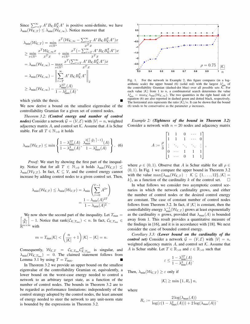
Fig. 1. For the network in Example 2, this figure compares (in a log-arithmic scale) the upper bound (6) (solid red) with the largest λ∗min ofthe controllability Gramian (dashed-dot blue) over all possible sets K. Foreach value |K| from 1 to n, a combinatorial search determines the valueλ∗min = maxK λmin(WK,∞). The two quantities in the right hand side ofequation (6) are also reported in dashed green and dotted black, respectively.The horizontal axis represents the ratio |K|/n. It can be shown that the bound(6) tends to be conservative as the parameter ρ increases.

Example 2: (Tightness of the bound in Theorem 3.2)Consider a network with n = 20 nodes and adjacency matrix

A :=ρ

3

1 1 0 · · · 11 1 1 · · · 0...

. . . . . . . . ....

0 · · · 1 1 11 · · · 0 1 1

,

where ρ ∈ (0, 1). Observe that A is Schur stable for all ρ ∈(0, 1). In Fig. 1 we compare the upper bound in Theorem 3.2with the value max{λmin(WK,T ) : K ⊆ {1, . . . , 12}, |K| =k}, as a function of the cardinality k of the control set. �

In what follows we consider two asymptotic control sce-narios in which the network cardinality grows, and eitherthe number of control nodes or the desired control energyare constant. The case of constant number of control nodesfollows from Theorem 3.2. In fact, if |K| is constant, then thecontrollability energy λ−1min(WK,T ) grows at least exponentiallyas the cardinality n grows, provided that λmax(A) is boundedaway from 1. This result provides a quantitative measure ofthe findings in [16], and it is in accordance with [18]. We nextconsider the case of bounded control energy.

Corollary 3.3: (Lower bound on the cardinality of thecontrol set) Consider a network G = (V, E) with |V| = n,weighted adjacency matrix A, and control set K. Assume thatA is Schur stable. Let T ∈ R>0 and ε ∈ R>0 such that

ε ≤ 1− λ2Tmin(A)

1− λ2min(A).

Then, λmin(WK,T ) ≥ ε only if

|K| ≥ min {1, Rε}n,

where

Rε :=2 log(λmax(A))

log(ε(1− λ2max(A))) + 2 log(λmax(A)).

Proof: From Theorem 3.2 it follows that λmin(WK,T ) ≥ εonly if

ε(1− λ2max(A)

)≤ λ2(dn/|K|e−1)max (A),

or, equivalently, only if |K| ≥ Rεn.Corollary 3.3 implies that, in order to guarantee a certain

bound on the control energy, the number of control nodes mustbe a linear function of the total number of nodes, provided thatλmax(A) is bounded away from 1 as the cardinality n grows(see Remark 4 for a discussion of the case λmax(A) = 1).Instead, classic controllability [2], [5] is (generically) ensuredby the presence of a single control node, independently of thenetwork dimension [4, Theorem 14.2], [9, Theorem 1].

Remark 2: (Observability of Complex Networks) The ob-servability problem of complex networks consists of selectinga set of sensor nodes and designing an estimation strategyto reconstruct the network state from measurements collectedby the sensor nodes [6]. Our quantitative analysis of thecontrollability of complex networks in Section III, and ourdecoupled control strategy in Section IV can be directlyapplied to the problem of observability of complex networks.To see this, define the T -steps observability Gramian by

OK,T :=

T−1∑τ=0

AτCTKCKA

τ ,

where K denotes the set of sensor nodes, and CK := BTK. The

energy associated with the network state x with sensor nodesK and observation horizon T is

E(x, T ) :=

T−1∑τ=0

‖yK(τ)‖22 = xTOK,Tx ≥ λmin(OK,T ),

where yK : N≥0 → R contains the measurements taken bythe observing nodes K [25]. Thus, the smallest eigenvalueof the observability Gramian is a suitable metric to measureobservability of a network. Since we focus on undirectednetworks where A = AT, it holds OK,T = WK,T , and theresults in Section III are readily applicable to the networkobservability problem. For instance, from Theorem 3.2 weconclude that the observability of a network, that is thesmallest eigenvalue of the observability Gramian, decreasesexponentially fast as the ratio between the network cardinalityand the number of sensor nodes grows. �

IV. DECOUPLED CONTROL OF COMPLEX NETWORKS

In this section we provide a solution to the problem ofcontrolling a complex network, that is, the problems of bothselecting the control nodes, and designing a distributed controllaw to drive the network to a target state. Our approachis different from classic solutions, as it exploit the networkstructure to jointly select the control nodes and to design acontrol law amenable to distributed implementation.

The problem of selecting control nodes in a dynamicalsystem to optimize a controllability metric is a classic controlproblem [21]. Most existing solutions either rely on combina-torial or non-scalable optimization techniques, being thereforenot suited for large networks [22], or are heuristic, in that theyexploit the specific structure of the system at hand, and do not

offer guarantees on the control energy [19], [21], [26], [27].See Remark 3 for a heuristic method to select control nodes.

A. Setup and definition of the decoupled control strategy

Our decoupled control strategy can be divided into threeparts: (i) network partitioning, (ii) selection of the controlnodes, and (iii) definition of the decoupled control law.Network partitioning Consider an undirected network G :=(V, E) with weighted (symmetric) adjacency matrix A :=[aij ]. Partition V into N disjoint sets P := {V1, . . . ,VN},and let Gi := (Vi, Ei) be the i-th subgraph of G with verticesVi and edges Ei := E ∩ (Vi×Vi).1 According to this partition,and possibly after relabeling states and inputs, the networkmatrices read as

A =

A1 · · · A1N

......

...AN1 · · · AN

, BK =

BK1· · · 0

.... . .

...0 · · · BKN

, (7)

where Ki ⊆ Vi for all i ∈ {1, . . . , N}, and the networks dy-namics can be written as the interconnection of N subsystemsof the form

xi(t+ 1) = Aixi(t) +∑j∈Ni

Aijxj(t) +BKiuKi

(t), (8)

where i ∈ {1, . . . , N} and Ni := {j : Aij 6= 0}.Selection of the control nodes For a network G := (V, E)with partition P := {V1, . . . ,VN}, we say that a node i ∈ Vkis a boundary node if aij 6= 0 for some node j ∈ V`, withk, ` ∈ {1, . . . , N} and k 6= `. Let Bi ⊆ Vi be the set ofboundary nodes in the i-th cluster, and let B =

⋃Ni=1 Bi be

the set of all the boundary nodes of the partition. We selectthe set of control nodes K = K1 ∪ · · · ∪ KN to satisfy Bi ⊆Ki ⊆ Vi for all i ∈ {1, . . . , N}, and so that each pair (A,Bi)is controllable. See Fig. 2 for an example.The decoupled control law For a network G := (V, E) withpartition P := {V1, . . . ,VN}, let xTf :=

[xTf1 · · · xTfN

]be

the target state, where ‖xf‖2 = 1, and xfi ∈ R|Vi| for i ∈{1, . . . , N}. Let ‖xf,i‖2 = αi, and notice that

∑Ni=1 α

2i = 1.

Define the control input uKiby

uKi(t) := BT

KiAT−t−1i W−1i,Txfi︸ ︷︷ ︸

vi(t)

−∑j∈Ni

BTKiAijxj(t)︸ ︷︷ ︸fij(t)

, (9)

where, with a slight abuse of notation, Wi,T is the i-thcontrollability Gramian defined by

Wi,T :=

T−1∑τ=0

AT−τ−1i BKiBTKiAT−τ−1i ,

and the control horizon T is chosen large enough so thatWi,T

is positive definite for all i ∈ {1, . . . , N}. We refer to theabove control law as to the decoupled control law.

Before analyzing the performance of our decoupled controllaw, we discuss its implementation properties. First, notice thatthe control input uKi is the sum of an open-loop control signal

1Several methods are available to partition a network [28], such as spectralmethods and modularity based heuristics. In Section V-A we employ a spectralmethod based on the Fiedler eigenvector to partition a network.

vi, and a feedback control signal∑j∈Ni

fij . Second, if eachcluster is equipped with a control center, then our decoupledcontrol law can be implemented via distributed computationby the control centers. In fact, the control signal vi dependson the dynamics of only the i-th cluster, and the feedbackcontrol signals fij can be determined upon communicationof the i-th control center with its neighboring control centersbelonging to Ni. Third and finally, our decoupled control lawis scalable, in the sense that the complexity of the control lawdoes not depend upon the network cardinality, but only onits partition, provided that the degree of each cluster remainsbounded. We further discuss this property in Sections IV-Cand V via numerical examples.

B. Analysis of the decoupled control law

We start our analysis by noticing that the decoupled controllaw (9) steers the network to the target state xf. In fact, fromequation (8) and the definition of fij in equation (9), thenetwork dynamics with decoupled control law can be writtenas the collection of N decoupled subsystems

xi(t+ 1) = Aixi(t) +BKivi(t), i ∈ {1, . . . , N}. (10)

Since vi in equation (9) equals the minimum energy input todrive the i-th subsystem (10) from xi(0) = 0 to xi(T ) = xfi,we conclude that x(T ) = xf.

We next study the energy properties of our decoupledcontrol law. Observe that the state evolution of the i-th clustercan be written as

xi(t) =

t−1∑τ=0

At−τ−1i BKiBTKiAT−τ−1i W−1i,Txfi.

For the ease of notation we assume that the matrix Ai isSchur stable for all i ∈ {1, . . . , N}. Observe that, if A is Schurstable and nonnegative, then each matrix Ai is Schur stableand λmax(Ai) ≤ λmax(A). We define the local energy matrixΛ ∈ RN×N and the L2 gains matrix Γ ∈ RN×N by

Λ := diag(λ−1min(W1,T ), . . . , λ−1min(WN,T )), (11)

Γ :=

1 γ12 · · · γ1Nγ21 1 · · · γ2N

......

. . ....

γN1 γN2. . . 1

, (12)

where γij , for i, j ∈ {1, . . . , N} and i 6= j, is the L2 gain ofthe input-output system (Aj , BKj

, BTKiAij) or, equivalently,

the H∞ gain of the transfer matrix BTKiAij(zI − Aj)−1BKj

[29].Theorem 4.1: (Energy of the decoupled control law) Con-

sider a network G = (V, E) with weighted adjacency matrixA = AT, control set K, and partition P . Assume that A isSchur stable, and that K contains all boundary nodes of P .The decoupled control law ud

K with control horizon T satisfies

E(udK, T ) ≤ ‖ΓΛ1/2‖22, (13)

where Λ and Γ are the local energy matrix and the L2 gainsmatrix defined in (11) and (12), respectively.

Proof: Let xfi be the target state of the i-th cluster, andlet ‖xfi‖2 = αi. From equations (5) and (9), and from thedefinition of L2 gain [29] it follows that

‖vi‖2,T ≤αi

λ1/2min (Wi,T )

, ‖fij‖2,T ≤γijαj

λ1/2min (Wj,T )

.

Moreover, due to the triangle inequality, we have

‖ui‖2,T ≤ ‖vi‖2,T +∑j∈Ni

‖fij‖2,T

≤ αi

λ1/2min (Wi,T )

+∑j∈Ni

γijαj

λ1/2min (Wj,T )

= ΓiΛ1/2α,

where Γi is the i-th row of Γ defined in (12), and α is thevector of αi with i ∈ {1, . . . , N}. By using (12) and the factthat ‖ud

K‖22,T =∑Ni=1 ‖ui‖22,T , we obtain

‖udK‖22,T ≤ max

‖α‖=1αTΛ1/2ΓTΓΛ1/2α = λmax

(Λ1/2ΓTΓΛ1/2

),

from which the statement follows.In Theorem 4.1 we derive a bound on the energy needed

to control a network via our decoupled control law. Theorem4.1 has several general consequences which we now describe.First, due to equation (5), if the set K of control nodes includesthe boundary nodes of a network partition P , then

λmin(WK,T ) ≥ 1

‖ΓΛ1/2‖22, (14)

where Λ and Γ are the local energy matrix and the L2

gains matrix for the partition P . This bound on the smallesteigenvalue of the controllability Gramian is novel (see [30]),and it highlights that the controllability of a clustered networkdepends on the controllability of the isolated clusters via thematrix Λ, and on their interconnections strength via the L2

gains matrix Γ. Second, the control energy for our decoupledcontrol law does not depend on the cardinality of the wholenetwork. In fact, notice that

‖ΓΛ1/2‖22 ≤ ‖Γ‖22‖Λ‖2 ≤ ‖Γ‖1‖Γ‖∞‖Λ‖∞, (15)

and that, independently of the network dimension, ‖Γ‖1 and‖Γ‖∞ remain bounded if, for instance, the network weightsand the nodes degrees are bounded. A related example is inSection IV-C. Third and finally, since the energy to controla network via the decoupled control law depends on localproperties of the network partitions, an appropriate partitioningmethod may be developed to optimize the performance of thedecoupled control law. To this aim, we state the followingcorollary of Theorem 4.1, where we derive a bound onthe control energy for our decoupled control law, which isproportional to the interconnection strength among clusters.Let ∆ be the symmetric interconnection matrix defined by

∆ :=

1 ‖A12‖2 · · · ‖A1N‖2

‖A21‖2 1 · · · ‖A2N‖2...

.... . .

...‖AN1‖2 ‖AN2‖2 · · · 1

. (16)

Corollary 4.2: (Bound for network partitioning) Let γij bethe L2 gain of the system (Aj , BKj , B

TKiAij), and let λmax =

max{λmax(Ai) : i ∈ {1, . . . , N}} < 1. Then,

γij ≤‖Aij‖2

1− λmax, for j ∈ {1, . . . , N} \ {i},

and, being T the control horizon,

E(udK, T ) ≤ ‖Λ‖∞‖∆‖

2∞

(1− λmax)2,

where Λ is the local energy matrix defined in equation (11),and ∆ is the interconnection matrix defined in equation (16).

Proof: Recall that γij equals the H∞ gain of the transfermatrix of the system (Aj , BKj , B

TKiAij), that is,

γij :=∥∥BTKiAij(zI −Aj)−1BKj

∥∥H∞

,

where ‖·‖H∞denotes the H∞ norm [29]. Since the H∞ norm

satisfies the submultiplicative property, we have

γij ≤∥∥BTKi

∥∥H∞‖Aij‖H∞

∥∥(zI −Aj)−1∥∥H∞

∥∥BKj

∥∥H∞

.

Notice that the H∞ norm of a constant transfer matrixcoincides with its induced 2-norm. Finally we have

∥∥BTKi

∥∥2

=∥∥BKj

∥∥2

= 1, and∥∥(zI −Aj)−1∥∥H∞

:= maxθ

σmax((e−iθI −Aj)−1

)= max

θ

[λmax

((eiθI −Aj)−1(e−iθI −Aj)−1

)]1/2= max

θ

[λmax

(I − 2 cos(θ)Aj +A2

j )−1)]1/2

=1

1− λmax(Aj)≤ 1

1− λmax,

from which the first part of the statement follows. The secondstatement follows from (13) and (15) and from the fact that‖Γ‖∞ ≤ ‖∆‖∞ and ‖Γ‖1 ≤ ‖∆‖1 = ‖∆‖∞.

Analogously to equation (14), from Corollary 4.2 we con-clude that, if the set K of control nodes includes the boundarynodes of a network partition P , then

λmin(WK,T ) ≥ (1− λmax)2

‖Λ‖∞‖∆‖2∞,

where Λ and ∆ are the local energy matrix and the intercon-nection matrix for the partition P , respectively, and λmax is abound on the spectral radius of the clusters of P .

We conclude this part by noting that our results lead toa novel notion of network controllability centrality,2 wherenetwork nodes are ranked according to the product of theirlocal controllability degree and their interconnection strengthwith neighboring nodes. Our notion of network controllabilitycentrality is motivated by Corollary 4.2, where the controlenergy is bounded by the scaled product of the worst-casecontrol energy of the isolated clusters ‖Λ‖∞ (least controllablecluster), and the worst-case clusters interconnection strength‖∆‖∞ (strongest interconnection strength). A comparisonbetween controllability centrality and other centrality notionsis left as the subject of future research.

Fig. 2. A circulant network with n = 24 nodes. The network is partitionedinto N = 6 clusters with nb = 4 nodes each. Controlled nodes are in black.

2 4 6 8 10 12 14 16 18 20−40

−30

−20

−10

0

N2 4 6 8 10 12 14 16 18 20

−40

−30

−20

−10

0

nb

Fig. 3. In this figures we study circulant networks partitioned as in SectionIV-C, and we compare (in a logarithmic scale) the performance of ourdecoupled control law against the minimum energy control law. In the leftfigure we maintain constant the number of nodes in each cluster, and wereport as a function of the number clusters (see Section IV-C) (i) the smallesteigenvalue of the controllability Gramian with T = ∞ and boundary nodesas control nodes (solid red), (ii) the bound (14) for the energy performance(see Theorem 4.1) achieved by our decoupled control law (dashed blue), and(iii) the smallest eigenvalue of the controllability Gramian with T =∞ andcontrol nodes selected randomly (dashed-dotted green). Notice that the energyneeded by our decoupled control law remains constant when the networkcardinality grows (the number of control nodes grows as 2N and that thenumber of nodes in each cluster remains constant). This property is notmaintained if the control nodes are chosen randomly. In the right figure wereport the same quantities as in the left figure, while maintaining constantthe number of clusters and letting the number of nodes in each cluster grow.Notice that the smallest eigenvalue of the controllability Gramian and ourbound (14) degrade with the same rate, while randomly selected control nodesrequire more energy.

C. An example of network control via decoupled control law

In this section we demonstrate our technique to control largenetworks with an example. Consider a circulant network Gwith n = nbN nodes, nb, N ∈ N, and adjacency matrix as inExample 3.2 with ρ = 0.5. We partition G into N clusters, sothat each cluster contains nb nodes. In particular, we label thenodes in increasing order, and for i ∈ {1, . . . , N} we definethe i-th cluster to have vertices Vi := {(i−1)nb+1, (i−1)nb+2, . . . , inb} and control nodes Ki := {(i− 1)nb + 1, inb}.

See Fig. 2 for an example with nb = 4 and N = 6. Itcan be numerically verified3 that the set K of control nodes isoptimal, in the sense that it solves the maximization problem

maxK⊆{1,...,n}

λmin(WK,∞),

subject to |K| = 2N.(17)

In Fig. 3 we validate Theorem 4.1 and equation (14). Noticethat, although conservative, our bound (14) captures the factthat circulant networks can be driven with constant energyto any (unit norm) target state independently of the networkdimension; this result is compatible with our analysis in Theo-rem 3.2 and in Section IV-B. Moreover, our decoupled controllaw is a distributed control law achieving this performance.Finally, it can be shown that for circulant networks, and in

2Network centrality is a fundamental concept in network analysis [31].3Due to computational complexity, we have solved the maximization

problem (17) for the cases nb = 4 and N ∈ {2, . . . , 6}.

Algorithm 1: Selection of the control nodesInput : Network G := (V, E), Number of control nodes m;Output : Control nodes K;

1 Define an empty set of control nodes K := ∅;2 Initialize trivial partition P := V with no boundary nodes Bf := ∅;

while |K| < m do3 Select least controllable cluster

` = argmin{λmin(Wi,T ) : i ∈ {1, . . . , |P|}} ;4 Compute Fiedler two-partition Pf of `-th cluster;5 Compute boundary nodes Bf of Pf;6 Update partition P with Pf;7 Update control nodes with boundary nodes K = K ∪ Bf;

8 if |K| > m then Remove boundary nodes of last partition K = K\Bf;9 if |K| < m then Add m− |K| control nodes to K as in Remark 3;

10 return K;

fact for all d-dimensional torus networks, the diagonal entriesof (I−AAT)−1 are all equal to each other. Thus, the selectionof the control nodes for the maximization of the trace of theGramian is in this case equivalent to a random positioning ofthe control nodes (see the Appendix).

V. EXAMPLES OF CONTROL OF COMPLEX NETWORKS

The main purpose of this section is to illustrate the ef-fectiveness of our decoupled control law to control complexnetworks. To this aim, we first develop a method to select thecontrol nodes based on network partitioning, and then comparethe performance of the decoupled control law with alternativecontrol schemes. The design of optimal partitioning algorithmsto minimize the energy of the decoupled control law, and athorough comparison with existing partitioning methods [28]are beyond the scope of this work.

A. Selection of the control nodes

For a connected network G := (V, E) with weighted adja-cency matrix A = AT, let Pf := {V1,V2} be the two-partitionof G determined by its Fiedler eigenvector [28], [32],4 andlet Bf be the boundary nodes of the partition Pf. Our methodto select control nodes in a connected network is describedin Algorithm 1. Loosely speaking, our method consists ofrecursively computing Fielder partitions of subnetworks ofG, and selecting the boundary nodes of each partition ascontrol nodes. Notice that (i) the algorithm repetitively selectscontrol nodes in the least controllable cluster to improve localcontrollability (line 3), (ii) the set of control nodes contains theboundary nodes of a network partition (lines 4, 5, 7), so thatour decoupled control law can be implemented, and (iii) theset of control nodes K is increasing throughout the executionof the algorithm. Consequently, the smallest eigenvalue ofthe controllability Gramian is nondecreasing throughout theexecution of the algorithm. In the last part of the algorithm(line 9) remaining control nodes are assigned according to a

4Let vf be the Fiedler eigenvector of the network Laplacian matrix. Thetwo-partition determined by vf is uniquely determined by the sign of theentries of vf [28].

heuristic procedure. Notice that Algorithm 1 may return a setof control nodes from which the network is not controllable.However, if each cluster is connected and every diagonal entryof the network matrix is nonzero, then, due to the genericityof the controllability property [4, Theorem 14.2], [9, Theorem1], each cluster as well as the whole network are genericallycontrollable by K.

Remark 3: (Heuristic selection of control nodes) Differentmethods can be used to select control nodes in a network.Combinatorial methods, heuristic procedures, or random selec-tion methods should be employed depending on the networkdimension and the available computational power. We proposethe following heuristic method inspired by the notion of modalcontrollability [19] to select control nodes within each cluster.

For a network with symmetric weighted adjacency matrixA, let V = [vij ] be the orthonormal matrix of eigenvectorsof A. The entry vij is a measure of the controllability of themode λj(A) from the control node i. In fact, an application ofthe classic PBH test to symmetric matrices shows that vij = 0implies that the mode λj(A) is not controllable from node i[1]. By extension, if vij is small, then the j-th mode is poorlycontrollable from node i. Let φi =

∑nj=1(1− λ2j (A))v2ij , and

notice that φi is a scaled measure of the controllability ofall n modes λ1(A), . . . , λn(A) from the control node i. Weheuristically select the set K of control nodes to maximizethe smallest controllability parameter φi, that is, the set K ofcontrol nodes is the solution to the maximization problem

maxK⊆{1,...,n}

min {φ1, . . . , φk},

subject to |K| = k,(18)

for a given cardinality k ∈ N. We remark that our heuristic iscomputationally as hard as computing the matrix V for eachcluster, as the maximization problem (18) can be solved bysimply ordering the controllability parameters φi. �

B. Illustrative examples

In this section we validate our method to control complexnetworks with three examples from power networks, socialnetworks, and epidemics spreading.Power network We consider a network of n generators,and we describe the dynamics of the i-th generator by thelinearized swing equation [33]

miδi + diδi = −∑j∈Ni

kij(δi − δj),

where, for the i-th generator, mi > 0 and di > 0 are the inertiaand damping coefficients, δi : R→ R[0,2π] is the phase angle,and kij is the susceptance of the power line (i, j). As in [34]we assume that mi/di � 1, and we approximate the generatordynamics with a first-order equation. Finally, we discretizethe network by using the Euler method with discretizationaccuracy h, so that the dynamics of the i-th generator read as

δi(t+ 1) = δi(t)−h

di

∑j∈Ni

kij(δi(t)− δj(t)).

For our numerical study we consider the standard IEEE 118bus system with numerical parameters taken from [35]. We

assume that every bus is connected to a generator, and we letthe discretization accuracy be h = 10−7. The results of thisnumerical study are in Fig. 5(a).Social network Inspired by the seminal work [37], the opiniondynamics of a group of individuals forming a network G =(V, E) can be modeled by the consensus system

x(t+ 1) = Ax(t),

where x : N→ R is the vector of the individual opinions, andthe matrix A = [aij ] is row stochastic and satisfies aij = 0whenever the edge (i, j) is not in the edge set E . Besidesthe description of opinion dynamics, consensus models havefound broad applicability in several domains [38].

For our numerical study we consider the social networkdescribing the Klavzar bibliography (see Fig. 4(b)), and weconstruct a consensus system by assigning a random nonzeroweight to each edge in the network. The results of thisnumerical study are in Fig. 5(b).

Remark 4: (Controllability of consensus networks) Con-nected consensus networks feature a simple unit eigenvalue[38], so that the controllability Gramian is not defined for theinfinite control horizon, as the series

∑∞τ=0A

τBKBTKA

τ isnot convergent. On the other hand, it can be shown that theunit eigenvalue is controllable at T = ∞ by any nonemptyset of control nodes with zero energy. Then, without lossof generality, the infinite horizon controllability Gramian ofconsensus networks can be defined by restricting the dynamicsto the subspace orthogonal to the consensus space, where thematrix A is Schur stable. �Epidemics spreading The N-intertwined SIS model for thedynamics of a viral infection over a network with n nodesand adjacency matrix A = [aij ] reads as [39]

pi = −αipi + (1− pi)βi∑j∈Ni

aijpj , i ∈ {1, . . . , n},

where pi : R≥0 → R[0,1] is the map describing the infectionprobability of node i, and αi ∈ R≥0, βi ∈ R≥0 are thecuring and infection rates of the i-th node. It is known that,for certain values of the ratios αi/βi, an initial infection p(0)may spread to all the nodes in the network or converge tozero. We consider the simplified model

pi = −αipi + βi∑j∈Ni

aijpj , (19)

which is a good approximation of the N-intertwined SIS modelat the initial phase of the epidemics spreading when pi(t) aresmall. We discretize the system (19) as

pi(t+ 1) = (1− hαi)pi(t) + hβi∑j∈Ni

aijpj(t), (20)

where h ∈ R>0 is a sufficiently small discretization parameter,and we study the problem of controlling the spreading of theinfection throughout the network.5

For our numerical study we consider the Pajek socialnetwork GD99c (see Fig. 4(c)), we let h = 10−2, and weselect the parameters αi and βi randomly so that the network

5An infection can be controlled by, for instance, distributing vaccines.

(20) is unstable. Due to the instability of the network, we selecta finite control horizon of n/2 control steps. The results of thisnumerical study are in Fig. 5(c).

From our numerical analysis we draw the following con-clusions. First, the smallest eigenvalue of the controllabilityGramian increases abruptly when the number of control nodesovercomes a certain threshold, or, equivalently, the controlenergy decreases abruptly when the number of control nodesovercomes a certain threshold. This phenomena is alignedwith the numerical controllability transition identified in [16]via numerical simulation. Second, our decoupled control lawoutperforms the control strategies dictated by the optimizationof the trace of the controllability Gramian and by randompositioning of the control nodes, while allowing for a dis-tributed and local implementation of the control law. Thedifference between the three compared strategies becomesmore evident when the number of control nodes is large.Third and finally, since our decoupled control law relies onnetwork partitioning, and computations are performed onlyon the obtained subnetworks, it is scalable with the networkcardinality and thus suitable for application to large networks.

We conclude this section with the following consideration.In Algorithm 1 we partition each subnetwork by computingits Fiedler eigenvector. For large networks, this partitioningscheme may be inefficient, and it may be replaced by apartitioning scheme with linear complexity, such as the Lou-vain method [40], [41]. In this case, our method to controlcomplex networks has linear complexity, since the decoupledcontrol law requires only the inversion of local controllabilityGramians whose dimension is independent of the network car-dinality. On the other hand, the computational complexity ofthe minimum energy control law (4) grows at least cubically6

in the network cardinality, as the inverse of the controllabilityGramian of the whole network needs to be computed.

VI. CONCLUSION

In this work we study the problem of controlling complexnetworks to a target state. We adopt the smallest eigenvalueof the controllability Gramian as measure of network control-lability, which quantifies the worst-case control energy. Wecharacterize tradeoffs between the number of control nodesand the control energy as a function of the network dynamics.We develop a control strategy with performance guarantees,consisting of a method to select control nodes based onnetwork partitioning, and a distributed control law to reachthe target state. Finally, we validate our findings with powersystems, social networks, and epidemics spreading examples.

Important aspects requiring further investigation include (i)the derivation of tighter bounds for the tradeoff between thenumber of control nodes and the control energy, as a functionof network properties, (ii) the study of different controllabilitymeasures, possibly capturing the distributed nature of theproblem, and (ii) the design of an efficient partitioning methodto optimize the performance of our decoupled control law.

6Assuming Gauss-Jordan elimination algorithm is used [42].

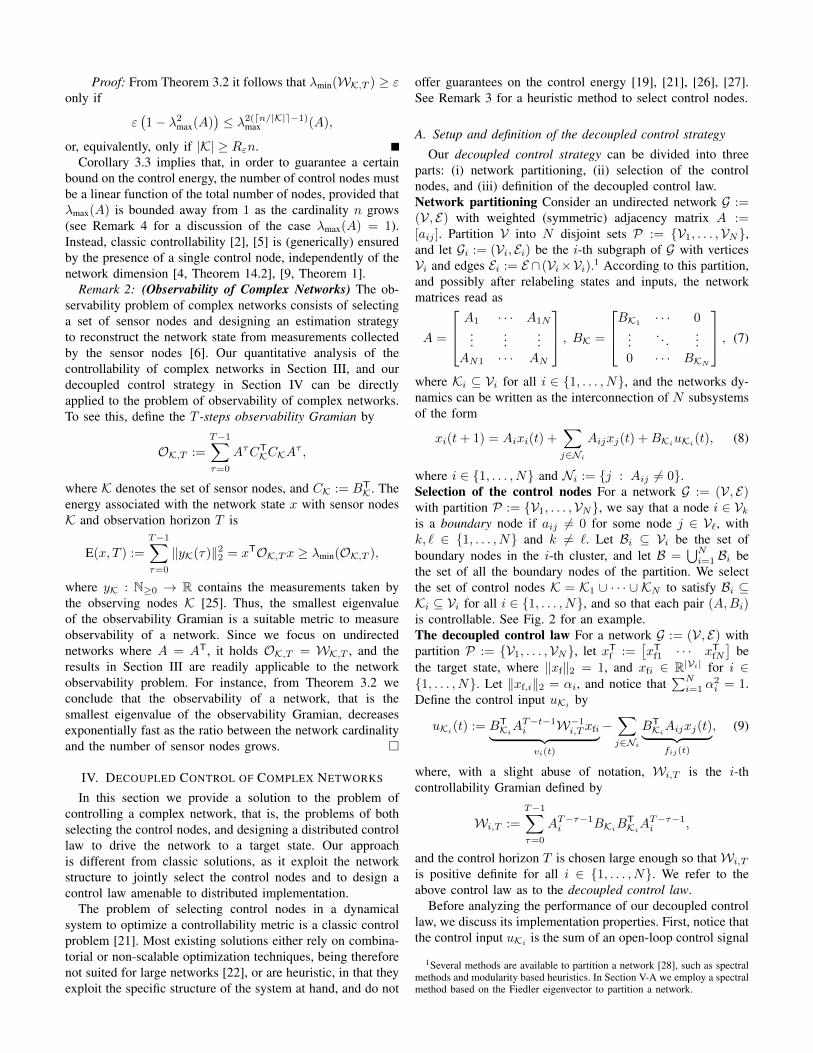
(a) IEEE 118 bus system (b) Klavzar bibliography (c) Pajek network GD99c

Fig. 4. In this figure we report a representation of the example networks in Section V-B. In particular, Fig. 4(a) represents the standard IEEE 118 bus system(118 nodes), Fig. 4(b) represents the Klavzar bibliography network (86 nodes), and Fig. 4(c) represents the GD99c Pajek network (105 nodes). Networksparameters are available at http://www.cise.ufl.edu/research/sparse/matrices/, and their layout is obtained via the graph drawing algorithm described in [36].

0.1 0.2 0.3 0.4 0.5 0.6 0.7 0.8 0.9 1−60

−50

−40

−30

−20

−10

0

10

�min(WK,1)

|K|n

(a) IEEE 118 bus system

0.1 0.2 0.3 0.4 0.5 0.6 0.7 0.8 0.9 1−60

−50

−40

−30

−20

−10

0

10

�min(WK,1)

|K|n

(b) Klavzar bibliography

0.1 0.2 0.3 0.4 0.5 0.6 0.7 0.8 0.9 1−60

−50

−40

−30

−20

−10

0

10

|K|n

�min(WK, n2)

(c) Pajek network GD99c

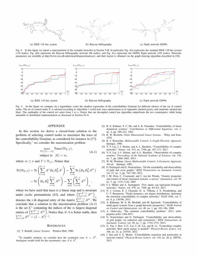
Fig. 5. In this figure we compare (in a logarithmic scale) the smallest eigenvalue of the controllability Gramian for different choices of the set of controlnodes. The set of control nodes K is selected according to Algorithm 1 (solid red), trace optimization as in Appendix (dashed green), and randomly (dashed-dotblue). The cardinality of the control set varies from 1 to n. Notice that our decoupled control law algorithm outperforms the two counterparts, while beingamenable to distributed implementation as discussed in Section IV-A.

APPENDIX

In this section we derive a closed-form solution to theproblem of selecting control nodes to maximize the trace ofthe controllability Gramian, as considered for instance in [17].Specifically,7 we consider the maximization problem

maxK⊆{1,...,n}

Trace(WK,T ),

subject to |K| = m,(A-1)

where m ≤ n and T ∈ N≥1. Notice that

Tr(WK,T ) = Tr

(T−1∑τ=0

AτBKBTKA

τ

)=

T−1∑τ=0

Tr(BKB

TKA

2τ)

= Tr

(BKB

TK

T−1∑τ=0

A2τ

)=∑i∈K

(T−1∑τ=0

A2τ

)ii

,

where we have used that trace is a linear map and is invariantunder cyclic permutations [43], and where

(∑T−1τ=0 A

2τ)ii

denotes the i-th diagonal entry of the matrix∑T−1τ=0 A

2τ . Weconclude that a solution to the maximization problem (A-1)is the set K∗ containing the indices of the m largest diagonalentries of

(∑T−1τ=0 A

2τ)

. Notice that, if A is Schur stable, then∑∞τ=0A

2τ = (I −A2)−1.

REFERENCES

[1] T. Kailath, Linear Systems. Prentice-Hall, 1980.

7To simplify notation, we consider here the symmetric case A = AT.Analogous results hold for the asymmetric case A 6= AT.

[2] R. E. Kalman, Y. C. Ho, and S. K. Narendra, “Controllability of lineardynamical systems,” Contributions to Differential Equations, vol. 1,no. 2, pp. 189–213, 1963.

[3] R. W. Brockett, Finite Dimensional Linear Systems. Wiley and Sons,1970.

[4] K. J. Reinschke, Multivariable Control: A Graph-Theoretic Approach.Springer, 1988.

[5] Y. Y. Liu, J. J. Slotine, and A. L. Barabasi, “Controllability of complexnetworks,” Nature, vol. 473, no. 7346, pp. 167–173, 2011.

[6] Y.-Y. Liu, J.-J. Slotine, and A.-L. Barabasi, “Observability of complexsystems,” Proceedings of the National Academy of Sciences, vol. 110,no. 7, pp. 2460–2465, 2013.

[7] W. M. Wonham, Linear Multivariable Control: A Geometric Approach,3rd ed. Springer, 1985.

[8] G. Parlangeli and G. Notarstefano, “On the reachability and observabilityof path and cycle graphs,” IEEE Transactions on Automatic Control,vol. 57, no. 3, pp. 743–748, 2012.

[9] J. M. Dion, C. Commault, and J. van der Woude, “Generic propertiesand control of linear structured systems: a survey,” Automatica, vol. 39,no. 7, pp. 1125–1144, 2003.

[10] F.-J. Muller and A. Sachuppert, “Few inputs can reprogram biologicalnetworks,” Nature, vol. 478, no. 7369, pp. E4–E4, 2011.

[11] N. J. Cowan, E. J. Chastain, D. A. Vilhena, J. S. Freudenberg, andC. T. Bergstrom, “Nodal dynamics, not degree distributions, determinethe structural controllability of complex networks,” PLOS ONE, vol. 7,no. 6, p. e38398, 2012.

[12] A. Rahmani, M. Ji, M. Mesbahi, and M. Egerstedt, “Controllability ofmulti-agent systems from a graph-theoretic perspective,” SIAM Journalon Control and Optimization, vol. 48, no. 1, pp. 162–186, 2009.

[13] A. Olshevsky, “The minimal controllability problem,” 2013, arXivpreprint arXiv:1304.3071.

[14] G. Notarstefano and G. Parlangeli, “Controllability and observabilityof grid graphs via reduction and symmetries,” IEEE Transactions onAutomatic Control, vol. 58, no. 7, pp. 1719–1731, 2013.

[15] G. Yan, J. Ren, Y.-C. Lai, C.-H. Lai, and B. Li, “Controlling complexnetworks: How much energy is needed?” Physical Review Letters, vol.108, no. 21, p. 218703, 2012.

[16] J. Sun and A. E. Motter, “Controllability transition and nonlocality innetwork control,” Physical Review Letters, vol. 110, no. 20, p. 208701,2013.

[17] T. H. Summers and J. Lygeros, “Optimal sensor and actuator placementin complex dynamical networks,” 2013, arXiv preprint arXiv:1306.2491.

[18] A. C. Antoulas, D. C. Sorensen, and Y. Zhou, “On the decay rate ofHankel singular values and related issues,” Systems & Control Letters,vol. 46, no. 5, pp. 323–342, 2002.

[19] A. M. A. Hamdan and A. H. Nayfeh, “Measures of modal controllabilityand observability for first-and second-order linear systems,” AIAA Jour-nal of Guidance, Control, and Dynamics, vol. 12, no. 3, pp. 421–428,1989.

[20] P. C. Muller and H. I. Weber, “Analysis and optimization of certain qual-ities of controllability and observability for linear dynamical systems,”Automatica, vol. 8, no. 3, pp. 237–246, 1972.

[21] M. Van De Wal and B. De Jager, “A review of methods for input/outputselection,” Automatica, vol. 37, no. 4, pp. 487–510, 2001.

[22] P. L. Sharon and K. K. Rex, “Optimization strategies for sensor andactuator placement,” NASA Langley Technical Report, Tech. Rep., 1999.

[23] B. Marx, D. Koenig, and D. Georges, “Optimal sensor and actuatorlocation for descriptor systems using generalized Gramians and balancedrealizations,” in American Control Conference, Boston, MA, USA, July2004, pp. 2729–2734.

[24] H. R. Shaker and M. Tahavori, “Optimal sensor and actuatorlocation for unstable systems,” Journal of Vibration and Control,2012. [Online]. Available: http://jvc.sagepub.com/cgi/content/abstract/1077546312451302v1

[25] D. Georges, “The use of observability and controllability Gramians orfunctions for optimal sensor and actuator location in finite-dimensionalsystems,” in IEEE Conf. on Decision and Control, New Orleans, LA,USA, Dec. 1995, pp. 3319–3324.

[26] S. S. Rao, T.-S. Pan, and V. B. Venkayya, “Optimal placement ofactuators in actively controlled structures using genetic algorithms,”AIAA Journal, vol. 29, no. 6, pp. 942–943, 1991.

[27] K. B. Lim, “Method for optimal actuator and sensor placement for largeflexible structures,” AIAA Journal of Guidance, Control, and Dynamics,vol. 15, no. 1, pp. 49–57, 1992.

[28] S. Fortunato, “Community detection in graphs,” Physics Reports, vol.486, no. 3-5, pp. 75–174, 2010.

[29] S. Skogestad and I. Postlethwaite, Multivariable Feedback ControlAnalysis and Design, 2nd ed. Wiley, 2005.

[30] W. H. Kwon, Y. S. Moon, and S. C. Ahn, “Bounds in algebraic Riccatiand Lyapunov equations: a survey and some new results,” InternationalJournal of Control, vol. 64, no. 3, pp. 377–389, 1996.

[31] M. E. J. Newman, Networks: An Introduction. Oxford University Press,2010.

[32] M. Fiedler, “Algebraic connectivity of graphs,” Czechoslovak Mathemat-ical Journal, vol. 23, no. 2, pp. 298–305, 1973.

[33] P. Kundur, Power System Stability and Control. McGraw-Hill, 1994.[34] F. Dorfler and F. Bullo, “Synchronization and transient stability in power

networks and non-uniform Kuramoto oscillators,” SIAM Journal onControl and Optimization, vol. 50, no. 3, pp. 1616–1642, 2012.

[35] R. D. Zimmerman, C. E. Murillo-Sanchez, and D. Gan, “MATPOWER:Steady-state operations, planning, and analysis tools for power systemsresearch and education,” IEEE Transactions on Power Systems, vol. 26,no. 1, pp. 12–19, 2011.

[36] Y. Hu, “Efficient, high-quality force-directed graph drawing,” Mathe-matica Journal, vol. 10, no. 1, pp. 37–71, 2005.

[37] M. H. DeGroot, “Reaching a consensus,” Journal of the AmericanStatistical Association, vol. 69, no. 345, pp. 118–121, 1974.

[38] F. Garin and L. Schenato, “A survey on distributed estimation and controlapplications using linear consensus algorithms,” in Networked ControlSystems, ser. LNCIS, A. Bemporad, M. Heemels, and M. Johansson,Eds. Springer, 2010, pp. 75–107.

[39] P. Van Mieghem, J. Omic, and R. Kooij, “Virus spread in networks,”IEEE/ACM Transactions on Networking, vol. 17, no. 1, pp. 1–14, 2009.

[40] V. D. Blondel, J.-L. Guillaume, R. Lambiotte, and E. Lefebvre, “Fastunfolding of communities in large networks,” Journal of StatisticalMechanics: Theory and Experiment, vol. 2008, no. 10, p. P10008, 2008.

[41] J.-C. Delvenne, S. N. Yaliraki, and M. Barahona, “Stability of graphcommunities across time scales,” Proceedings of the National Academyof Sciences, vol. 107, no. 29, pp. 12 755–12 760, 2010.

[42] V. Strassen, “Gaussian elimination is not optimal,” Numerische Mathe-matik, vol. 13, no. 4, pp. 354–356, 1969.

[43] R. A. Horn and C. R. Johnson, Matrix Analysis. Cambridge UniversityPress, 1985.